
Submitted:
14 February 2026
Posted:
28 February 2026
You are already at the latest version
Abstract
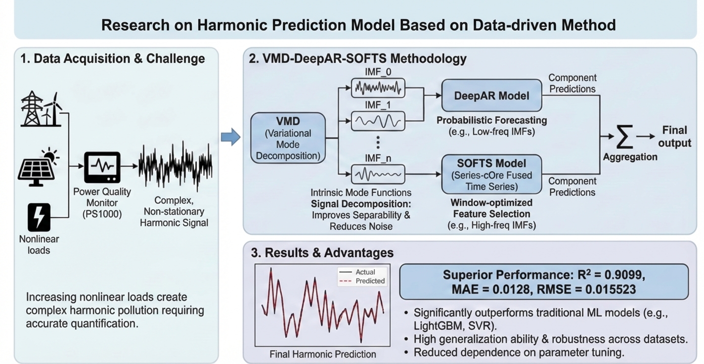
Aiming at the demand of harmonic data quantification and in-depth analysis in power systems, this paper proposes a harmonic data prediction method based on VMD-DeepAR-SOFTS combined model. Firstly, the complex nonlinear and non-stationary harmonic signal was decomposed into multiple Intrinsic mode Functions (IMFs) with different frequency characteristics by using Variational Mode Decomposition (VMD), which effectively improved the separability of the signal and reduced the noise interference. Then, the DeepAR model is used to predict the time series of each IMF component, and the sequential feature selection technology SOFTS based on window optimization is combined to further improve the efficiency of feature extraction and the accuracy of prediction. Experimental results show that the VMD-DeepAR-SOFTS combined model achieves 0.0128, 0.9099 and 0.015523 in MAE, R² and RMSE, respectively, which is significantly better than traditional machine learning models such as LightGBM, XGBoost, CatBoost and SVR. In addition, through the verification of ten groups of independent data sets randomly derived from the system PS1000, the model shows a high degree of consistency and stability, which verifies its excellent generalization ability and robustness. Compared with the single DeepAR or SOFTS model, the combined model has a significant improvement in prediction accuracy and real-time performance. The proposed method not only improves the accuracy of harmonic prediction, reduces the dependence on model parameter tuning, reduces the complexity and cost in practical applications, but also demonstrates its broad application prospects in complex power system environments. Future research will further optimize the model structure, explore more advanced time series decomposition and feature selection techniques to improve the performance of the model, and verify its applicability and effectiveness in more actual power system scenarios.
Keywords:
harmonic data prediction
; variational mode
; decomposition (vMD)
; DeepAR
; SOFTS
; time series forecasting
; power system
1. Introduction
Power quality analysis and power harmonic prediction methods are important topics in power system research. In recent years, with the improvement of modern industrial automation levels, the advancement of new power system construction, and the wide application of new energy systems, power quality issues and harmonic impacts have received increasing attention. The continuous increase in power generation and consumption indicates the rapid development of global industrial automation, information technology, new energy power generation, and other fields. Against this backdrop, more and more devices such as frequency converters, switching power supplies, computer power supplies, inverters, microgrids, and distributed energy systems are connected to the power grid, resulting in a large number of nonlinear and impulse loads in the power system. These loads not only create a simple proportional relationship between current and applied voltage but also generate more nonlinear relationships, thereby producing a large amount of harmonics. These harmonics injected into the power system cause distortion of the originally sinusoidal voltage and current waveforms, forming harmonic pollution and affecting power quality. As modern industrial, commercial, and residential power users' requirements for power quality continue to increase, especially in high-precision manufacturing, data centers, medical facilities, and other fields, harmonic pollution may lead to equipment malfunctions, efficiency reduction, shortened lifespan, and other problems, seriously affecting production efficiency and economic benefits. At the same time, harmonics can cause voltage fluctuations in the power grid, current overload, equipment overheating, insulation aging, and other issues. In severe cases, it can lead to power grid failures, equipment damage, and even large-scale power outages. Therefore, detecting harmonics in the power system is an important means of evaluating power quality performance. Through effective detection and analysis of harmonics, the stable operation of the power system can be ensured, power quality can be improved, and the power demands of users can be met.
Power harmonic detection is a complex process that requires specific methods to separate each harmonic from complex signals and accurately determine the frequency, amplitude, and phase parameters of these harmonics. To conduct harmonic detection and analysis more effectively, many scholars at home and abroad have conducted in-depth research. Currently, many experts have proposed various power harmonic detection methods. Among them, Japanese scholars H. Akagi et al. first proposed the instantaneous reactive power theory in 1984 [1]. Subsequently, many scholars conducted in-depth research based on this theoretical framework and applied it to the field of harmonic detection, proposing the p-q method and ip-iq method that are more suitable for harmonic detection [2]. Both the p-q method and ip-iq method can accurately measure harmonic values in symmetrical three-phase circuits and have good real-time performance. The ip-iq method can accurately detect harmonic currents in asymmetrical three-phase circuits and has a wider range of applications. However, the detection method based on instantaneous reactive power requires the decomposition of three-phase circuits into single-phase circuits when detecting harmonics in single-phase circuits, which is a cumbersome process and requires more electronic components, resulting in higher costs [3]. In addition, the detection results of this method do not include the fundamental wave and only provide the sum of all harmonic components, lacking specific parameter information, which limits its application. Fourier transform has wide applications in signal detection, especially the proposal of the fast Fourier transform (FFT) method has led to the widespread promotion and application of FFT-based power harmonic detection algorithms in practical engineering [4]. However, in actual operation, the continuous-time signal needs to be converted into a finite and discrete signal through sampling technology. This process inevitably introduces A/D conversion errors and may cause the sampling period to be inconsistent with the signal period, resulting in spectral leakage and the fence effect, reducing the accuracy of signal analysis. To alleviate the problem of spectral leakage, scholars and experts from various countries have proposed methods such as approximate synchronous sampling [5], quasi-synchronous sampling [6], and window function methods. Among them, the window function method is widely used due to its ease of implementation and flexible selection of window functions. Common window functions include the Blackman window [7], Hanning window [8], and Kaiser window [9]. To address the fence effect, methods such as the energy center of gravity method [10], phase difference method [11], and interpolation method [12] can be employed. The interpolation method is widely applied due to its high accuracy in error correction. Common interpolation methods include single spectral line interpolation [13], double spectral line interpolation [14], and multi-spectral line interpolation [15]. Subsequent scholars have proposed the combined application of windowing and interpolation [16,17], which significantly improves detection accuracy. However, when analyzing non-stationary harmonics, the FFT algorithm cannot perform localized analysis, resulting in less than ideal detection results. The wavelet transform, with its multi-resolution analysis capability, can perform localized analysis on signals, revealing their characteristics at different scales and frequencies. It is suitable for processing non-stationary and transient signals and shows significant advantages [18]. P.F. Ribeiro [19] was the first to apply the wavelet transform to power harmonic detection, and since then, the wavelet transform and its improved algorithms have been widely used in power harmonic detection, such as the Mallat algorithm [20], discrete wavelet transform [21], wavelet packet transform method [22], and synchrosqueezing wavelet transform [23]. Although the wavelet transform demonstrates significant advantages in processing non-stationary signals and overcomes the shortcomings of the Fourier transform in terms of localization, its signal reconstruction accuracy needs to be improved when detecting stationary harmonics, and it has a frequency aliasing problem, leading to less than ideal detection results, which requires further improvement and refinement [20].
Although existing detection technologies have solved specific problems to a certain extent, each individual technology has inherent limitations and is difficult to fully meet the high-precision detection requirements of harmonics. In the field of power system prediction, many studies focus on improving load prediction accuracy, while there is relatively little research on the prediction of total harmonic distortion (THD). THD is an important factor affecting power quality. Accurate prediction of THD can help identify potential problems in the power system in advance, proactively address harmonic issues, and minimize the impact of harmonics on the power system. Therefore, finding high-precision THD prediction methods is of great importance [24].
Today, harmonic sources in power grids are showing a trend of being massive and complex, especially in distribution networks. Due to the short electrical distances between nodes, there are many harmonic sources that are widely distributed, and the coupling effect between harmonic sources has increased, leading to more significant wideband oscillations [25,26,27]. With the implementation of policies promoting the development of distributed photovoltaics and the large-scale integration of distributed energy, the intermittent, fluctuating, and random nature of the source side has accelerated the changes in the harmonic state of the power grid, making the problem of harmonic over-limitation more severe [28,29]. However, the construction of the power grid harmonic monitoring system is relatively lagging behind, especially in distribution networks and on the user side, where harmonic monitoring has not been scaled up, which limits the analysis and governance of harmonic problems [30,31,32].
Harmonic data mainly come from online power quality monitoring equipment and general measurement methods. Although the online power quality monitoring method can continuously and real-time provide harmonic data, it is costly to cover the entire power grid. The general measurement method is more economical, but the data duration is short and cannot effectively represent the characteristics of harmonics [33,34]. To make up for the insufficiency of harmonic data, scholars have conducted harmonic prediction research through data mining and machine learning techniques. Previous studies have shown that the implementation of harmonic prediction models is similar to load prediction, with methods including those based on association rules [35], chaos theory and least squares support vector machine [36], long short-term memory (LSTM) network models [37,38,39], etc. Relevant research has selected multiple influencing factors as model inputs, such as historical harmonic current [35], power quality data [36,37,38] and environmental factors such as temperature and humidity [39], but there are still difficulties in model parameter tuning and accuracy optimization [36,37,38,39].
In addition, studies have improved existing prediction models, such as the harmonic prediction method combining the Park transformation extraction method and the improved bidirectional LSTM network [40], the prediction method based on the Mind Evolutionary Algorithm (MEA) and the Generalized Regression Neural Network (GRNN) [41], and the research on predicting harmonics in oilfield distribution networks using improved neural network algorithms [42]. Although these methods have achieved good results in terms of accuracy, complexity and the applicability in practical applications remain challenges [41,42].
In harmonic analysis techniques, the Harmonic Balance Method (HBM) has received extensive attention due to its ability to accurately calculate and predict the harmonic characteristics of nonlinear loads, power electronic devices, and distributed energy systems. It has been successfully applied to the modeling and harmonic prediction of microgrids, distributed energy systems, and high-voltage direct current power systems [43,44,45,46]. Meanwhile, studies have also explored harmonic analysis methods based on interpolation Discrete Fourier Transform (DFT) [47], Kalman filtering algorithm [48], S-transform technology [49], and Fast Fourier Transform (FFT) [50], which have shown potential application value in power metering, harmonic suppression, and fault diagnosis [51,52].
Research in the field of new energy has shown that the integration of photovoltaic inverters and wind power generation significantly affects power quality, especially the generation of high-order harmonics and system instability [53,54]. For instance, differences in inverter design significantly affect harmonic levels, while dynamic reactive power compensation technology can effectively improve the power quality of wind power integration [54]. Additionally, the connection of electric vehicle charging stations and electric buses has also brought new harmonic challenges, further highlighting the importance of conducting research on harmonic prediction and control [55]. Despite significant progress in harmonic analysis and prediction methods in theory and experiments, further research is still needed on the harmonic characteristics in actual complex power grids, the impact of dynamic load changes, and the changes in power quality during long-term operation to achieve fault prevention and control through prediction.
In summary, to better quantify harmonic data and conduct in-depth analysis of related harmonics, this paper proposes a harmonic data prediction method based on the DeepAR-SOFTS combined model. The core innovation of this method lies in the combination of the time series prediction model DeepAR in deep learning and the sequence feature selection technology SOFTS based on window optimization. Through this combination, the advantages of both are fully utilized, achieving more accurate and robust harmonic prediction.
Firstly, this paper uses CEEMDAN (Complete Ensemble Empirical Mode Decomposition with Noise Assisted EMD) to decompose the original data, breaking down the complex nonlinear and non-stationary signals into multiple Intrinsic Mode Functions (IMFs) with different frequency characteristics. This decomposition method not only improves the separability of the signal but also effectively reduces the impact of noise on subsequent predictions, ensuring the independence and purity of each IMF component. Secondly, based on the IMF decomposition, this paper predicts the data of different frequencies of IMFs respectively. As an advanced deep learning time series prediction method, the DeepAR model has the ability to handle large-scale, multi-variable data and can capture complex time dependencies and nonlinear patterns. The SOFTS technique further enhances the efficiency and accuracy of feature extraction by optimizing window selection. This divide-and-conquer strategy not only improves the generalization ability of the prediction model but also significantly enhances its adaptability to data volatility. During the prediction stage, the DeepAR-SOFTS combined model makes independent predictions for each IMF component. Finally, by performing cumulative operations on each prediction result, the final harmonic prediction data is obtained. This process ensures the comprehensiveness and accuracy of the prediction results while avoiding the accumulation of biases and errors that may be caused by a single model. Experimental results show that the proposed DeepAR-SOFTS combined model performs excellently in handling the volatility and complexity of harmonic data. Compared with traditional prediction methods, this combined model has significantly improved prediction accuracy and real-time performance. Specifically, the model demonstrates low prediction errors and high robustness in different test scenarios, and can maintain stable prediction performance even when dealing with nonlinear and non-stationary harmonic signals. Additionally, this method effectively addresses the limitations of traditional prediction methods in handling high-frequency harmonics and complex load changes by decomposing and independently predicting each IMF component. The DeepAR-SOFTS combined model not only improves the accuracy of harmonic prediction but also reduces the dependence on model parameter tuning, lowering the complexity and cost in practical applications.
2. Related Methodologies
2.1. DeepAR
DeepAR, proposed by Amazon[58], is a deep learning-based time series forecasting method incorporating a recurrent neural network (RNN). Unlike traditional models, DeepAR takes only the final target value as input and also includes lagged terms such as 1 (previous hour), 1 × 24 (last day), 2 × 24 (two days ago), and 7 × 24 (last week) for hourly data. This approach gives DeepAR an advantage in memory, parameter sharing, and Turing completeness when learning nonlinear features of sequences to enable accurate probability predictions. The DeepAR model is based on the architecture of autoregressive RNNs, utilizing long short-term memory networks (LSTM), and integrating deep learning with probabilistic forecasting to capture long-term dependencies and complex patterns in time series data. Its objective is to estimate the probability distribution of future values in a time series, rather than merely predicting a deterministic point value. Such probabilistic forecasting provides information about the uncertainty of the predictions, thereby aiding in making optimal decisions under uncertainty. Assuming readers have a basic understanding of RNNs and GRUs, this section will briefly introduce the mathematical structure of LSTM before providing detailed explanations of DeepAR's learning and prediction processes.
2.1.1. Long Short-Term Memory
Recurrent Neural Networks (RNN) are a type of neural network that can retain short-term memory, receiving data from both themselves and other neurons. In Long Short-Term Memory (LSTM), a loop employs neurons capable of self-feedback, enabling RNNs to analyze continuous data of varying lengths effectively. LSTM, as a variant of RNN, successfully addresses the challenges associated with gradient explosion or vanishing. The structure of an LSTM unit comprises three essential components: a forget gate (), an input gate (), and an output gate (). Mathematically speaking, LSTM can be represented as follows equation (1):
Among them,,,respectively represent the input, hidden state, and cell state at time. denotes the required stored input candidate with its storage amount regulated by the input gate. represents the internal state at time which is controlled by to discard information selectively; it functions as the output gate.represents the internal state at timewhich is governed byto determine the proportion of information transmitted to the external state.Therefore, can be referred to as 'long-term memory', whilesignifies “short-term memory”. and are weight matrices and serves as a bias vector. activation function is employed for updating the hidden state. The sigmoid function denoted as with formula has a range of values.
2.1.2. Implementation Process of DeepAR
The value of at time step is denoted a.Assuming that in the past, a conditional probability distribution is established for each future time series , as indicated by the likelihood equation (2).
Now, we designate as the reference point for prediction, representing the earliest time point at which the actual unknown value emerges. denotes covariates with known values across all time points in the temporal series. During training, at each time step , the input to the recurrent neural network comprises and the previous time step's state . The learning process of network parameters typically involves the initial computation of the current state, followed by the estimation of likelihood parameters for and ultimately maximizing log-likelihood:
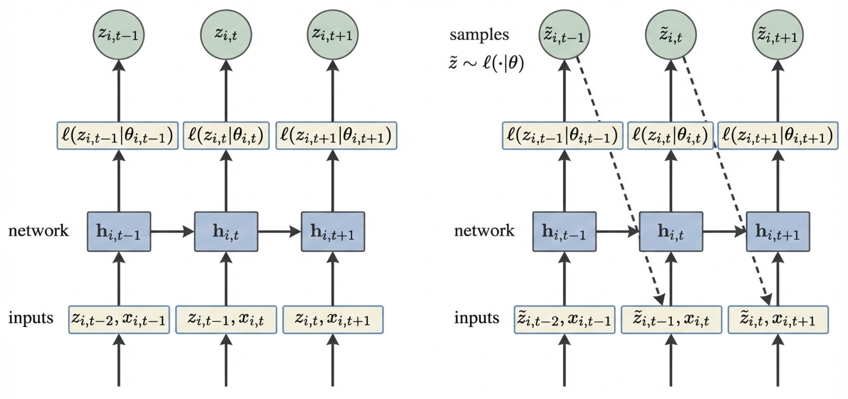
During the training process, a past time interval is selected as the training range, and is chosen for prediction. After completing the training, historical data is input into the network to obtain an initial state . Subsequently, ancestral sampling can be employed to generate predicted results. The values obtained through sampling at each time step within the time interval are denoted as and serves as input for the subsequent time step. By iteratively repeating this process, a series of sampled values from can be acquired. Leveraging these sampled values enables us to compute the desired target value. The specific training and prediction processes of DeepAR are depicted in the diagram below; the left side illustrates the training process and the right side represents the prediction.
Figure 1.
Sumarry of the DeepAR.
The specific expression of is contingent upon the choice of the likelihood function, which in turn needs to be selected based on the statistical characteristics inherent in the data. Commonly employed likelihood models encompass the Gaussian distribution for real-valued data and a negative binomial distribution for non-negative count data (non-negative integers). Other likelihood models such as the beta distribution, Bernoulli distribution, T-distribution, etc., can also be applied here. When employing a Gaussian distribution, it is parameterized using mean and standard deviation: .Herein,is determined by an affine transformation function outputted by the network while is obtained through an affine transformation which follows a softplus activation function to ensure that variance remains more significant than 0. Further details are provided in formula (4):
The affine transformation function employed in this study is the computation of the output generated by the fully connected layer. Assuming, whererepresents an affine transformation followed by a non-linear activation function, the actual calculationinvolves multiplyingwith the weight matrix of that specific layer and subsequently adding an offset term. In essence, the outcome of this affine transformation function serves as input to the ultimate activation function. This article adopts the logarithmic likelihood as its chosen likelihood model.
2.2. SOFTS
SOFTS, the full name of which is Series-cOre Fused Time Series, is an efficient multi-variate time series prediction model based on multi-layer perceptrons (MLPs). This model aims to achieve efficient processing and prediction of time series data through an innovative STar Aggregate-Redistribute (STAR) module. The core of the SOFTS model is a module named STAR, which adopts a centralized strategy to aggregate information from different channels to form a global core representation, and then fuses this core representation with the local representations of each channel to achieve indirect interaction among channels. However, through some designs, the SOFTS model reduces its reliance on the quality of individual channels and enhances its robustness in the face of distribution drift. In terms of computational complexity, compared with traditional attention-based methods, the SOFTS model reduces the computational complexity from quadratic to linear, which is particularly important for processing large-scale datasets. In terms of model universality, the STAR module can not only be used in the SOFTS model but also be integrated as a universal component into other Transformer-based time series prediction models to improve their performance and efficiency.
Implementation Process of SOFTS
The underlying framework of SOFTS is shown in the figure below, and you can see that each sequence is embedded individually and then the embedding is sent to the STAD module. The interactions between each sequence are learned centrally, then assigned to the series and fused together, and finally produced by the linear layer.The specific structure is shown in Figure 2:
Normalization is first used to calibrate the distribution of the input sequence. Normalization of reversible instances is used. It centers the data on the mean of unit variance, and then each series is embedded separately.
Embedding is the process of mapping the original data into a low-dimensional hidden space that captures important features of the data. In the SOFTS model, embeddings help transform the time series data into a form that the model can process more efficiently.
The embedding process is implemented by a linear projection layer, which maps the normalized data to the hidden space, as detailed in Formula (5):
In this way, the embedding contains the information of the whole sequence at all time steps. The embedded series is then sent to the STAD module.
The STAD module is the real difference between the SOFTS model and other prediction methods. A centralized strategy is used to find interactions between all time series.
Firstly, the channel interaction is carried out, and the sequence embedding is refined by multi-layer STAR module. STAR module uses the star structure to exchange information between different channels, as detailed in Formula (6):
The STAR structure is shown in Figure 3:
The embedded sequences are then first passed through the MLP and pooling layer, and this learned representation is then concatenated to form kernels and dispatched to different cliques.
The Core Representation is shown as equation (7):
Here, is the ’th core representation, is a multi-layer perceptron to project the series representation from the series hidden dimension to the core dimension , and is a random pooling operation to aggregate the representations of series.
The Repeat Concatenation part is shown as equation (8):
Here, is the result after concatenating the core representation with each series representation, and the operation copies the core representation C times and concatenates it with each series representation.
The Fusion of series and core is specified in equation (9):
Here, is the series representation at layer and is another multilayer perceptron to fuse the concatenated core and series representations and project them back to the hidden dimension .
Finally, information not captured by the MLP and pooling layers can also be added to the kernel representation via residual connections. Then during the fuse operation, both the kernel representation and its corresponding series of residuals are sent through the MLP layer. The final linear layer uses the output of the STAD module to generate the final prediction for each sequence as shown in Equation (10).
2.3. VMD
VMD (Variational mode decomposition) is an adaptive and completely non-recursive method for modal variation and signal processing. This technique has the advantage of determining the number of mode decomposition, and its adaptability is to determine the number of mode decomposition of the given sequence according to the actual situation, and then adaptively match the optimal center frequency and limited bandwidth of each mode in the process of searching and solving. Moreover, the effective separation of Intrinsic Mode Components (IMFs) and the frequency domain partition of the signal can be achieved, and then the effective decomposition components of the given signal can be obtained, and finally the optimal solution of the variational problem can be obtained.
Implementation Process of VMD
Assuming that the original signal is decomposed into components, the decomposed sequence is guaranteed to be modal components with limited bandwidth with center frequency, and the sum of estimated bandwidths of each mode is minimized. The constraint condition is that the sum of all modes is equal to the original signal, then the VMD constrained variational model is as equation (11).
Here, is the function of each mode and is the center frequency of each mode
By introducing the Lagrange function, the above problem can be transformed into equation:
Here, is the penalty parameter and is the Lagrangian multiplier.
For all , update the functional as equation (13)-(14):
For all:
represents noise. When the signal contains strong noise, can be set to achieve better denoising effect.
The update function is repeated until the following iteration constraints are satisfied as equation(16):
For all the one-sided spectrum of the analytic signal contains only nonnegative frequencies. Finally, the imf obtained by decomposition is obtained.
3. Model Construction
Therefore, this paper proposes a combined multivariate time series prediction model based on VMD-DeepAR-SOFTS after integration. The specific process is as follows: First, the input data is decomposed by VMD, that is, the original data is decomposed into 10 different component signals from low frequency to high frequency. Subsequently, for different component data, DeepAR and SOFTS are used to predict respectively, and the most suitable prediction mode for this component is selected through the program for prediction, and then the prediction components are combined to obtain the final prediction data. The specific process is as Figure 4:
4. Data Selection and Experimental Design
In order to accurately obtain the harmonic component data of the motor current (YVF2-90L-2), the experimental platform was built by using PS1000 power quality field acquisition terminal, frequency converter, motor to be tested and personal computer used for data processing produced by Xuantong Electric Company. The frequency converter is tuned within the allowable frequency range of YVF2-90L-2 motor, and the YVF2-90L-2 motor is kept open for 5 minutes in order to eliminate the influence of potential random factors during the measurement of harmonic data under nominal voltage.
PS1000 power quality field acquisition terminal can quickly detect power quality related parameters, such as harmonic signal, LTHD, frequency, voltage, current and other parameters. And the voltage accuracy of the instrument reaches 0.1%, which is in full compliance with the accuracy requirements of IEC61000-4-31. When the device records data, you can customize the recording duration and capture the maximum, minimum, and average data during this period.
Then, the VMD method mentioned above is adopted to decomposition the original harmonic signal sequence, as shown in Figure 5:
For more accurate prediction, this paper uses the correlation coefficient method in statistics to evaluate the correlation between features and harmonic signals.
Pearson correlation coefficient is an indicator to measure the strong and weak relationship between two groups of data, and its value ranges from [−1,1], in which a result of -1 means completely negative correlation, a result of 0 means no correlation, and a result of 1 means completely positive correlation. The calculation formula is shown in Equation (17):
It can be seen from Figure 6 that PH2, UH2, QH2, UTH2, LTHD2 are relatively strongly correlated with harmonic current. Therefore, these data can be used as the input sequence of the prediction model for model prediction.
4.1. Hardware Parameters
The experiments were implemented using the PyTorch deep learning framework. The computer configuration is as follows: Intel Core i7-8300H processor, NVIDIA GeForce 3060 graphics processor, and 16GB RAM.
4.2. Prediction Model Construction
Based on the above model Settings, this section first uses the DeepAR model and SOFTS to predict the decomposed ten IMF signals (1000 signals in total for each group). Then, the training set, test set and validation set are divided according to the ratio of 8:1:1. Finally, the relevant models are used to predict and verify the data respectively. Then, the program automatically uses the model with better performance to make component prediction, and finally constructs the combined prediction model. Subsequently, another data set collected in the same environment was used for performance verification.
In order to quantify the model performance, the following indicators (equations (18) - (20)) are used to evaluate the model performance:
Where and are the predicted value and the measured value, respectively, and are the average values of the predicted and measured values, respectively.
After testing, the model construction and performance for different components are as Table 1:
Subsequently, the error analysis diagram between the predicted value and the actual value is shown in Figure 7, Figure 7, Figure 8, Figure 9, Figure 10, Figure 11, Figure 12, Figure 13, Figure 14, Figure 15, Figure 16, Figure 17:
To sum up, this paper has completed the construction of the prediction model. That is, DeepAR model is used for IMF0-IMF1 prediction, while SOFTS model is used for IMF2-IMF9 prediction. Finally, all forecast components are summed to obtain the final forecast result. The training results show that DeepAR has excellent fitting effects on IMF0 and IMF1, with R² reaching 0.9026 and 0.8453 respectively. SOFTS performed well on most signals from IMF2 to IMF9, with R-squared values exceeding 0.95, especially IMF9 reaching 0.9942. The combined prediction model is constructed by automatically selecting the optimal model, which further improves the accuracy of the overall prediction.
4.3. Performance Verification and Comparative Test of prediction Model
Subsequently, in order to verify the model performance, the original data are experimentally verified.
At the same time, in order to verify the effectiveness of the model proposed in this paper, LightGBM and other prediction models are selected for comparative experiments, and the specific results are as Table 2:
Based on the experimental results, we evaluate the performance of multiple models in the prediction task. The specific data show that the VMD-DeepAR-SOFTS model performs well in all indicators, with the lowest MAE (0.0128), the highest R² (0.9099) and the lowest RMSE (0.015523), which are significantly better than other traditional machine learning models. For example, the SVR model has a MAE of 0.035736, R² of 0.435446, and RMSE of 0.048092, while the ELM model performs well on MAE (0.032125) and R² (0.517995). However, its RMSE (0.044437) is still higher than that of VMD-DeepAR-SOFTS. In comparison, the MAE of XGBoost and KNN models were 0.044718 and 0.046225, R² was 0.11304 and 0.093730, RMSE was also relatively high, 0.060279 and 0.060932, respectively. It shows low prediction accuracy and explanatory power. The MAE of LightGBM and CatBoost are 0.038265 and 0.038634, R² is 0.363053 and 0.370443, RMSE is 0.051082 and 0.050875, respectively, with medium performance. The MAE of RF, MLP, DT and GBR models ranged from 0.037 to 0.044, R² from 0.184848 to 0.287531, RMSE from 0.050875 to 0.060279. They are inferior to VMD-DeepAR-SOFTS. In particular, although the ELM model is close to VMD-DeepAR-SOFTS in MAE and R², its RMSE is still high. In summary, VMD-DEEPAR-SOFTS model can more effectively capture complex patterns and features in time series data by combining advanced techniques such as VMD (Variational mode decomposition), DeepAR, and SOFTS, thus significantly outperforming other traditional models in prediction accuracy and explanation ability. This shows that the integration of advanced time series decomposition and deep learning methods can significantly improve the overall performance of the model, especially when dealing with complex and variable data.
4.4. Ablation Experiment
In order to verify the effectiveness of the proposed model, this paper uses the original DeepAR and SOFTS to predict the original sequence under the same parameters and experimental environment, and compares the related performance with the combined model. The specific experimental results are as Table 3 and Figure 20 and Figure 21:
Ablation experimental results show that the performance of the combined model is significantly improved compared with the original model after the related strategies. The validity and accuracy of the model proposed in this paper are proved.
4.5. Generalization Experiments
In order to further verify the effectiveness of the selection model, ten groups of data with length 1000 randomly derived from the system are selected for verification experiments, and the performance parameters are obtained as Table 4:
In this validation experiment, the VMD-DeepAR-SOFTS model performs well on ten independently simulated datasets, showing a high degree of consistency and stability. The MAE for all validation sets is maintained between 0.0125 and 0.0132, with an average of about 0.0129, indicating that the model maintains a very low level of error in the forecasting process. The R-squared value fluctuates between 0.9078 and 0.9130, with an average of about 0.9110, showing that the model has excellent explanatory power and can explain about 91.10% of the data variability. Meanwhile, the RMSE is between 0.0153 and 0.0158, with an average of about 0.0155, which further verifies the superior performance of the model in terms of error control. These results show that VMD-DeepAR-SOFTS model not only performs well on a single data set, but also maintains a high level of prediction accuracy and stability on multiple data sets in similar environments, demonstrating its strong generalization ability and robustness. Therefore, this model shows significant advantages in processing complex time series data, and is suitable for prediction tasks requiring high precision and high reliability.
5. Conclusions
In this paper, we propose a new method based on VMD-DeepAR-SOFTS combined model for harmonic data prediction in power systems. By combining Variational Mode Decomposition (VMD), deep learning time series prediction model DeepAR and sequence feature selection technology based on window optimization SOFTS, the proposed method makes full use of their respective advantages to achieve high accuracy and high robustness prediction of complex harmonic data. The main research results of this paper are as follows:
(1) A combined VMD-DEEPAR-SOFTS model is proposed, which effectively integrates the decomposition ability of VMD for nonlinear and non-stationary harmonic signals, the advantages of DeepAR in processing large-scale time series data, and the efficiency of SOFTS in feature selection. Through this multi-level processing strategy, the model can better capture the complex patterns and features in the harmonic data, so as to significantly improve the prediction accuracy and the generalization ability of the model.
(2) Experimental results show that VMD-DeepAR-SOFTS model is significantly superior to traditional machine learning models and single DeepAR or SOFTS model in a variety of evaluation indicators. In multiple test scenarios, the VMD-DeepAR-SOFTS model has the lowest MAE (0.0128), the highest R² (0.9099), and the lowest RMSE (0.015523), showing excellent prediction accuracy and stability. Especially when dealing with nonlinear and non-stationary harmonic signals, the model can still maintain a high prediction performance, which verifies its applicability and reliability in complex power system environment.
(3) The VMD-DeepAR-SOFTS model shows a high degree of consistency and stability through the verification of ten groups of independent data sets randomly derived from the system PS1000. The MAE of all validation sets remains between 0.0125 and 0.0132, the R-squared value remains between 0.9078 and 0.9130, and the RMSE is stable between 0.0153 and 0.0158, which further proves the strong generalization ability and robustness of the model in different data sets and environments.
(4) The VMD-DeepAR-SOFTS model significantly reduces the dependence on model parameter tuning by decomposing and independently predicting each IMF component, and simplifies the operational complexity and cost in practical applications. This feature makes the deployment of the model in real power systems more convenient and efficient.
In summary, the proposed VMD-DeepAR-SOFTS combined model performs well in harmonic data prediction tasks, significantly outperforming existing traditional machine learning methods and single deep learning models. Its high accuracy, stability and good generalization ability make it an ideal choice for dealing with complex power system harmonic prediction tasks. Future research can further optimize the model structure and explore more advanced time series decomposition and feature selection techniques to further improve the performance of the model. In addition, the proposed method can be applied to more real power system scenarios to verify its applicability and effectiveness in different environments and conditions, thus promoting the development of harmonic management and control technology in power systems.
Author Contributions
Conceptualization, Tianxiang Hu and Mingshen Xu; methodology, Tianxiang Hu, Mingshen Xu, and Zihan Bai; software, Tianxiang Hu and Mingshen Xu; validation, Mingshen Xu, Ziyu Zhao, and Zihan Bai; formal analysis, Tianxiang Hu, Mingshen Xu, and Zihan Bai; investigation, Tianxiang Hu, Mingshen Xu, and Ziyu Zhao; resources, Mingshen Xu; data curation, Mingshen Xu; writing—original draft preparation, Tianxiang Hu and Mingshen Xu; writing—review and editing, Mingshen Xu and Ziyu Zhao; visualization, Mingshen Xu; supervision, Mingshen Xu and Ziyu Zhao; project administration, Mingshen Xu and Ziyu Zhao; funding acquisition, Mingshen Xu and Tianxiang Hu. All authors have read and agreed to the published version of the manuscript.
Funding
This work was supported by a research grant (Project Code: B7018425Z011) from the Vocational Training Center of State Grid Jibei Electric Power Company Limited.
Institutional Review Board Statement
Not applicable.
Informed Consent Statement
Not applicable.
Data Availability Statement
The raw data supporting the findings of this study are not publicly available due to privacy and confidentiality restrictions. Access to the data is restricted to protect participant privacy and comply with relevant data protection regulations..
Conflicts of Interest
The authors declare no conflicts of interest.
References
- Akagi, H.; Kanazawa, Y.; Nabae, A. Instantaneous Reactive Power Compensators Comprising Switching Devices without Energy Storage Components. IEEE Transactions on Industry Applications 1984, IA-20, 625-630. [CrossRef]
- Shengqing, L.; Yinghao, Z.; Youqing, Z.; et al. Review of harmonic detection methods in power grid. High Voltage Technology 2004, 39-42.
- Dongxi, P.; day, w.r.s.t. Research status and Development Trend of Harmonic detection in Power System. Electronic Manufacturing 2018, 92-93+95.
- Su, T.; Yang, M.; Jin, T.; Flesch, R.C.C. Power harmonic and interharmonic detection method in renewable power based on Nuttall double-window all-phase FFT algorithm. IET Renewable Power Generation 2018, 12, 953-961. [CrossRef]
- Ferrero, A.; Ottoboni, R. High-accuracy Fourier analysis based on synchronous sampling techniques. IEEE Transactions on Instrumentation and Measurement 1992, 41, 780-785. [CrossRef]
- Dai, X. Quasi-synchronous Sampling and its Application in Non-sinusoidal Power Measurement. Chinese Journal of Scientific Instrument 1984, 55–61.
- Zhou, J.; Wang, X.; Qi, C. Application of interpolated FFT based on Blackman Window Function in Harmonic Signal analysis of Power grid. Journal of Zhejiang University (Science Edition) 2006, 650–653.
- Chen, J.; Wang, W.; Wang, S. Power harmonic FFT analysis Method based on Hanning Self-multiplying window. Power System Protection and Control 2016, 44, 114–121.
- He, Y.; Zhuo, F.; Li, H. Application of Kaiser window in Harmonic current detection. Power Grid Technology 2003, 9–12.
- Chen, P.; Wang, J.; Wu, X. Analysis and Application of Improved FFT Algorithm Based on Energy Center of Gravity Method. Mechanical Science and Technology for Aerospace Engineering 2018, 37, 1883–1889.
- Qi, C.; Chen, L.; Wang, X. Accurate Estimation of harmonic Parameters of Power Grid by interpolating FFT algorithm. Journal of Zhejiang University (Engineering and Technology) 2003, 114–118.
- Bellet, J.-B.; Brachet, M.; Croisille, J.-P. Interpolation on the cubed sphere with spherical harmonics. Numer. Math. 2023, 153, 249-278. [CrossRef]
- Andria, G.; Savino, M.; Trotta, A. Windows and interpolation algorithms to improve electrical measurement accuracy. IEEE Transactions on Instrumentation and Measurement 1989, 38, 856-863. [CrossRef]
- Zhang, H.; Cai, X.; Lu, G.-F. Harmonic analysis of power based on improved bispectral interpolation FFT algorithm. Hydropower Energy Science 2014, 32, 185–188.
- Chen, Z.; Wang, L.; Wang, C. Power harmonic analysis Method based on Combined Cosine Optimization Window four-line interpolation FFT. Power Grid Technology 2020, 44, 1105–1113.
- Su, X.; Zhang, H.; Chen, L.; Qin, L.; Yu, L. Improved Parameter Identification Method for Envelope Current Signals Based on Windowed Interpolation FFT and DE Algorithm. Algorithms 2018, 11, 113. [CrossRef]
- Qian, H.; Zhao, R.; Chen, T. Interharmonics Analysis Based on Interpolating Windowed FFT Algorithm. IEEE Transactions on Power Delivery 2007, 22, 1064-1069. [CrossRef]
- Galli, A.W.; Heydt, G.T.; Ribeiro, P.F. Exploring the power of wavelet analysis. IEEE Comput. Appl. Power 1996, 9, 37-41. [CrossRef]
- Shao, M.; Zhong, Y.-R.; Yu, J.-M. Real-time detection method of Harmonic current based on Wavelet transform. Power Electronics Technology 2000, 42–45.
- Zhang, P.; Li, H. A method for harmonic Analysis based on discrete wavelet Transform. Transactions of China Electrotechnical Society 2012, 27, 252–259.
- Yin, X. Application of Wavelet packet Transform in Harmonic Detection of Power Grid. Journal of Huaiyin Normal University (Natural Science Edition) 2002, 43–46.
- Wang, X.; Li, C.; Yan, X. Nonstationary harmonic signal extraction from strong chaotic interference based on synchrosqueezed wavelet transform. Signal, Image and Video Processing 2018, 13, 397 - 403.
- Yuan, D.; Liu, Y.; Lan, M.; Jin, T.; Mohamed, M.A. A Novel Recognition Method for Complex Power Quality Disturbances Based on Visualization Trajectory Circle and Machine Vision. IEEE Transactions on Instrumentation and Measurement 2022, 71, 1-13. [CrossRef]
- Wang, Y. Review of research development in power quality disturbance detection. Power System Protection and Control 2021, 49, 174–186.
- Wang, X.; Blaabjerg, F. Harmonic Stability in Power Electronic-Based Power Systems: Concept, Modeling, and Analysis. IEEE Transactions on Smart Grid 2019, 10, 2858-2870. [CrossRef]
- Iturrino-García, C.; Patrizi, G.; Bartolini, A.; Ciani, L.; Paolucci, L.; Luchetta, A.; Grasso, F. An Innovative Single Shot Power Quality Disturbance Detector Algorithm. IEEE Transactions on Instrumentation and Measurement 2022, 71, 1-10. [CrossRef]
- Cui, C.; Duan, Y.; Hu, H.; Wang, L.; Liu, Q. Detection and Classification of Multiple Power Quality Disturbances Using Stockwell Transform and Deep Learning. IEEE Transactions on Instrumentation and Measurement 2022, 71, 1-12. [CrossRef]
- Yu, B.; Hu, L.; Wang, J. Study on harmonic current prediction method based on sequence data analysis. Power Capacitor & Reactive Power Compensation 2016, 37, 66-70.
- Lin, S.; Tang, J.; Tang, B. Study on forecasting model of typical power quality steady-state indices. Power System Technology 2018, 42, 624–630.
- Liu, Q.; Yin, W.; Hu, W. Prediction of power harmonic monitoring data based on LSTM algorithm. Power Capacitor & Reactive Power Compensation 2019, 40, 139–145.
- Zhang, H.; Li, Y.; Wang, Q.; et al. Online evaluation of measurement accuracy of power quality monitoring devices based on LSTM. China Measurement & Test 2022, 48, 253-259.
- Yang, P.; Wang, X.; Zhao, X. Research on harmonic prediction of the grid-connected photovoltaic system based on deep learning. Advances of Power System & Hydroelectric Engineering 2022, 38, 71–80.
- Yang, J.; Ma, H.; Dou, J.; Guo, R. Harmonic Characteristics Data-Driven THD Prediction Method for LEDs Using MEA-GRNN and Improved-AdaBoost Algorithm. IEEE Access 2021, 9, 31297-31308. [CrossRef]
- Yang, X. The application of BP neural network in the ship power grid harmonic prediction. Ship Science and Technology 2016, 38, 55–57.
- Diahovchenko, I.; Volokhin, V.; Kurochkina, V.; Špes, M.; Kosterec, M. Effect of harmonic distortion on electric energy meters of different metrological principles. Front. Energy 2019, 13, 377-385. [CrossRef]
- Acharya, S.; Ghosh, R.; Halder, T. An adverse effect of the harmonics for the power quality issues. In Proceedings of the 2016 International Conference on Computational Techniques in Information and Communication Technologies (ICCTICT), 11-13 March 2016, 2016; pp. 569-574.
- Silva, R.P.B.d.; Quadros, R.; Shaker, H.R.; Silva, L.C.P.d. Harmonic Interaction Effects on Power Quality and Electrical Energy Measurement System. In Proceedings of the 2019 International Symposium on Advanced Electrical and Communication Technologies (ISAECT), 27-29 Nov. 2019, 2019; pp. 1-7.
- Lu, J.; Zhao, X.; Hui, L. Harmonic analysis in Microgrid and distributed energy system using Harmonic Balance Method. In Proceedings of the 2016 IEEE PES Asia-Pacific Power and Energy Engineering Conference (APPEEC), 25-28 Oct. 2016, 2016; pp. 262-266.
- Zhao, X.; Lu, J.; Seagir, A. Harmonic Balance Method and Its Application in Electrical Power and Renewable Energy Systems. In Proceedings of the 2021 IEEE PES Innovative Smart Grid Technologies - Asia (ISGT Asia), 5-8 Dec. 2021, 2021; pp. 1-5.
- Lu, J.; Taghizadeh, S.; Hossain, M.J.; Zhao, X. Harmonic balance method used for harmonics calculation and prediction in power systems. In Proceedings of the 2016 Australasian Universities Power Engineering Conference (AUPEC), 25-28 Sept. 2016, 2016; pp. 1-6.
- Lu, J. Harmonic Balance Methods used in Power Electronics and Distributed Energy System. In Proceedings of the 2018 IEEE International Power Electronics and Application Conference and Exposition (PEAC), 4-7 Nov. 2018, 2018; pp. 1-6.
- Bogusz, P.; Korkosz, M.; Prokop, J. Current harmonics analysis as a method of electrical faults diagnostic in switched reluctance motors. In Proceedings of the 2007 IEEE International Symposium on Diagnostics for Electric Machines, Power Electronics and Drives, 6-8 Sept. 2007, 2007; pp. 426-431.
- Zhao, G.; Yue, Y. Harmonic analysis and suppression of electric vehicle charging station; 2017; pp. 347-351.
- Leou, R.C.; Teng, J.H.; Su, C.L. Power Quality Analysis of Electric Transportation on Distribution Systems. In Proceedings of the 2016 3rd International Conference on Green Technology and Sustainable Development (GTSD), 24-25 Nov. 2016, 2016; pp. 28-33.
- Mostafa, M.A. Kalman Filtering Algorithm for Electric Power Quality Analysis: Harmonics and Voltage Sags Problems. In Proceedings of the 2007 Large Engineering Systems Conference on Power Engineering, 10-12 Oct. 2007, 2007; pp. 159-165.
- Rustemli, S.; Satici, M.A.; Şahin, G.; van Sark, W. Investigation of harmonics analysis power system due to non-linear loads on the electrical energy quality results. Energy Reports 2023, 10, 4704-4732. [CrossRef]
- Jaipradidtham, C. A control of real voltage and harmonic analysis with adaptive static var of electric arc furnace for power quality improvement by Grey Markov method. In Proceedings of the 2016 IEEE 6th International Conference on Power Systems (ICPS), 4-6 March 2016, 2016; pp. 1-6.
- Zhang, W.; Ling, B. Harmonic Detection Method of Electric Equipment Malfunction; 2018; pp. 375-382.
- Jiao, L.; Du, Y. An approach for electrical harmonic analysis based on interpolation DFT. Archives of Electrical Engineering 2022, 71, 445-454. [CrossRef]
- Luo, z.; Xu, z.; Zheng, y.; Lu, x. DFT and DSP-based electric energy measurement algorithm of harmonic source load. In Proceedings of the Proceedings. International Conference on Power System Technology, 13-17 Oct. 2002, 2002; pp. 2487-2490 vol.2484.
- Chen, M.; Roberts, C.; Weston, P.; Hillmansen, S.; Zhao, N.; Han, X. Harmonic modelling and prediction of high speed electric train based on non-parametric confidence interval estimation method. International Journal of Electrical Power & Energy Systems 2017, 87, 176-186. [CrossRef]
- Wu, T.; Jiang, D.; Wang, Y.; Lei, A. Study on a Harmonic Measurement and Analysis Method for Power Supply System. Int. J. Emerging Electr. Power Syst. 2017, 18. [CrossRef]
- Solowiej, P.; Lange, A.; Neugebauer, M.; Dach, J. The quality of electricity generated by inverters in photovoltaic systems. In Proceedings of the Proceedings of the 3rd International Conference on Energy and Environment (ICEE), 2017, 2017.
- Othman, A. Harmonic distortion effect on operation of power systems. In Proceedings of the Proceedings of the 6th International Power Engineering Conference, 2006, 2006.
- Ali, M. Harmonics in modern power system due to power electronic devices and their effects. In Proceedings of the International Conference on Power Systems, Energy, Environment (ICPEE), 2016.
Figure 2.
Summary of the SOFTS.
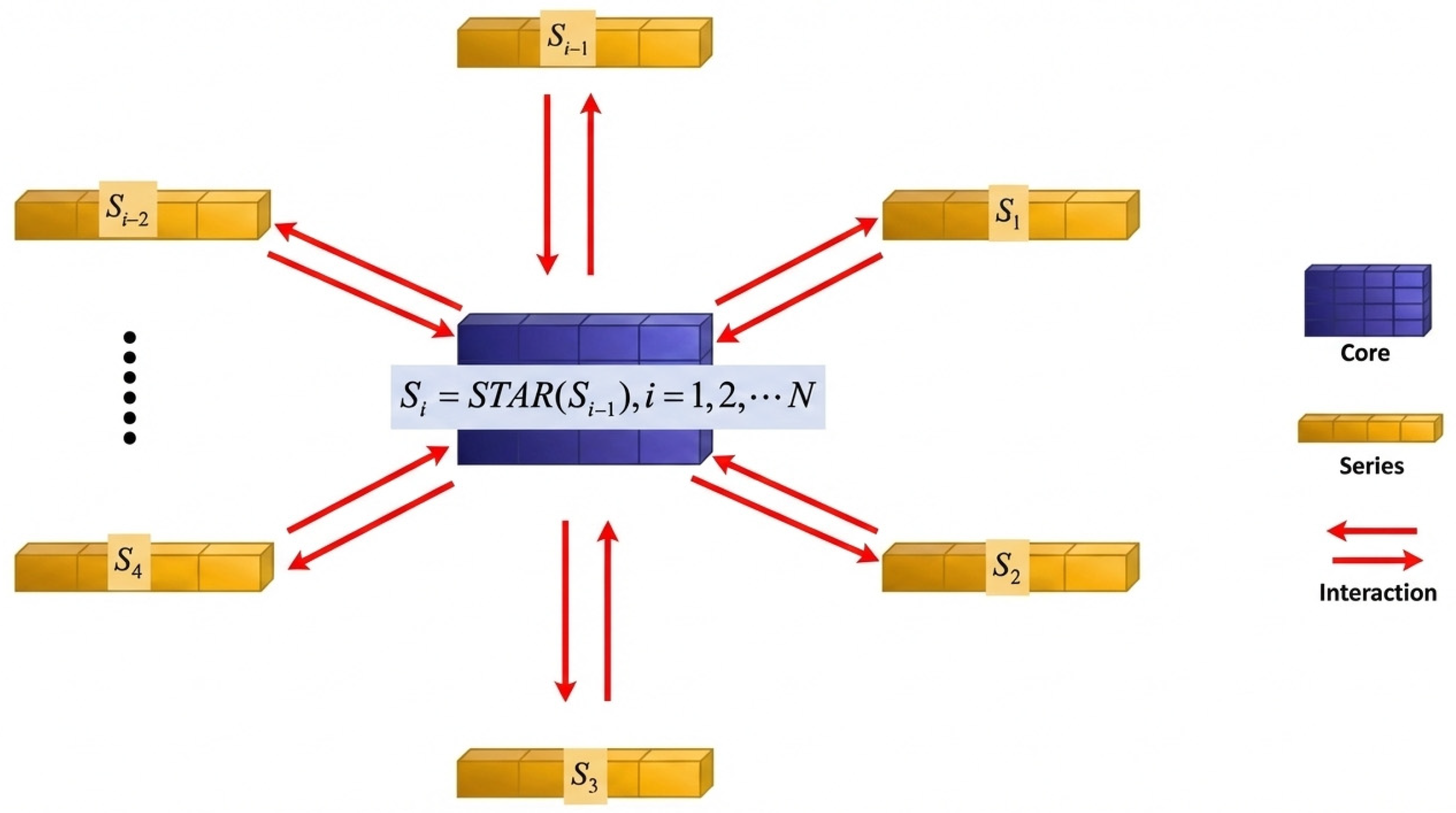
Figure 3.
Process of the contralized interaction star.
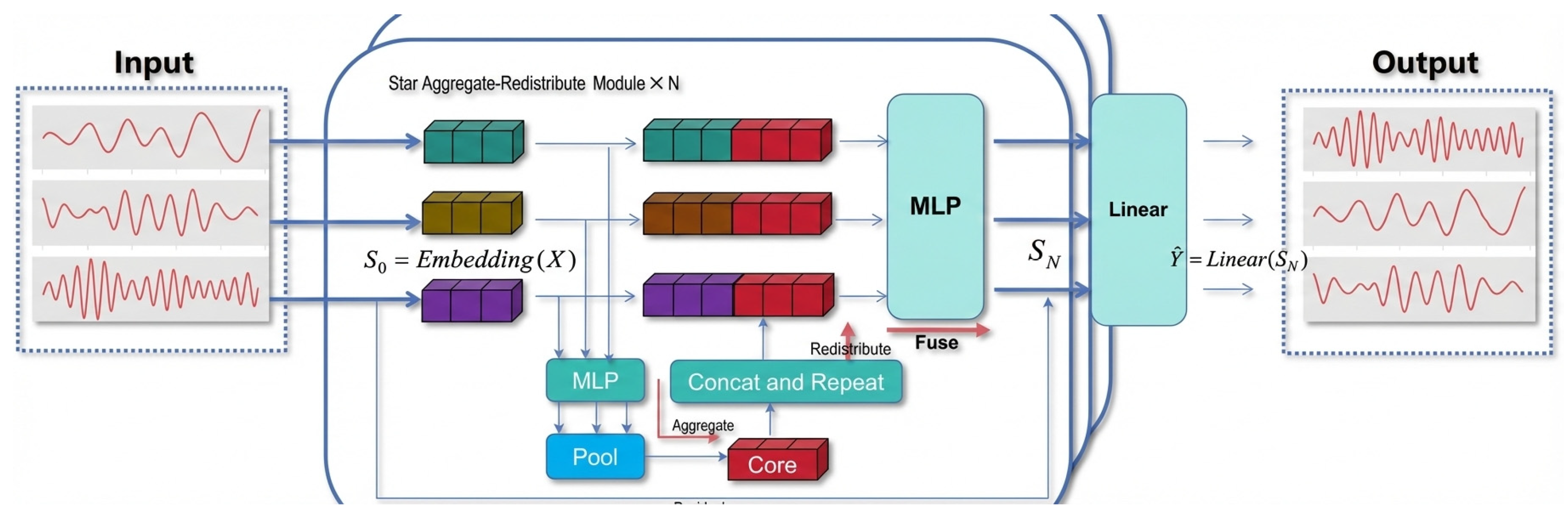
Figure 4.
Summary of our model.
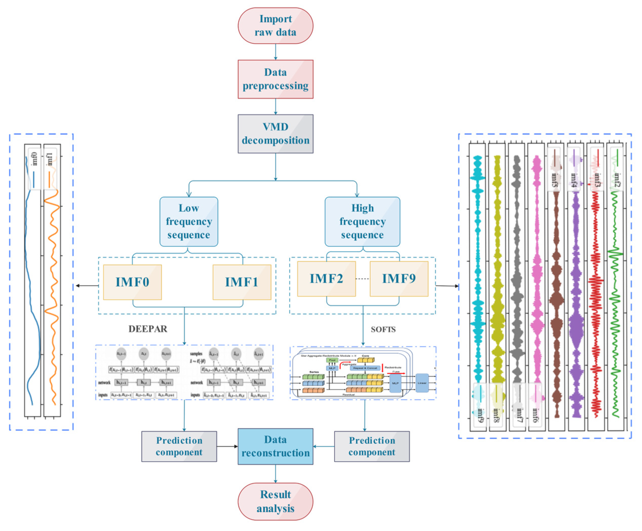
Figure 5.
Schematic diagram of VMD decomposition.
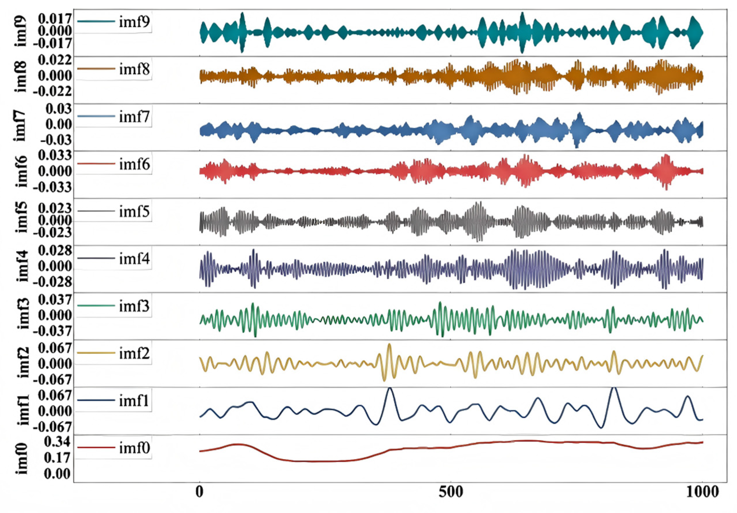
Figure 6.
Correlation matrix heat map.
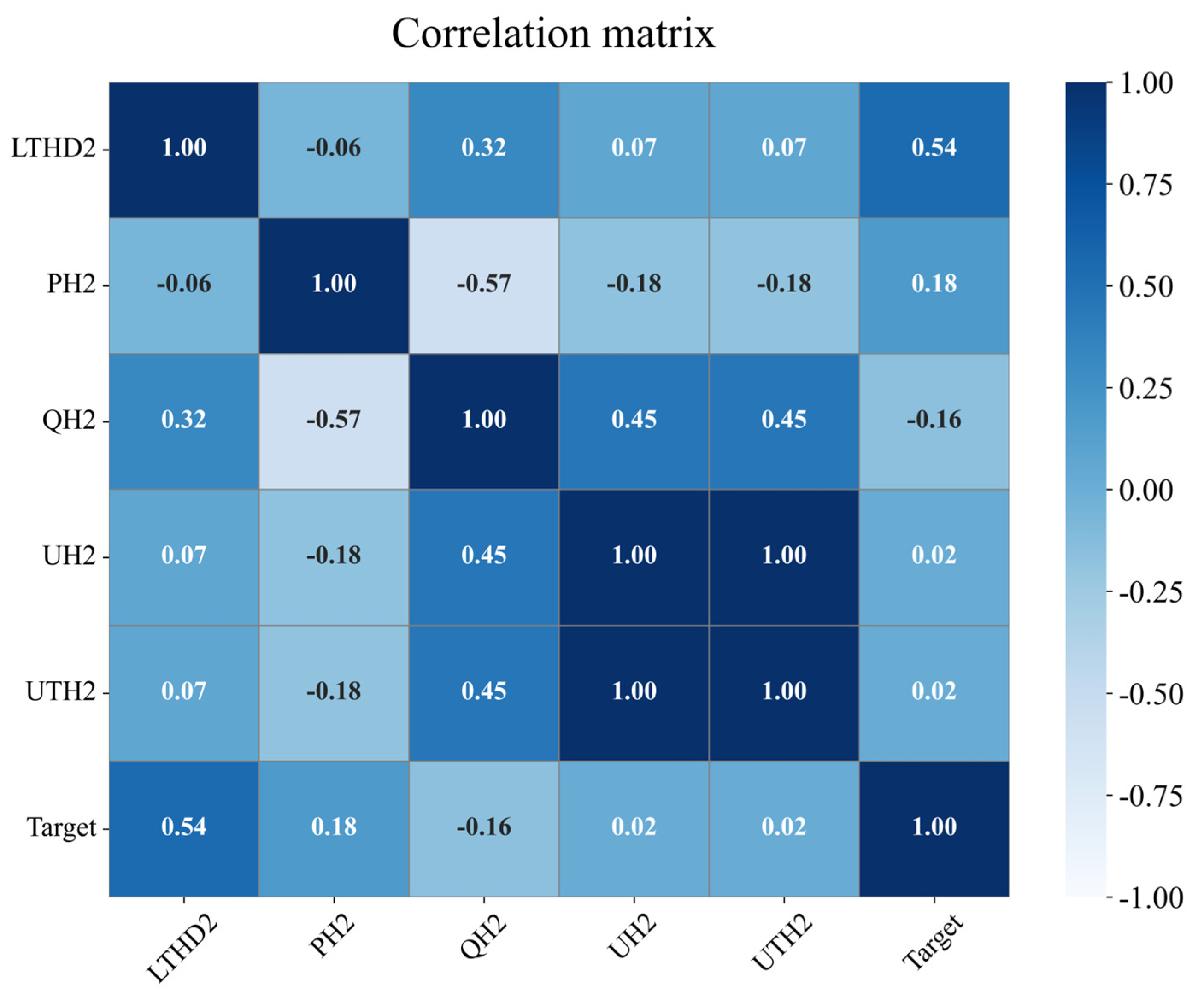
Figure 7.
IMF0 prediction error visualization. (a) Percentage error visualization; (b) Prediction scatter plot analysis.
Figure 7.
IMF0 prediction error visualization. (a) Percentage error visualization; (b) Prediction scatter plot analysis.
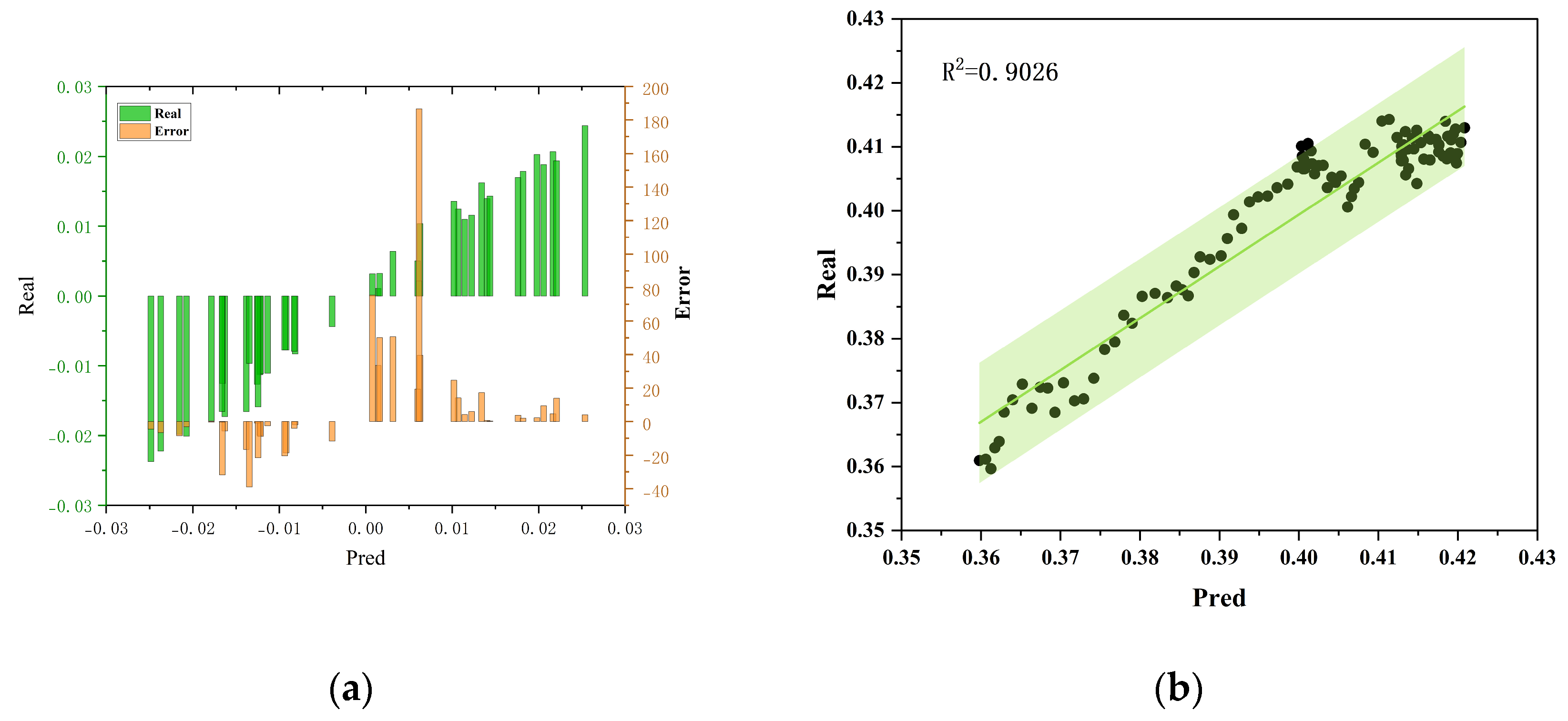
Figure 8.
IMF1 prediction error visualization. (a) Percentage error visualization; (b) Prediction scatter plot analysis.
Figure 8.
IMF1 prediction error visualization. (a) Percentage error visualization; (b) Prediction scatter plot analysis.
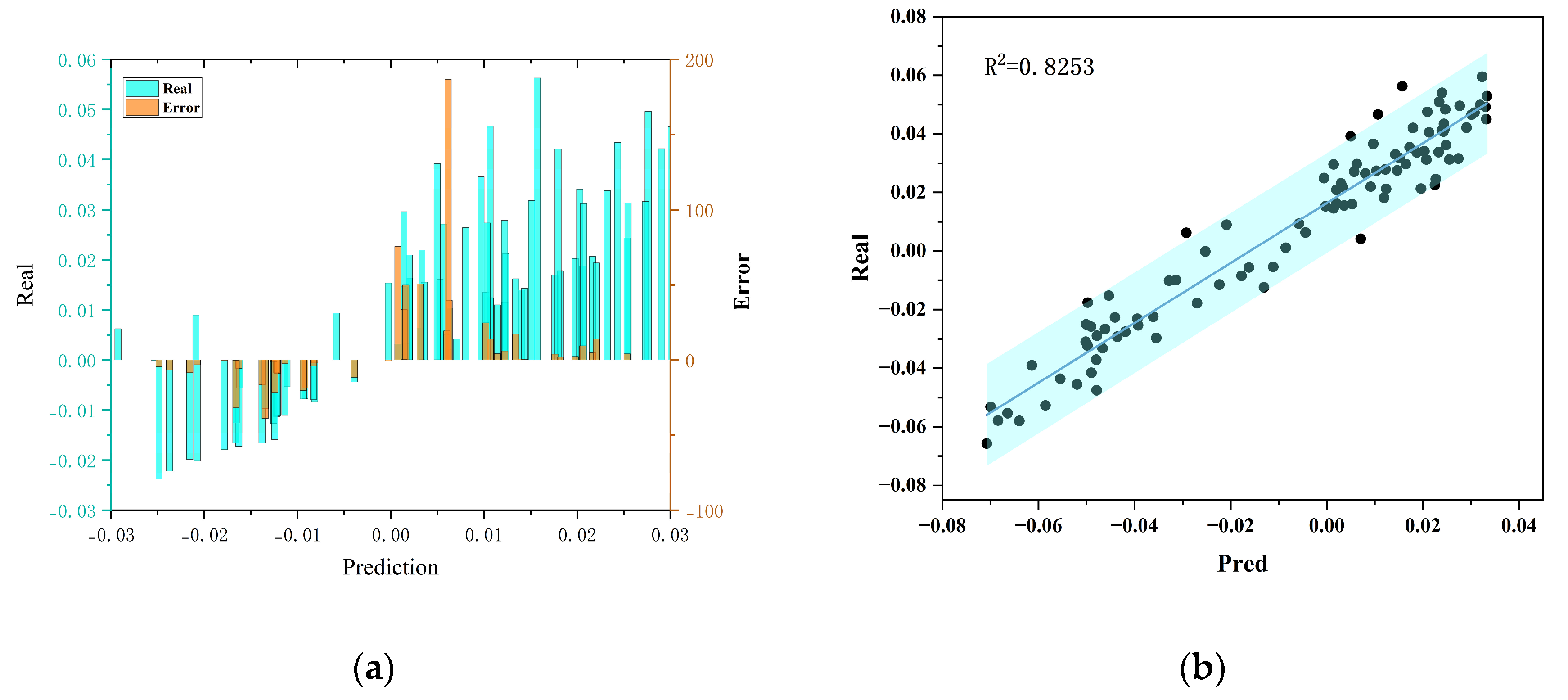
Figure 9.
IMF2 prediction error visualization. (a) Percentage error visualization; (b) Prediction scatter plot analysis.
Figure 9.
IMF2 prediction error visualization. (a) Percentage error visualization; (b) Prediction scatter plot analysis.
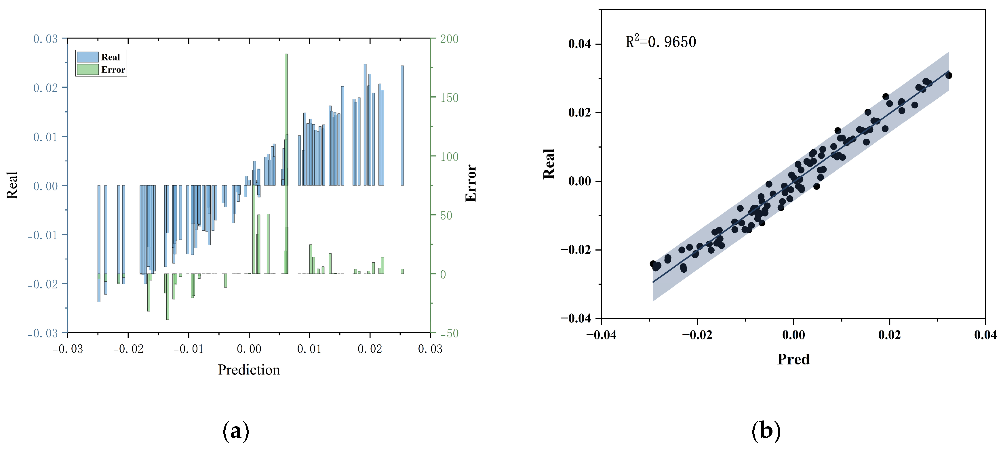
Figure 10.
IMF3 prediction error visualization. (a) Percentage error visualization; (b) Prediction scatter plot analysis.
Figure 10.
IMF3 prediction error visualization. (a) Percentage error visualization; (b) Prediction scatter plot analysis.
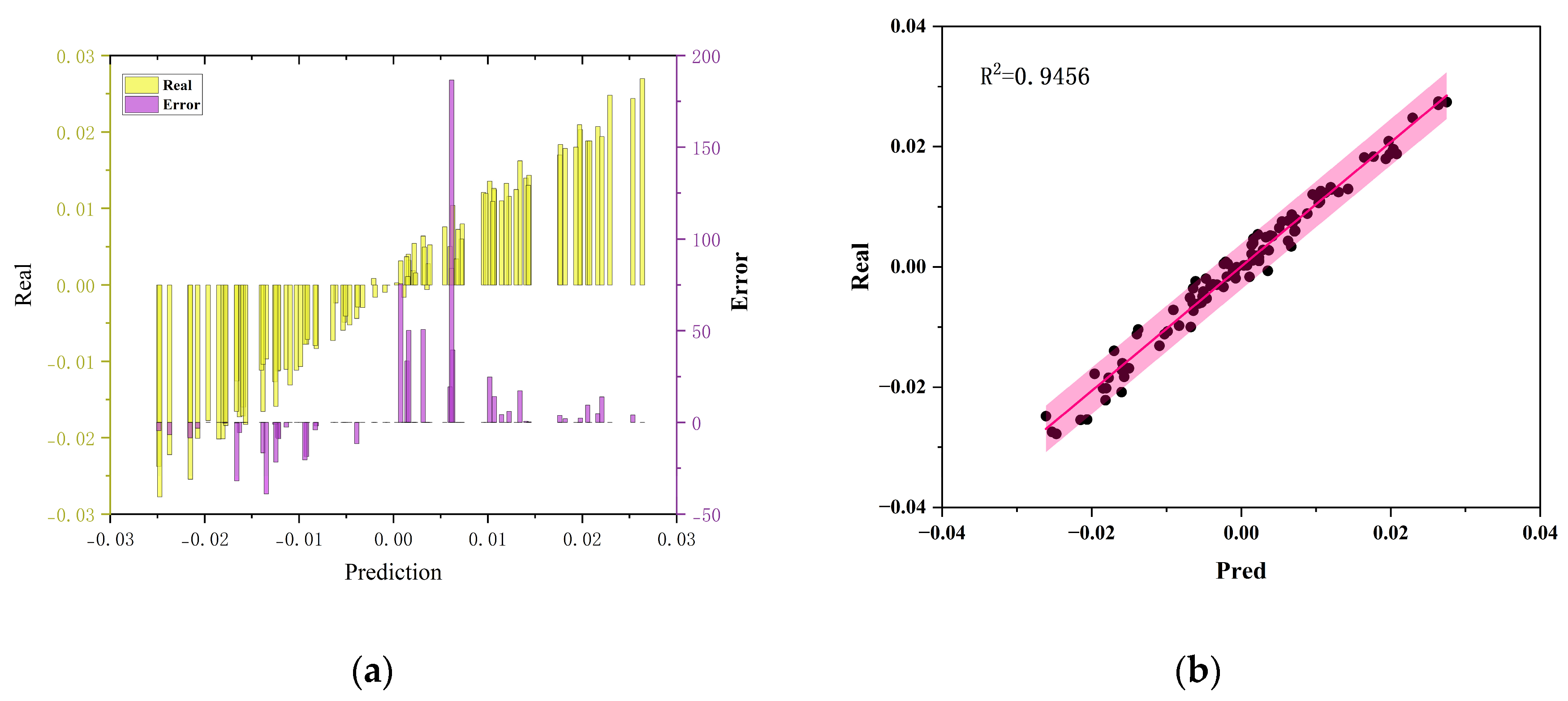
Figure 11.
IMF4 prediction error visualization. (a) Percentage error visualization; (b) Prediction scatter plot analysis.
Figure 11.
IMF4 prediction error visualization. (a) Percentage error visualization; (b) Prediction scatter plot analysis.
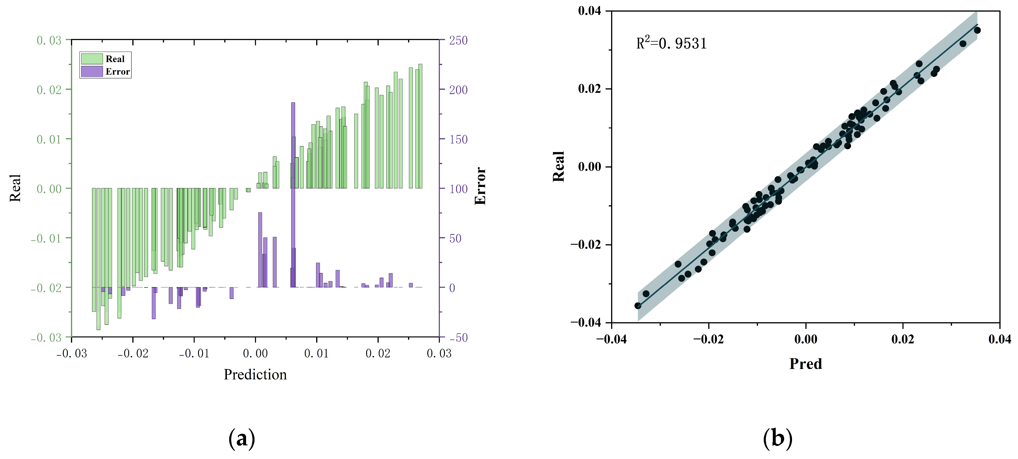
Figure 12.
IMF5 prediction error visualization. (a) Percentage error visualization; (b) Prediction scatter plot analysis.
Figure 12.
IMF5 prediction error visualization. (a) Percentage error visualization; (b) Prediction scatter plot analysis.
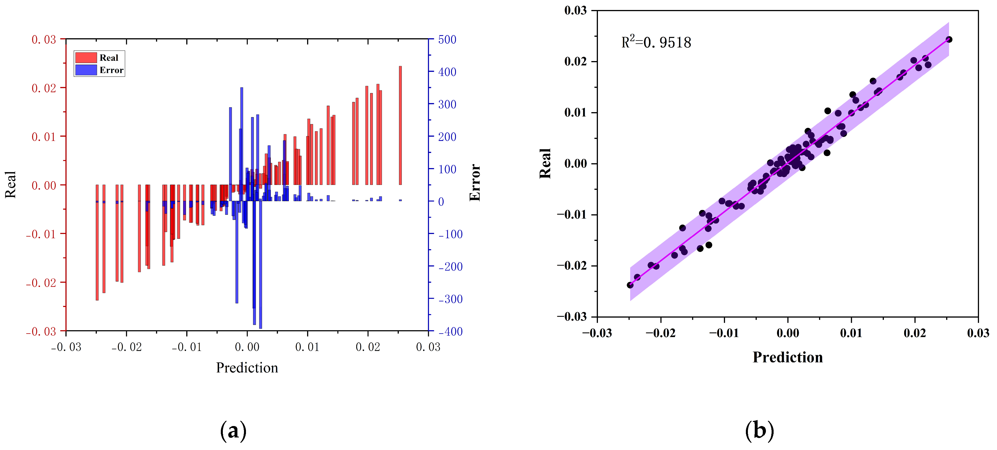
Figure 13.
IMF6 prediction error visualization. (a) Percentage error visualization; (b) Prediction scatter plot analysis.
Figure 13.
IMF6 prediction error visualization. (a) Percentage error visualization; (b) Prediction scatter plot analysis.
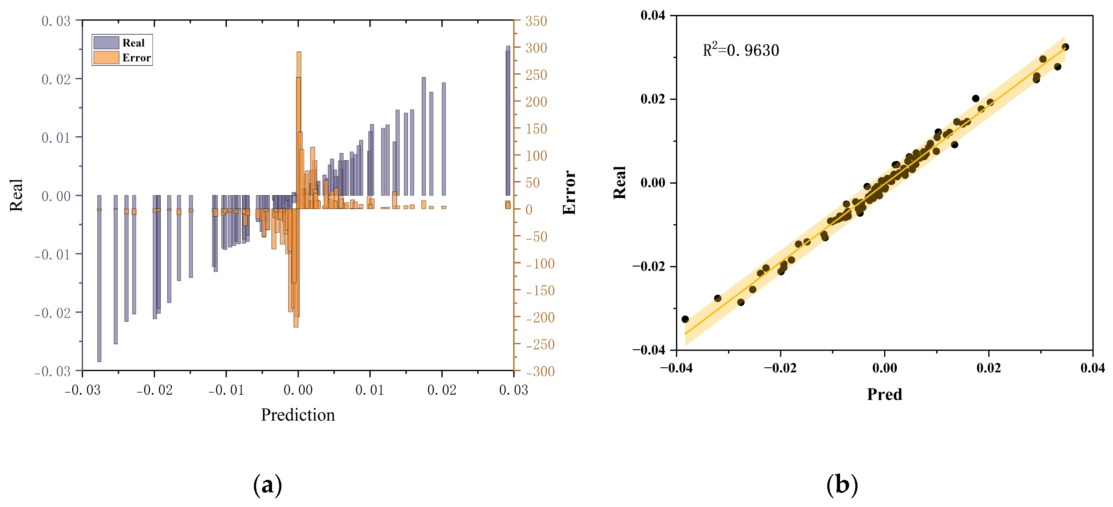
Figure 14.
IMF7 prediction error visualization. (a) Percentage error visualization; (b) Prediction scatter plot analysis.
Figure 14.
IMF7 prediction error visualization. (a) Percentage error visualization; (b) Prediction scatter plot analysis.
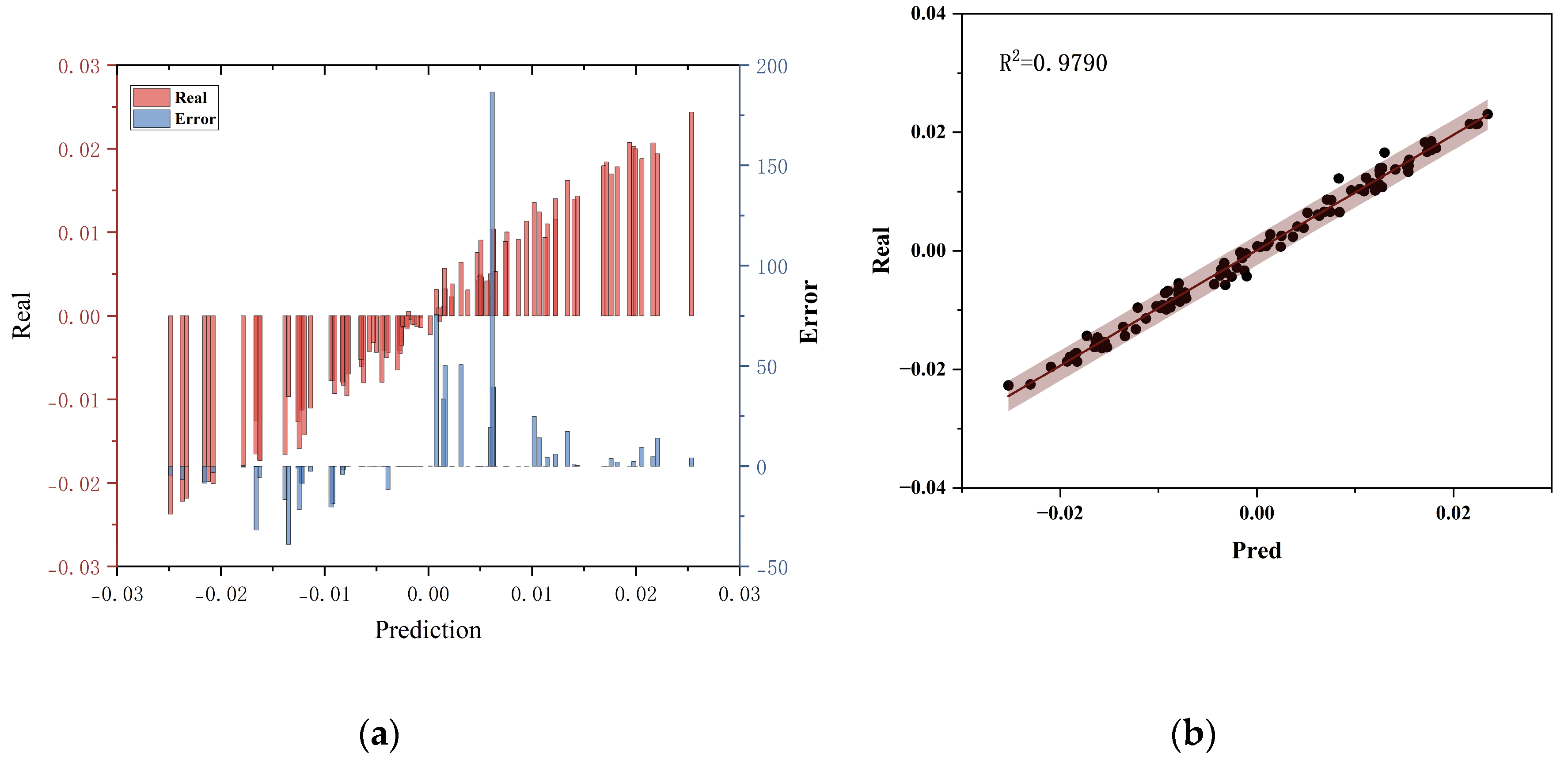
Figure 15.
IMF8 prediction error visualization. (a) Percentage error visualization; (b) Prediction scatter plot analysis.
Figure 15.
IMF8 prediction error visualization. (a) Percentage error visualization; (b) Prediction scatter plot analysis.
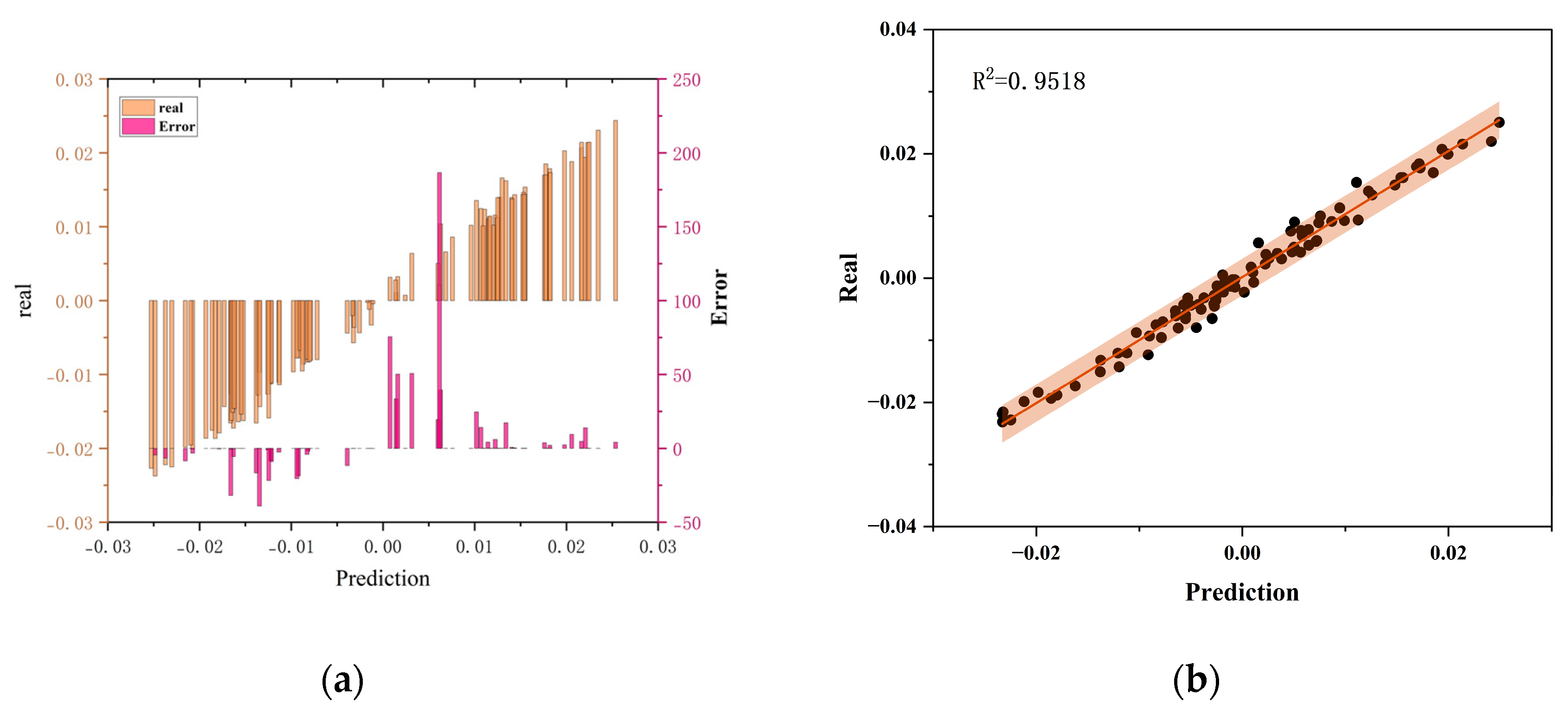
Figure 16.
IMF9 prediction error visualization. (a) Percentage error visualization; (b) Prediction scatter plot analysis.
Figure 16.
IMF9 prediction error visualization. (a) Percentage error visualization; (b) Prediction scatter plot analysis.
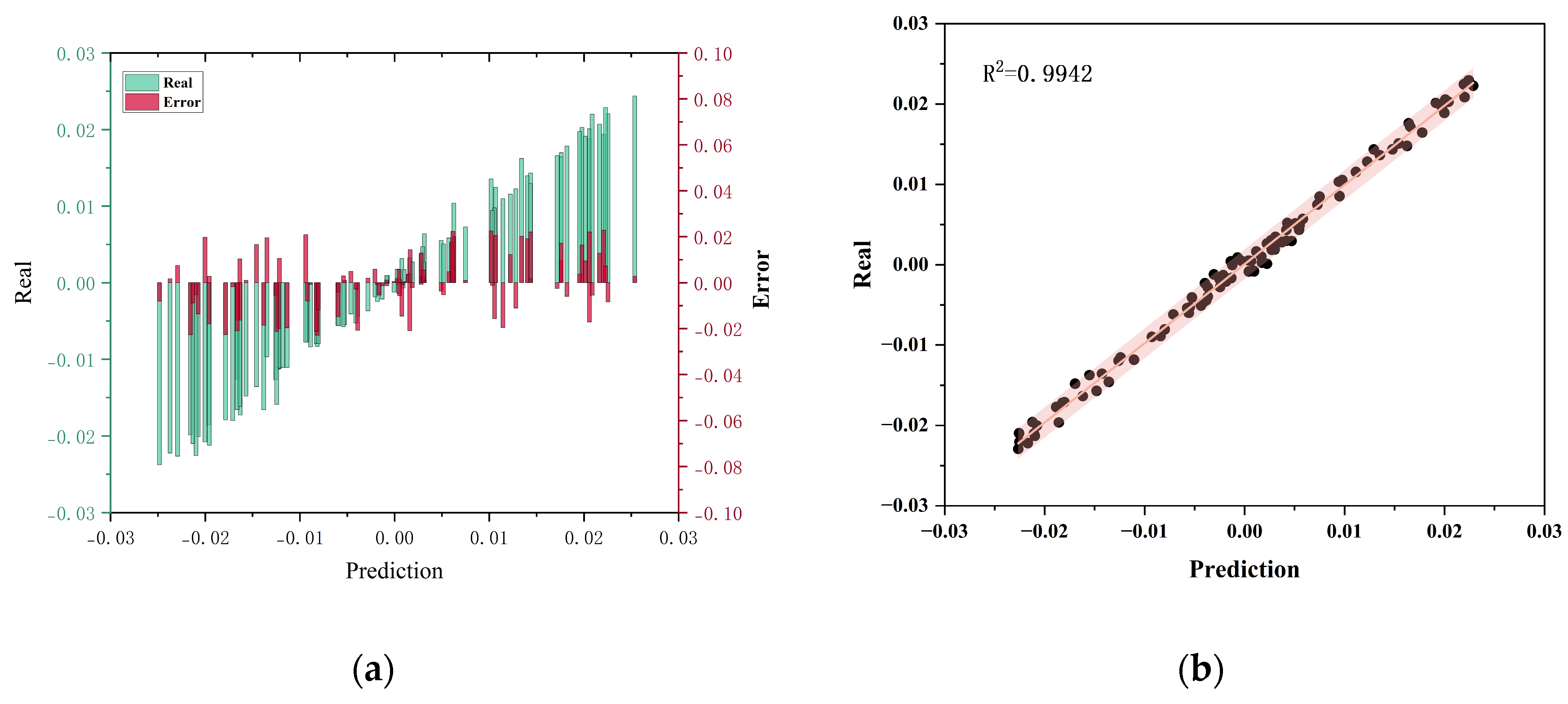
Figure 17.
Comparison of TID Predictions by Various Models.
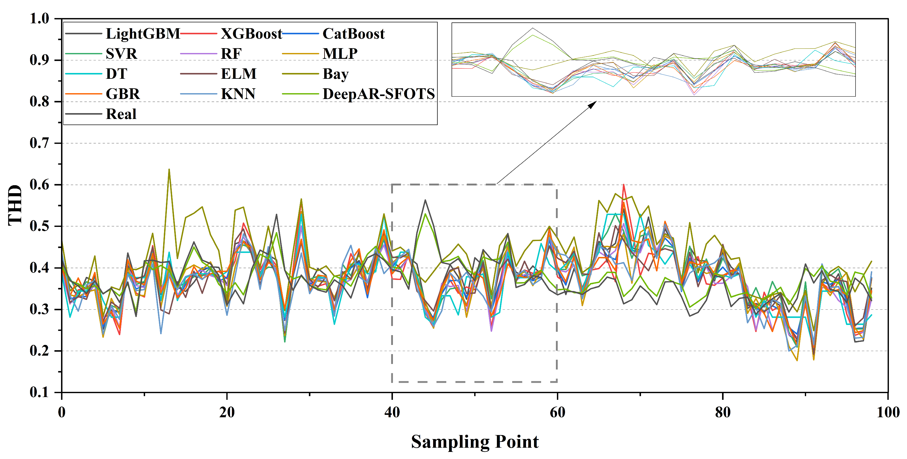
Figure 18.
Error visualization of each prediction algorithm.
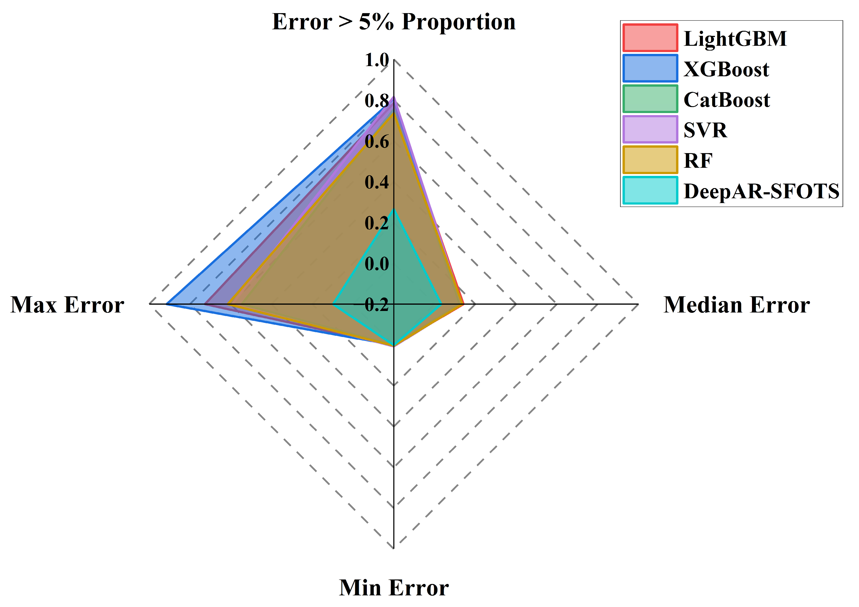
Figure 19.
Error visualization of each prediction algorithm.
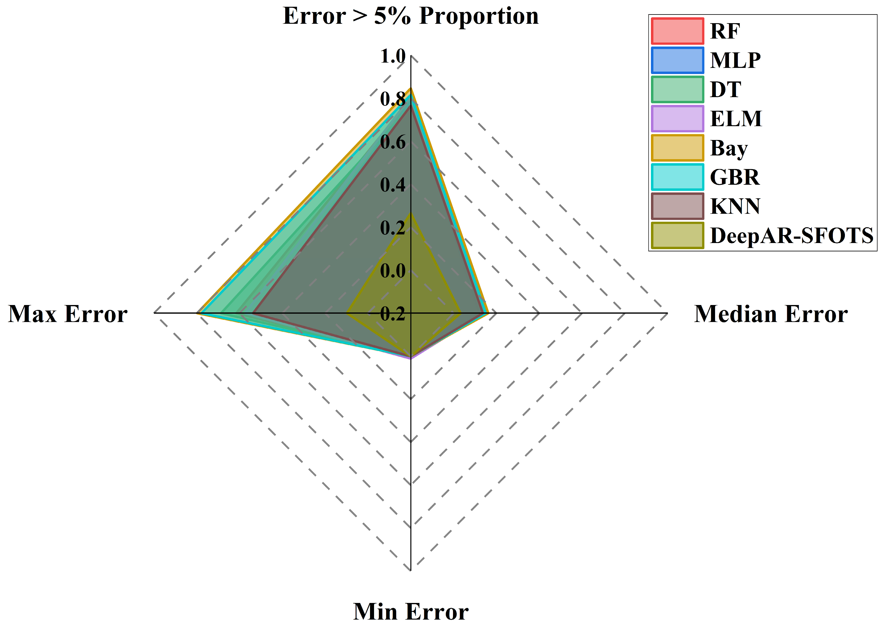
Figure 20.
Comparison of the prediction of TID by ablation models.
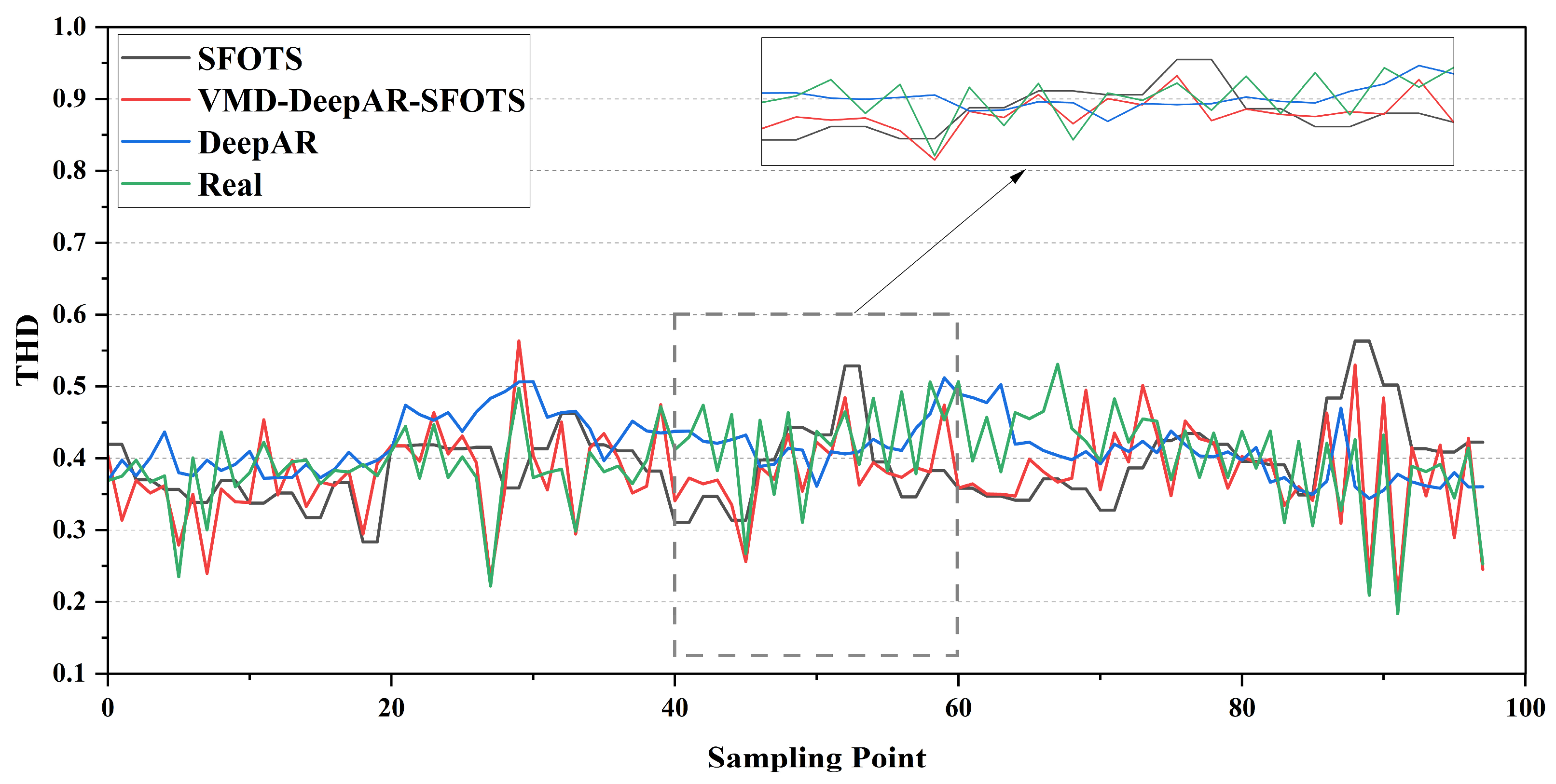
Figure 21.
Performance Comparison of ablation Models.
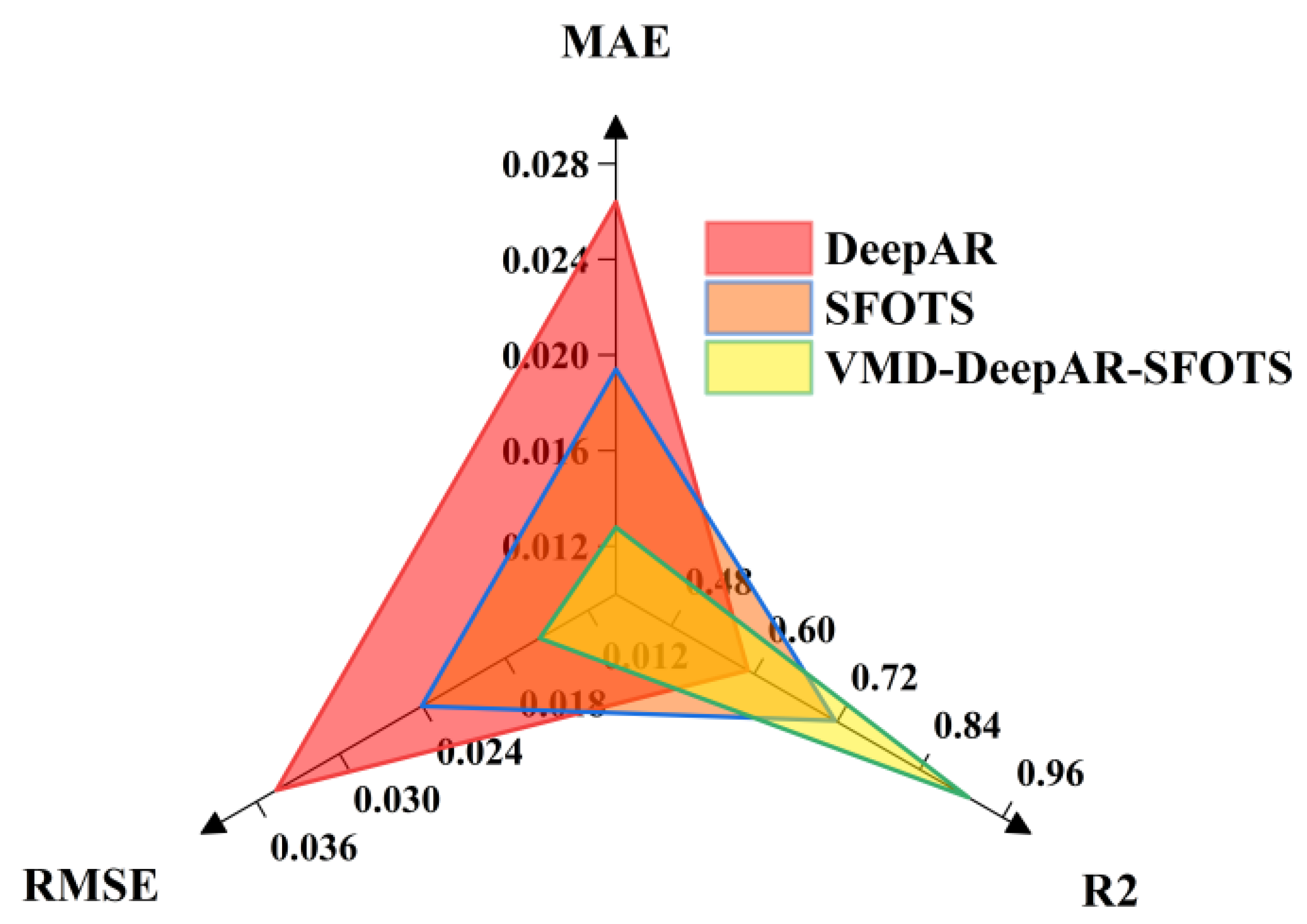

Table 1.
Optimal prediction models with different components.
| Signal | Model | R-Square | RMSE | MAE |
| IMF0 | DeepAR | 0.9026 | 0.0058 | 0.0052 |
| IMF1 | DeepAR | 0.8253 | 0.0144 | 0.0068 |
| IMF2 | SOFTS | 0.9650 | 0.0027 | 0.0022 |
| IMF3 | SOFTS | 0.9456 | 0.0019 |
0.0017 |
| IMF4 | SOFTS | 0.9531 | 0.0019 |
0.0015 |
| IMF5 | SOFTS | 0.9518 | 0.0017 |
0.0013 |
| IMF6 | SOFTS | 0.9630 | 0.0016 |
0.0013 |
| IMF7 | SOFTS | 0.9610 | 0.0015 | 0.0011 |
| IMF8 | SOFTS | 0.9790 | 0.0013 | 0.0010 |
| IMF9 | SOFTS | 0.9942 | 0.0009 | 0.0007 |
Table 2.
Comparative experimental results.
| Model | MAE | R2 | RMSE |
| LightGBM | 0.038265 | 0.363053 | 0.051082 |
| XGBoost | 0.044718 | 0.11304 | 0.060279 |
| CatBoost | 0.038634 | 0.370443 | 0.050875 |
| SVR | 0.035736 | 0.435446 | 0.048092 |
| RF | 0.04221 | 0.237514 | 0.05589 |
| MLP | 0.038717 | 0.28525 | 0.054112 |
| DT | 0.044227 | 0.184848 | 0.057786 |
| ELM | 0.032125 | 0.517995 | 0.044437 |
| Bay | 0.041688 | 0.287184 | 0.054039 |
| KNN | 0.046225 | 0.093730 | 0.060932 |
| GBR | 0.042728 | 0.237531 | 0.055889 |
| VMD-DeepAR-SOFTS | 0.0128 | 0.9099 | 0.015523 |
Table 3.
Results of ablation experiments.
| Model | MAE | R2 | RMSE |
| DeepAR | 0.0264 | 0.5909 | 0.03457 |
| SOFTS | 0.0194 | 0.7173 | 0.02405 |
| VMD-DeepAR-SOFTS | 0.0128 | 0.9099 | 0.015523 |
Table 4.
Generalization experiments.
| The collected data set | MAE | R² | RMSE |
| 1 | 0.0131 | 0.9123 | 0.0157 |
| 2 | 0.0125 | 0.9085 | 0.0154 |
| 3 | 0.013 | 0.911 | 0.0156 |
| 4 | 0.0127 | 0.9102 | 0.0155 |
| 5 | 0.0129 | 0.9095 | 0.0155 |
| 6 | 0.0132 | 0.913 | 0.0158 |
| 7 | 0.0126 | 0.9078 | 0.0153 |
| 8 | 0.013 | 0.912 | 0.0156 |
| 9 | 0.0128 | 0.91 | 0.0155 |
| 10 | 0.0129 | 0.9115 | 0.0155 |
Disclaimer/Publisher’s Note: The statements, opinions and data contained in all publications are solely those of the individual author(s) and contributor(s) and not of MDPI and/or the editor(s). MDPI and/or the editor(s) disclaim responsibility for any injury to people or property resulting from any ideas, methods, instructions or products referred to in the content. |
© 2026 by the authors. Licensee MDPI, Basel, Switzerland. This article is an open access article distributed under the terms and conditions of the Creative Commons Attribution (CC BY) license (http://creativecommons.org/licenses/by/4.0/).
Copyright: This open access article is published under a Creative Commons CC BY 4.0 license, which permit the free download, distribution, and reuse, provided that the author and preprint are cited in any reuse.


