
Submitted:
23 February 2026
Posted:
28 February 2026
You are already at the latest version
Abstract
Active vibration control is crucial for mitigating harmful resonant vibrations in structures subjected to harmonic loads. While antiresonant (zero-placement) methods are effective for this purpose, existing state-feedback solutions require full state measurement, and output-feedback approaches often prioritize resonance assignment over direct harmonic cancellation. This work bridges the gap by proposing a novel systematic design for a Proportional-Derivative (PD) output-feedback controller to achieve antiresonance. The method first computes a homogeneous stabilizing gain solution. It then leverages the parametrization of all antiresonant solutions as a constraint within a genetic algorithm optimization. The algorithm optimizes both the stability margin, characterized by an Ms-disk criterion, and the number of encirclements of the critical point $(-1,0)$ in the complex plane, as assessed by the Generalized Nyquist Stability Criterion. The proposed approach provides a practical, optimized output-feedback strategy for precise rejection of harmonic disturbances, as demonstrated through three numerical examples from real-world applications. The results confirm the method's effectiveness in synthesizing stabilizing controllers that enforce antiresonance while ensuring robust stability margins.
Keywords:
output feedback
; vibration control
; time-delay
; zero assignment
; Nyquist criterion
; optimization
; stability margin
1. Introduction
1.1. Motivation
Mechanical vibration of structural systems is a ubiquitous phenomenon across various contexts and real-world applications. In industrial processes, piping, chimneys, compressor and pump bases, for example, are among the structures that can experience harmful vibrations due to harmonic loads and perturbations [1,2,3,4,5,6]. Possible causes include gust winds, earthquakes, misalignment, and flux pulsation; they can induce resonance with the structure’s natural frequencies. To mitigate the effects of harmonic loads, passive [7,8], semi-active [9,10], and active techniques [11] can be used. Passive or semi-active techniques have some disadvantages, such as being generally ad hoc and addressing only localized vibrations, although they are inexpensive. Active vibration control methods based on linear dynamic models are more costly to implement but are flexible and can mitigate vibrations across the structure. Active vibration control methods include resonant and antiresonant approaches. In the resonant case, a prescribed location - strict or regional for the system eigenstructure is determined by the designer, and feedback controllers, as state-feedback [12,13,14], output feedback - static or dynamic [15,16], are computed to achieve the specified spectrum or eigenstructure. Antiresonant methods are designed to address the so-called harmonic loads or perturbations. In that case, a harmonic excitation enters the system in a given degree of freedom, and the goal is to cancel its effect in steady-state on another target degree of freedom of relevance. To achieve this, zeros are placed at the chosen impedance. Since the seminal work [17], a series of prominent contributions for antiresonance or zero placement using system frequency response - also known as receptance - have been made to the state of the art, as summarized in the next subsection.
1.2. State of the Art
The harmonic perturbation decoupling was initially characterized by Mottersehead et al. [7,17], who proposed zero-placement conditions and a formulation for single-input systems based on system receptance. Subsequently, several contributions were made, including the extension to multi-input systems and the concept of an adjunct system [18] . For systems with delay, a recent work [19] synergises the results with the Nyquist stability criterion explored in [14,20,21], incorporating time delays in the measurements. In that work, state-feedback controllers are designed, which demand the full state measurement - displacements and velocities. Output feedback for an antiresonant optimized design was proposed in [22] using displacement and velocity measurements. The use of output feedback PD controllers for active vibration control in systems with actuation delays to cancel harmonic perturbations is, to the best of our knowledge, a novel solution.
1.3. Contribution of This Work and Paper Organization
In this paper, the antiresonant/zero placement is proposed by computing a proportional-derivative (PD) output feedback controller that matches closed-loop stability based on the Generalized Nyquist Stability Criterion [23]. To this end, a homogeneous solution for the proportional and derivative feedback gains that stabilizes the system is computed. Then, the parametrization of all antiresonant solutions is used as a constraint in a genetic algorithm search for an optimal solution that minimizes the stability margins represented by an -disk and the number of encirclements of the critical point in the complex plane [24,25]. The rest of the paper as organized as: (i) Section 2 presents the preliminary concepts and gives the statement of the problem to be solved; (ii) Section 3 describes the proposed approach to the output feedback PD controller design in a systematic way; (iii) Section 4 presents the numerical examples borrowed from real world application to illustrate the proposal; (iv) Section 5 outline a brief discussion on the results and the advantages/drawback of the proposal; (v) and Section 6 presents some conclusions and perspectives.
2. Preliminaries and Statement of the Problem
Let the second order linear, n-DOF system be defined as:
in which are, respectively, the mass, damping, and stiffness matrices; is the influence matrix for the control input ; are standard vectors of dimension n; is a harmonic disturbance; is the sensing (measurement) matrix that defines the measurement output vector ; and is the p-th DOF of the system.
For the statement of the problem, the approach will be considered using a proportional-derivative (PD) output feedback solution of the form:
with . If the input vector is subject to fixed time delays of (possibly) different values, then by taking the Laplace Transform with relaxed initial conditions, one can write in the frequency domain the following relation:
in which the delay diagonal matrix is given as:
The antiresonant control for this closed-loop dynamics can then be stated as:
Problem 1.
In summary, the influence of the harmonic disturbance entering the system throughout the p-th DOF over the displacement of the q-th DOF is perfectly canceled at the steady-state with the computed PD output feedback controller.
3. The Proposed Approach
3.1. Zero Assignment
By developing (5), one can find the frequency domain generalized displacement:
from witch left-multiplying by gives:
The matrix is the well-known closed-loop receptance. Notice that for annihilation of at steady-state, as required in the Problem 2.1, an undamped complex zero pairs must be zeros of the cross-receptance . Let be the closed-loop dynamic stiffness matrix of the controlled system, that is:
Thus, the receptance can then be written as:
in which is de adjoint matrix of the dynamic stiffness. As can be found in [26], this matrix has, by construction, the entries given by:
In the above equation, is the minor, computed after the deletion of the q-th row and p-th column of the dynamic stiffness matrix. Notice that the zeros of are the roots of the equation:
Denoting the basis for the right null spaces of the standard vectors and , respectively, as the matrices and , it can be verified that:
with:
The dynamic stiffness matrix and its respective matrices above are called the adjunct system ofr (1). The poles of the associated receptance are the zeros of . In summary, to proceed with the zero assignment that is a solution for problem 2.1, the pole assignment of must be performed.
Focusing now in the for pole assignment, one has:
The Sherman-Morrison-Woodbury formula can be applied to expanding this inverse, resulting in:
with . The characteristic equation for (17) is given as:
In order to assign a set of roots to this equation, say, in closed-loop, since is a closed loop pole of the system, then:
This is equivalent to state that the rank of the matrix:
is equal to . If one picks a vector from the null space of , says, , then the following result is true:
Expanding this, one has:
Applying the `vec-trick’ to the above equation and casting for results in:
Such a system can be written in a compact form as , with an obvious definition of the system matrices. This is a linear system with equations, dictated by the number of zeros to be assigned and the dimension of the measurement vector, and unknowns, the elements of the feedback gain matrices. Some facts regarding the system solutions are:
- (i)
- The system has solutions if for all nontrivial vector , , that is, is full row rank;
- (ii)
- If this condition is matched, the number of free variables in the solution is ;
- (iii)
Notice that any solution computed using (19) can be used as the homogeneous in (20). As an instance, the Moore-Penrose inverse can be applied to compute:
Other generalized inverses can be used to compute .
3.2. Optimization-Based Solution
The parametrization of all-antiresonant feedback matrices (20) gives the designer the possibility of exploring the free parameter for seeking in an in general large space of dimension [18,27]. An indispensable requirement is that the solution must give a stable closed-loop system. Several works using state or state-derivative feedback controllers [19,20,21] addressed this issue using the Nyquist stability criterion [28], or its generalized version for the multi-input case [23]. The closed-loop receptance can be deduced as:
The closed-loop poles of (22) are the roots of the characteristic equation:
where is the so-called loop gain function of the controlled system. Lemma 1 in Appendix A.1 establishes the conditions for the closed-loop system to be stable according to the Generalized Nyquist Criterion. Thus, given a prescribed value of that imposes delay and gain margins for the closed-loop system, and by considering a frequency range sufficient large far from the highest natural frequency of the open-loop poles, , the following optimization problem can be solved to compute the feedback gain matrices and :
4. Numerical Studies
4.1. Test Cases Description
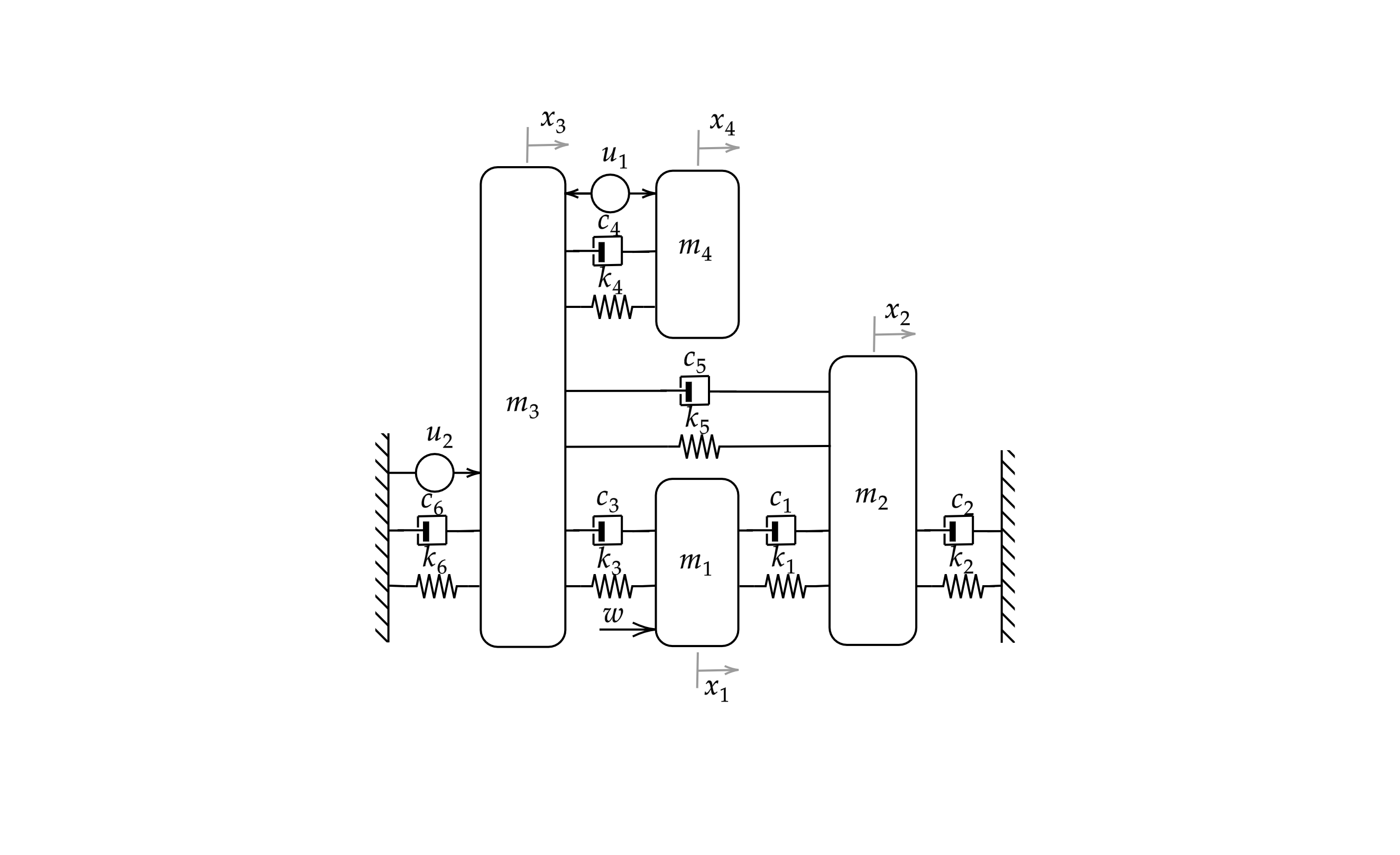
Three examples demonstrate the effectiveness of PD controllers for antiresonance performance when the proposed approach is applied. In the first one, a spring-mass-damper with four DOF, two control inputs, and two measured displacements in a collocated sensor-actuator scheme is studied. Such an example can model several kinds of structural systems. In the second example, an unstable open-loop model for the friction-induced vibration phenomenon in a belt conveyor with a structural contact point is employed to illustrate the proposed antiresonant design. The third example is a reduced-order model of a building with active vibration control applied to two target harmonic disturbance frequencies.
4.1.1. Case I: Collocated Sensors and Actuators in a Structural System
This example illustrates the antiresonant design of a 4-DOF mass-spring-damper, as shown in Figure 1. The harmonic perturbation , with enters in the 1st DOF, and must be suppressed in the 2nd DOF, that is:
The system mass, damping, and stiffness matrices together with the influence matrix were borrowed from the experimental assembly [22], and considering a collocated measurement, are given as:
The delays at the input are considered as s. An -disk with radius , that is, , is chosen to the design. The system is open-loop stable, that is, ; then, the encirclements of the critical point must be null. A stabilizing homogeneous solution is computed using the parameters:
The feedback matrices were computed, resulting:
The Nyquist contour with the fixed disk is depicted in Figure 2, and the system stability can be certified using this visualization: no encirclements are observed in the plot. The time domain responses of the target DOF for harmonic disturbance rejection and the control effort demanded are displayed respectively in Figure 3 and Figure 4.
4.1.2. Case II: Non-Collocated Sensors and Actuators Control of System with Friction-Induced Vibration
In this test case, the well-known friction-induced vibration phenomenon [29] is visited, in an example borrowed from [30]. The mechanical system is displayed in Figure 5. The belt movement creates friction at the contact point, and depending on the friction coefficient, unstable vibration can occur. For design purposes, the system matrices for this system are the following:
Input delays are given as s, , and . The system has an unstable pair of eigenvalues, namely, , that is . An harmonic perturbation , with enters the system in the second DOF, and the effect at itself, that is, the point inertance must have an annihilator zero pair . Thus, one has:
As in the previous Test Case, is adopted. A stabilizing homogeneous solution is computed using the parameters:
The feedback gain matrices are then computed, resulting:
In Figure 6, the generalized Nyquist contour resulting from the computed controller is displayed, in full view and in detail. It is evident that the double crossing of the critical point of the complex plane corresponds to . A simulation in which the loop is closed in the instant was performed. The effectiveness of the controller can be checked in Figure 7, which shows the time-domain response of the target DOF, and in Figure 8, where the control effort delivered by the designed controller is depicted.
4.1.3. A Reduced Model of a Hospital Building
In this example, a reduced-order model of a four-DOF hospital building [31,32] is used for antiresonant design. A collocated sensor-actuator is used as in the case Section 4.1.1. The system matrices are:
Input delays are s, s, and s. The system is open-loop stable, that is . An harmonic perturbation with two mixed frequencies , with and enters the system in the first DOF, and the effect at third DOF, that is, the cross inertance must have two annihilator zero pairs and . Thus, one has:
The disk for the margins definition has . A stabilizing homogeneous solution is computed using the parameters:
The feedback gain matrices are then computed, resulting:
In Figure 9, the generalized Nyquist contour resulting from the computed controller is displayed, in full view and in detail. It is evident there is no crossing of the critical point of the complex plane, corresponding to . A simulation in which the loop is closed in the instant was performed. The effectiveness of the controller can be checked in Figure 10, which shows the time-domain response of the target DOF, and in Figure 11, where the control effort delivered by the designed controller is depicted.
4.2. Robustness Margins
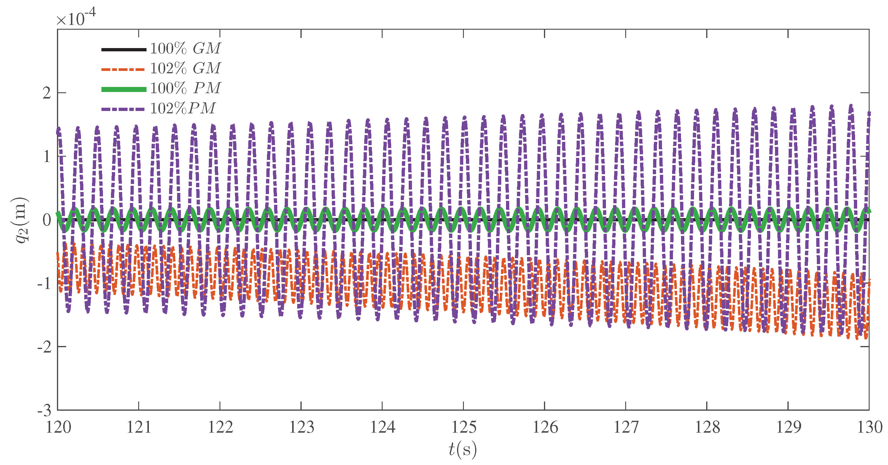
To illustrate the closed-loop system margins of the design described in the Appendix A.2, the test case Section 4.1.1 is stressed to the margins and slightly beyond that. The effective margins of the system were computed from the eigenloci as:
To introduce the phase margin in the simulation, the critical frequency was identified as rad/s, resulting in a maximum additional delay in the loop of s. The simulations were running with no perturbations and an initial displacement of . The displacement of the target DOF is displayed in Figure 12. The system is resilient and exhibits marginal stability with of the computed margins, introduced once at a time. The uncertainty was increased beyond those values, leading to , and the closed-loop unstable behaviors are then noted.
5. Discussion
The proposed approach to antiresonant control has been demonstrated to be effective in silencing the effect on a chosen DOF of harmonic perturbations entering the system in a given DOF. That is the better strategy to mitigate perturbations rather than the resonant-pole assignment design. Another relevant point is that, although in the examples the system matrices are known, the proposal can leverage experimental identification of the system receptance [17,33] and, subsequently, the dynamic stiffness matrix to handle the adjoint system for zero assignment. Moreover, the use of proportional-derivative output feedback further enhances the approach’s advantages, as only displacement sensors are required, whereas in [22] velocity measurements are used for feedback. Yet, related to this work, the proposed approach can handle multiple perturbation frequencies rather than a single frequency as in [22]. The same can be said of the multiple delays considered here, whereas a single delay is explored in [22].
6. Conclusions
This paper presented a novel systematic approach for designing PD output-feedback controllers to achieve antiresonance in second-order mechanical systems subjected to harmonic disturbances. By formulating the zero assignment problem as a pole assignment of an adjoint system, the method enables direct cancellation of harmonic components at target degrees of freedom. The proposed optimization framework integrates stability constraints via the Generalized Nyquist criterion and -disk robustness margins, with a genetic algorithm exploring the solution space.
The effectiveness of the methodology was demonstrated through three numerical examples encompassing collocated and non-collocated configurations, stable and unstable open-loop systems, and multiple disturbance frequencies. Results confirm that stabilizing controllers enforcing antiresonance while ensuring robust stability margins can be systematically synthesized.
Future work will focus on experimental validation, extension to nonlinear systems, and integration with data-driven identification techniques to bypass explicit model requirements. Additionally, investigating adaptive schemes for time-varying disturbance frequencies and exploring alternative optimization algorithms may further enhance the practical applicability of the proposed approach.
Author Contributions
Conceptualization, J.M.A., J.R.B.A, N.J.B.D. and C.E.T.D.; methodology, J.M.A. and C.E.T.D.; software, J.M.A. and N.J.B.D.; validation, J.M.A., J.R.B.A, N.J.B.D. and C.E.T.D.; formal analysis, J.M.A., and C.E.T.D.; investigation, J.M.A., J.R.B.A, N.J.B.D. and C.E.T.D.; resources, J.M.A., and C.E.T.D.; data curation, J.M.A.; writing—original draft preparation, J.M.A., J.R.B.A, N.J.B.D. and C.E.T.D.; writing—review and editing, J.M.A. and C.E.T.D.; visualization, J.M.A.; supervision, J.M.A. and C.E.T.D.; project administration, J.M.A. and C.E.T.D.; funding acquisition, J.M.A. and C.E.T.D. All authors have read and agreed to the published version of the manuscript.
Funding
This research was funded by Conselho Nacional de Desenvolvimento Científico e Tecnológico - CNPq grant numbers: 311478/2022–0 and 306178/2023–0
Data Availability Statement
The raw data supporting the conclusions of this article will be made available by the authors on request.
Conflicts of Interest
The authors declare no conflicts of interest.
Appendix A
Appendix A.1
The Lemma presented here can be found in [19], and the complete proof is presented in [23]. Let be the loop function, as defined in Section 3.2:
Assume that the characteristic equation has roots - open-loop poles - in the right half-plane. Setting , in which is the frequency, the Generalized Nyquist criterion can be enounced with the help of the following definitions.
Definition A1.
The eigenloci is the set of all the geometric branches, in the complex plane, obtained by computing the eigenvalues , when ω varies in the interval of frequencies , with .
Definition A2.
The number of counterclockwise encirclements of the point by the k-th branch of the eigenloci in the complex plane is denoted as .
Definition A3.
The number of counterclockwise encirclements of the point by the k-th branch of the eigenloci in the complex plane is denoted as .
Assumption A1.
The eigenloci of the loop function has no clockwise encirclements of the critical point , that is, .
Lemma A1.
The closed-loop system in Equation (22) with Assumption 1 is exponentially stable iff:
- 1.
- ;
- 2.
- .
Appendix A.2. System Margins from the Nyquist Contour
For a controller design that assures the Nyquist contour outside the called disk, the following bounds for gain margin and phase margin can be certified for open-loop stable models [24]:
References
- Cheng, Y.; Dai, K.; Liu, Y.; Yang, H.; Sun, M.; Huang, Z.; Camara, A.; Yin, Y. A method for along-wind vibration control of chimneys by tuning liners. Engineering Structures 2022, 252, 113561. [Google Scholar] [CrossRef]
- Menon, D.; Rao, P. Estimation of along-wind moments in RC chimneys. Engineering Structures 1997, 19, 71–78. [Google Scholar] [CrossRef]
- Zeng, X.; Xu, J.; Han, B.; Zhu, Z.; Wang, S.; Wang, J.; Yang, X.; Cai, R.; Du, C.; Zeng, J. A Review of Linear Compressor Vibration Isolation Methods. Processes 2024, 12. [Google Scholar] [CrossRef]
- Liu, S.; Gu, C.; Tian, Q.; Huang, D.; Guo, Y. Research on the vibration mechanism of compressor complex exhaust pipeline based on transient flow. International Journal of Hydrogen Energy 2025, 139, 886–894. [Google Scholar] [CrossRef]
- Matin Nikoo, H.; Bi, K.; Hao, H. Passive vibration control of cylindrical offshore components using pipe-in-pipe (PIP) concept: An analytical study. Ocean Engineering 2017, 142, 39–50. [Google Scholar] [CrossRef]
- Ding, H.; Ji, J.C. Vibration control of fluid-conveying pipes: A state-of-the-art review. Applied Mathematics and Mechanics 2023, 44, 1423–1456. [Google Scholar] [CrossRef]
- Mottershead, J.E.; Ram, Y.M. Inverse eigenvalue problems in vibration absorption: Passive modification and active control. Mechanical Systems and Signal Processing 2006, 20, 5–44. [Google Scholar] [CrossRef]
- Richiedei, D.; Trevisani, A. Simultaneous active and passive control for eigenstructure assignment in lightly damped systems. Mechanical Systems and Signal Processing 2017, 25, 556–566. [Google Scholar] [CrossRef]
- Ikeda, Y. Active and semi-active vibration control of buildings in Japan – Practical applications and verification. Structural Control and Health Monitoring 2009, 16, 703–723. [Google Scholar] [CrossRef]
- Dyke, S. Acceleration Feedback Control Strategies for Active and Semi-active Control Systems: Modeling, Algorithm Development, and Experimental Verification. PhD thesis, University of Notre Dame, 1996. [Google Scholar]
- Ouyang, H.; Wei, X.; Mottershead, J.E. Structural modification and active vibration control by the receptance method: Review and tutorial. Mechanical Systems and Signal Processing 2025, 241, 113532. [Google Scholar] [CrossRef]
- Ram, Y.; Singh, A.; Mottershead, J.E. State feedback control with time delay. Mechanical Systems and Signal Processing 2009, 23, 1940–1945. [Google Scholar] [CrossRef]
- Araújo, J.M.; Dórea, C.E.; Gonçalves, L.M.; Datta, B.N. State derivative feedback in second-order linear systems: A comparative analysis of perturbed eigenvalues under coefficient variation. Mechanical Systems and Signal Processing 2016, 76–77, 33–46. [Google Scholar] [CrossRef]
- Araújo, J.M. Discussion on ’State feedback control with time delay’. Mechanical Systems and Signal Processing 2018, 98, 368–370. [Google Scholar] [CrossRef]
- Bernstein, D.S.; Bhat, S.P. Lyapunov Stability, Semistability, and Asymptotic Stability of Matrix Second-Order Systems. Journal of Mechanical Design 1995, 117, 145–153. [Google Scholar] [CrossRef]
- Araújo, J.M.; Castelan, E.d.B.; Dórea, C.E.T.; Isidório, I.D. A bilinear optimization-based approach for eigenstructure assignment output feedback control of second-order linear systems. Research Square 2025. [Google Scholar] [CrossRef]
- Mottershead, J.E.; Ram, Y.M. Receptance Method in Active Vibration Control. AIAA Journal 2007, 45, 562–567. [Google Scholar] [CrossRef]
- Richiedei, D.; Tamellin, I.; Trevisani, A. Pole-zero assignment by the receptance method: Multi-input active vibration control. Mechanical Systems and Signal Processing 2022, 172, 108976. [Google Scholar] [CrossRef]
- Araújo, J.M.; Dantas, N.J.; Dórea, C.E.; Richiedei, D.; Tamellin, I. Pole-zero placement through the robust receptance method for multi-input active vibration control with time delay. Journal of Sound and Vibration 2025, 599, 118850. [Google Scholar] [CrossRef]
- Araújo, J.M.; Bettega, J.; Dantas, N.J.B.; Dórea, C.E.T.; Richiedei, D.; Tamellin, I. Vibration Control of a Two-Link Flexible Robot Arm with Time Delay through the Robust Receptance Method. Applied Sciences 2021, 11, 9907. [Google Scholar] [CrossRef]
- Dantas, N.J.B.; Dorea, C.E.T.; Araujo, J.M. Partial pole assignment using rank-one control and receptance in second-order systems with time delay. Meccanica 2021, 56, 287–302. [Google Scholar] [CrossRef]
- Saldanha, A.; Michiels, W.; Kuře, M.; Bušek, J.; Vyhlídal, T. Stability optimization of time-delay systems with zero-location constraints applied to non-collocated vibration suppression. Mechanical Systems and Signal Processing 2024, 208, 110886. [Google Scholar] [CrossRef]
- Desoer, C.; Wang, Y.T. On the generalized nyquist stability criterion. IEEE Transactions on Automatic Control 1980, 25, 187–196. [Google Scholar] [CrossRef]
- Skogestad, S.; Postlethwaite, I. Multivariable Feedback Control: Analysis and Design; Wiley, 2005. [Google Scholar]
- Sebek, M.; Hurák, Z. An often missed detail: Formula relating peek sensitivity with gain margin less than one. In Proceedings of the 17th International Conference on Process Control ’09, 2009; pp. 1–9. [Google Scholar]
- Bernstein, D. Matrix Mathematics: Theory, Facts, and Formulas (Second Edition); Princeton reference, Princeton University Press, 2009. [Google Scholar]
- Belotti, R.; Richiedei, D. Pole assignment in vibrating systems with time delay: An approach embedding an a-priori stability condition based on Linear Matrix Inequality Special issue on control of second-order vibrating systems with time delay. Mechanical Systems and Signal Processing 2020, 137, 106396. [Google Scholar] [CrossRef]
- Nyquist, H. Regeneration theory. The Bell System Technical Journal 1932, 11, 126–147. [Google Scholar] [CrossRef]
- Popp, K. Modelling and control of friction-induced vibrations. Mathematical and Computer Modelling of Dynamical Systems 2005, 11, 345–369. [Google Scholar] [CrossRef]
- Liang, Y.; Yamaura, H.; Ouyang, H. Active assignment of eigenvalues and eigen-sensitivities for robust stabilization of friction-induced vibration. Mechanical Systems and Signal Processing 2017, 90, 254–267. [Google Scholar] [CrossRef]
- Chahlaoui, Y.; Van Dooren, P. Benchmark Examples for Model Reduction of Linear Time-Invariant Dynamical Systems. In Proceedings of the Dimension Reduction of Large-Scale Systems; Benner, P., Sorensen, D.C., Mehrmann, V., Eds.; Berlin, Heidelberg, 2005; pp. 379–392. [Google Scholar]
- Betcke, T.; Higham, N.J.; Mehrmann, V.; Schröder, C.; Tisseur, F. NLEVP: A Collection of Nonlinear Eigenvalue Problems. ACM Transaction on Mathematical Software 2013, 39, 7:1–7:28. [Google Scholar] [CrossRef]
- Mottershead, J.E.; Tehrani, M.G.; James, S.; Court, P. Active vibration control experiments on an AgustaWestland W30 helicopter airframe. Proceedings of the Institution of Mechanical Engineers, Part C: Journal of Mechanical Engineering Science 2012, 226, 1504–1516. [Google Scholar] [CrossRef]
Figure 1.
Mechanical system with 4 DOF of the test case Section 4.1.1
Figure 1.
Mechanical system with 4 DOF of the test case Section 4.1.1
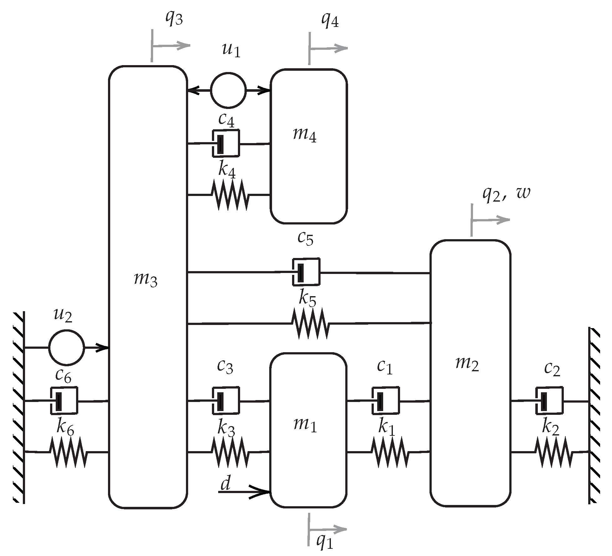
Figure 2.
Generalized Nyquist contour for the closed-loop system of the test case Section 4.1.1
Figure 2.
Generalized Nyquist contour for the closed-loop system of the test case Section 4.1.1
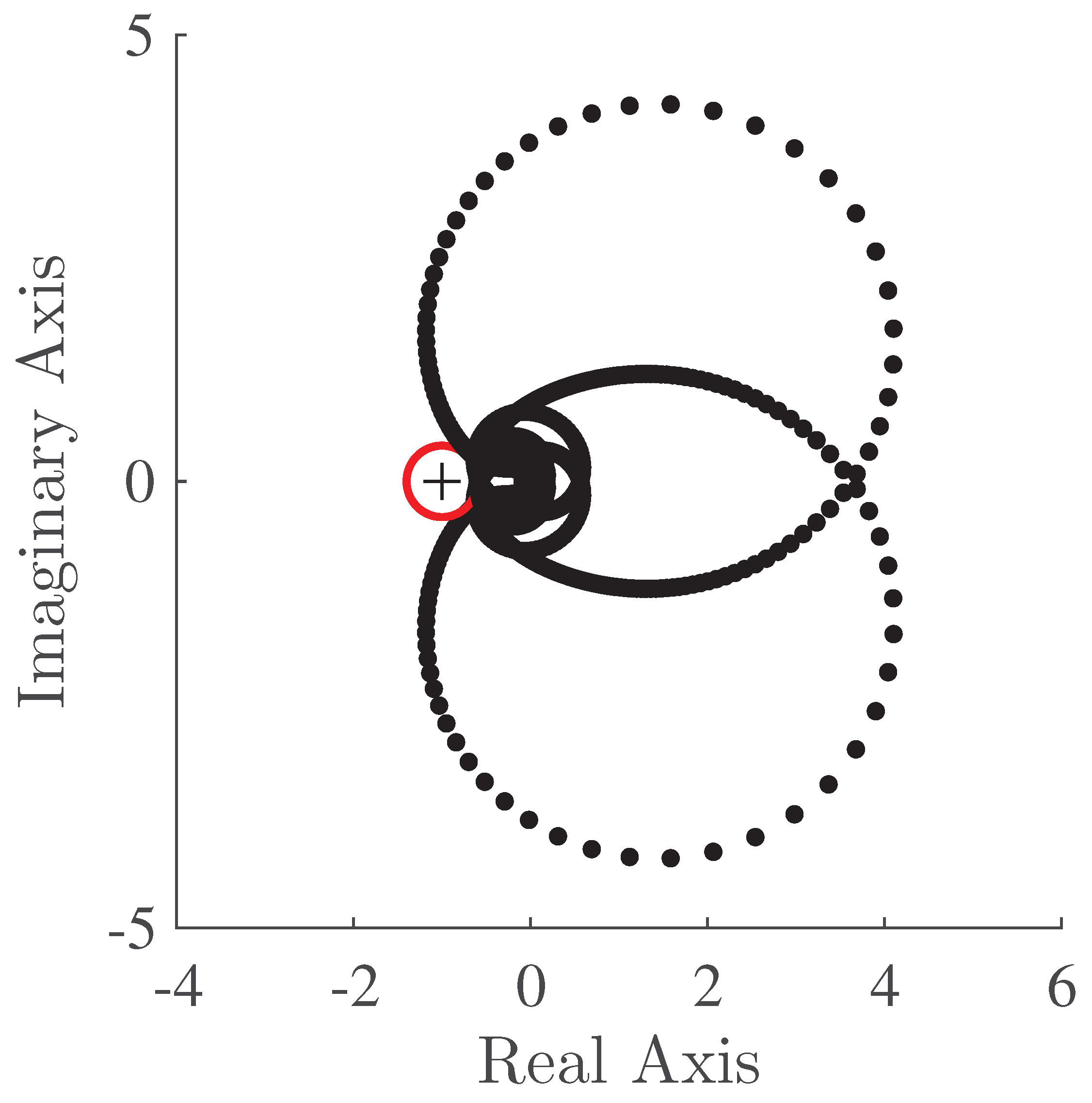
Figure 3.
Time domain response of the target DOF before and after the loop closing.
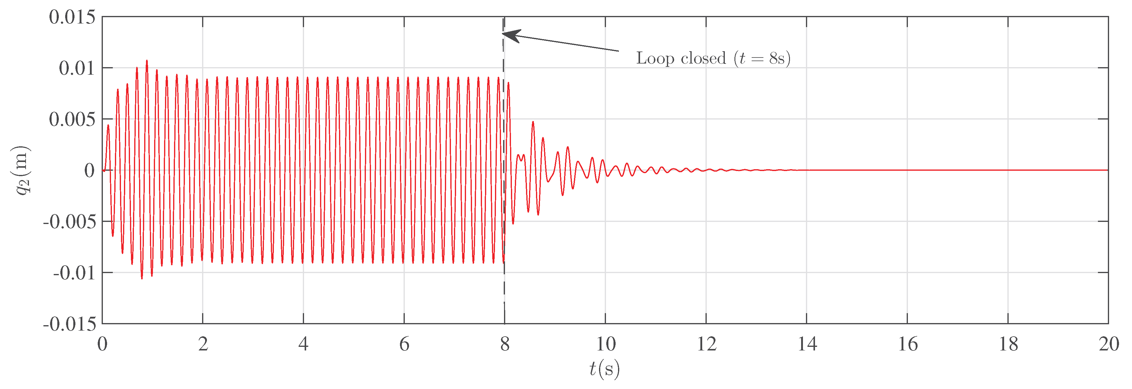
Figure 4.
Control effort of the test case Section 4.1.1
Figure 4.
Control effort of the test case Section 4.1.1
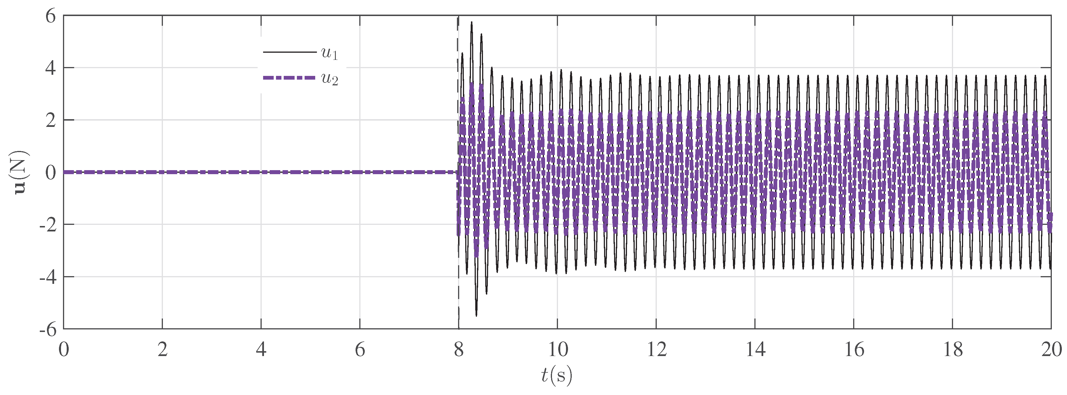
Figure 5.
Friction-induced vibration system
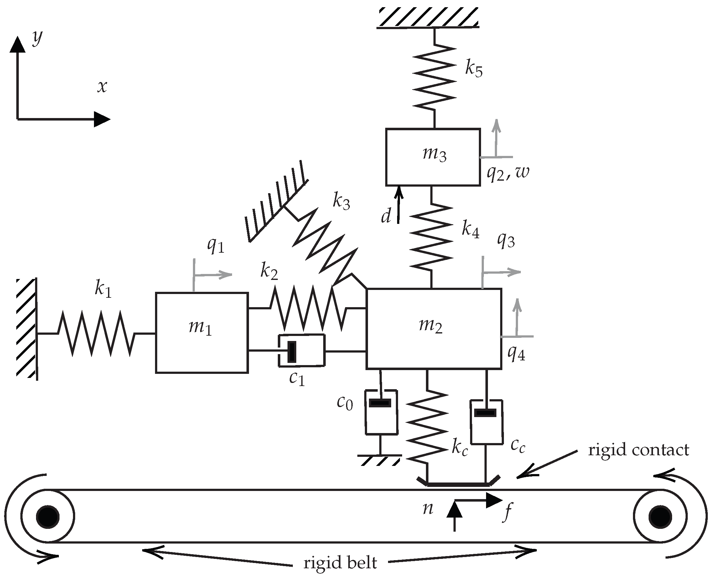
Figure 6.
Generalized Nyquist contour for the closed-loop system of the test case Section 4.1.2
Figure 6.
Generalized Nyquist contour for the closed-loop system of the test case Section 4.1.2
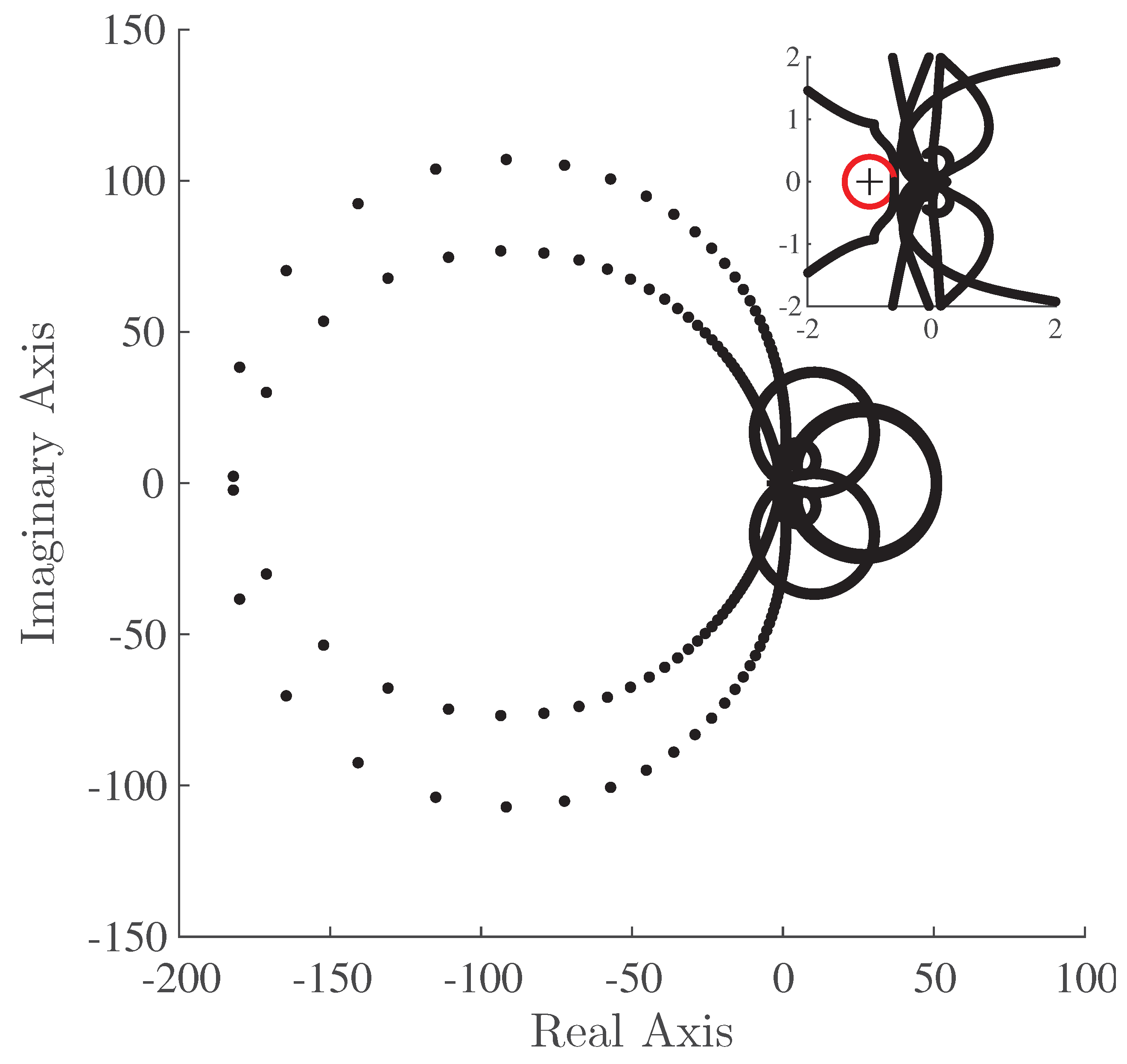
Figure 7.
Time domain response of the target DOF before and after the loop closing.
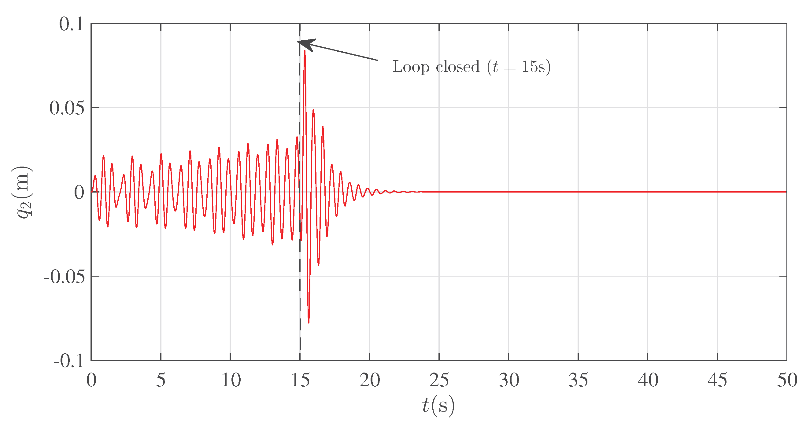
Figure 8.
Control effort of the test case Section 4.1.2
Figure 8.
Control effort of the test case Section 4.1.2
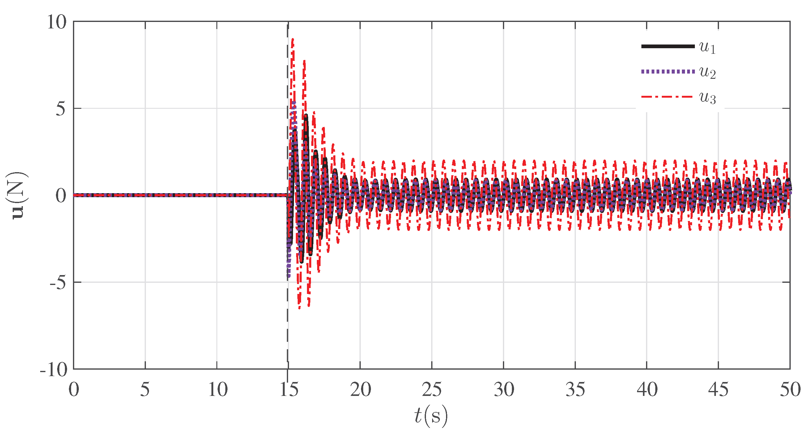
Figure 9.
Generalized Nyquist contour for the closed-loop system of the test case Section 4.1.3
Figure 9.
Generalized Nyquist contour for the closed-loop system of the test case Section 4.1.3
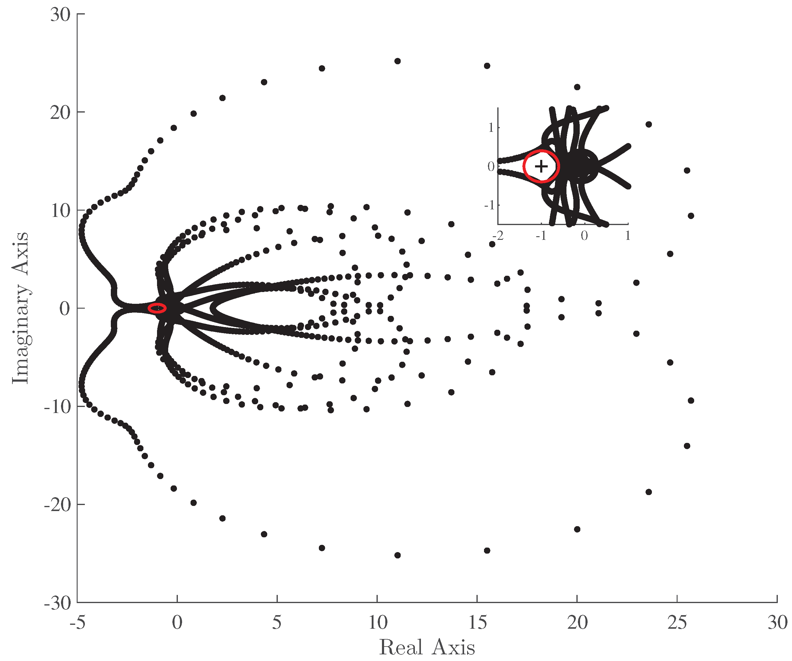
Figure 10.
Time domain response of the target DOF before and after the loop closing.
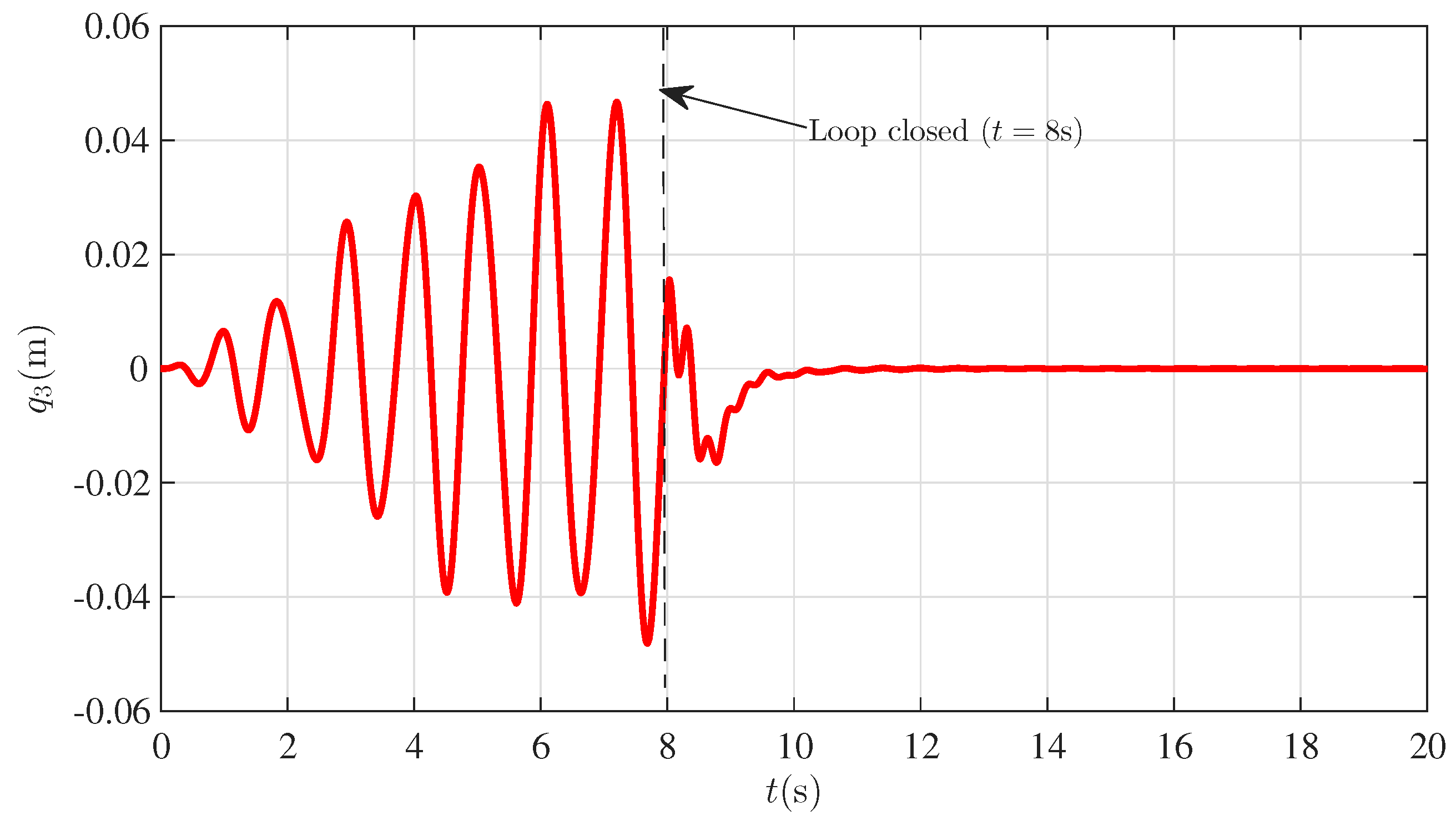
Figure 11.
Control effort of the test case Section 4.1.3
Figure 11.
Control effort of the test case Section 4.1.3
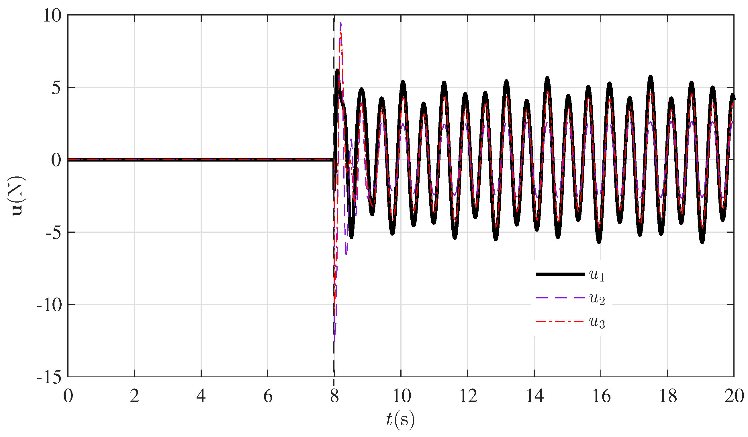
Figure 12.
Closed-loop response of test case Section 4.1.1 with gain and phase stressed on and beyond the margins.
Figure 12.
Closed-loop response of test case Section 4.1.1 with gain and phase stressed on and beyond the margins.
Disclaimer/Publisher’s Note: The statements, opinions and data contained in all publications are solely those of the individual author(s) and contributor(s) and not of MDPI and/or the editor(s). MDPI and/or the editor(s) disclaim responsibility for any injury to people or property resulting from any ideas, methods, instructions or products referred to in the content. |
© 2026 by the authors. Licensee MDPI, Basel, Switzerland. This article is an open access article distributed under the terms and conditions of the Creative Commons Attribution (CC BY) license (http://creativecommons.org/licenses/by/4.0/).
Copyright: This open access article is published under a Creative Commons CC BY 4.0 license, which permit the free download, distribution, and reuse, provided that the author and preprint are cited in any reuse.


