
Submitted:
24 November 2024
Posted:
26 November 2024
You are already at the latest version
Abstract
This paper investigates the optimal control of a harmonic oscillator governed by the second-order linear equation:
$$
\ddot{x}(t) + \omega^2(t) x(t) = 0,
$$
where $x(t)$ represents the system’s position, and $\omega(t)$ is the time-varying frequency. The primary objective is to determine the minimal time T required for the system to transition from an initial state,
$x(0) = x_0,\
\dot{x}(0)=v_0$ to a final state
$
x(T) = x_T,\
\dot{x}(T) = v_T$, under the constraint that the frequency $\omega(t)$ remains a bounded function. The main challenge involves identifying the optimal switching times between two frequencies while satisfying all boundary conditions. Various boundary scenarios are analyzed, and the reachable set of all trajectories is constructed. Analytical techniques, combined with control theory and a proven theorem, are utilized to solve this problem. This study is particularly relevant for applications requiring time-optimal control, such as mechanical vibration systems or signal processing, where rapid state transitions are crucial. The methods developed provide a robust framework for time-optimal control in oscillatory systems and are adaptable to other systems facing similar control challenges.
Keywords:
optimal control
; harmonic oscillator
; Bellman optimality principle
; Pontryagin maximum principle
1. Introduction
Time-optimal control of dynamical systems is a fundamental problem in control theory, with widespread applications in engineering and physics [1,2]. This paper focuses on the optimal control of a harmonic oscillator subjected to excitation by a time-varying frequency, addressing the complexities associated with time-varying dynamics, parametric excitation, and frequency constraints. Optimal control problems involving time-dependent parameters and constraints have been extensively studied [3,4,5].However, to the best of our knowledge, the specific case of a harmonic oscillator with its frequency constrained to two discrete values, combined with the presence of viscous friction, poses a unique challenge [6,7]. Revisiting this problem, the natural question of determining the minimum time required for the system to transition between two given states was first raised in [8]. Our paper provides a comprehensive answer to that question.
The system’s dynamics are significantly affected by the switching between frequencies, making the determination of the optimal switching strategy a challenging and nontrivial task [9].
Our approach builds upon prior research in parametric excitation [10,11], where varying system parameters are employed to influence the system’s behavior, as well as on time-optimal control methods for systems with bounded control input [12,13]. An illustrative example closely related to our problem is the variable-length pendulum. In a classical pendulum, the length is fixed, resulting in a constant natural frequency. However, allowing the pendulum’s length to vary over time introduces parametric excitation, analogous to the frequency variation in the harmonic oscillator. The time-optimal control problem for the variable-length pendulum involves determining a length variation strategy that transitions the system from an initial state to a final state in minimal time.
Drawing inspiration from this analogy, we combine analytical techniques with control theory under constrained frequency parameters to develop methods for solving the optimal control problem for the harmonic oscillator. The significance of this study lies in its practical applications to systems requiring rapid state transitions under frequency constraints. For instance, in mechanical vibration systems, efficiently controlling oscillations is critical for ensuring stability and performance [14,15]. Similarly, in signal processing and communication systems, rapid frequency modulation can significantly enhance performance and adaptability [16]. In aerospace engineering and robotics, the ability to swiftly and precisely control oscillatory components within specified constraints is essential [17,18]. For example, the time-optimal control of a robotic arm with multiple joints involves solving a complex system of coupled equations, where the computational burden can become prohibitive for real-time applications. Autonomous vehicles also require near-instantaneous control adjustments to maintain safety and performance under dynamic conditions [19]. However, solving such complex optimal control problems in real time often proves infeasible due to the high computational demands. This study provides a framework to address these challenges, offering analytical and computational tools to improve the efficiency and practicality of time-optimal control solutions.
Optimal control strategies for such systems often require switching between discrete parameter values or continuously varying parameters within defined bounds. The primary challenge lies in designing a control law that minimizes the transition time while adhering to physical constraints and boundary conditions.
Previous studies have shown that efficient control strategies involve rapid adjustments of system parameters, similar to switching in harmonic oscillators. However, practical implementations must account for constraints, such as the maximum allowable rates of change, to ensure stability and prevent mechanical failure. These considerations are crucial for translating theoretical control strategies into real-world applications where robustness and safety are paramount.
In this paper, we provide a comprehensive analysis of the optimal control problem for a harmonic oscillator with frequency constraints. We investigate various boundary scenarios, construct feasible transition sets, and determine the optimal switching times between frequencies. The techniques developed in this study are adaptable to other systems facing similar control challenges, offering a robust and versatile framework for time-optimal control across a wide range of applications.
The remainder of the paper is structured as follows: Section 2: Formulation of the time-optimal control problem and discussion of mathematical preliminaries. Section 3: Development of analytical methods for determining optimal switching strategies. Section 4: Exploration of boundary scenarios with illustrative examples. Section 5: Practical implications and applications of the results. Section 6: Summary of the findings and directions for future research.
2. Preliminaries and Problem Formulation
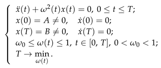
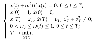
Let us consider the following optimal control problem for a harmonic oscillator
It is required to determine the control function (frequency) to transfer the system from the initial state to the final state in minimal time. It is important to note that the boundary conditions cannot be zero, as the system described by becomes uncontrollable in such cases.
This problem falls into the category of unstable bilinear optimal control problems.
In this paper, we will prove the existence of a solution to (1), outline its key properties, and present an algorithm for constructing both the optimal control and the corresponding optimal trajectory.
Remark 1.
Let us note two important properties that will be used later.
I. Let , and T be the solution to problem (1). Consider the substitution: then the function will solve the following problem
i.e., the trajectory can be scaled.
II. Let , and T be the solution to problem (1). Then the functions and will solve the following problem
with reversed time dynamics, satisfying the corresponding boundary conditions for the reversed time interval. This symmetry property can be used to simplify the analysis of the problem or construct dual solutions based on the time-reversed control and trajectory. That is, the excitation problem () and the damping problem () (see the Remark 2 to Theorem 1) of oscillations are equivalent.
In [3], a similar optimal control problem is analyzed for the specific case where :
 This scenario simplifies the boundary conditions, focusing on transferring the system between states with zero initial and final velocities. This serves as a foundational case for understanding more general boundary conditions in optimal control problems. It is demonstrated that the optimal solution to this problem exhibits an oscillatory nature, and the corresponding optimal control is a periodic function with a period equal to one semi-oscillation (Figure 1). The formulas for solving problem (2) are provided as a reference in Appendix A.
3. Solution of the Problem (1): Theoretical Analysis
The nature and structure of the solution to the optimal control problem (1), are determined by establishing a connection between the solutions of problems (1) and (2). Problem (1) addresses arbitrary initial and final velocities, while problem (2) focuses on the specific case where the initial and final velocities are zero .
Theorem 1.
For any initial conditions and and final conditions and in problem (1), the following holds: there exist constants A and B, a periodic control of the form shown in Figure 1, and a corresponding trajectory that satisfies the differential equation and boundary conditions of system (2) on some interval (where may not be the optimal), such that:
1. Existence of Key Time Points: There exist two moments in time and T () such that , , , These conditions ensure that the trajectory passes through the specified initial and final states, as illustrated in Figure 2.
Proof of Theorem 1.
The proof begins by considering a special case of the problem where . For this case, it is shown that a periodic control can be constructed to generate a trajectory satisfying the required boundary conditions. Next, the method used for this special case is extended to the general scenario with arbitrary .
I. In the case ,the scaling property of the trajectory allows the assumption and . Under this assumption, the original problem can be reformulated into the following equivalent problem:
 First, the existence of the value B in problem (2) will be established. In [3], it is demonstrated that the optimal control for problem (2) during each semi-oscillation takes the form illustrated in Figure 1. Here, denotes the duration of a single semi-oscillation, and at one of the control switching moments, or , the condition is satisfied.
Consider the reachable set of the controlled system (2) along trajectories generated by periodic controls of the form depicted in Figure 1.
First, construct the reachable set for a single semi-oscillation, which consists of the set of states that the controlled system can achieve by performing at most one semi-oscillation, starting from the initial point corresponding to the initial condition of problem (3). It is known [3] that, on individual segments where the control is constant, the optimal trajectory is always described by one of two cosine functions: for control or for control . Here, C and are constants that depend on the specific segment where the control value remains constant.
For , the trajectory on the phase plane is represented by an arc of a circle, , as the solution is . For , the trajectory becomes an arc of an ellipse, , since the solution takes the form .
The reachable set, depending on whether the amplitude of oscillations increases or decreases, is divided into two distinct parts, as shown in Figure 3. Over time, the motion along the trajectory on the phase plane consistently proceeds in a counterclockwise direction.
Figure 3 (a) illustrates oscillations with a decreasing amplitude. In this case, the second control switch occurs when the variable changes sign. As a result, in the fourth quadrant, the reachable set is bounded by two curves: an arc of the circle and an ellipse defined by . In contrast, in the third quadrant, no control switches occur, and all trajectories correspond to arcs of a circle.
Figure 3 (b) represents oscillations with an increasing amplitude. In this scenario, the first control switch occurs at the moment when the variable changes its sign. Consequently, in the fourth quadrant, the reachable set is limited to an arc of a circle. In contrast, in the third quadrant, the reachable set starts to expand, bounded by two curves: an arc of the circle and an ellipse defined by .
Similarly, construct the reachable set for two semi-oscillations (Figure 4), and by continuing in the same manner, construct the reachable set for n (n even) semi-oscillations (Figure 5).
As n approaches infinity, the reachable set expands and encompasses all points on the phase plane except for the origin.
Thus, for any given terminal point , there exists a trajectory in problem (2), generated under a specific type of control, that passes through this point at . There may be multiple such trajectories; therefore, the one with the minimal time T is chosen. Extending this trajectory to its intersection with the x-axis,yields the required value of B and the final time . Denote the selected trajectory and its corresponding control by and respectively (though this trajectory as a whole may not be optimal in problem (2)).
It has been shown that the pair , satisfies the differential equation and boundary conditions (3) on .
II. Now, it will be proven that , , () , is also a solution to the optimal control problem (3), meaning that the time T is minimal.
Assume that this is not the case. Then there exist , , , which satisfy the differential equation and the boundary conditions of problem (3) on the interval , and the time is minimal in the problem (3) (Figure 6). The optimal trajectory performs complete semi-oscillations and one final incomplete semi-oscillation. In the case where , complete semi-oscillations may be absent. Let the moments when the derivative equals zero be denoted as , and the corresponding amplitudes as , where .
According to Bellman’s principle of optimality [20], any part of the optimal trajectory is also optimal in the problem (2) or (3). Here, the autonomy of the controlled system can be utilized, meaning the coefficients are independent of time. This allows any moment in time to be considered as the initial one, not necessarily .
Thus, on each semi-oscillation, as well as on any two consecutive semi-oscillations, the trajectory satisfies all the conditions of problem (2). Using the properties [3] of the solution to problem (2), it can be concluded that, over all complete semi-oscillations, the control is a periodic function and takes the form depicted in Figure 1.
It remains to prove that on the final incomplete semi-oscillation the control has the same structure. From this, it will follow that the trajectories and coincide.
Let us consider the last incomplete semi-oscillation of the trajectory . Denote by the trajectory obtained under the control of the type shown in Figure 1, satisfying the initial conditions , , and at some moment , also satisfying the boundary conditions of problem (3): , . Here, because the trajectory is optimal (Figure 7 (a)).
Extend this trajectory up to the first moment where . If this extension is not unique, select any control of the type shown in Figure 1 and the corresponding trajectory.
The resulting trajectory will be optimal on the interval in a problem of the type (2).
Then, let us construct a new trajectory (Figure 7 (a)):
This trajectory will satisfy the same boundary conditions as the trajectory , but on a smaller interval , which contradicts the optimality of .
Hence, , and the trajectories and coincide. Consequently, the control on the interval has the same structure as shown in Figure 1.
It remains to prove that the switching points of the control on the last incomplete semi-oscillation (if they exist) coincide with the switching points on complete semi-oscillations.
Consider the last one complete and one incomplete semi-oscillation of the trajectory (Figure 7 (b)). In a similar way, it can be shown that the control on the interval also has the same structure as shown in Figure 1.
Thus, the statement of the theorem for the case is proven.
The existence of a solution to problem (1) for arbitrary values of and is proven in a similar manner. Note some minor differences. Using the scalability property of the system (1), we can assume that , meaning the initial point lies on the unit circle in the phase plane. Figure 8 shows the reachable set for no more than two semi-oscillations when the initial point is located in the first quadrant of the coordinate system. The reachable set is expanded similarly to the previous case and captures all points in the phase plane except the origin.
Thus, there exist a trajectory and a control function of the type shown in Figure 1, which satisfy the differential equation and the boundary conditions (1) on some interval .
The proof is complete. □
Remark 2.
From the proof of the theorem (see Figure 8), it follows that is non-decreasing in the case of excitation and non-increasing in the case of damping oscillations. Consequently, the boundary conditions uniquely determine the nature of the oscillations ( indicates excitation, indicates damping, and if , the oscillations have a constant amplitude).
Remark 3.
It is possible that the trajectory is not optimal on the segment . For example, Figure 9 shows the situation when the optimal trajectory (red curve) connecting the initial point and the final point extends to the intersection with the horizontal axis, and in this case the trajectory contains 3 complete semi-oscillations. But the optimal trajectory connecting the points and the endpoint contains only one semi-oscillation, since the point belongs to the reachability set for at most two semi-oscillations (area highlighted in green).
Remark 4.
Using the established periodicity of the optimal control and its specific structure, combined with the method of constructing the reachable set from the proof of Theorem 1, it is possible to plot the dependence of the optimal time in problem 1, it is possible to plot the dependence of the optimal time in problem(3) on the endpoint (Figure 10). Notably, this plot reveals a discontinuous relationship between the optimal time and the endpoint.
4. Algorithm for Constructing the Solution to Problem (1) via Reduction to a Problem with Zero Derivatives
In Section 3, Theorem 1 demonstrated that the optimal trajectory in (1) corresponds to periodic control as shown in Figure 1 over a certain time interval .
To construct the solution, it is necessary to determine the number of internal semi-oscillations (which should be minimal and may be zero), the amplitudes of the first (left) and the last (right) semi-oscillations (which may be incomplete), and the time shifts (phase shift) that define the boundary points for the solution to (1) (Figure 2, or more precisely, Figure 11). These phase shifts are relative to the points where the derivative is zero.
First Step: Determining the Amplitudes of the Initial and Final Semi-Oscillations
It is assumed that , i.e., . The case , i.e., , is analyzed similarly using Remark 1.
According to [3] (see Appendix A), for the oscillatory excitations, the control and the corresponding trajectory during the first semi-oscillation are described by the formulas provided in Figure 1 and Figure 11 during the first semi-oscillation are given by the formulas
here is the second switching point, and is the period of one semi-oscillation.
The initial point lies either on the part of the trajectory corresponding to the control (as described by formula (5), and shown by the blue curve in Figure 11 (a), (c)) or to the part of the trajectory that corresponds to the control (as described by formula (5) and shown by the blue curve in Figure 11 (b)).
Thus, there are two cases to consider for the initial point.
Case A1
If the point belongs to the curve (Figure 11 (a), (c)), the amplitude A is uniquely determined from the system:
leading to
Case A2
If the point belongs to the curve (Figure 11 (b), which is possible for ), the value A is uniquely determined from the system:
leading to
Similarly, the final point is analyzed, and the amplitude B and phase shift (relative to the final time ) are determined using formulas analogous to (6) and (7):
Case B1
Case B2
Second Step: Choosing the Optimal Trajectory
After the first step there are two cases for initial point (A1 and A2) and two cases for final point (B1 and B2) leading to no more than four possible cases for the values of amplitudes of the initial and final semi-oscillations and phase shifts:
Accordingly, there are no more than four trajectories corresponding to these cases, one of which, according to Theorem 1, will be optimal.
The algorithm for constructing these trajectories and the criteria for selecting the optimal one are then considered.
First, for each case, the fulfillment of the condition is checked. If then this case is not suitable.
Next, for the remaining cases, the solution is determined using the algorithm from Appendix A. The optimal trajectory must satisfy the boundary conditions of (1) on the interval i.e.
If even one of these boundary conditions is not satisfied, the trajectory cannot be considered optimal.
It is possible that the trajectory over the entire interval is not optimal for problem (2), see Remark 3 to Theorem 1. In this case, the optimal number of complete semi-oscillations will differ from the required number.
From the set of trajectories, we select the trajectory with the minimal time. In accordance with Theorem 1, this trajectory will be the solution to the problem (1).
5. Simulation
Let us consider an example of constructing the optimal trajectory for problem with given boundary conditions to illustrate the application of the algorithm
To apply the obtained algorithm, it is necessary to determine whether the dynamic process represents the excitation or damping of oscillations.
For the given boundary conditions, the condition of parametric excitation is fulfilled: . This characteristic will influence the choice of the optimal trajectory and the validation of the algorithm’s results (in the case of damped oscillations, see Remark 1.
Determining Amplitudes and Phase Shifts
Initial point: the amplitude A and the phase shift are determined to correspond to the initial point using formulas (6) and (7).
From formulas (6), we find and (red part of the trajectory, corresponding to the control , as shown in Figure 11 (a)).
The applicability condition for formulas (7) at the point : , is not satisfied. Therefore, the point cannot lie on the blue part of the trajectory, which corresponds to the control , as illustrated in Figure 11 (b).
Final point: the amplitude B and the phase shift , corresponding to the time moment T (boundary point ), are determined using formulas (8) and (9). Two values for the amplitude B and phase shift are derived as follows:
When the final point corresponds to the control (the red part of the trajectory) using formulas (8) the values are: .
When the boundary point corresponds to the control (the blue part of the trajectory) using formulas (9) the values are:
Trajectory Construction
From cases A1, B1 and B2, one option for the initial point and two options for the final point are identified, resulting in exactly two possible trajectories. These trajectories are constructed using formulas (A1) - (A3) (Appendix A) for each pair A and B (see Figure 12).
Trajectory 1: and as shown in Figure 12 (a), (b). This trajectory represents the optimal trajectory and phase portrait with the points and .
Trajectory 2: and as shown in Figure 12 (c), (d). This trajectory represents the optimal trajectory and phase portrait with the points and .
Determining the Optimal Trajectory
In each case, it is verified whether the boundary conditions are satisfied by the constructed trajectory, specifically ensuring compliance with the conditions outlined in (10). In Figure 12 (b), (d), the boundary condition points (11) are marked, and it is evident that these conditions are not satisfied.
Following Remark 3, the number of internal oscillations must be increased. For the resulting trajectory, the fulfillment of the system conditions (10) satisfied. Thus, the solution of system (11) with nonzero boundary conditions has been obtained (see Figure 13).
Remark 5.
The resulting trajectory matches the optimal trajectory of a fading process with and the specified boundary conditions (see Remark 1 (II)):
6. Main Results
- The problem of optimal control of an oscillatory process is considered in a general setting with non-zero boundary conditions for position and velocity (arbitrary boundary conditions).
- The existence and optimality of a solution to this problem is proven for any permissible boundary conditions. It is shown that the optimal trajectory is always a part of some trajectory that connects two points with zero velocities and is obtained using periodic control of a specific type.
- A method for solving the problem is proposed, based on extending the solution from the case of zero velocities.
7. Conclusion and Future Work
This paper presents a complete solution to the control problem for the harmonic oscillator with arbitrary boundary conditions, demonstrating the optimality of the coefficient control. Our analysis highlights the inherent complexity of the problem and its ill-posed nature with respect to numerical methods. The system’s dynamics are highly sensitive to variations in the control function , owing to the bilinear dependence in the term Small numerical errors or approximations in can lead to significant deviations in the system’s response, making numerical solutions unreliable. Moreover, the optimal process time can change abruptly when the boundary conditions change.
Using analytical techniques, explicit expressions were derived for the optimal control function and the minimal time T required to transition the system from the initial to the final state. Determining the precise switching times analytically involves solving transcendental equations arising from the necessary conditions for optimality. The solution demonstrates that the optimal control strategy follows a bang-bang approach, where the control alternates between its minimum and maximum allowable values at analytically determined switching times.
This approach is applicable to the case , where is a composition of and linear functions .
Although solutions for the time-optimal control of the harmonic oscillator under arbitrary boundary conditions have been derived, this study identifies several promising directions for future research:
- Robustness to Uncertainties: A rigorous examination of the robustness of optimal control strategies in the presence of system uncertainties, parameter variations, or external disturbances is warranted.
- Optimal Control with State Constraints: Extending the problem to incorporate state constraints such as limitations on the oscillator’s amplitude or velocity.
- Investigation of Multi-Input Control Systems: Expanding the analysis to encompass systems with multiple control inputs or coupled oscillators, which may exhibit more complex dynamics and control interactions, represents another avenue for research.
Author Contributions
Conceptualization, V.T.; investigation, D.K., V.I., V.T. All authors have read and agreed to the published version of the manuscript.
Data Availability Statement
The code that is developed within this paper is available from the corresponding author upon a request.
Conflicts of Interest
The authors declare no conflicts of interest.
Nomenclature
| Notation | Description |
| t | Time variable |
| , | Coordinate function, Velocity, Acceleration |
| Boundary conditions | |
| Control function | |
| Lower limit of the control function | |
| T | Optimal time |
| Duration of one semi-oscillation | |
| Switching points |
Appendix A. Solution for the Case with v0 = vT = 0
In the work [3], the optimal trajectory is constructed for the case where both the initial and final velocities are zero:
Steps for Constructing the Solution
-
Determine the geometric progression with a common ratio q and the number of semi-oscillations n based on the following conditions:The values represent the amplitudes of the semi-oscillations.
- Determine the one semi-oscillation duration and switching points , for the first semi-oscillation:
- Find the solution for each semi-oscillation where :
- Determine the final time: the total optimal time for the process is where n is the number of semi-oscillations, and is the duration of one semi-oscillation.
-
Find the switching points for the i-th semi-oscillation:The switching points are given as pairs , where t corresponds to the time of each control switch, and is the trajectory value at that time.
References
- Pontryagin, L.S. Mathematical Theory of Optimal Processes (1st ed.). Routledge, 1987. [CrossRef]
- Bryson, A.E. Applied Optimal Control: Optimization, Estimation and Control (1st ed.). Routledge, 1975. [CrossRef]
- Ternovski, V.; Ilyutko, V. Control the Coefficient of a Differential Equation as an Inverse Problem in Time. Mathematics 2024, 12(2), 329. https://www.mdpi.com/2227-7390/12/2/329.
- Hatvani, L. On the parametrically excited pendulum equa- tion with a step function coefficient.Int 5 Non Linear Mech 2015, 77, pp. 172-–182. [CrossRef]
- Zhou, Mi; Verriest, Erik; Abdallah, Chaouki. Energy Optimal Control of a Harmonic Oscillator with a State Inequality Constraint. American Control Conference (ACC) 2024, 3662–3667. [CrossRef]
- Kamzolkin, D.; Ternovski, V. Time-Optimal Motions of a Mechanical System with Viscous Friction. Mathematics 2024, 12, 1485. [CrossRef]
- Chengwu, Duan; Rajendra, Singh. Forced vibrations of a torsional oscillator with Coulomb friction under a periodically varying normal load. Journal of Sound and Vibration 2009, Volume 325, Issue 3, pp. 499–506. [CrossRef]
- Andresen, Bjarne; Hoffmann, K.; Nulton, J.; Tsirlin, Anatoliy; Salamon, Peter. Optimal control of the parametric oscillator. Eur. J. Phys. EUROPEAN JOURNAL OF PHYSICS Eur. J. Phys. 3249 2011, pp. 827–843. [CrossRef]
- Gerhard, C Hegerfeldt. Time-optimal transport of a harmonic oscillator: analytic solution. Physica Scripta 2023, Volume 98, Number 9. [CrossRef]
- Milan, Anderle; Pieter, Appeltans; Sergej, Čelikovský; Wim, Michiels; Tomáš, Vyhlídal. Controlling the variable length pendulum: Analysis and Lyapunov based design methods. Journal of the Franklin Institute 2022, Volume 359, Issue 3, pp. 1382-1406. [CrossRef]
- Yakubu, Godiya; Olejnik, Paweł; Awrejcewicz, Jan. On the Modeling and Simulation of Variable-Length Pendulum Systems: A Review. Archives of Computational Methods in Engineering 2022. [CrossRef]
- Braker, R. A.; Pao, L. Y. Proximate Time-Optimal Control of a Harmonic Oscillator. IEEE Transactions on Automatic Control June 2018, vol. 63, no. 6, pp. 1676–1691. [CrossRef]
- Wang, M.; Zhang, R.; Ilic, R. et al. Fundamental limits and optimal estimation of the resonance frequency of a linear harmonic oscillator. Commun Phys 2021, 4, 207. [CrossRef]
- Xingbao, Huang; Bintang, Yang. Towards novel energy shunt inspired vibration suppression techniques: Principles, designs and applications, Mechanical Systems and Signal Processing 2023, Volume 182. [CrossRef]
- Meerkov, S.M. Principle of Vibrational Control: Theory and Applications. IEEE Transactions on Automatic Control 1980, 25, pp. 755–762. http://dx.doi.org/10.1109/TAC.1980.1102426.
- Andreani, Pietro; Bevilacqua, Andrea. Harmonic Oscillators in CMOS – A Tutorial Overview. IEEE Open Journal of the Solid-State Circuits Society 2021, 1, pp. 2–17. [CrossRef]
- Fares, Abu-Dakka; Matteo, Saveriano; Luka, Peternel. Learning periodic skills for robotic manipulation: Insights on orientation and impedance. Robotics and Autonomous Systems 2024, Volume 180. [CrossRef]
- He, Suqin; Hu, Chuxiong; Lin, Shize; Zhu, Yu; Tomizuka, Masayoshi. Real-time time-optimal continuous multi-axis trajectory planning using the trajectory index coordination method. ISA Transactions 2022. [CrossRef]
- Sana, F.; Azad, N.L.; Raahemifar, K. Autonomous Vehicle Decision-Making and Control in Complex and Unconventional Scenarios—A Review. Machines 2023, 11, 676. [CrossRef]
- Eiji, Mizutani; Stuart, Dreyfus. A tutorial on the art of dynamic programming for some issues concerning Bellman’s principle of optimality, ICT Express 2023, Volume 9, Issue 6, pp. 1144–1161. [CrossRef]
Figure 1.
Periodic optimal control in problem (2) (see [3]) involves specific conditions at the control switching moments. At one of these moments, (for increasing oscillation amplitude) or (for decreasing oscillation amplitude), the condition is satisfied. Here, represents the duration of one semi-oscillation, during which ().
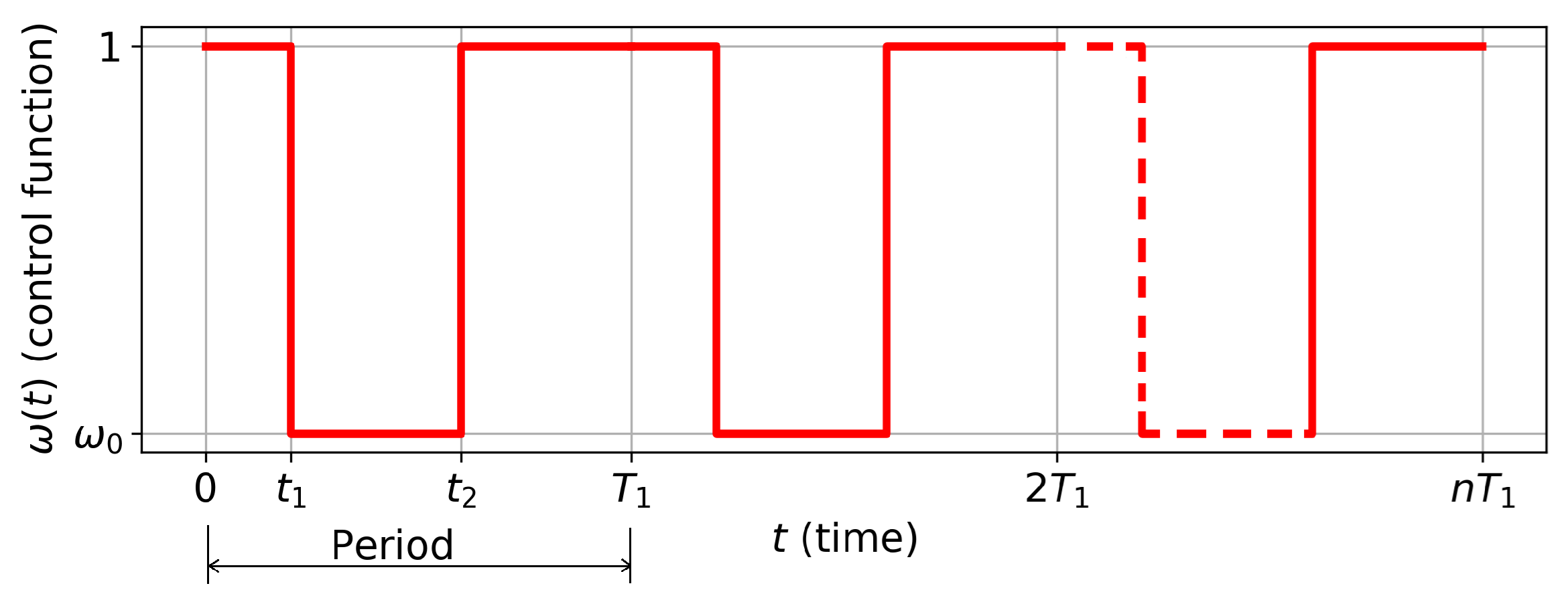
Figure 2.
The trajectory of system (2) on the interval , determined under the periodic control as depicted in Figure 1, satisfies the differential equation and boundary conditions of the system. However, as discussed in the proof of Theorem 1 this trajectory may not be optimal. Here, represent the time points referenced in the statement of Theorem 1.
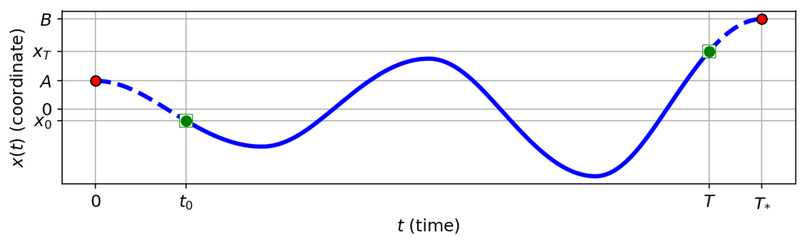
Figure 3.
The reachable set on optimal trajectories of problem (2) for no more than one semi-oscillation is characterized as follows: (a) Damping, (b) Excitation. The blue curve illustrates this elliptical arc: . The red curve illustrates this circular arc: .
Figure 3.
The reachable set on optimal trajectories of problem (2) for no more than one semi-oscillation is characterized as follows: (a) Damping, (b) Excitation. The blue curve illustrates this elliptical arc: . The red curve illustrates this circular arc: .
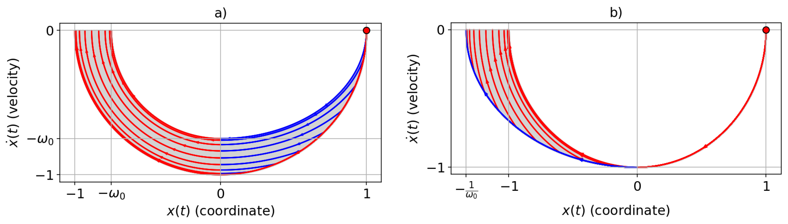
Figure 4.
The reachable set on optimal trajectories of problem (2) for no more than two semi-oscillations is characterized as follows: (a) Damping, (b) Excitation. The blue curve illustrates this elliptical arc: . The red curve illustrates this circular arc: .
Figure 4.
The reachable set on optimal trajectories of problem (2) for no more than two semi-oscillations is characterized as follows: (a) Damping, (b) Excitation. The blue curve illustrates this elliptical arc: . The red curve illustrates this circular arc: .
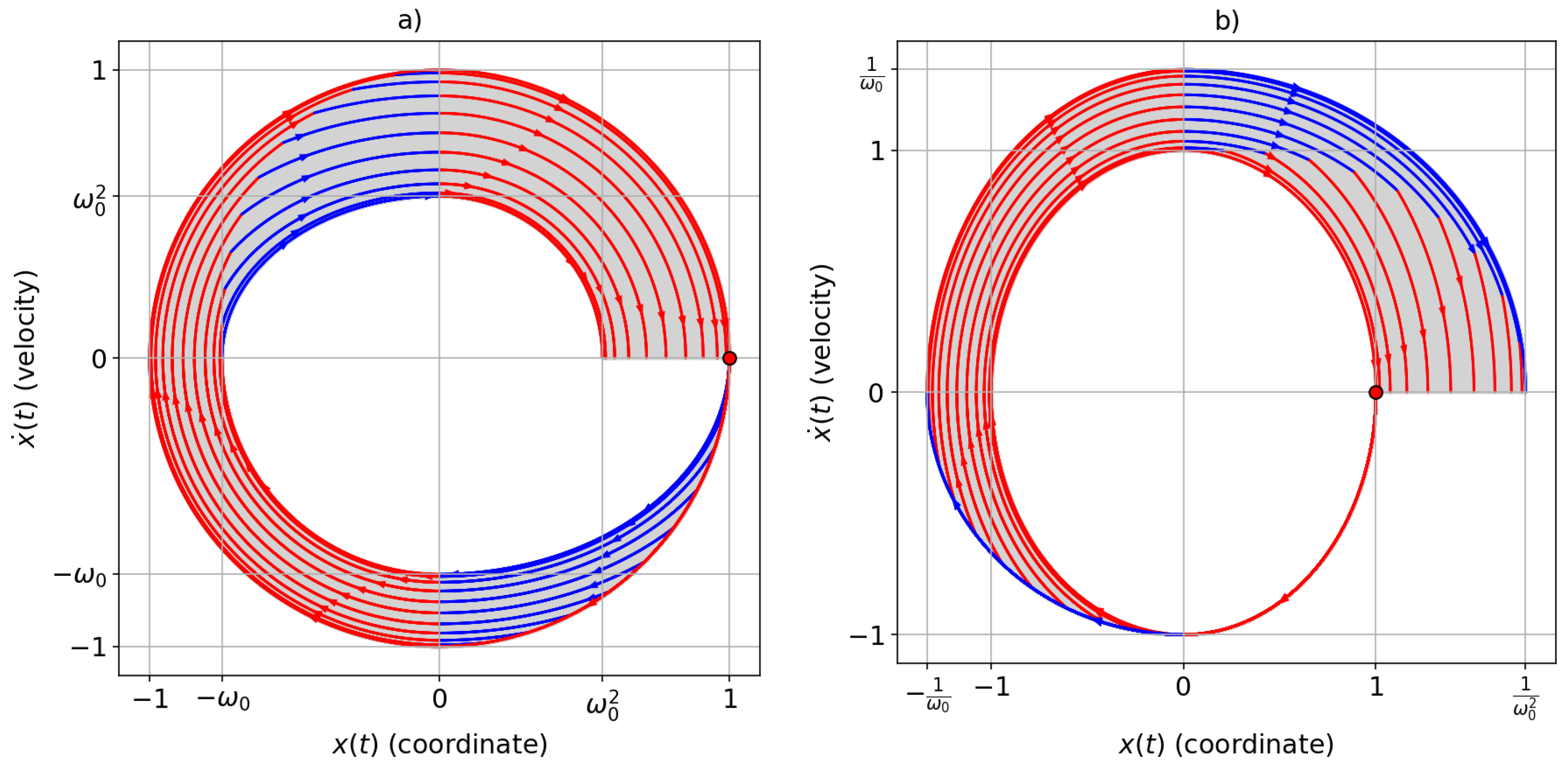
Figure 5.
The reachable set on optimal trajectories of problem (2) for no more than n semi-oscillations (n even). (a) Damping, (b) Excitation.
Figure 5.
The reachable set on optimal trajectories of problem (2) for no more than n semi-oscillations (n even). (a) Damping, (b) Excitation.
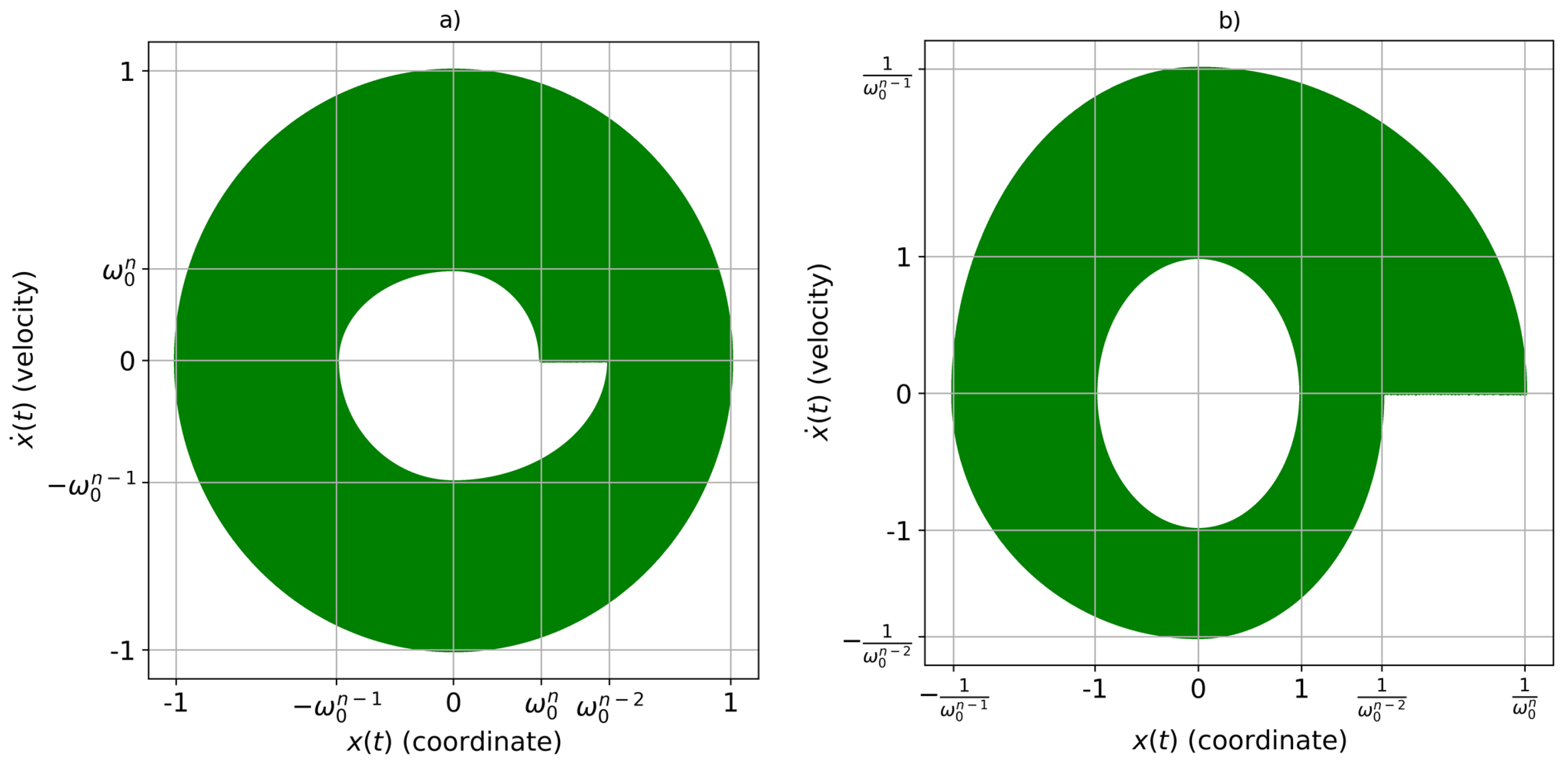
Figure 6.
The trajectory , obtained under the control of the type illustrated in Figure 1, represents a solution to the harmonic oscillator problem with periodic switching between control values and the presumably different solution of the optimal control problem (3).
Figure 6.
The trajectory , obtained under the control of the type illustrated in Figure 1, represents a solution to the harmonic oscillator problem with periodic switching between control values and the presumably different solution of the optimal control problem (3).
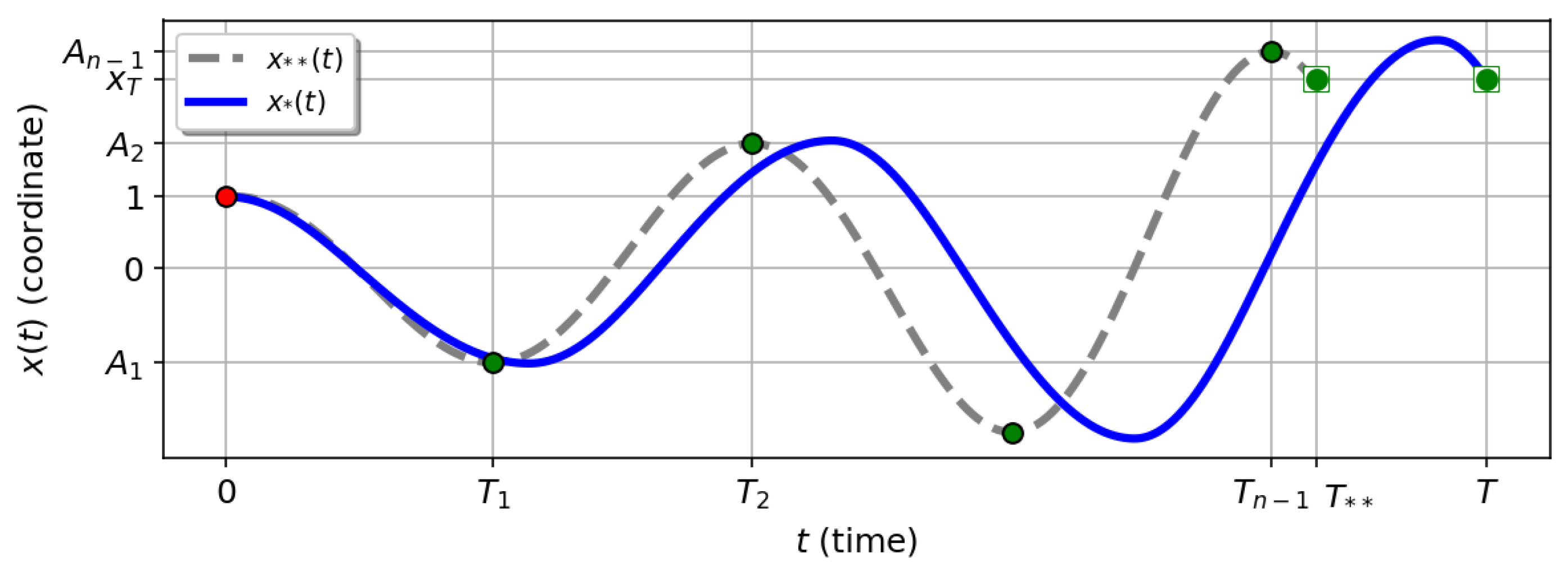
Figure 7.
The optimal trajectory in the optimal control problem (3). (a) Last one incomplete semi-oscillation. (b) Last one complete and one incomplete semi-oscillations.
Figure 7.
The optimal trajectory in the optimal control problem (3). (a) Last one incomplete semi-oscillation. (b) Last one complete and one incomplete semi-oscillations.
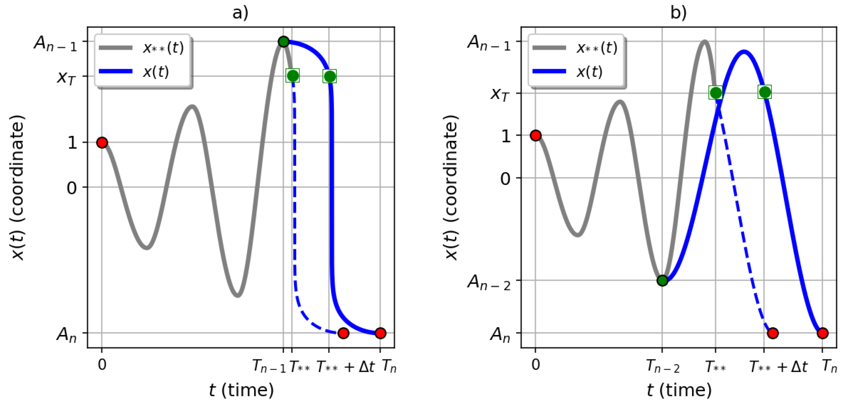
Figure 8.
The reachable set on optimal trajectories of problem (1) for no more than two semi-oscillations is shown for two cases: (a) Damping, (b) Excitation. The blue curve corresponds to an arc of an ellipse described by the equation: . The red curve corresponds to an arc of a circle described by the equation:
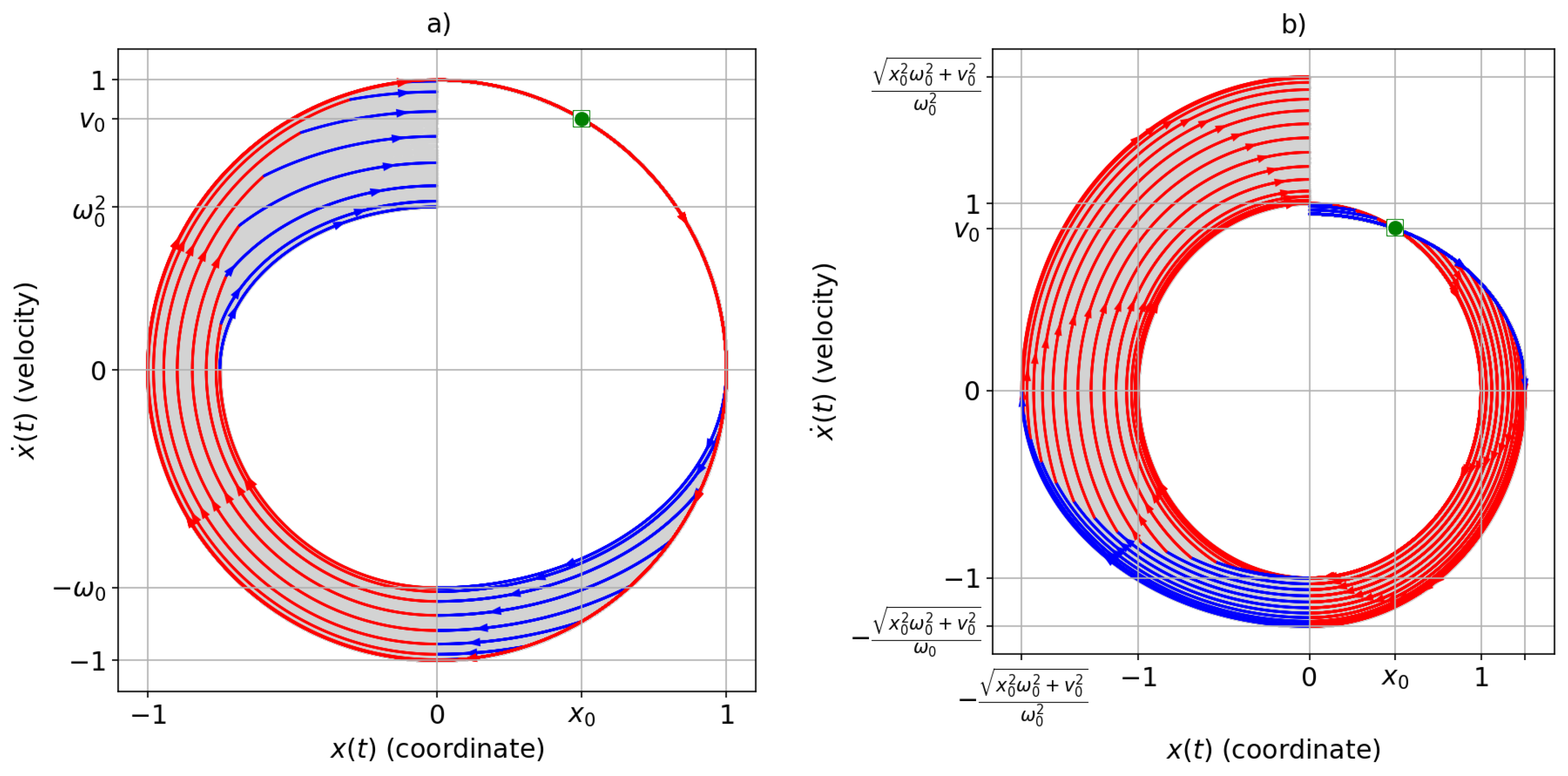
Figure 9.
An example of an optimal trajectory in problem (3) is illustrated by the red curve, which connects the initial point to the endpoint . However, its continuation to the point is not optimal. The reachability set for trajectories requiring at most two semi-oscillations is highlighted in green, indicating the range of states that can be achieved within this constraint.
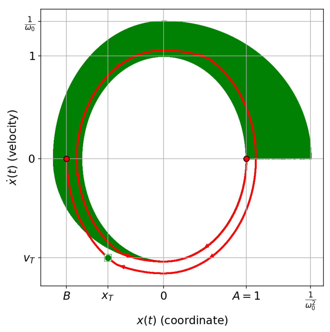
Figure 10.
An example illustrating the dependence of the optimal time on the endpoint is presented. The graph comprises two branches: the outer branch corresponds to oscillations with increasing amplitudes, while the inner branch represents oscillations with decreasing amplitudes. Parameters are set as , , .
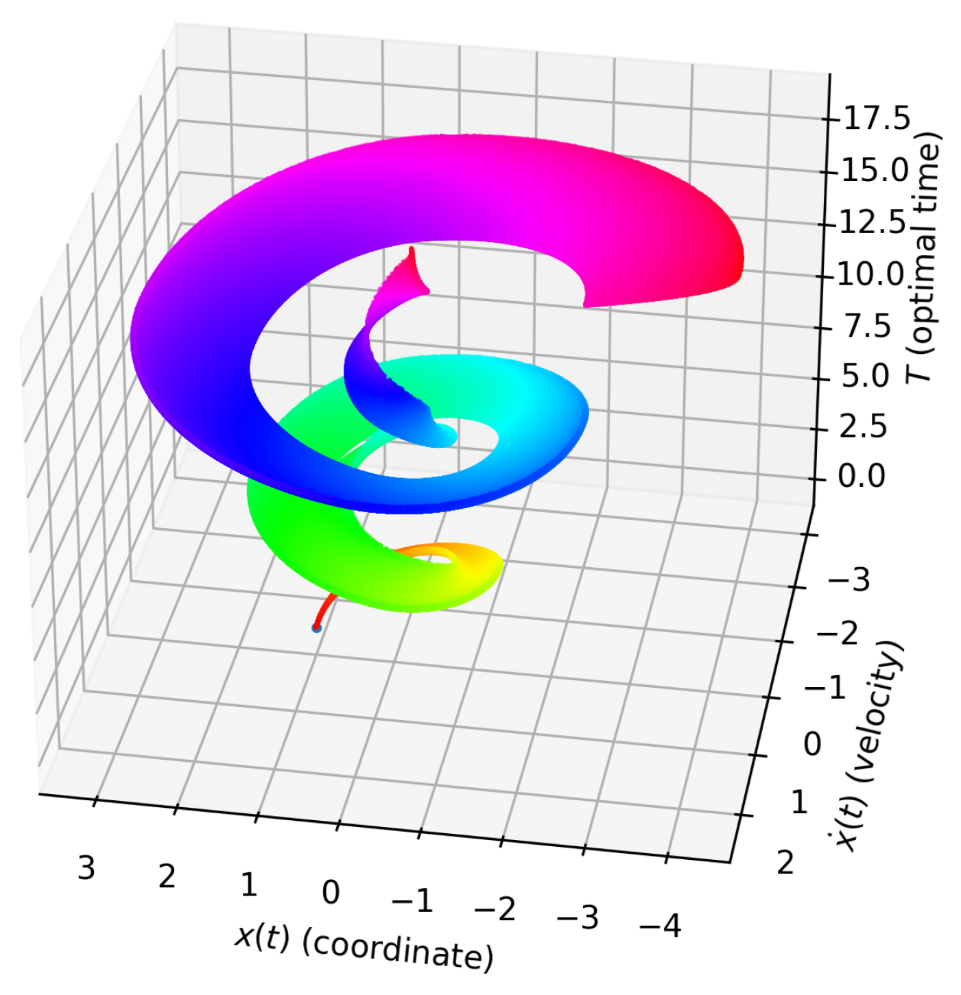
Figure 11.
The task consists of determining the values of the amplitude A and phase shift for the first semi-oscillation. All possible cases of the initial point , where (if , the diagrams will be symmetric with respect to the time axis t), are considered in the case of excitation of oscillations (). For the case of damping oscillations (), refer to Remark 1 (II) for further clarification and details. Similarly, the right endpoint is analyzed to determine the amplitude B and phase shift for the last semi-oscillation.
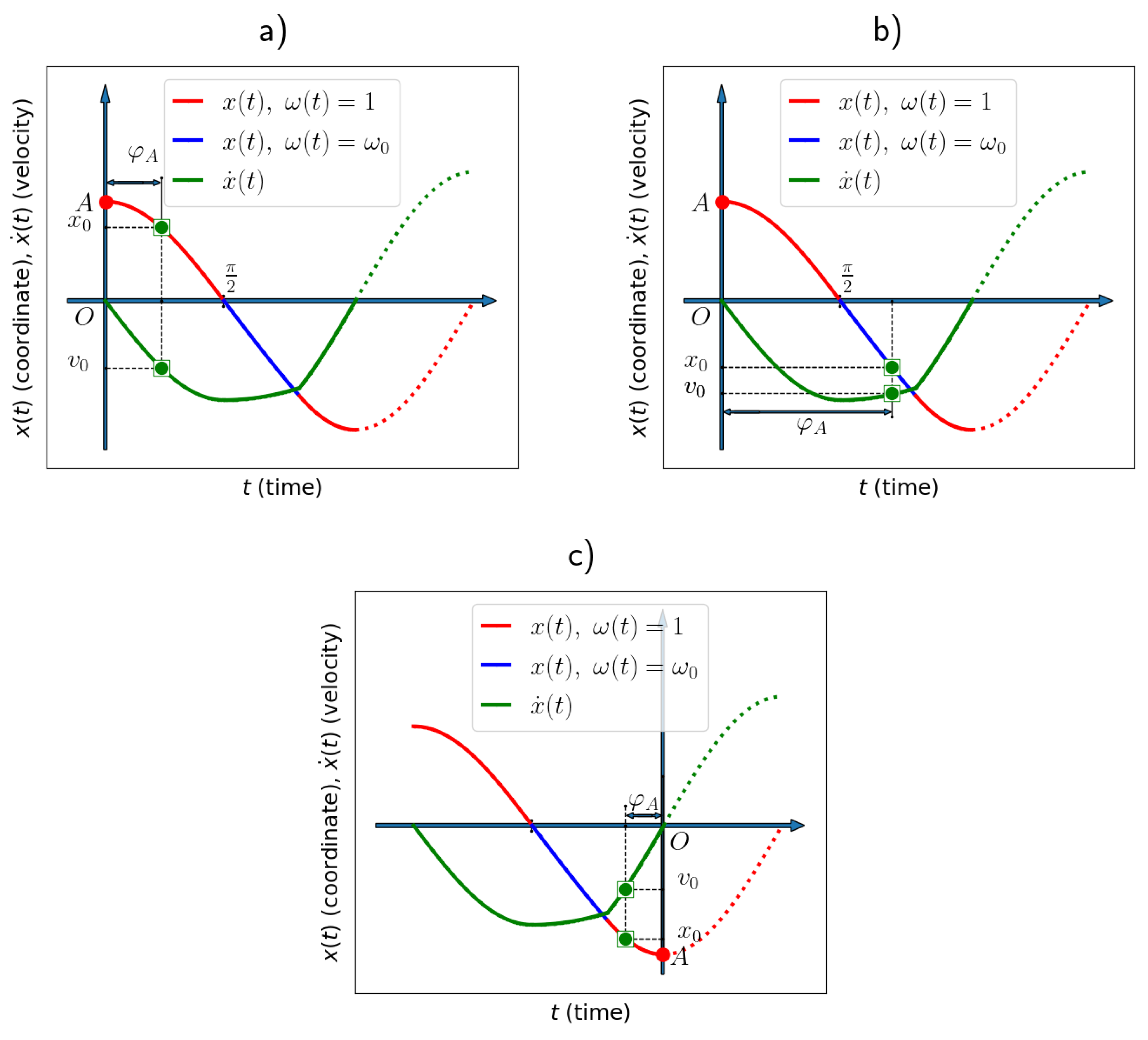
Figure 12.
First step of the algorithm. (a), (b) Trajectory 1 and its phase portrait. (c), (d) Trajectory 2 and its phase portrait. For the given boundary values: Therefore, the trajectory must be modified according to the developed algorithm.
Figure 12.
First step of the algorithm. (a), (b) Trajectory 1 and its phase portrait. (c), (d) Trajectory 2 and its phase portrait. For the given boundary values: Therefore, the trajectory must be modified according to the developed algorithm.
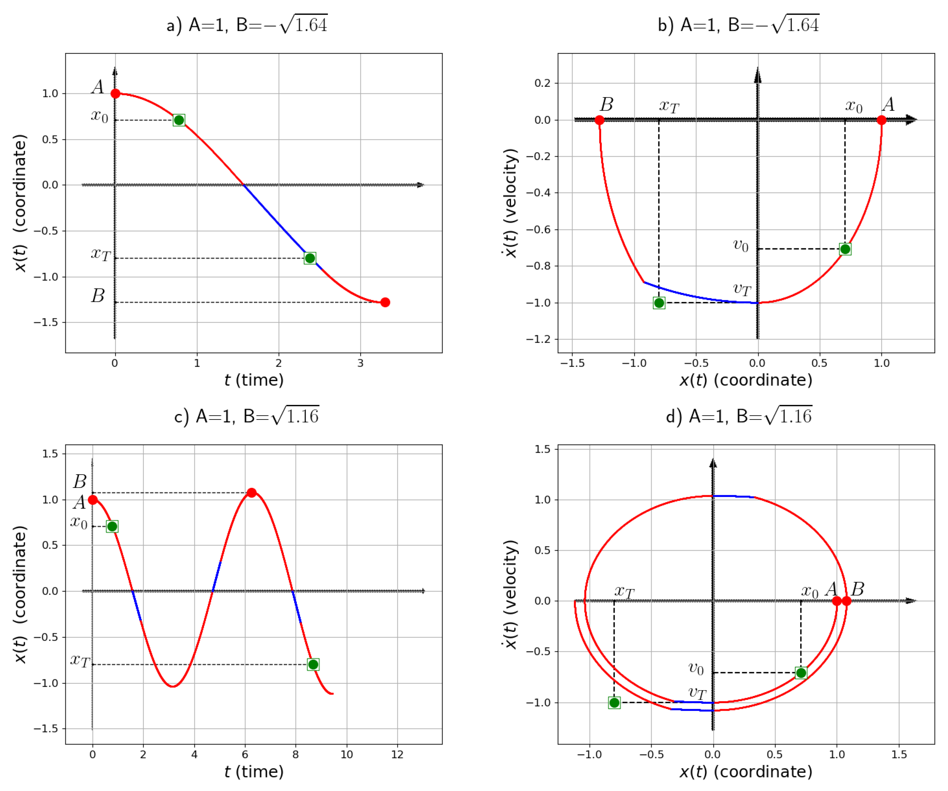
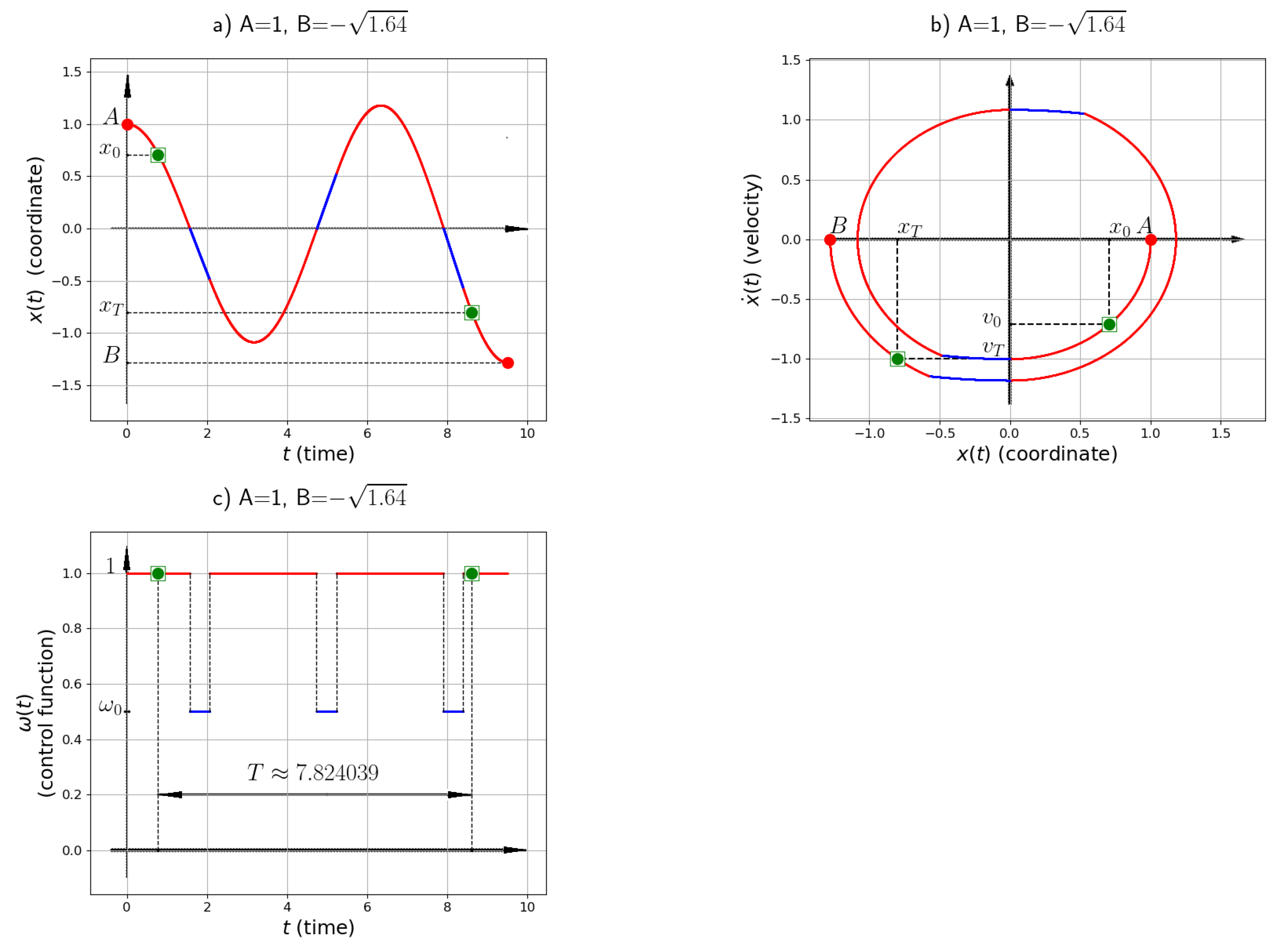
Figure 13.
Solution of the considered example (11). (a) Trajectory. (b) Phase portrait. (c) Control function. The boundary points are located on the optimal trajectory. The duration of the optimal process is
Figure 13.
Solution of the considered example (11). (a) Trajectory. (b) Phase portrait. (c) Control function. The boundary points are located on the optimal trajectory. The duration of the optimal process is
Disclaimer/Publisher’s Note: The statements, opinions and data contained in all publications are solely those of the individual author(s) and contributor(s) and not of MDPI and/or the editor(s). MDPI and/or the editor(s) disclaim responsibility for any injury to people or property resulting from any ideas, methods, instructions or products referred to in the content. |
© 2024 by the authors. Licensee MDPI, Basel, Switzerland. This article is an open access article distributed under the terms and conditions of the Creative Commons Attribution (CC BY) license (http://creativecommons.org/licenses/by/4.0/).
Copyright: This open access article is published under a Creative Commons CC BY 4.0 license, which permit the free download, distribution, and reuse, provided that the author and preprint are cited in any reuse.


