
Submitted:
23 February 2026
Posted:
24 February 2026
You are already at the latest version
Abstract
Background/Objectives: The Human Performance Envelope (HPE) is a multidimen-sional model that represents the range in which an individual operator's performance is acceptable or begins to become dangerous. Although several alternative models have been proposed, HPE currently remains primarily a theoretical concept. The goal of the study was therefore to translate this theoretical concept into practical applications, seeking to characterise and measure how HPE manifests itself in real-world contexts. Methods: Multivariate Autoregressive Models (MVAR) have been used in the analysis of complex systems in which variables are interdependent and mutually influence their dynamics over time. Professional Air Traffic Controllers (ATCOs) were involved in the study and asked to deal with realistic traffic scenarios while their behavioural, subjec-tive and neurophysiological data were collected. Partial Information Decomposition - Least Absolute Shrinkage and Selection Operator (PID – LASSO) model was then em-ployed to estimate the interactions among ATCO’s Human Factors (HFs) and identify the most appropriate characterisation of the HPE. Results: The results showed high and significant correlations among each ATCO’s performance and the corresponding neu-rophysiological – based HPE values. Furthermore, high-performance conditions (Best) were characterized by a significantly higher HPE values and a higher inter-HFs con-nections compared to low-performance (Worst) states. This suggested that a densely interconnected network of HFs is a prerequisite for operational resilience. Conclusions: The study provides the first application of a neurophysiological framework to model the causal interactions between HFs, translating the theoretical HPE into a quantifiable model validated against operator performance.
Keywords:
human performance envelope (HPE)
; neurophysiological
; mental states
; partial information decomposition least absolute shrinkage and selection operator (PID - LASSO)
; human factors (HF)
; air traffic controller (ATCO)
1. Introduction
The relentless evolution of Aviation marked by increasing traffic density, the introduction of trajectory-based operations, and a fundamental shift towards closer human-automation collaboration propels Air Traffic Management (ATM) into an era of unprecedented complexity [1,2,3]. While technology advancements in decision-support tools offer remarkable capabilities, the ultimate guarantor of system safety remains the Air Traffic Controller (ATCO). This reality compels a critical scientific and operational focus on the Human Performance Envelope (HPE). The HPE is a psycho-behavioural concept introduced by Bittner in 1985 [4] with the goal of improving the evaluation of the individual operator. In particular, the HPE is a multid
imensional theoretical model where Human Factors (HFs) define the region in which the operator's performance is acceptable or when the situation becomes dangerous. In other words, depending on the combinations of different HFs, the resulting HPE could move from optimal to degraded [5,6]. For example, when a single HF shows an unacceptable value (e.g., high mental workload), the interaction with all others can compensate it and the overall performance remaining acceptable. In other words, operating within this envelope allows for the graceful management of routine traffic and the adaptive, resilient handling of anomalies. Exceeding the HPE's boundaries precipitates a degradation in performance, a phenomenon characterized by errors of omission (inattention) or commission (misjudgement), loss of situation awareness, and ultimately, a compromise in system safety margins.
This example suggests that HPE cannot simply be modelled as a linear combination of HFs, but it requires a more sophisticated and detailed modelling. Contemporary research has in fact profoundly evolved the understanding of the HPE from a simple, scalar measure of “workload” to a dynamic, multi-layered, and adaptive system [7,8]. The HPE is therefore shaped by a host of intrinsic and extrinsic factors like the expertise, circadian chronotype, trait anxiety, sleep history, and even genetic predispositions [9]. Additionally, cognitive processes are underpinned by a physiological substrate that imposes its own boundaries. These boundaries are elastic and state-dependent. In fact, factors like motivation, time-on-task (fatigue), and perceived risk can expand or contract it momentarily [10]. Furthermore, performance degradation is often non-linear and a system may appear stable until a critical threshold is crossed, leading to a rapid, cliff-edge decline—a phenomenon poorly captured by traditional linear models. It is therefore clear how the concept of HPE is crucial in several high-stakes fields such as Aviation, Space, Transport, Medicine, and Defence. It encompasses the range of conditions under which a human can perform tasks effectively and safely. Understanding the HPE is vital for optimizing human performance, enhancing safety, and designing systems that support human operators.
Over the years, numerous studies aimed at transforming the theoretical HPE model into indicators. One of the most significant attempts is represented by the studies conducted by Alina-Ioana Chira [11]. However, despite the extensive efforts, these studies have been limited to reporting the values of different and single neurometric during various phases of experimentation, without reaching a clear definition of a HPE model, that is where interactions of different HFs have been modelled. A similar approach has been adopted by Victoria Rusu and Gavrila Calefariu [12]. In this case, the focus was on physiological parameters, such as blood pressure and blood oxygen level. Although such studies have represented a significant step forward in the field of research, they did not succeed in providing a complete model for HPE that accurately predicts an individuals’ performance based on the interactions between their own HFs. A more sophisticated and detailed model is necessary. A recent study conducted by Graziani [13] delved into the analysis of HFs within the realm of HPE. Initially, the investigation focused on identifying and evaluating the various HFs involved in the study. The article aimed to explore the potential of Human-Machine Interaction (HMI) as a tool to facilitate recovery and enhance the performance of the subjects under examination. Through careful and targeted analysis, attention gradually shifted from HPE to HMI as the primary focal point for optimizing human performance. Therefore, the article highlighted not only the importance of understanding HFs but also developing targeted strategies for human-machine interaction to maximize human potential and improve overall performance. Another significant contribution in the field of Human Performance Enhancement emerged through the study conducted by Biella [14]. In contrast to previous approaches that had focused on HFs, this work centred on the application of eye tracking as a key analytical tool. The primary goal of the research was to investigate the relationship between subjects' gaze fixation points and their performance in various activities. This innovative approach opened new perspectives in Human Performance Enhancement, providing a detailed and dynamic analysis of visual engagement during specific tasks. Identifying how visual focus directly influences individuals' executive abilities marked a significant step forward in defining Human Performance Enhancement. Another noteworthy study [15] introduced an innovative approach to the analysis of human performance. Within the framework of this study, a device capable of detecting subjects' emotions through heart rate measurement was developed. Through the implementation of this technology, researchers were able to closely examine participants' emotional responses during specific tasks. One of the primary objectives was to assess how emotions influenced individual performance in operational contexts.
These studies clearly demonstrate that, although they have provided fundamental contributions to the development of HPE assessment, they lacked a multidimensional framework capable of translating theories into a concrete method to characterise the dynamic interdependencies between HFs and measure human’s HPE. The aim of the proposed study was therefore to define the HPE not only through theoretical assumptions but also to develop a tangible neurophysiological indicator that can be applied in operational reality. In other words, we aimed at bridging the gap by considering the results of previous studies, empirical observations, and methodological innovation to create a comprehensive and functional framework for HPE measurement. To achieve this goal, ATCOs were asked to perform realistic ATC simulations while their subjective, behavioural and neurophysiological signals were collected. Since ATCOs’ performance is recognised to be impacted by multidimensional aspects such as mental workload, stress, emotions, attentional resources available, attention focus and so on [16], we have employed the Partial Information Decomposition - Least Absolute Shrinkage and Selection Operator (PID – LASSO) model [17,18] to characterize the interactions among different HFs and develop a neurophysiological data – driven HPE model able to describe ATCO’s performance.
We have hence hypothesized that the HPE can be quantified as a dynamic function of causal interactions between HFs, and that a more expansive, densely interconnected HFs network will characterize optimal performance states.
2. Materials and Methods
2.1. Experimental Subjects
Twenty professional ATCOs from the École Nationale de l'Aviation Civile (ENAC, Toulouse, France) have been involved in the study. The group consisted of 17 males and 3 females (mean age: 28 ± 12 years old). Three out of twenty participants reported corrupted data due to technical issues, therefore they were removed from the analyses. The experiments were conducted following the principles outlined in the Declaration of Helsinki of 1975, as revised in 2000. The experiments were approved by the Ethical Committee of ENAC (protocol code 2017/058). Informed consent was obtained from each subject on paper after the study explanation, and all the data were pseudonymized to prevent any association with subject identity in compliance with the current General Data Protection Regulation (GDPR) regulations.
2.2. ATM scenario and experimental protocol
The ATC scenario consisted in three phases where the level of automation changed overtime from high automation (HIGH) to low automation (BASELINE), and finally from low to high automation but with malfunctions (MALFUNCTION). Each phase lasted 8 minutes for a total duration of 24 minutes (Figure 1).
The simulated sector (Figure 2) was an en-route airspace configuration used at ENAC for research and training, therefore no specific familiarisation on the radar platform and airspace had to be done before the experimentation. The traffic used was designed to be a high-density traffic all along the simulation. This means that the average number of aircraft at any time was almost stable and above fifteen. Furthermore, there could be up to three conflicts to solve at the same time. More details about the ATC sector can be found in [19].
2.3. Automation and Malfunction
Automation levels have been defined according to SESAR Level of Automation Taxonomy (LOAT) described in [20]. During the simulation, the BASELINE part was similar to what is provided in current controller’s working positions and used in operations. In the HIGH automation parts of the scenario, specific tools were added to support decision – making, handle conflicts as well as improvements. In particular, the following automations were implemented in the HIGH condition:
- Conflict Solver: it slightly modifies the speed of aircraft in conflict in order to increase the separation. The controller was informed of this action by a clock symbol in their track label (LOAT C & D).
- Situation Awareness monitoring: this tool detects relevant information for ATCOs (i.e. aircraft compliancy to the planned 3D trajectory, communication status) and displays warning and alerts on the track label and a dedicated monitoring window (LOAT B).
- Conflict agenda: this tool shows in an agenda incoming conflicts with detailed information within 15 NM (LOAT B)
- Highlighting of calling station: whenever a pilot calls, the associated aircraft track label is highlighted on the radar screen (LOAT A).
- Reduce visual load: specific information is filtered for non-relevant aircraft to reduce the visual load of the radar screen (LOAT A).
- Adapt STCA alert Design: the short-term conflict alert design is enhanced in order to capture the attention of the air traffic controller (LOAT A).
- Controller Pilot Data Link Communication (CPDLC): CPDLC allows silent communication. It considerably helped to reduce ATCO’s workload linked to radio communication. CPDLC was activated on 60% of the traffic (LOAT D).
During the transition from HIGH automation to BASELINE, all those tools were removed from the controller’s working position interface. During the last phase (MALFUNCTION), the tools were back but inconsistencies appeared in the behaviour of the automation. In particular, the conflict solver flagged aircraft as being managed but the conflict was not solved at all, or the MTCD showed incoherent incoming conflicts. These failures were the same for all ATCOs to avoid confounds in the experimental group.
2.4. Behavioural and Subjective Measure
To collect ATCOs’ behavioural data, a pop-up window appeared on the RADAR interface every minute allowing them to self-assess (Instant Self-Assessment – ISA) and reflect on their own performance regularly. The presence of the pop-up enabled a more detailed and immediate analysis of the level of effectiveness of the actions taken in the last minute. In particular, ATCOs were asked to reply to the following question during the ATC scenario: “are you satisfied about how you are managing the traffic?”. The values given (ATCO ISA) on a scale from 1 to 5 (i.e., 1: very low; 5: very high) and reaction times (ATCO RT) from the window popup onset have been collected. Reaction times provided valuable insights into how quickly and efficiently ATCOs processed the question and provided their ratings. Furthermore, a Subject Matter Expert (SME) closely observed the ATCOs and evaluated their overall performance in terms of safety, efficiency, and strategy. For each phase, SMEs assigned a score (SME ISA), ranging from 1 to 5 (i.e., 1: very low; 5: very high), allowing for a comprehensive and articulate assessment of overall performance. The integration of these perspectives provided us with a comprehensive overview of controller performance, enabling to evaluate not only operational effectiveness but also subjective perception and critical analysis from industry experts. The Performance Index was therefore defined by the following formula:
In other words, the ratings provided by the ATCO (ATCO ISA) were normalised by those of SMEs (SME ISA) to make them more reliable. These coefficients were successively used to weight ATCO’s reaction times (ATCO RT) and define a performance index able to consider ATCO’s traffic management dynamics (i.e. safety, efficiency, and strategy) and their reaction times. The logic behind this approach was to establish a direct relationship between a positive self-assessment and subjective evaluation, indicative of good performance, and a low reaction time, which was considered an indicator of efficiency and readiness in performing the required actions.
2.5. Neurophysiological Data Recording and Analysis
Controllers’ brain activity, Electroencephalographic (EEG) data, was recorded using the BEmicro (EBNeuro, Italy) digital monitoring system with a sampling frequency of 256 Hz. Sixteen Ag/AgCl gel-based electrodes were positioned over ATCOs’ scalp according to the 10 - 20 International System [21]. Specifically, electrodes were placed at Fpz, F3, Fz, F4, AF3, AFz, AF4, C3, C4, P3, Pz, P4, POz, O1, Oz, and O2 referenced to both the mastoids and grounded to the Cz. Prior to data collection, electrode impedance was verified to be below 10 kΩ to ensure adequate signal quality [22]. Before analysis, the EEG data underwent a pre-processing phase aimed at identifying and correcting physiological and non-physiological artifacts unrelated to cerebral activity of interest (e.g., ocular movements, muscle activity, body motion). Signals were band-pass filtered between 2–30 Hz using a 5th-order Butterworth filter. Eye-blink artifacts were detected and corrected in real time using the o-CLEAN method [23,24]. Additional artifacts, including those from muscular activity and movements, were identified and removed using ad-hoc algorithms based on the EEGLAB toolbox [25]. The data reported an average of 20% of artifact epochs. MVAR algorithms require sufficient data samples per condition to estimate a stable model. When a class has too few samples, the system of equations becomes underdetermined or ill-conditioned. In fact, parameter estimation yields high-variance coefficients, model order selection criteria become unreliable, and cross-spectral density matrices may be singular, making connectivity metrics meaningless [26,27]. Oversampling approach can augment the minority class before MVAR model estimation ensuring that each class contributes adequately to parameter estimation [28,29]. In this regard, the Synthetic Minority Over-sampling Technique (SMOTE) is able to generate new synthetic samples that lie along the manifold of the minority class, producing plausible, diverse new observations rather than exact copies [28]. The mathematical justification for this approach is rooted in the assumption that the space between two instances of the same class is also likely to belong to that class [30]. Consequently, in correspondence of the artifact epochs, we inserted synthetic values by using the SMOTE with the aim to obtain reliable MVAR model and keep temporal alignment among the different HFs [28]. From the artifact-free EEG data, the Global Field Power (GFP) was computed within the Theta, Alpha, Beta and Gamma bands which were individually defined based on each participant’s IAF [31]. The IAF was determined from a 60-second baseline recording acquired with participants’ eyes closed, a condition that reliably enhances the alpha peak. Subsequently, EEG GFP features were extracted for each 1-second epoch using a Hanning window of matching length, yielding to a frequency resolution of 1 Hz. On the basis of the original definition of the HPE proposed by Bittner[32], we targeted five HFs to both avoid redundant information and provide the accurate neurophysiological characterisation of the HPE: Mental Workload, Attention, Stress, Vigilance and Effort [5,6,13]. The corresponding Neurometrics were derived in accordance with previous works [33,34,35,36,37,38,39,40,41,42,43]:
Mental Workload = Theta Frontal / Alpha High Parietal
Attention = - AlphaFrontal
Vigilance = - Beta Frontal
Stress = Beta High Parietal
Effort = Theta Frontal
Each neurometric consisted in a vector of 3 (phases) * 8 (duration of each phase in minutes) * 60 (resolution of a second) = 1440 samples. As the PID – LASSO requires that its inputs must have normal (gaussian) distributions, the neurometrics were normalised using the z-score transformation [44].
2.6. PID – LASSO Model
The neurophysiological – based model of the HPE started from its original definition [4]. The goal was therefore to identify a model able to estimate the effective connectivity among the considered HFs, that is the causal, directed influence one HF exerts over others. In particular, the model had to estimate HFs interactions by determining (i) the types of information gleaned from multiple variables collectively, (ii) the information exclusive to specific variables but not others, and (iii) the information accessible only when examining certain variables in conjunction [45]. Additionally, we needed to take into account the characteristics of the dataset in terms of data length (i.e. 24 minutes) and number of variables to be considered simultaneously (i.e. 5 HFs). Accurately disentangling these directed interactions from high-dimensional, noisy, and mixed-source EEG data represents a challenge. In response to this challenge, the Partial Information Decomposition (PID) with the rigorous regularization power of the Least Absolute Shrinkage and Selection Operator (LASSO) framework turned out to be the most appropriate methodological approach [46,47]. In fact, traditional linear methods for assessing directed connectivity, such as Granger Causality (GC) and its multivariate extensions (e.g. multivariate Granger causality - MVGC) operate on a principle of temporal precedence and predictability: if the past of time series X improves the prediction of the future of time series Y beyond the past of Y itself, a directed influence from X to Y is inferred [48]. Also, GC – based models are inherently bivariate or low-order multivariate struggling to differentiate between a true direct connection and an indirect interaction mediated by a third or more variables (e.g. 5 HFs). On the contrary, PID moves beyond simple mutual information to decompose the total information that a set of "source" variables provides about a "target" variable into distinct components: unique information (provided by one source alone), redundant information (provided redundantly by multiple sources), and synergistic information (only available when considering sources jointly) [49]. Additionally, estimating the requisite information-theoretic quantities from finite, noisy EEG data requires modelling the joint probability distributions of multiple time series. This is where the integration with the LASSO regression became pivotal. LASSO is a regularized regression technique that performs variable selection by imposing an L1-norm penalty on the regression coefficients, driving many of them to exactly zero. This results in a sparse solution, effectively identifying a parsimonious subset of predictors that are most relevant for forecasting the target signal [50]. The core innovation lies in using LASSO not merely as a filter, but as an integral part of the connectivity and information decomposition process. In other words, we used the LASSO-regularized estimator to automatically identify the sparse set of most influential past states from all possible HFs for predicting each HF's future. The resulting sparse MVAR model inherently represented a directed functional network, filtering out weak or spurious connections (i.e. interactions). Second, this sparse connectivity structure was used to define the relevant sets of "source" variables for each HF. Finally, the PID decomposed the information flow along each identified connection into a unique and synergistic components [17,18]. This sequential regularization mitigated dimensionality and yielded a more stable, interpretable estimates of causal interactions.
2.7. PID-LASSO Order Model Selection
The selection of optimal model order for multivariate autoregressive (MVAR) models typically employs information-theoretic criteria, predominantly the Akaike Information Criterion (AIC) [51] and the Bayesian Information Criterion (BIC) [52], which balance model goodness-of-fit against parametric complexity. The AIC, formulated to minimize prediction error, tends to favor more complex models and is asymptotically efficient but may not converge to a unique optimal order, particularly in high-dimensional systems. In essence, AIC seeks the model that is expected to perform best on new, unseen data drawn from the same distribution. Its formula, AIC = 2k - 2 log(L), balances the negative log-likelihood (-2 log(L)), which decreases with better fit, against a penalty term (2k) that increases linearly with the number of parameters k. A key property of AIC is that it is asymptotically efficient: as sample size n grows, the order model (p) selected by AIC will achieve the smallest possible prediction error. However, even with infinite data, AIC may not converge to the simplest "true" model if it exists, as it does not penalize complexity harshly enough to guarantee the selection of the correct finite-dimensional model when one truly exists. Conversely, the BIC, BIC = k log(n) -2 log(L), incorporates a stronger penalty term proportional to (k log(n)), where n is the sample size and k is the number of parameters. This logarithmic dependence on n is crucial as for any sample size larger than 7, the BIC penalty per parameter is more severe than AIC's. This grants BIC its defining property: it is asymptotically consistent. In other words, given a set of candidate order models that includes the true finite-dimensional model, as the sample size n tends to infinity, the probability that BIC selects this true model converges to 1. This makes BIC preferable in scenarios where the primary goal is model identification which was the objective of our study [53,54].
2.8. Human Performance Envelope (HPE) Characterisation
Graph indexes are capable of objectively describe the network derived from the application of the PID – LASSO model on the HFs data series [55,56,57,58]. In other words, graph indexes synthesize the complex dynamics of HFs relationships over time, providing a concise yet comprehensive representation of the variation and structure of connections between HFs. The goal was therefore to accurately and fully capture the interactions between different HFs allowing for a deeper understanding of underlying processes and their implications for behaviour and cognitive functions. Among the existing graph indexes, we considered the PageRank, Graph’s Density Index, and Shannon Entropy for the HPE model characterisation. The reason behind this selection is described here below:
- PageRank (PR) is used to evaluate the importance of each node based on the number of incoming relationships and the rank of the related source nodes [58]. PR effectively returns the probability distribution representing the likelihood of visiting a particular node (i.e. HF) through a random traversal of the graph. Essentially, the PR assesses the importance of each HF based on its connectivity with other high-ranking nodes (i.e. HFs) in the graph. This means that nodes with a large number of inbound links from high-ranking nodes tend to have a higher PR score. The resulting probability distribution allows for understanding which nodes are more central or influential in the overall structure of the network. The PR of the i-th node (e.g. HF) was calculated by the following formula:
- Graph’s Density (D) is a measure that indicates how many connections between nodes exist compared to how many connections between nodes are possible [59]. For an undirected simple graph with N vertices and E edges, the density D is calculated as:

In other words, the density of a graph provides an indication of the strength of connections within the network. It represents the ratio between the actual number of connections present in the graph and the maximum number of connections that could exist considering all possible links between the nodes in the network. As a consequence, it can assume values within the range [0 ÷ 1]. A high D suggests a densely interconnected network, where most nodes are connected to each other. Conversely, a low D indicates a more dispersed or fragmented network, with few connections between nodes. Measuring the D of a graph allows for understanding the cohesion and complexity of relationships within the network, providing valuable information about its structure and its resilience to variations and external events.
- Shannon’s Entropy is essentially a measure of the uncertainty or information contained in a random data source. More precisely, it is the average amount of information produced by a stochastic data source [60,61]. When discussing "information," it refers to how significant or surprising a new value in a process is. If Shannon entropy is high, it indicates that there are many different possibilities or a lot of variation in the data, so each new value obtained provides a considerable amount of additional information. Conversely, if entropy is low, it implies there are few possibilities or little variation, thus each new value does not contribute significantly to the information. The model used in our study was based on the Conditional Transfer Entropy (cTE), which is a measure of the amount of information that one HF (i.e. node) can transfer to another HF, considering the conditional relationships between their states and other HFs. On the other hand, Shannon Entropy is a measure of the amount of uncertainty or disorder in an information system. In short, while Shannon’s Entropy assesses the uncertainty or disorder in a single HF, cTE evaluates the amount of information that can be transmitted among the HFs, considering the conditional relationships between them [62]. The cTE of the i-the node which transfers information to the j-th node considering the presence (i.e. conditioning) of the k-th node was calculated by the following formula:
where σ(r) and σ(r) are variances of the prediction error in the full (u) ensemble of nodes (i.e. i, j and k) and in the restricted (r) obtained from the full by removing the i-th node (i.e. j and k). Due to the normalization of the series, cTE ranged within 0 and 1 (where cTE > 0), indicating perfect and poor prediction respectively.
We noticed that the influence of a given HF on the overall system is proportional to its centrality (PR) and the cohesion of its local network (D), but inversely proportional to the uncertainty or disorder in its information dynamics (cTE). In other words, the increase in a HF's number of incoming links with other HFs was closely correlated with the overall participant’s performance improvement. Conversely, as the cTE of an HF increased, a decrease in the participant’s performance was noticed. These findings led us to the hypothesis that the characterisation and contribution to HPE of each HF ( could be modelled by a coefficient derived from the product of PR and its D, all divided by the corresponding cTE as reported in the following formula:
The resultant HF* values for the five HFs defined points in a 5-dimensional performance space ranging from 0 to 1. For visualization and scalar quantification, we projected them onto a 2D space, where the area enclosed by the vertices HF* provided a single and integrative metric of the HPE at time t (Figure 3). This follows the geometric intuition that a larger Area of the polygon (an irregular pentagon) represented a greater interaction across all HFs, that is a higher HPE [4,6,13]. The measure of participants’ HPE was therefore obtained by measuring the Area of such an irregular pentagon by using the Gauss's Area Formula (or Shoelace Formula) as described in [63]:
A graphical representation of the HPE model characterisation is reported in Figure 3. By analysing the area of the polygon, which reflects HFs interaction and intersection, a more complete and accurate view of the participant’s performance could be obtained.
3. Results
3.1. Behavioural Results
The Controllers’ Performance Index has been analysed across the three experimental conditions. Although a slightly decreased has been noted in the BASELINE condition with respect the ones where the automation was enabled, the repeated measure ANOVA did not report any statistical effects (F = 2.02; p = 0.15; ƞ2 = 0.096).
3.2. ATCO ISA Results
The repeated measure ANOVA on the ISA scores provided by the Controllers during the execution of the ATC scenario did not report any statistical differences (F = 0.67; p = 0.52; ƞ2 = 0.04). In particular, the Controllers exhibited almost the same perception under the different experimental conditions.
3.3. SME ISA Results
Similarly to the Controllers, also the statistics on the ISA scores provided by the SMEs along the ATC scenario did not report any significant effects (F = 2.4, p = 0.1, ƞ2 = 0.11).
3.4. PID-LASSO Model Order Selection
To identify the best model order, we computed both AIC and BIC across the range of order values n = [1 ÷ 20] to identify the order that minimized the respective criterion. When the orders of AIC and BIC differed, we selected the BIC as it penalizes complexity more strongly, thus it is generally more reliable for real data model identification [64,65]. This is also advantageous for avoiding overfitting in noisy data, producing a more stable and interpretable model, and is often considered safer when the goal is inference about the existence of connections (e.g., in network analysis), as it controls false positives more conservatively in the large-sample limit. Table 1 reports the order model n selected for each participant.
These model orders were then used to estimate the corresponding HPE models for each participant which were considered in the analyses.
3.5. HPE Results
HPE values of participants have been averaged within each of the three experimental conditions (HIGH, BASELINE and MALFUNCTION). The repeated measure ANOVA on these HPEs did not return any significant effects (F = 1.15, p = 0.33, ƞ2 = 0.067) along the ATC scenario.
3.6. HPE corresponding to high and low performance
Based on the original HPE definition, participants’ HPE should have changed with their performance levels. In this regard, we identified the temporal moments t corresponding to participants’ maximum (Best) and minimum (Worst) performance values. In particular, 42% of worst performance occurred during HIGH, 42% during BASE and 16% in MALFUNCTION. The best performance occurred for 50% of cases in HIGH, 22% in MALFUNCTION, and 28% in BASE. Coherently with these moments, we computed the corresponding HPE values and then performed statistics on these distributions. Error! Reference source not found. shows the average HPE during the best (HPE max, green colour) and worst (HPE min, red colour) performance.
Figure 4.
Representation of the average HPE during the best (HPE max, green colour) and worst (HPE min, red colour) performance.
Figure 4.
Representation of the average HPE during the best (HPE max, green colour) and worst (HPE min, red colour) performance.
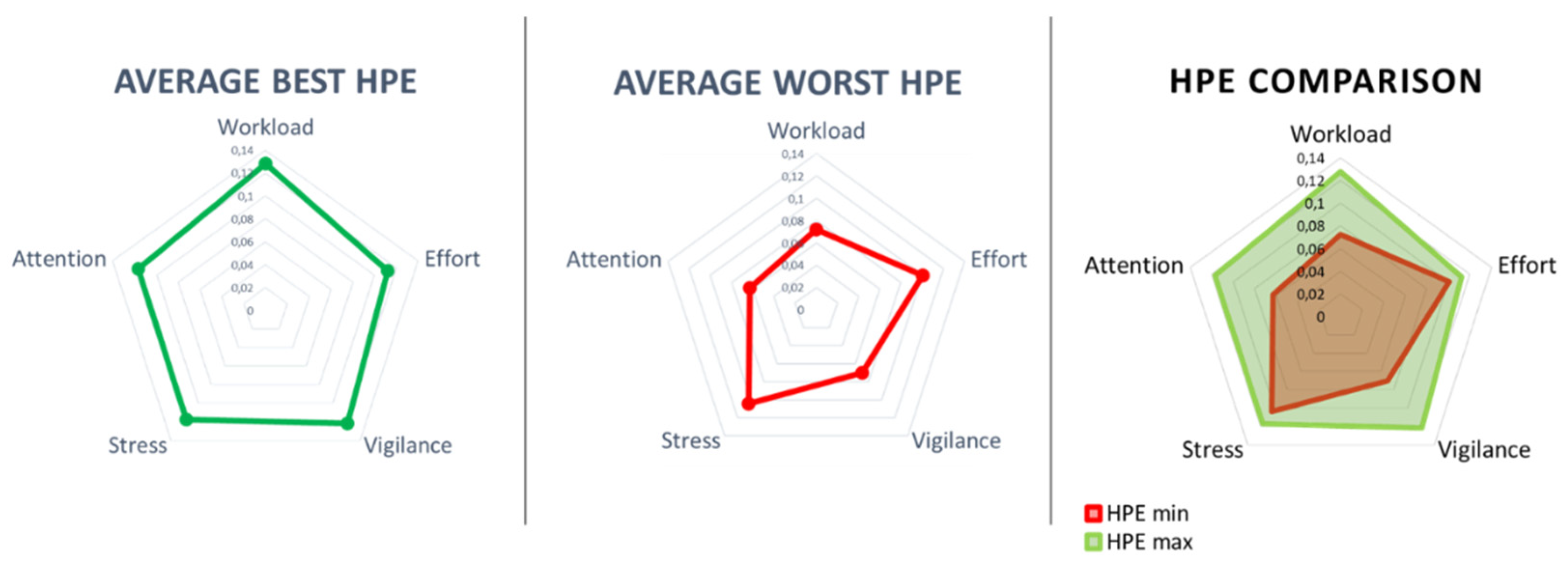
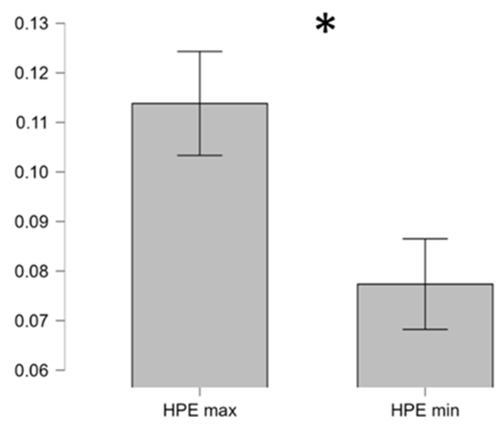
In particular, it is possible to note how the area of the corresponding polygon during the worst performance (HPE min = 0.07) was lower than the one during the best performance (HPE max = 0.11). As reported in the HPE model definition [4,6,13], a bigger area of the HPE suggests a more effective performance, indicating that the controllers operated successfully across a wider range of cognitive conditions. Conversely, a smaller area of the HPE suggests a more limited performance, indicating that the controllers may have encountered greater difficulty. The paired two-tail t-test on average HPE values between the Best and Worst condition showed a significant difference (t = 3.06, p = 0.009, Cohen’s d = 0.82) suggesting HPEs changed significantly when the controllers performed better (Error! Reference source not found.).
Figure 5.
The two-tail paired t-test on the average HPE showed a significant difference between the best (HPE max, green polygon) and worst (HPE min, red polygon) performance condition.
Figure 5.
The two-tail paired t-test on the average HPE showed a significant difference between the best (HPE max, green polygon) and worst (HPE min, red polygon) performance condition.
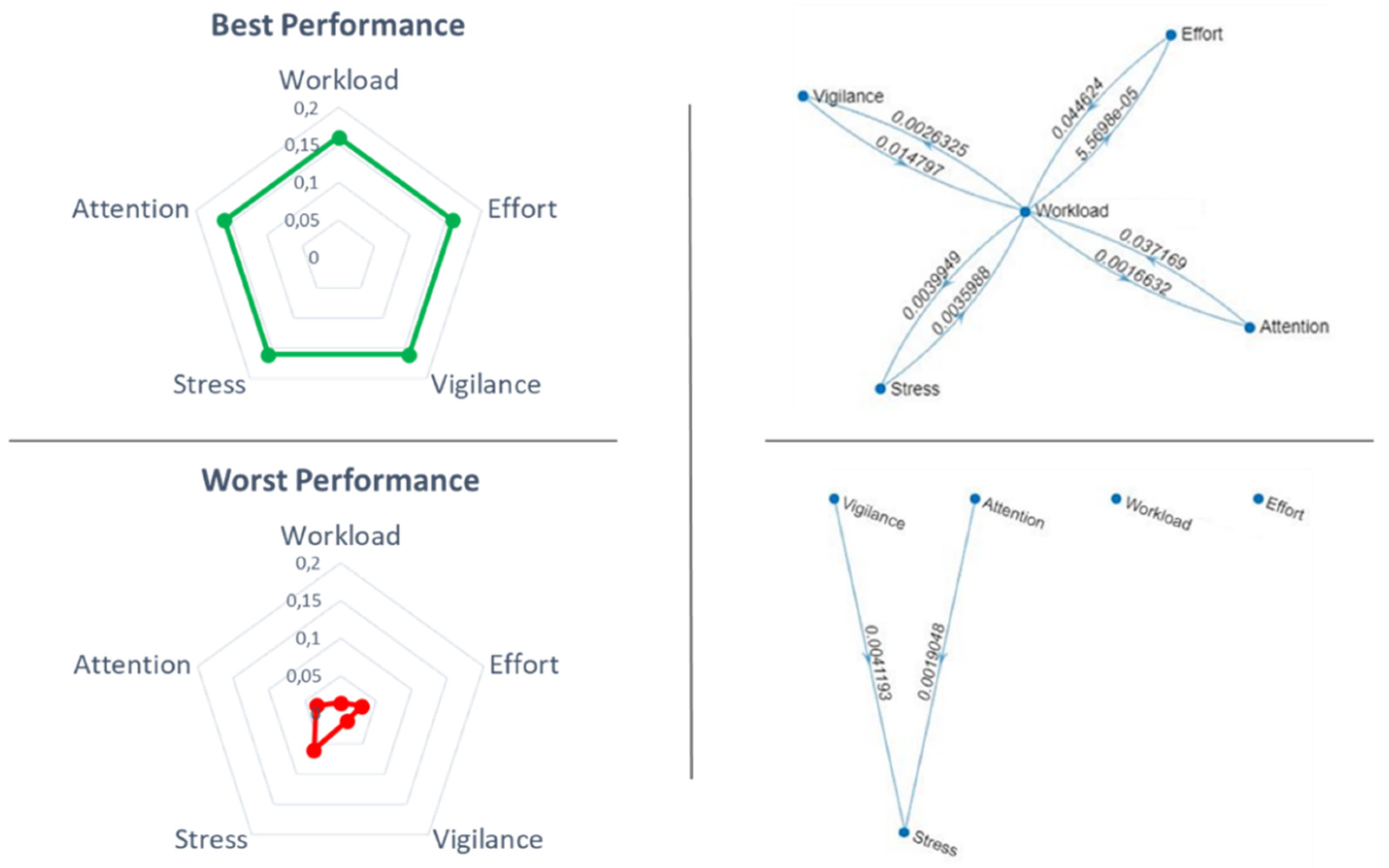
It was also very interesting to investigate what happened in terms of HFs interactions (i.e. number of links) under these conditions. It turned out that when the participant’s performance was the best, all the considered HFs (i.e. Mental Workload, Effort, Attention, Stress and Vigilance) were densely interconnected (top panel right side of Error! Reference source not found.). On the contrary, when the controllers’ performance assumed the worst value, most of links among the considered HFs drastically reduced (bottom panel right side of Error! Reference source not found.). In the left side of Error! Reference source not found. are represented the HPE during, respectively, the best and worst performance of a representative participant.
Figure 6.
Number of connections among HFs of a representative participant in correspondence of the best (green polygon) and worst (red polygon) performance condition.
Figure 6.
Number of connections among HFs of a representative participant in correspondence of the best (green polygon) and worst (red polygon) performance condition.
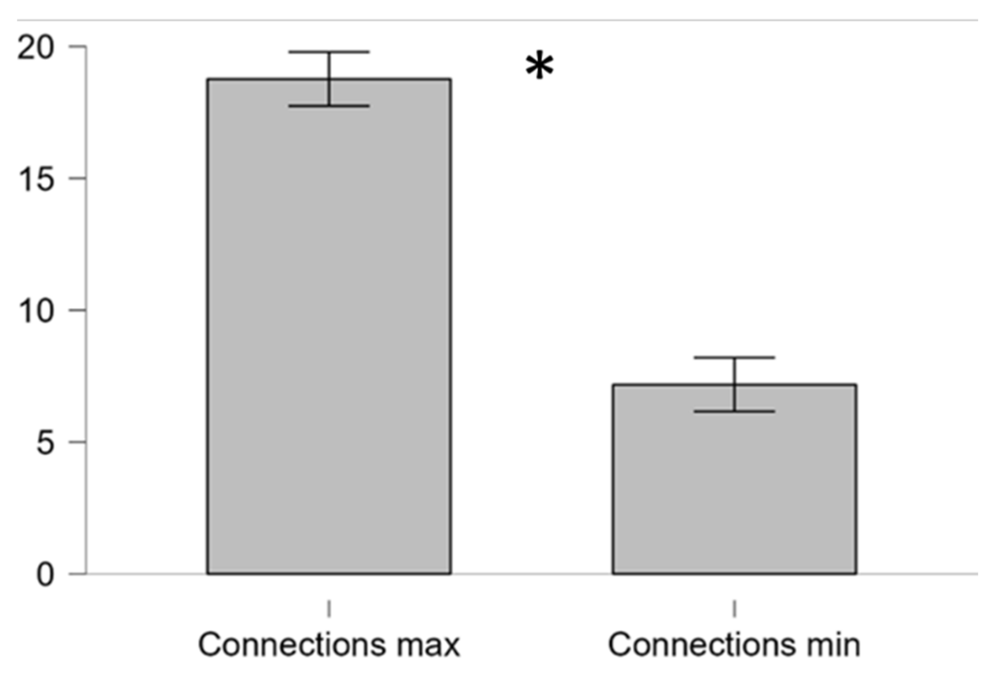
In particular, the paired two-tail t-test on the average number of connections among HFs related to the best and worst performance condition showed a significant difference (t = 8.02, p < 0.001, Cohen’s d = 1.95) suggesting that interactions and dynamics among HFs, hence the HPE, changed significantly when the controllers performed better (Error! Reference source not found.).
Figure 7.
The two-tail paired t-test on the average number of connections related to the best (Connection max) and worst (Connection min) performance showed a significant difference.
Figure 7.
The two-tail paired t-test on the average number of connections related to the best (Connection max) and worst (Connection min) performance showed a significant difference.
3.7. Correlation between HPE and Performance Index
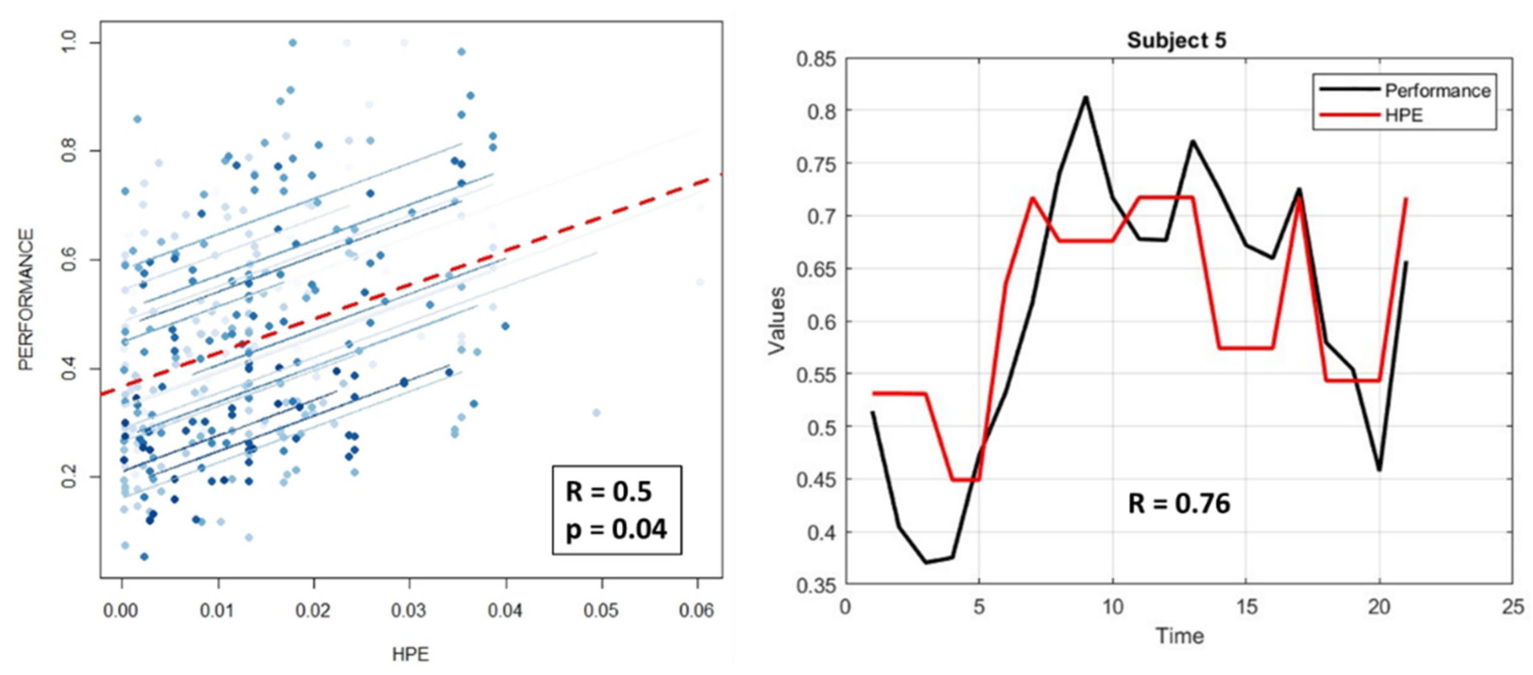
To better evaluate the proposed neurophysiological - based HPE model, we investigated the relationship between individual performance and the corresponding HPE values over time. In this regard, repeated measure correlation (rmcorr) analysis [66] was performed on these parameters to obtain a validation at both single-participant and experimental group level. For each participant, HPE values were averaged within each minute to have vectors of same lengths as the performance ones. Error! Reference source not found. shows the results of the rmcorr analysis reporting a positive overall correlation coefficient R = 0.5 and a significant statistics with p = 0.04 (left panel). The correlation between the HPE and Performance of a representative participant (S5) is reported in the right panel of Error! Reference source not found.. It is possible to note the high and positive correlation (R = 0.76) between the two parameters.
Figure 8.
The repeated measure correlation (rmcorr) analysis on participants’ performance and the corresponding HPE values over time returned a positive (R = 0.5) and significant (p = 0.04) correlation (left panel). In the right panel it is possible to note the high and positive correlation (R = 0.76) for a representative participant.
4. Discussion
The objective of the work was to develop a neurophysiological – based model of the Human Performance Envelope (HPE). The HFs considered for the HPE characterisation were the Mental Workload, Vigilance, Stress, Effort and Attention. These HFs allowed for a comprehensive understanding of the participants’ cognitive and emotional states. However, the focus was not solely on HFs intrinsic values to define HPE, but rather on exploring their mutual influence and interaction. The objective was therefore to find a model that, considering the combination and interaction among the different HFs, could accurately describe participants’ performance. In doing so, we had to understand how these HFs integrated and influenced each other. In this regard, the PID-LASSO model was adopted. From the networks returned by the PID – LASSO we identified three graph indexes able to describe the interaction between HFs: PageRank (PR), Graph Density (D) and Conditional Transfer Entropy (cTE). The PR and D take into account the degree and number of relationships of each HF with the others. When the cTE increases, indicating more disorder and complications in the subgraph, performance decreases. Consequently, the contribution of each HF to the participant’s HPE was calculated using (10). Such values defined a polygon whose area turned out to be the proposed HPE measure through (11).
The analyses on behavioural, subjective and neurophysiological data across the three experimental phases (HIGH, BASELINE, MALFUNCTION) did not provide with any significant difference. This result could be explained by the fact that Air Traffic Controllers always strive to perform at their best regardless of the ongoing situation.
However, based on the original HPE definition, significant differences were found in correspondence of condition of highest (best) and lowest (worst) performance. In particular, both the area of polygons charactering the average HPE (Error! Reference source not found.) and average number of connections (i.e. links) among HFs (Error! Reference source not found.) under such conditions reported significant differences. In other words, operational resilience and performance were underpinned by a densely interconnected operators’ HFs, supporting the causal and multivariate model of the HPE.
Furthermore, to assess the potential relationship between the proposed neurophysiological HPE characterisation model and human performance, repeated measures correlation analysis was performed on HPEs and the corresponding participant performance over time. The result returned a positive (R = 0.5) and significant (p = 0.04) evidence of how high HPE values corresponded to high performance, and vice – versa.
Although the results were very promising and provided with a significant and promising framework on the relationships between a multivariate combination of neurophysiological indicators and participants’ performance, we have to highlight some limitations of the study and actions for the next study. In particular:
- Controller performance assessments were derived from subjective ratings (SME and ATCO) therefore they might not fully represent their performance.
- The sample size consisted of twenty participants, therefore enlarged group is needed for further validate the result. Additionally, validations in other contexts (e.g. automotive, surgery) will be considered.
- Other MVAR models (e.g. modification of the backward-in-time selection – mBTS, and Partial Multivariate Information-based Non-uniform Embedding - PMIME) will be considered to take into account non-linear connections among HFs.
- More HFs (e.g. Engagement, Mental Fatigue) and neurophysiological parameters like Heart Rate, Skin Conductance, and Eye Tracking will be considered into the HPE model definition for a more comprehensive and accurate understanding of dynamics for HPE characterisation.
5. Conclusions
Understanding the HPE is essential for optimizing performance and safety in high-stakes environments. By considering behavioural and physiological factors, and leveraging advanced monitoring technologies, we can ensure that individuals operate within their performance limits, thereby reducing the risk of errors and accidents. A model of the HPE can guide the development of advanced competency-based training, pushing trainees to safely explore their boundaries in simulation contexts. In fact, by making the invisible boundaries of human performance visible, measurable and central to design, we could provide with a more efficient and capacious but, above all, more resilient and human-centric training framework, ensuring that humans remain the keystone of safety in the increasingly complex working contexts.
This work did not simply mark the end point in the research on HPE, but rather represents a significant step towards achieving something concrete. The goal is to provide a tangible contribution that can serve as inspiration for future studies and lead to the necessary improvements to optimize HPE to its full potential.
Additionally, developing integrated models that combine physiological, behavioural, psychological, and environmental data will provide a more holistic understanding of the HPE. These models can predict performance outcomes under various conditions and help in designing better support and adaptive systems [67]. In fact, adaptive systems can respond to real-time monitoring data and adjust task demands or provide support accordingly to help keeping individuals performance within their HPE. These systems will enhance performance and safety in high-stakes environments [68].
Author Contributions
Conceptualization, G.B. S.B. V.A. P.T. F.D. J.P.I. and G.G.; methodology, G.B. K.L. G.D.F. P.A. V.R. A.G. R.C. and A.R.; software, G.B. G.D.F. P.A. V.R. A.G. R.C. A.R. J.P.I. and G.G.; validation, G.B. G.D.F. S.B. V.A. P.T. F.D. J.P.I. and G.G.; formal analysis, G.B. K.L. R.C. A.R. V.A. and P.T.; investigation, G.B. S.B. F.D. J.P.I. and G.G.; resources, G.B. S.B. J.P.I. and F.B..; data curation, G.B. S.B. and J.P.I.; writing—original draft preparation, G.B. S.B. J.P.I. and G.G.; writing—review and editing, K.L. G.D.F. P.A. V.R. A.G. R.C. A.R. V.A. P.T. F.D. and F.B.; visualization, G.B. K.L. J.P.I. and G.G.; supervision, G.B. S.B. F.D. and F.B.; project administration, S.B. J.P.I and F.B.; funding acquisition, S.B. J.P.I and F.B. All authors have read and agreed to the published version of the manuscript.
Funding
This work was co-funded by the European Commission by H2020 projects “STRESS: Wearable device to decode human mind by neurometrics for a new concept of smart interaction with the surrounding environment” (GA n. 950998).
Institutional Review Board Statement
The study was conducted in accordance with the Declaration of Helsinki, and approved on the 5th of December 2017 (protocol code 2017/058) by the Institutional Review Board (or Ethics Committee) of the École Nationale de l'Aviation Civile (ENAC).
Informed Consent Statement
Informed consent was obtained from all subjects involved in the study. Written informed consent has been obtained from the participants to publish this paper and of any potentially identifiable images or data included in this article.
Data Availability Statement
The datasets presented in this article are not readily available because raw data might be shared upon reasonable request to the corresponding author. Requests to access the datasets should be directed to gianluca.borghini@uniroma1.it.
Acknowledgments
The authors would like to acknowledge the “CODA” (GA: 101114765) and “TRUSTY” project provided by the HORIZON -SESAR EU program, the “SPACE IT UP” project funded by the Italian Space Agency, ASI, and the Ministry of University and Research, MUR (contract n. 2024-5-E.0 - CUP n. I53D24000060005). Individual grants must be also acknowledged, especially the ones by the Italian Ministry of University and Research through the projects SIMU2DRIVE (CUP: B53C24009580001), funded to Prof. Gianluca Di Flumeri through the Fondo Italiano per la Scienza (FIS 2023) Starting Grant; “REMES-Remote tool for emotional states evaluation” provided to Vincenzo Ronca, and “HF AUXAviation: Advanced tool for Human Factors evaluation for the AUXiliary systems assessment in Aviation” provided by Sapienza University of Rome to Vincenzo Ronca, “TCI: Neurophysiological Framework for Predicting Team Dynamics in High-Responsibility Operational Environments -Team-Computer Interface” provided by the Sapienza University of Rome to Pietro Aricò (CUP B83C24007070005) and for financial support under the National Institute for Insurance against Accidents at Work, through the “NeuroUX5.0” project, within the program BRIC, grant number CUP B83C24006240005.
Conflicts of Interest
The authors declare no conflicts of interest.
References
- J. Lundberg, M. Arvola, and K. L. Palmerius, “Human Autonomy in Future Drone Traffic: Joint Human–AI Control in Temporal Cognitive Work,” Front. Artif. Intell., vol. 4, p. 704082, Jul. 2021. [CrossRef]
- B. Kirwan, “Human Factors Requirements for Human-AI Teaming in Aviation,” Future Transportation 2025, Vol. 5, vol. 5, no. 2, Apr. 2025. [CrossRef]
- F. T. Durso and C. A. Manning, “Air Traffic Control,” Reviews of Human Factors and Ergonomics, vol. 36, no. SUPP, pp. 10–12, 2008. [CrossRef]
- A. C. Bittner, M. M. Harbeson, R. S. Kennedy, and N. C. Lundy, “Assessing the Human Performance Envelope: A Brief Guide,” SAE Technical Papers, Oct. 1985. [CrossRef]
- T. Edwards, “HUMAN PERFORMANCE IN AIR TRAFFIC CONTROL,” 2013.
- S. Silvagni, L. Napoletano, I. Graziani, P. Le Blaye, and L. Rognin, “Concept for Human Performance Envelope,” Future Sky Safety, 2015.
- A.R. Pritchett, “Aviation Automation: General Perspectives and Specific Guidance for the Design of Modes and Alerts,” Reviews of Human Factors and Ergonomics, vol. 5, no. 1, pp. 82–113, Jun. 2009. [CrossRef]
- S. D. Ae and E. Hollnagel, “Human factors and folk models,” 2004. [CrossRef]
- R. Hockey, “The psychology of fatigue: Work, effort and control,” The Psychology of Fatigue: Work, Effort and Control, pp. 1–272, Jan. 2011. [CrossRef]
- P. A. Hancock and J. S. Warm, “A dynamic model of stress and sustained attention,” Hum. Factors, vol. 31, no. 5, pp. 519–537, 1989. [CrossRef]
- A.I. Chira, A. Dumitrescu, C. S. Moisoiu, and C. A. Tanase, “Human Performance Envelope Model Study Using Pilot’s Measured Parameters,” INCAS Bulletin, vol. 12, no. 4, pp. 49–61, 2020. [CrossRef]
- V. Rusu and G. Calefariu, “Mathematical-heuristic modelling for human performance envelope,” Human Systems Management, vol. 42, no. 2, pp. 233–246, 2023. [CrossRef]
- Graziani et al., “Development of the Human Performance Envelope Concept for Cockpit HMI Design,” 2016.
- M. Biella, “Human Performance Envelope: Overview of the Project and Technical Results,” 2018, Accessed: Feb. 09, 2026. [Online]. Available: https://emojiterra.com/de/landung-eines-flugzeugs/.
- A.Dumitrescu, R. Craciunescu, and A. Vulpe, “Evaluation of Human Performance in Driving Scenarios,” International Symposium on Wireless Personal Multimedia Communications, WPMC, vol. 2022-October, pp. 369–374, 2022. [CrossRef]
- “Human Performance in Air Traffic Management Safety A White Paper,” 2010.
- L. Novelli, P. Wollstadt, P. Mediano, M. Wibral, and J. T. Lizier, “Large-scale directed network inference with multivariate transfer entropy and hierarchical statistical testing,” Network Neuroscience, vol. 3, no. 3, pp. 827–847, Jul. 2019. [CrossRef]
- T. Lizier, N. Bertschinger, J. Jost, and M. Wibral, “Information Decomposition of Target Effects from Multi-Source Interactions: Perspectives on Previous, Current and Future Work,” Entropy 2018, Vol. 20, vol. 20, no. 4, Apr. 2018. [CrossRef]
- G. Borghini et al., “EEG-Based Cognitive Control Behaviour Assessment: An Ecological study with Professional Air Traffic Controllers,” Sci. Rep., vol. 7, no. 1, 2017. [CrossRef]
- Save and B. Feuerberg, “Designing Human-Automation Interaction: a new level of Automation Taxonomy,” 2012.
- V. Jurcak, D. Tsuzuki, and I. Dan, “10/20, 10/10, and 10/5 systems revisited: Their validity as relative head-surface-based positioning systems,” Neuroimage, vol. 34, no. 4, pp. 1600–1611, Feb. 2007. [CrossRef]
- N. Sciaraffa et al., “Evaluation of a New Lightweight EEG Technology for Translational Applications of Passive Brain-Computer Interfaces,” Front. Hum. Neurosci., vol. 16, p. 458, Jul. 2022. [CrossRef]
- V. Ronca et al., “o-CLEAN: a novel multi-stage algorithm for the ocular artifacts’ correction from EEG data in out-of-the-lab applications,” J. Neural Eng., vol. 21, no. 5, Oct. 2024. [CrossRef]
- G. Di Flumeri, P. Arico, G. Borghini, A. Colosimo, and F. Babiloni, “A new regression-based method for the eye blinks artifacts correction in the EEG signal, without using any EOG channel,” Annu. Int. Conf. IEEE Eng. Med. Biol. Soc., vol. 2016, pp. 3187–3190, Oct. 2016. [CrossRef]
- A.Delorme and S. Makeig, “EEGLAB: an open source toolbox for analysis of single-trial EEG dynamics including independent component analysis,” J. Neurosci. Methods, vol. 134, no. 1, pp. 9–21, Mar. 2004. [CrossRef]
- A. Baccalá and K. Sameshima, “Partial directed coherence: a new concept in neural structure determination,” Biol. Cybern., vol. 84, no. 6, pp. 463–474, 2001. [CrossRef]
- Kamiński, M. Ding, W. A. Truccolo, and S. L. Bressler, “Evaluating causal relations in neural systems: granger causality, directed transfer function and statistical assessment of significance,” Biol. Cybern., vol. 85, no. 2, pp. 145–157, 2001. [CrossRef]
- V. Chawla, K. W. Bowyer, L. O. Hall, and W. P. Kegelmeyer, “SMOTE: Synthetic Minority Over-sampling Technique,” Journal of Artificial Intelligence Research, vol. 16, pp. 321–357, Jun. 2002. [CrossRef]
- G. Haixiang, L. Yijing, J. Shang, G. Mingyun, H. Yuanyue, and G. Bing, “Learning from class-imbalanced data: Review of methods and applications,” Expert Syst. Appl., vol. 73, pp. 220–239, May 2017,. [CrossRef]
- H. He and E. A. Garcia, “Learning from imbalanced data,” IEEE Trans. Knowl. Data Eng., vol. 21, no. 9, pp. 1263–1284, Sep. 2009. [CrossRef]
- W. Klimesch, “EEG alpha and theta oscillations reflect cognitive and memory performance: a review and analysis,” Brain Res. Rev., vol. 29, no. 2–3, pp. 169–195, Apr. 1999. [CrossRef]
- A.C. Bittner, M. M. Harbeson, R. S. Kennedy, and N. C. Lundy, “Assessing the human performance envelope: A brief guide,” in SAE Technical Papers, SAE International, 1985. [CrossRef]
- G. Borghini, L. Astolfi, G. Vecchiato, D. Mattia, and F. Babiloni, “Measuring neurophysiological signals in aircraft pilots and car drivers for the assessment of mental workload, fatigue and drowsiness,” Neurosci. Biobehav. Rev., vol. 44, pp. 58–75, 2014. [CrossRef]
- V. Ronca et al., “Neurophysiological Assessment of An Innovative Maritime Safety System in Terms of Ship Operators’ Mental Workload, Stress, and Attention in the Full Mission Bridge Simulator,” Brain Sciences 2023, Vol. 13, Page 1319, vol. 13, no. 9, p. 1319, Sep. 2023. [CrossRef]
- G. Borghini et al., “Real-time Pilot Crew’s Mental Workload and Arousal Assessment During Simulated Flights for Training Evaluation: a Case Study,” Annu. Int. Conf. IEEE Eng. Med. Biol. Soc., vol. 2022, pp. 3568–3571, 2022. [CrossRef]
- Aricò et al., “Adaptive Automation Triggered by EEG-Based Mental Workload Index: A Passive Brain-Computer Interface Application in Realistic Air Traffic Control Environment,” Front. Hum. Neurosci., vol. 10, no. OCT2016, p. 539, Oct. 2016. [CrossRef]
- N. Sciaraffa et al., “Validation of a Light EEG-Based Measure for Real-Time Stress Monitoring during Realistic Driving,” Brain Sciences 2022, Vol. 12, Page 304, vol. 12, no. 3, p. 304, Feb. 2022. [CrossRef]
- M. Sebastiani, G. Di Flumeri, P. Aricò, N. Sciaraffa, F. Babiloni, and G. Borghini, “Neurophysiological Vigilance Characterisation and Assessment: Laboratory and Realistic Validations Involving Professional Air Traffic Controllers,” Brain Sciences 2020, Vol. 10, Page 48, vol. 10, no. 1, p. 48, Jan. 2020. [CrossRef]
- G. Di Flumeri et al., “Brain–Computer Interface-Based Adaptive Automation to Prevent Out-Of-The-Loop Phenomenon in Air Traffic Controllers Dealing With Highly Automated Systems,” Front. Hum. Neurosci., vol. 13, p. 469230, Sep. 2019. [CrossRef]
- N. Sciaraffa, G. Borghini, G. Di Flumeri, F. Cincotti, F. Babiloni, and P. Aricò, “Joint Analysis of Eye Blinks and Brain Activity to Investigate Attentional Demand during a Visual Search Task,” Brain Sci., vol. 11, no. 5, May 2021. [CrossRef]
- N. Sciaraffa et al., “Evaluation of a New Lightweight EEG Technology for Translational Applications of Passive Brain-Computer Interfaces,” Front. Hum. Neurosci., vol. 16, p. 458, Jul. 2022. [CrossRef]
- Simonetti et al., “Neurophysiological Evaluation of Students’ Experience during Remote and Face-to-Face Lessons: A Case Study at Driving School,” Brain Sciences 2023, Vol. 13, Page 95, vol. 13, no. 1, p. 95, Jan. 2023. [CrossRef]
- G. Borghini et al., “Air Force Pilot Expertise Assessment during Unusual Attitude Recovery Flight,” Safety 2022, Vol. 8, Page 38, vol. 8, no. 2, p. 38, May 2022. [CrossRef]
- A.Jain, K. Nandakumar, and A. Ross, “Score normalization in multimodal biometric systems,” Pattern Recognit., vol. 38, no. 12, pp. 2270–2285, Dec. 2005. [CrossRef]
- J. Gutknecht, M. Wibral, and A. Makkeh, “Bits and pieces: understanding information decomposition from part-whole relationships and formal logic,” Proc. Math. Phys. Eng. Sci., vol. 477, no. 2251, Jul. 2021. [CrossRef]
- S. Haufe, V. V. Nikulin, K. R. Müller, and G. Nolte, “A critical assessment of connectivity measures for EEG data: A simulation study,” Neuroimage, vol. 64, no. 1, pp. 120–133, Jan. 2013. [CrossRef]
- A. Valdes-Sosa, A. Roebroeck, J. Daunizeau, and K. Friston, “Effective connectivity: Influence, causality and biophysical modeling,” Neuroimage, vol. 58, no. 2, pp. 339–361, Sep. 2011. [CrossRef]
- X. Wen, G. Rangarajan, and M. Ding, “Multivariate Granger causality: an estimation framework based on factorization of the spectral density matrix,” Philos. Trans. A Math. Phys. Eng. Sci., vol. 371, no. 1997, p. 20110610, Aug. 2013. [CrossRef]
- L. Williams and R. D. Beer, “Nonnegative Decomposition of Multivariate Information,” Apr. 2010, Accessed: Feb. 10, 2026. [Online]. Available: http://arxiv.org/abs/1004.2515.
- Tibshirani, “Regression Shrinkage and Selection Via the Lasso,” J. R. Stat. Soc. Series B Stat. Methodol., vol. 58, no. 1, pp. 267–288, Jan. 1996. [CrossRef]
- H. Akaike, “Information Theory and an Extension of the Maximum Likelihood Principle,” Biogeochemistry, vol. 1998, pp. 199–213, 1998. [CrossRef]
- G. Schwarz, “Estimating the Dimension of a Model,” The Annals of Statistics, vol. 6, no. 2, pp. 461–464, Mar. 1978. [CrossRef]
- Ding, V. Tarokh, and Y. Yang, “Model Selection Techniques-An Overview,” IEEE Signal Process. Mag., 2018. [CrossRef]
- Claeskens Gerda and Hjort Nils Lid, “Model Selection and Model Averaging,” Cambridge University Press, Cambridge, vol. 5, 2008, Accessed: Feb. 10, 2026. [Online]. Available: www.cambridge.org.
- F. D. V. Fallani et al., “A graph-theoretical approach in brain functional networks. Possible implications in EEG studies,” Nonlinear Biomedical Physics 2010 4:1, vol. 4, no. 1, pp. S8-, Jun. 2010. [CrossRef]
- Kuntzelman and V. Miskovic, “Reliability of graph metrics derived from resting-state human EEG,” Psychophysiology, vol. 54, no. 1, pp. 51–61, Jan. 2017. [CrossRef]
- Y. Lou et al., “Graph theory-based analysis of functional connectivity changes in brain networks underlying cognitive fatigue: An EEG study,” PLoS One, vol. 20, no. 8, p. e0329212, Aug. 2025. [CrossRef]
- A.H. Ghaderi, B. R. Baltaretu, M. N. Andevari, V. Bharmauria, and F. Balci, “Synchrony and Complexity in State-Related EEG Networks: An Application of Spectral Graph Theory,” Neural Comput., vol. 32, no. 12, pp. 2422–2454, Dec. 2020. [CrossRef]
- Dattola, N. Mammone, F. C. Morabito, D. Rosaci, G. M. L. Sarné, and F. La Foresta, “Testing Graph Robustness Indexes for EEG Analysis in Alzheimer’s Disease Diagnosis,” Electronics 2021, Vol. 10, vol. 10, no. 12, Jun. 2021. [CrossRef]
- Y. Karaca and M. Moonis, “Shannon entropy-based complexity quantification of nonlinear stochastic process: diagnostic and predictive spatiotemporal uncertainty of multiple sclerosis subgroups,” Multi-Chaos, Fractal and Multi-Fractional Artificial Intelligence of Different Complex Systems, pp. 231–245, Jan. 2022, Accessed: Feb. 10, 2026. [Online]. Available: https://www.sciencedirect.com/science/chapter/edited-volume/abs/pii/B9780323900324000183.
- A.A. Torres-García, O. Mendoza-Montoya, M. Molinas, J. M. Antelis, L. A. Moctezuma, and T. Hernández-Del-Toro, “Pre-processing and feature extraction,” Biosignal Processing and Classification Using Computational Learning and Intelligence: Principles, Algorithms, and Applications, pp. 59–91, Jan. 2021. [CrossRef]
- V. Bari et al., “Cerebrovascular and cardiovascular variability interactions investigated through conditional joint transfer entropy in subjects prone to postural syncope,” Physiol. Meas., vol. 38, no. 5, pp. 976–991, Apr. 2017. [CrossRef]
- J. Gechlik, S. High School-Saratoga, and C. H. Sedrakyan, “Gauss’s Area Formula for Irregular Shapes,” Ohio Journal of School Mathematics, vol. 97, no. 1, Jul. 2024. [CrossRef]
- I. Vrieze, “Model selection and psychological theory: a discussion of the differences between the Akaike information criterion (AIC) and the Bayesian information criterion (BIC),” Psychol. Methods, vol. 17, no. 2, pp. 228–243, Jun. 2012. [CrossRef]
- A.D. R. McQuarrie and C.-L. Tsai, “Regression and Time Series Model Selection,” Regression and Time Series Model Selection, May 1998. [CrossRef]
- J. Z. Bakdash and L. R. Marusich, “Repeated measures correlation,” Front. Psychol., vol. 8, no. MAR, p. 456, Apr. 2017. [CrossRef]
- G. Matthews, J. S. Warm, L. E. Reinerman, L. K. Langheim, D. J. Saxby, and https://gmu.academia.edu/GeraldMatthews, “Task Engagement, Attention, and Executive Control,” The Springer Series on Human Exceptionality, pp. 205–230, 2010. [CrossRef]
- R. Parasuraman and C. D. Wickens, “Humans: still vital after all these years of automation,” Hum. Factors, vol. 50, no. 3, pp. 511–520, Jun. 2008. [CrossRef]
Figure 1.
The ATC scenario consisted of three phases during which automation intervention changed: high automation (HIGH), low automation (BASELINE), and finally from low to high automation but with malfunctions (MALFUNCTION). Each phase lasted 8 minutes for a total scenario of 24 minutes.
Figure 1.
The ATC scenario consisted of three phases during which automation intervention changed: high automation (HIGH), low automation (BASELINE), and finally from low to high automation but with malfunctions (MALFUNCTION). Each phase lasted 8 minutes for a total scenario of 24 minutes.
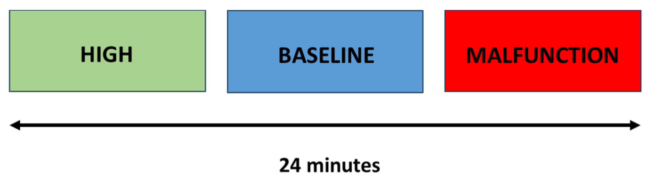
Figure 2.
Overview of the ATC sector and summary of automations additional functionalities to the BASELINE condition on the RADAR interface.
Figure 2.
Overview of the ATC sector and summary of automations additional functionalities to the BASELINE condition on the RADAR interface.
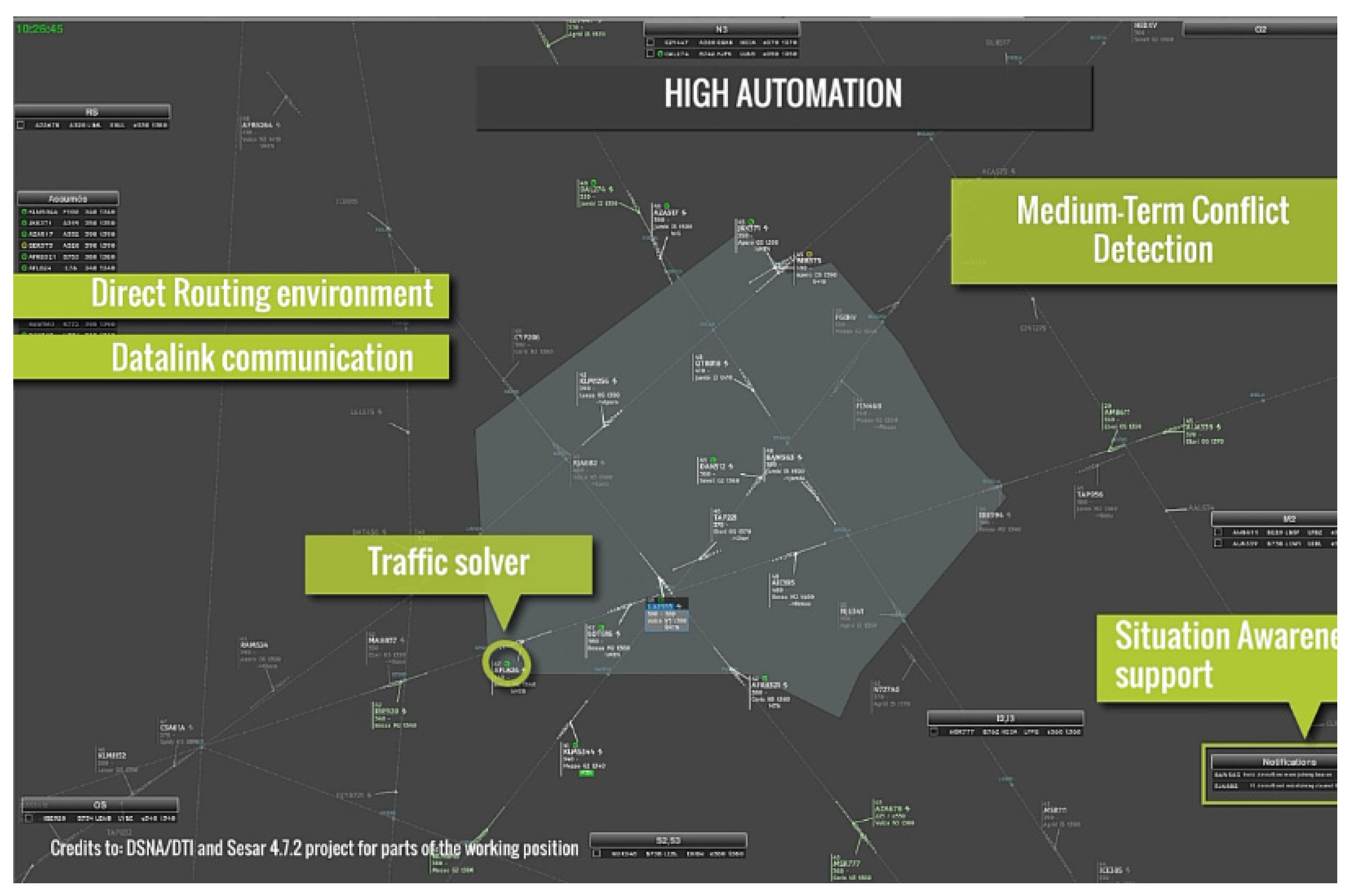
Figure 3.
Graphical representation of the HPE model characterisation. Each HF can be modelled by a coefficient calculated through the combination of its PageRank, Graph Density and Shannon Entropy. These coefficients (coloured lines) define a vertex of a polygon. The area of such a polygon is the HPE measure (dashed lines).
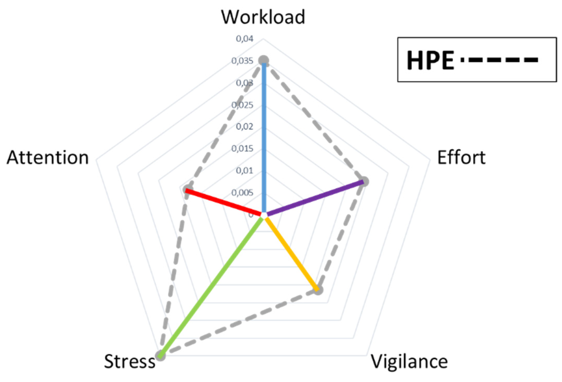

Table 1.
Order model (n) selected for each participant.
| Participant ID | Model order (n) |
|---|---|
| S1 | 7 |
| S2 | 5 |
| S3 | 8 |
| S4 | 9 |
| S5 | 9 |
| S6 | 7 |
| S7 | 4 |
| S8 | 11 |
| S9 | 9 |
| S10 | 5 |
| S11 | 7 |
| S12 | 11 |
| S13 | 7 |
| S14 | 4 |
| S15 | 5 |
| S16 | 10 |
| S17 | 6 |
Disclaimer/Publisher’s Note: The statements, opinions and data contained in all publications are solely those of the individual author(s) and contributor(s) and not of MDPI and/or the editor(s). MDPI and/or the editor(s) disclaim responsibility for any injury to people or property resulting from any ideas, methods, instructions or products referred to in the content. |
© 2026 by the authors. Licensee MDPI, Basel, Switzerland. This article is an open access article distributed under the terms and conditions of the Creative Commons Attribution (CC BY) license (http://creativecommons.org/licenses/by/4.0/).
Copyright: This open access article is published under a Creative Commons CC BY 4.0 license, which permit the free download, distribution, and reuse, provided that the author and preprint are cited in any reuse.


