
Submitted:
17 February 2026
Posted:
25 February 2026
You are already at the latest version
Abstract
Energy management systems under dynamic electricity pricing require fast and cost-optimal control strategies for the optimization of flexible loads such as heating, ventilation, and air conditioning (HVAC) systems and refrigeration units. While Mixed-Integer Linear Programming (MILP) can compute theoretically optimal control trajectories, its practical application is limited due to computationally expensive optimization, leading to limited real-time applicability, and its dependence on accurate forecasts of electrical loads and other relevant time-series signals including disturbances. This paper proposes a supervised imitation learning (IL) framework that learns to imitate MILP-optimal setpoint trajectories for a conventional proportional (P) controller using only electricity price signals and temporal features. Our IL model predicts setpoint trajectories in an open-loop manner without direct state feedback and a subsequent conventional P-controller provides closed-loop robustness in a two-stage control structure. In this study, our approach is validated for electrical load shifting of a refrigeration system in an industrial warehouse, including a systematic benchmark of multiple IL models. MILP achieves a cost reduction of 21.07% relative to baseline and serves as a theoretical upper bound. Among IL models, sequence-based architectures achieve the highest savings, with Transformer and Long Short-Term Memory (LSTM) models closely approximating MILP behavior, reaching 19.33% and 19.28% respectively. A closed-loop reinforcement learning (RL) controller achieves 19.69% savings and is included as an additional benchmark, while heuristic strategies reach at most 14.43% savings. From a computational perspective, IL models enable fast training and real-time inference, with Transformer inference requiring 526 ns per prediction compared to 22.8 s for a single MILP optimization. This makes the proposed approach well suited for real-time and edge computing applications. Overall, the results demonstrate that the proposed supervised IL approach can achieve near-optimal control performance with substantially reduced computational effort, providing a scalable and cost-efficient solution for energy management.
Keywords:
imitation learning
; supervised learning
; optimal control
; energy management
; dynamic electricity pricing
; transformer
; industrial warehouse
1. Introduction
Reducing carbon dioxide emissions and achieving global climate targets require the large-scale integration of renewable energy sources into modern power grids. However, the intermittent and variable nature of renewable generation poses significant challenges for maintaining grid stability and balancing supply and demand [1]. To address these challenges, energy management on the demand side has gained increasing importance, as flexible consumers can adapt their operation to support grid stability and reduce overall energy costs [2]. Traditionally, energy management systems have relied on classical heuristics, proportional-integral (PI) controllers, or model predictive control (MPC) approaches based on MILP and related optimization techniques [3]. Although MILP-based MPC formulations can guarantee global optimality under given model assumptions [4], their computational complexity often hinders their deployment in real-time and large-scale control applications, necessitating trade-offs between optimality and computational efficiency [5].
In contrast, RL has shown promise for adaptive process control and demand response in energy systems [6], yet RL models typically require extensive training [7] and can destabilize physical systems during training, making direct deployment in safety-critical environments challenging [8]. Additionally, both optimization-based and learning-based approaches can face limited robustness under process uncertainty and coordination-related stability issues in closed-loop operation. On the other hand, heuristic or rule-based control strategies, though computationally efficient, tend to underutilize the available operational flexibility and rarely achieve near-optimal economic performance [9,10].
To overcome these limitations, two-stage or hierarchical control architectures have been introduced, combining the advantages of rule-based and optimization-based strategies to achieve improved performance and system stability [11,12]. In a two-stage control architecture, the lower stage operates in real time using simplified rule-based or heuristic logic to ensure fast and stable system response, while the upper stage performs computationally intensive optimization over longer horizons. Advanced methods such as MILP or RL are often applied at the upper level to generate optimal setpoints or scheduling targets for the lower controller. This hierarchical structure effectively combines the real-time feasibility of classical control with the decision quality of optimization and learning-based approaches, achieving a balance between responsiveness and overall energy efficiency [12,13].
In parallel, Transformer architectures [14] have revolutionized sequence modeling by efficiently capturing long-range temporal dependencies through self-attention mechanisms. Compared to recurrent neural networks and LSTM models, Transformers excel in learning context-dependent relationships across multiple time scales, properties that are highly desirable in energy management and process optimization tasks. Recent applications demonstrate their superiority in load and renewable forecasting [15,16,17,18,19], yet their application to real-time setpoint trajectory generation within two-stage control architectures for industrial energy management under dynamic pricing has received limited attention.
1.1. Related Works
In energy management systems operating under dynamic electricity pricing, MILP has proven to be a well-established and effective optimization approach. Kepplinger et al. [21] implemented a MILP-based model predictive control strategy combined with a physics-based system model derived from transient energy balances to enable load shifting of smart water boilers under dynamic pricing, achieving cost savings of around 12%. Similar MILP-based MPC approaches have been successfully investigated for energy management of electric vehicles [22,23], net-zero energy buildings [24], energy communities [25], and industrial manufacturing [26,27,28,29], reporting cost savings typically around 30% for electric vehicle charging, up to 40–50% for net-zero energy buildings, and around 10–25% for industrial applications, depending on system flexibility and pricing volatility. In addition to simulation-based studies, selected works have further validated MILP-based energy management strategies in real-world field tests, demonstrating their practical feasibility under realistic operating conditions [30,31].
In recent years, RL has also been explored for energy management problems in dynamic pricing environments. Afroosheh et al. [32] proposed a deep Q-network (DQN)–based home energy management system that directly controls the scheduling of household loads and a battery energy storage system under dynamic electricity pricing while respecting user comfort constraints, achieving energy cost reductions of about 12%. In Muriithi et al. [33], a DQN–based energy management system is proposed for a grid-tied PV–battery microgrid operating under dynamic electricity price signals. The RL agent directly controls battery charging and power exchange with the grid based on the observed system state. Depending on the considered use case, the proposed approach achieves energy cost reductions between 15% and 26%.
While the aforementioned studies apply RL directly at the power and scheduling level, other works employ hierarchical control structures, in which RL operates at a supervisory level. Jiang et al. [34] applied a DQN for building HVAC control under a time-of-use electricity tariff with demand charges, where the RL agent adjusts temperature setpoints at a supervisory level, while a conventional lower-level controller translates these setpoints into actual power consumption. Simulation results show total cost reductions of approximately 6–8% compared to a rule-based baseline. Vetter et al. [35] investigate multi-energy optimization in an energy community under real-time electricity pricing, comparing a MILP formulation with a RL approach. While the MILP controller is implemented with direct power control, the DQN-based method follows a two-stage control structure, in which high-level decisions are translated into low-level control actions. As a result, the MILP approach exhibits slightly higher flexibility and achieves marginally higher cost reductions (about 10%) compared to the RL controller (approximately 9%). In an industrial context, a supervisory energy management framework compared MILP and DQN as RL approach for load shifting in a food processing plant under dynamic electricity pricing [36]. Both approaches operate at a supervisory control level by optimizing control setpoints that are implemented by a lower-level controller, with MILP serving as an optimization benchmark and RL as a data-driven alternative. The results demonstrate energy cost reductions of 18% for the RL-based approach and 19% for the MILP-based strategy, indicating that RL can achieve performance close to optimization-based control in industrial demand response applications.
These energy management systems typically require load or renewable generation forecasts. Supervised learning (SL) models, particularly Transformer-based architectures, are therefore widely used for load and renewable forecasting tasks. Liu et al. [15] apply Transformer-based SL to forecast solar radiation, photovoltaic power, wind speed, and wind power, demonstrating the effectiveness of sequence models for renewable energy forecasting. Tian et al. [16] present a day-ahead probabilistic load forecasting framework that combines convolutional neural networks with Transformer architectures, achieving high accuracy even with limited historical data, particularly for weekend load profiles. Moosbrugger et al. [17] investigate electrical load forecasting for energy communities using transfer learning, benchmarking LSTM, Transformer, and other machine learning models, with the forecasts subsequently applied in MILP-based energy management. Similarly, two studies by Wohlgenannt et al. [18,19] investigate electrical and thermal load forecasting in the food processing industry as inputs for downstream MPC via MILP or RL.
While most studies employ SL for forecasting to support downstream optimization, other works explore SL-based approaches that are used directly as controllers. For example, Novak and Dragičević [37] apply supervised IL to approximate finite-set MPC in power electronic converters, reducing computational effort while maintaining control performance. In the energy domain, Gao et al. [38] propose an IL–based approach for online optimal power scheduling of a microgrid, where a neural network approximates a MILP policy under uncertain prices and renewable generation. Dinh and Kim [39] propose a MILP-based IL approach for HVAC control, where a deep neural network is trained on optimal control actions generated by an MILP solver. The learned controller operates without explicit load or weather forecasts, using real-time data and day-ahead electricity prices to minimize energy costs while maintaining thermal comfort. Simulation results show near-optimal performance compared to forecast-based MILP, MPC, and RL approaches.
1.2. Contributions
Despite significant progress in optimization- and learning-based energy management, several practically relevant limitations remain insufficiently addressed. First, many strategies depend on explicit load or generation forecasts, which increases modeling effort and sensitivity to prediction errors, and complicates the overall learning pipeline since forecasting and decision-making must be trained and tuned separately rather than learned end-to-end. Second, while SL has been widely adopted in control and automation, its use for price-driven energy management is still limited and predominantly targets direct power scheduling rather than controller-compatible setpoint manipulation, which better aligns with practice. Third, most learning-based approaches are designed as single-stage controllers, whereas their integration into two-stage architectures, where a supervisory layer optimizes setpoints for embedded low-level controllers, is rarely investigated. Finally, experimental evaluations often focus on comparisons to non-optimized baselines, while systematic benchmarking against rule-based and heuristic strategies commonly applied in real settings remains scarce. Motivated by these gaps, this work makes the following contributions:
- A Transformer-based IL model predicts optimal refrigeration setpoint trajectories directly from historical price and temporal data, removing the need for intermediate load or production forecasts.
- Viability of IL-based prediction is proven within a systematic comparison to the optimal trajectory.
- Comprehensive evaluation of sequence, non-sequence, and linear SL models highlights the importance of temporal and non-linear modeling.
- Combined with a lower-level P controller, the model ensures stable operation while achieving cost-optimal setpoints, facilitating practical industrial implementation.
2. Methods
This study investigates a two-stage optimal control approach for energy management under dynamic pricing in an industrial refrigerated warehouse. The cooling demand is supplied by the refrigeration system, whereas the aggregated thermal mass of stored goods, building structure, and equipment constitutes an intrinsic thermal energy storage. Allowing a temperature band between 0 °C and 5 °C provides flexibility that can be exploited for load shifting and energy cost optimization. Our control framework follows a two-stage structure as can be seen in Figure 1. In the upper layer, different optimization strategies determine the optimal temperature setpoint trajectory. This setpoint serves as the reference for a lower-level P controller, which regulates the refrigeration system to maintain the desired warehouse temperature. This hierarchical setup ensures both optimized operation and system stability.
Various control strategies are investigated for the upper-level optimization. MILP, RL, and heuristic control are used as benchmark methods, while a novel IL approach is proposed. All control strategies aim to shift the electrical load of the refrigeration plant to periods with lower electricity prices under hourly real-time pricing.
Figure 2 illustrates the overall architecture and highlights the structural difference between the different methods. MILP explicitly incorporates the physical model, price signal, and load forecast to compute an optimal setpoint trajectory, which is then translated into cooling power by the P-controller. The resulting historical optimal trajectories serve as training targets for the IL model. The IL models are trained on historical MILP optimization results to learn optimal control behavior from prior data. Once trained, the IL model directly maps price signal and time information to a setpoint trajectory, thereby approximating the MILP solution without solving an optimization problem online. This enables a computationally efficient surrogate of the original optimization-based controller. RL is used as a closed-loop benchmark, learning a control policy through direct interaction with the environment by maximizing cumulative economic reward, while heuristic strategies provide rule-based baseline controllers without optimization or learning. A constant setpoint temperature of 2.5 °C, representing the current operational practice, is used as a reference case. Hyperparameters of all IL and RL algorithms were tuned using Bayesian optimization to achieve optimal performance on the training set. Further details on the individual upper-layer control strategies are provided in the following subsections.
2.1. Data Acquisition and Processing
The case study is based on data from previous work [36]. Hourly data from May 2020 to April 2023 obtained from an industrial refrigerated warehouse is used. The dataset includes production data (mass flow of products entering the warehouse, ), ambient temperature (), the energy efficiency ratio of the refrigeration system (), and estimated heat gains from the ambient (). While production data and thermal losses are available in the dataset, they are only used for benchmarking the proposed IL approach and are not provided as direct inputs to the forecasting model. Hourly spot market prices from the Energy Exchange Austria (EXAA) [44] served as the dynamic price signal for the optimization process. The electricity price was assumed to be available on a day-ahead basis, as it is published at noon for the following day by the EXAA. The dataset was divided into two subsets: two years were used for training, while the remaining year was reserved for testing and performance evaluation of IL against MILP, RL, and heuristic control as benchmarks. All simulations and analyses were implemented in Python and are executed on a MacBook Pro M2 from 2023.
2.2. Industrial Warehouse Model
Figure 3 shows a schematic of the industrial warehouse of a food processing plant, which was developed and validated in previous work [36], in combination with the two-stage controller.
The model represents the warehouse as a lumped thermal capacity that includes both the building structure and the stored food. Heat gains from the ambient environment () and mass flows of incoming () and outgoing food products () are combined into a simplified heat flow . Cooling is provided by an industrial chiller controlled via a discrete-time P controller with saturation. The set point temperature can be adjusted within a predefined band , providing thermal flexibility that can be exploited for load shifting. The simplified warehouse temperature dynamics are described by the discrete-time energy balance:
The model parameters are listed in Appendix A. This model has been used as the environment for both RL and MILP-based optimization in previous work [36], and is reused here for evaluation.
2.3. Mixed-Integer Linear Programming
MILP provides the global optimal temperature setpoint trajectory, making it a strong benchmark for control performance. In this study, MILP is solved over a 36-hour prediction horizon, of which the first 24 hours are applied; the problem is then re-optimized in a rolling-horizon fashion. MILP outperforms other methods not only because perfect knowledge of the load is assumed, but also because it guarantees the global optimum, whereas IL, RL, or heuristic controllers can only approximate it. On the downside, MILP can become computationally expensive for problems with many binary variables and must be solved repeatedly for real-time operation. The full MILP formulation can be found in Appendix B. The MILP is formulated and solved using Gurobi [46]. Here, MILP is used as one reference benchmark to evaluate the performance of the IL models.
2.4. Supervised Imitation Learning Models
In this work, imitation learning is implemented in the form of supervised behavior cloning, where optimal MILP-generated setpoint trajectories serve as expert demonstrations. The learning problem is therefore formulated as a supervised regression task that directly maps electricity price and temporal features to optimal setpoint trajectories. The models considered in this study include sequence-based models (LSTM, Transformer), tree-based models (DecisionTree, RandomForest, ExtraTrees, GradientBoosting, AdaBoost, XGBoost, LightGBM), instance-based models (KNN), kernel-based models (SVR, KernelRidge), and linear models (LinearRegression, LinearSVR, Ridge, Lasso, ElasticNet, BayesianRidge, SGD, Huber, PassiveAggressive, PLS). The control policy is learned end-to-end without an explicit load forecasting step. The model maps electricity prices and temporal features directly to control setpoints, avoiding forecast-induced errors and additional model maintenance. The input features include:
- Electricity price at the current timestep.
- Hour of the day encoded as sine and cosine functions to capture daily periodicity.
- Weekday encoded as a one-hot vector to represent weekly patterns.
- Day of the year encoded as sine and cosine functions to capture seasonality.
All feature values are standardized based on the mean and the standard deviation from the training dataset via z-transform:
In addition, the electricity price is first min-max normalized for each day before standardization:
The target of the prediction is the P-controller setpoint, constrained between 0 °C and 5 °C. All target values are standardized based on the training dataset. The optimal setpoint trajectories used as training targets were obtained by solving the corresponding MILP problems on the training data.
Model training was conducted using the historical MILP solutions as targets and the mean absolute error (MAE) as loss function, which is defined as follows:
The training dataset covers two years of operation and the remaining year is reserved for testing.
Hyperparameters for all models were tuned using Bayesian optimization with 50 trials, employing 5-fold cross-validation on the training set and a parameter grid specified in Appendix D. This procedure was applied individually for each model to maximize prediction accuracy on the validation folds.
The performance was evaluated on four levels. First, the economic impact of the predicted setpoint trajectories was quantified using the industrial warehouse model. The trajectories were implemented in the simulation environment, and the resulting operational costs were compared to a non-optimized reference scenario in which a conventional proportional P-controller operates with a constant temperature setpoint. This comparison directly quantifies the achievable cost reductions under dynamic electricity pricing.
Second, the quality of the predicted setpoint trajectories was evaluated using standard regression metrics, including MAE, root Mean Square Error (RMSE), , and symmetric mean absolute percentage error (sMAPE), computed on the test set. These metrics assess the accuracy of the predicted setpoints independently of their economic effect. The error metrics are defined as:
Third, computational efficiency was evaluated by measuring both training time and inference time, providing insight into the practical applicability of each model for real-time operation and edge deployment.
Fourth, the robustness of the proposed approach was assessed by verifying whether each method consistently fulfills all temperature constraints throughout the entire test horizon.
2.5. Deep Reinforcement Learning
A DQN was implemented as a benchmark following the approach described in previous studies [19,35,36]. The network structure illustrates the interaction between the agent and the environment through states, actions, and rewards. The DQN framework comprises a policy network for action selection and a target network for Q-value estimation. To enhance learning efficiency and stability, experience replay with mini-batch sampling is employed, and soft updates are applied to the target network. The implementation builds on the original deep Q-learning algorithm introduced by Mnih et al. [40] and incorporates improvements proposed by Van Hasselt et al. [42], namely the separation of policy and target networks. Soft target updates, as described by Lillicrap et al. [45], further stabilize training, while experience replay ensures more efficient and stable learning, consistent with the original DQN methodology [40]. In contrast to the previous work [36], as first modification the planning horizon has been extended to 36 hours; however, at each decision point (0:00), only the first 24 hours of the optimized trajectory are applied. The state, action, and reward definitions follow [36], with the second modification that the load forecast was removed from the state representation to enable a fair comparison with the IL models. Consequently, the RL agent must implicitly capture and predict the underlying load behavior through its learned policy, rather than relying on an external forecasting module. Optimized hyperparameters were adopted from the earlier study [19]. The DQN was implemented using PyTorch [48].
2.6. Heuristic Approaches
Simple heuristic methods were implemented as baseline approaches to provide additional benchmarks for evaluating the performance of the IL models. The heuristics considered in this study include a day-night strategy and price-based approaches using daily mean, median, or min-max normalization. The day-night heuristic applies a fixed daily pattern, with lower setpoints during the night (0–6 h and 18–24 h) and higher setpoints during the day (6–18 h), independent of the electricity price. For each day, the mean or median price is computed; hours with prices above this threshold are assigned a high setpoint (5 °C), and hours below are assigned a low setpoint (0 °C). This encourages higher temperatures during low-price periods and lower temperatures during high-price periods. The min-max heuristic normalizes the daily electricity price to the range [0,1] and linearly scales the setpoint to a defined range (0–5 °C). Hours with the lowest prices are mapped to the lowest setpoints, and hours with the highest prices are mapped to the highest setpoints, providing a continuous price-dependent setpoint trajectory.
2.7. Ablation Study
An ablation study was conducted to assess the contribution of individual feature groups used by the Transformer model. In each experiment, one complete feature block was removed from the input while keeping all other model settings unchanged. Interdependent features, such as sine and cosine encodings of temporal variables, were always removed jointly to ensure consistency.
2.8. Exploration of Additional Feature Candidates
An exploratory analysis was conducted to examine whether incorporating additional system-level information beyond electricity prices and temporal encodings improves model performance. Candidate features were added individually to the baseline Transformer model and evaluated using the same training and validation procedure as in the main experiments. The following system-level feature candidates were considered:
- Ambient temperature (current and lagged)
- Thermal load (current and lagged)
3. Results and Discussion
3.1. Cost Savings
Figure 4 summarizes the achieved cost reductions for all evaluated control strategies relative to the non-optimized baseline, grouped by model family and represented by their best-performing model per class. The optimized hyperparameters are described in Appendix C. The MILP solution provides the global optimum, achieving a cost reduction of 21.07% and serving as a theoretical upper bound, since it is computed under perfect foresight of system states, cooling demand, and external heat gains. Among IL approaches, sequence-based models clearly outperform other model families. The Transformer achieves a cost reduction of 19.33%, while the LSTM attains a similar improvement, highlighting that capturing temporal dependencies is essential for cost-optimal control under dynamic electricity pricing. Reinforcement learning (DQN) achieves a slightly higher cost reduction of 19.69%, closely approaching the MILP optimum. This performance is enabled by its closed-loop formulation but comes at the cost of substantially higher training effort and system complexity, and is therefore used primarily as a benchmark in this study. Tree-based, kernel-based, and instance-based models form a second performance tier, achieving cost reductions around 17%. While clearly inferior to sequence models, they significantly outperform heuristic approaches. Price-based heuristics such as Mean, Median, and MinMaxPrice already achieve moderate cost reductions (13–15%) with minimal effort. In contrast, the Day–Night heuristic increases total costs, illustrating that rigid, time-based strategies can be counterproductive under flexible electricity pricing. This highlights the necessity of price-aware and temporally adaptive control strategies. Linear and generalized linear models achieve less than 10% cost reduction and are consistently outperformed even by simple heuristics, indicating that linear modeling assumptions are insufficient to capture the nonlinear and temporal structure of the problem. For completeness, the full numerical results for all evaluated models are summarized in Appendix E.
While aggregated results compare economic performance across model families, a detailed temporal analysis is required to assess control quality. Figure 5 therefore presents system trajectories over three representative days for the MILP reference and the Transformer. The Transformer closely follows the overall structure of the MILP solution, resulting in similar power trajectories and cost accumulation, with minor deviations reflecting its prediction inaccuracies. Note that the MILP assumes perfect knowledge of the system behavior, the future thermal load, and disturbances and therefore represents a theoretical upper bound.
3.2. Prediction Quality
Figure 6 relates prediction accuracy, measured by sMAPE, to the achieved cost reduction for all evaluated approaches. A clear overall trend can be observed: models with lower prediction errors generally achieve higher cost savings. Sequence-based models, particularly the Transformer and LSTM, combine low prediction errors with high economic performance. Tree-based and instance-based models show moderate prediction accuracy and form a dense cluster with intermediate cost reductions, while linear and generalized linear models exhibit the highest errors and the weakest economic performance. RL constitutes a notable exception to this general trend: despite exhibiting the highest prediction errors with respect to the MILP reference trajectory, it achieves the greatest cost savings. This apparent contradiction can be explained by two factors. First, due to saturation effects of the lower-level P controller, different setpoint values can lead to identical cooling power, meaning that deviations from the MILP setpoint do not necessarily translate into different electrical load behavior. Second, unlike imitation learning (IL) models that aim to replicate the MILP trajectory in an open-loop fashion, the DQN follows a closed-loop control strategy and directly optimizes the economic reward through interaction with the environment. Consequently, although its temperature trajectory deviates from the MILP reference, it induces comparable load-shifting behavior and achieves competitive - even superior - economic performance. Overall, this observation underscores that prediction accuracy alone is not a sufficient indicator of economic performance. Different control strategies can yield similar cost reductions while exhibiting fundamentally different operational behaviors.
Detailed prediction metrics for all evaluated models are provided in Appendix F.
3.3. Computational Efficiency
Figure 7 illustrates the trade-off between achieved cost reduction and inference time for all evaluated approaches. The MILP solution requires optimization times on the order of seconds and is therefore probably not the best choice for real-time operation, particularly on edge devices with limited computational resources. In contrast, all IL models and RL achieve inference times several orders of magnitude lower, ranging from nanoseconds for linear models to microseconds for tree-based, kernel-based, and sequence models. Among IL approaches, the Transformer achieves near-optimal cost reductions while maintaining sub-microsecond inference times. Tree-based and kernel-based models also provide fast inference but achieve lower cost savings, while linear and generalized linear models, despite their minimal computational cost, perform poorly in terms of economic outcomes.
Figure 8 relates cost reduction to training time. All IL models require only seconds for training (up to 18 s), which is substantially faster than solving a single MILP instance for one day. RL requires significantly longer training times, on the order of tens of minutes, as the agent must learn the control policy through interaction and exploration rather than direct supervision. Note that while the MILP optimizer itself does not require training, it relies on an external load forecast. If this forecast is generated using deep learning, it introduces an additional training pipeline and effort that is comparable to training the IL models. A potential limitation of IL is that training assumes the availability of historical MILP reference trajectories; if these had to be generated online, training time would increase accordingly, whereas inference time would remain unaffected. Overall, all IL models are well suited for real-time deployment on edge devices with limited computational resources, with the Transformer offering the most favorable balance between training effort, inference speed, and achieved cost reduction.
Detailed training and inference times for all evaluated models are reported in Appendix G.
3.4. Temperature Constraint Violations
The temperature control over the test year was analyzed for all models, with deviations beyond the target setpoint plus a small tolerance (±0.25 °C) counted as violations. The results, summarized in Table 1, indicate that MILP, RL, and the heuristic approaches remained almost perfectly within the allowable range, exhibiting zero violations, with the base model showing only a minimal spread of 0.21 °C. Sequence models also closely tracked the setpoint. The Transformer model, which achieved the highest cost savings, exhibited zero violations, while the LSTM recorded only two rare violations, with a maximum temperature of 5.29 °C, just 0.04 °C above the upper bound, caused by the proportional gain of the controller rather than model extrapolation. In contrast, linear models such as LinearRegression, Ridge, Lasso, ElasticNet, BayesianRidge, and LinearSVR were more prone to violations due to their extrapolative behavior, with LinearSVR reaching up to 157 violations. Kernel-based methods exhibited even more extreme deviations. For example, KernelRidge recorded 205, 27, and 232 violations for different metrics, with maximum and minimum temperatures of 6.69 °C and -1.68 °C, respectively, highlighting its strong tendency to exceed the allowable bounds. Tree-based and boosting models were generally stable, with only a few exceptions observed for GradientBoosting, XGBoost, and LightGBM. Overall, the results show that IL can reliably maintain the temperature within the allowed bounds. Using a two-stage approach, where IL predicts the setpoint for the P controller, the Transformer model, for example, delivers fast and accurate predictions, achieves substantial cost savings, and robustly respects all temperature limits. Models prone to extrapolation could be further constrained by explicitly limiting setpoints to the 0–5 °C range. This approach clearly outperforms methods that directly control the power, which are more likely to violate operational constraints.
3.5. Ablation Study
Table 2 summarizes the results of the ablation study for the Transformer model. Removing the electricity price signal causes the strongest performance degradation, increasing operational costs by 4.20% relative to the reference model. Removing temporal encodings results in smaller cost penalties: omitting weekday information increases costs by 1.15%, while excluding day-of-the-year or hour-of-the-day features leads to penalties below 0.5%. Overall, temporal structure supports performance, but electricity price information is the dominant factor for economic optimization under dynamic pricing.
3.6. Exploration of Additional Feature Candidates
Table 3 reports the impact of additional system-level feature candidates on predictive accuracy and operational costs. None of the evaluated features consistently improves economic performance compared to the reference Transformer model.
Marginal improvements in sMAPE are observed for some feature configurations, but these do not translate into lower operational costs. In several cases, predicted costs are slightly higher than for the reference model, although the differences are not statistically significant. Even when all candidate features are combined, no further performance gains are achieved. Overall, the results indicate that the proposed price-driven approach already captures the most relevant information for generating cost-optimal setpoint trajectories. Incorporating additional system-level features increases model complexity and data requirements without providing measurable economic benefits.
3.7. Practical Applicability, Limitations and Future Research Directions
The proposed setpoint optimization framework is applicable to a wide range of energy systems that can be represented by setpoint-based control and storage-like dynamics. Beyond the investigated refrigeration system, potential application domains include heat pumps, hot water boilers, thermal storage systems, and battery energy storage systems operating under dynamic electricity pricing. The ability of the Transformer to generate entire setpoint trajectories directly from price and temporal signals enables effective load shifting without relying on explicit forecasts or continuous state feedback.
Despite the promising results, several limitations must be considered. The IL models rely on optimal MILP trajectories for training, which requires solving computationally expensive optimization problems under perfect information. However, this dependency does not preclude practical deployment, as MILP optimization can be performed periodically on centralized servers, while the trained IL models enable fast inference on resource-constrained edge devices.
Future research should therefore focus on three main directions. First, hybrid learning strategies that combine MILP with RL are promising, for example by injecting MILP-generated trajectories into the replay buffer of RL agents to accelerate training and improve convergence. Second, the development of generalized or so-called foundation models trained on representative load and storage profiles could enable privacy-preserving optimization without requiring feedback of system-specific measurements, while transfer learning could be used to adapt such models to individual systems when data sharing is permitted. Third, real-world validation under practical operating conditions, including disturbances, communication delays, and long-term system drift, remains essential to assess robustness and industrial applicability.
Addressing these aspects is key to transferring data-driven setpoint optimization from simulation studies to scalable, privacy-aware, and robust real-world energy management systems.
4. Conclusions
This study demonstrated the effectiveness of supervised IL to optimize the setpoints of an industrial refrigeration system. By predicting optimal setpoint trajectories directly with the help of historical price signals and temporal features, the proposed framework eliminates the need for intermediate load forecasts required for MILP or feedback loops required for RL. The results confirm that the Transformer model can replicate near-globally optimal behavior with high accuracy, achieving cost savings of 19.33%, thereby approaching the theoretical upper bound of 21.07% achieved by the MILP formulation. However, the MILP benchmark assumes perfect knowledge of both system dynamics and future load profiles, representing an idealized scenario that is not attainable in real-world applications. While RL achieved slightly higher savings (19.69%), the Transformer offers a distinct advantage in implementation simplicity and computational efficiency. With an inference time of just 526 ns, compared to over 22 seconds for a single MILP optimization, the model enables scalable, real-time control even on resource-constrained hardware. Unlike linear and kernel-based models, which frequently violated temperature constraints due to extrapolation errors, the Transformer model maintained the warehouse temperature strictly within the allowed bounds without a single violation throughout the test year. This demonstrates that sequence-based SL models can safely manage physical constraints when paired with a standard lower-level controller. In conclusion, the Transformer as supervised IL model represents a robust and cost-effective alternative to traditional MILP and RL approaches. It successfully bridges the gap between theoretical optimization and practical application, offering a scalable solution for data-driven energy management.
Author Contributions
Conceptualization, P.W., V.V., L.M., M.K., E.E. and P.K.; methodology, P.W., V.V., L.M., M.K., E.E and P.K; software, P.W., L.M.; validation, P.W., L.M., E.E. and P.K.; formal analysis, P.W., L.M., E.E. and P.K.; investigation, P.W.; resources, P.K.; data curation, P.W.; writing—original draft preparation, P.W.; writing—review and editing, P.W., V.V., L.M., E.E., M.K. and P.K.; visualization, P.W., V.V. and E.E.; supervision, M.K. and P.K.; project administration, P.K.; funding acquisition, P.K. All authors have read and agreed to the published version of the manuscript.
Funding
Philipp Wohlgenannt was funded by the European Union under the programme “Investment in Growth and Jobs (IBW) / European Regional Development Fund (ERDF) & Just Transition Fund (JTF) Austria 2021–2027” and the State of Vorarlberg. Peter Kepplinger and Lukas Moosbrugger gratefully acknowledge the financial support from the Austrian Research Promotion Agency FFG for the Hub4FlECs project (COIN FFG 898053).
Data Availability Statement
The datasets presented in this article are not readily available because they include confidential data from our project partner Rupp Austria GmbH. Requests to access the datasets should be directed to peter.kepplinger@fhv.at.
Acknowledgments
The authors are grateful to the project partner Rupp Austria GmbH for providing the data and all the fruitful discussions. The authors used ChatGPT to improve the clarity, grammar, and style of the manuscript and to assist with routine programming tasks. The tool was not employed to generate scientific content, analyze data, or design the research methods.
Conflicts of Interest
The authors declare no conflicts of interest.
Abbreviations
The following abbreviations are used in this manuscript:
| DQN | Deep Q-network |
| EXAA | Energy exchange Austria |
| HVAC | Heating, ventilation and air conditioning |
| IL | Imitation Learning |
| LSTM | Long Short-Term Memory |
| MPC | Model predictive control |
| MAE | Mean absolute error |
| MILP | Mixed-Integer Linear Programming |
| P | Proportional |
| PI | Proportional-integral |
| RL | Reinforcement learning |
| RMSE | Root Mean Square Error |
| SL | Supervised Learning |
| sMAPE | Symmetric mean absolute percentage error |
Appendix A. Model Parameters

Table A1.
Model Parameters.
| Parameter | Value |
|---|---|
| 4 360 MJ/K | |
| 500 t | |
| 1 260 t | |
| 480 J/(kg K) | |
| 3 270 J/(kg K) | |
| 4.938 | |
| 202 511 W | |
| 0 W | |
| 5 °C | |
| 0 °C | |
| 60 s | |
| 500 000 W/K |
Appendix B. MILP Formulation
The following decision variables are defined for the model:
- is the set point temperature of the warehouse during the time period p.
- is the warehouse temperature at the time point t.
- is the output signal of the P-controller before saturation during the time period p.
- is a helper variable for calculating the saturation during the time period p.
- are binary variables to calculate the saturation during the time period p.
- is the electrical power consumption of the industrial refrigeration system p.
The following time series are needed as inputs:
- is the price signal during the time period p.
- is the heat flow rate of the load during the time period p.
The following parameters are needed additionally:
- is the length of a time period.
- is the initial warehouse temperature at the time point 0.
- is the thermal capacity of the warehouse.
- is the energy efficiency ratio of the industrial refrigeration system.
- proportional factor of the controller.
- is the minimum electrical power.
- is the maximum electrical power.
- is the minimum set point temperature.
- is the maximum set point temperature.
- N is the number of time periods.
- and are big M constraints.
The following sets are defined:
- is the set of time period indices.
- is the set of time point indices.
- is a set to index of every hour of a day.
- is a set to index every minute in a hour.
The optimization problem minimizing the total costs can be written as:
Appendix C. Optimal Hyperparameters
Table A2.
Hyperparameters of all evaluated IL and RL models. Parameters not listed use library defaults.
Table A2.
Hyperparameters of all evaluated IL and RL models. Parameters not listed use library defaults.
| Model | Key hyperparameters |
|---|---|
| Transformer | model_size=2k, epochs=80 |
| LSTM | model_size=10k, epochs=60 |
| DecisionTree | max_depth=10, min_samples_split=15, min_samples_leaf=4, |
| max_features=None | |
| RandomForest | , max_depth=32, min_samples_split=3, |
| min_samples_leaf=1, max_features=None, bootstrap=True | |
| ExtraTrees | , max_depth=37, min_samples_split=8, |
| min_samples_leaf=1, max_features=None | |
| GradientBoosting | , learning_rate=0.080, max_depth=8, |
| subsample=0.951, min_samples_split=7, min_samples_leaf=4 | |
| AdaBoost | , learning_rate=0.032, loss=linear |
| XGBoost | , learning_rate=0.0205, max_depth=10, |
| subsample=0.854, colsample_bytree=0.860, | |
| reg_alpha=, reg_lambda=, | |
| min_child_weight=1.53 | |
| LightGBM | , learning_rate=0.0191, num_leaves=176, |
| subsample=0.765, colsample_bytree=0.734, | |
| reg_alpha=0.00742, reg_lambda=0.0423, | |
| min_child_samples=5 | |
| KNN | , weights=uniform, leaf_size=35, |
| SVR | kernel=RBF, , , scale |
| KernelRidge | kernel=laplacian, , |
| LinearRegression | – |
| LinearSVR | – |
| Ridge | |
| Lasso | |
| ElasticNet | , -ratio=0.970 |
| BayesianRidge | , , |
| , | |
| SGDRegressor | max_iter=1000, tol=, penalty=l1, |
| HuberRegressor | , |
| PassiveAggressive | max_iter=1000, tol=, , |
| PLSRegression | |
| DQN | num_episodes=10 000, batch_size=64, replay_memory=100 000, |
| eps_decay=10 000, network_depth=4, network_width=512 |
Appendix D. Hyperparameter Search Spaces
The following lists summarize the hyperparameter search spaces used in this study. All ranges are inclusive; log indicates logarithmic sampling. Unless otherwise stated, the same random seed (random_state) was used for all experiments to ensure reproducibility, and parallel execution was enabled by setting n_jobs = -1 where applicable.
Transformer and LSTM
- model_size
- epochs (step size 20)
Random Forest
- max depth
- min samples split
- min samples leaf
- max features
- bootstrap
Extra Trees
- max depth
- min samples split
- min samples leaf
- max features
Decision Tree
- max depth
- min samples split
- min samples leaf
- max features
Gradient Boosting
- learning rate (log)
- max depth
- subsample
- min samples split
- min samples leaf
AdaBoost
- learning rate (log)
- loss
XGBoost
- learning rate (log)
- max depth
- subsample
- colsample_bytree
- regα, regλ (log)
- min child weight (log)
- tree method = hist
LightGBM
- learning rate (log)
- num leaves
- max depth
- subsample
- colsample_bytree
- regα, regλ (log)
- min child samples
KNN
- weights
- leaf size
- (Minkowski metric)
Support Vector Regressor
- kernel
- (log)
- (log)
- degree (only if kernel = poly)
Kernel Ridge Regression
- kernel
- (log)
- (log) (only if kernel = rbf or laplacian)
- degree (only if kernel = poly)
- coef0 (only if kernel = poly)
Ridge Regression
- (log)
Lasso Regression
- (log)
Elastic Net
- (log)
- ratio
Bayesian Ridge
- (log)
SGD Regressor
- (log)
- penalty
- max_iter = 1 000, tol =
Huber Regressor
- (log)
- max_iter = 1 000
Passive Aggressive Regressor
- (log)
- (log)
- max_iter = 1 000, tol =
Partial Least Squares
Deep Q-Network (DQN)
- Number of training episodes
- Batch size
- Replay buffer size
- Exploration decay steps
- Network depth (number of hidden layers)
- Network width (neurons per hidden layer)
Appendix E. Detailed Cost and Performance Results
Table A3.
Total costs and relative cost reduction compared to Base.
| Family | Model | Costs [EUR] | Costs vs Base [%] |
|---|---|---|---|
| Base | - | 141 705 | 0.00 |
| Global Optimum | MILP | 111 848 | 21.07 |
| Sequence | Transformer | 114 314 | 19.33 |
| LSTM | 114 388 | 19.28 | |
| Tree-based | DecisionTree | 118 561 | 16.33 |
| RandomForest | 117 730 | 16.92 | |
| ExtraTrees | 117 128 | 17.34 | |
| GradientBoosting | 117 402 | 17.15 | |
| AdaBoost | 123 655 | 12.74 | |
| XGBoost | 117 320 | 17.21 | |
| LightGBM | 117 388 | 17.15 | |
| Instance | KNN | 117044 | 17.40 |
| Kernel | SVR | 119 655 | 15.56 |
| KernelRidge | 117 231 | 17.27 | |
| Linear | LinearRegression | 128 117 | 9.59 |
| LinearSVR | 127 970 | 9.69 | |
| Ridge | 128 134 | 9.58 | |
| Lasso | 128 117 | 9.59 | |
| ElasticNet | 128 117 | 9.59 | |
| BayesianRidge | 128 136 | 9.58 | |
| SGD | 128 309 | 9.45 | |
| Huber | 128 012 | 9.66 | |
| PassiveAggressive | 129 351 | 8.72 | |
| PLS | 128 116 | 9.59 | |
| RL | DQN | 113 800 | 19.69 |
| Heuristics | DayNight | 146 884 | -3.65 |
| Mean | 120 784 | 14.76 | |
| Median | 123 226 | 13.04 | |
| MinMaxPrice | 121 258 | 14.43 |
Appendix F. Detailed Prediction Results
Table A4.
Prediction metrics evaluated against the optimal MILP reference trajectory.
| Family | Model | MAE | RMSE | sMAPE [%] | |
|---|---|---|---|---|---|
| Sequence | Transformer | 0.77 | 1.19 | 0.42 | 31.95 |
| LSTM | 0.78 | 1.23 | 0.38 | 32.91 | |
| Tree-based | DecisionTree | 0.90 | 1.24 | 0.37 | 38.27 |
| RandomForest | 0.89 | 1.23 | 0.38 | 37.80 | |
| ExtraTrees | 0.88 | 1.21 | 0.40 | 37.77 | |
| GradientBoosting | 0.90 | 1.24 | 0.37 | 37.87 | |
| AdaBoost | 1.03 | 1.27 | 0.34 | 42.60 | |
| XGBoost | 0.89 | 1.23 | 0.38 | 37.73 | |
| LightGBM | 0.90 | 1.25 | 0.36 | 38.10 | |
| Instance | KNN | 0.88 | 1.20 | 0.41 | 38.17 |
| Kernel | SVR | 0.93 | 1.20 | 0.41 | 38.86 |
| KernelRidge | 0.96 | 1.30 | 0.31 | 40.46 | |
| Linear | LinearRegression | 1.08 | 1.34 | 0.26 | 48.33 |
| LinearSVR | 1.07 | 1.36 | 0.24 | 46.06 | |
| Ridge | 1.08 | 1.34 | 0.26 | 48.33 | |
| Lasso | 1.08 | 1.34 | 0.26 | 48.33 | |
| ElasticNet | 1.08 | 1.34 | 0.26 | 48.33 | |
| BayesianRidge | 1.08 | 1.34 | 0.26 | 48.33 | |
| SGD | 1.08 | 1.34 | 0.26 | 48.58 | |
| Huber | 1.08 | 1.34 | 0.26 | 48.01 | |
| PassiveAggressive | 1.09 | 1.35 | 0.25 | 47.97 | |
| PLS | 1.08 | 1.34 | 0.26 | 48.33 | |
| RL | DQN | 1.34 | 1.77 | -0.28 | 49.79 |
Appendix G. Computational Performance: Training and Inference
Table A5.
Training and inference times grouped by model family. Inference per prediction is averaged over all test steps.
Table A5.
Training and inference times grouped by model family. Inference per prediction is averaged over all test steps.
| Family | Model | Train time | Runtime per prediction |
|---|---|---|---|
| Global Optimum | MILP | - | 22.8 s |
| Sequence | Transformer | 3.003 s | 526 ns |
| LSTM | 3.931 s | 1 µs | |
| Tree-based | DecisionTree | 0.033 s | 47 ns |
| RandomForest | 2.437 s | 9 µs | |
| ExtraTrees | 0.752 s | 6 µs | |
| GradientBoosting | 12.210 s | 5 µs | |
| AdaBoost | 1.362 s | 4 µs | |
| XGBoost | 1.038 s | 4 µs | |
| LightGBM | 0.215 s | 25 µs | |
| Instance | KNN | 0.004 s | 15 µs |
| Kernel | SVR | 4.457 s | 222 µs |
| KernelRidge | 17.736 s | 121 µs | |
| Linear | LinearRegression | 0.003 s | 89 ns |
| LinearSVR | 0.057 s | 36 ns | |
| Ridge | 0.001 s | 17 ns | |
| Lasso | 0.369 s | 17 ns | |
| ElasticNet | 0.363 s | 16 ns | |
| BayesianRidge | 0.004 s | 12 ns | |
| SGD | 0.009 s | 19 ns | |
| Huber | 0.008 s | 9 ns | |
| PassiveAggressive | 0.005 s | 18 ns | |
| PLS | 0.005 s | 21 ns | |
| RL | DQN | 20 min | 2 ms |
References
- Ergun, S.; Dik, A.; Boukhanouf, R.; Omer, S. Large-Scale Renewable Energy Integration: Tackling Technical Obstacles and Exploring Energy Storage Innovations. Sustainability 2025, 17, 1311. [CrossRef]
- Panda, S.; Mohanty, S.; Rout, K.; Sahu, B.; Parida, S. M.; Samanta, I.; Bajaj, M.; Piecha, M.; Blažek, V.; Prokop, L. A Comprehensive Review on Demand Side Management and Market Design for Renewable Energy Support and Integration. Energy Reports 2023, Volume 10, 2228–2250. [CrossRef]
- Eyimaya, S. E.; Altin, N. Review of Energy Management Systems in Microgrids. Applied Sciences 2024, 14 (3), 1249. [CrossRef]
- Integer Programming: 2nd Edition. In Integer Programming; John Wiley & Sons, Ltd, 2020; pp 1–34. [CrossRef]
- Yaghoubi, E.; Yaghoubi, E.; Maghami, M. R.; Rahebi, J.; Zareian Jahromi, M.; Ghadami (Melisa Rahebi), R.; Yusupov, Z. A Systematic Review and Meta-Analysis of Model Predictive Control in Microgrids: Moving Beyond Traditional Methods. Processes 2025, 13 (7), 2197. [CrossRef]
- Vázquez-Canteli, J. R.; Nagy, Z. Reinforcement Learning for Demand Response: A Review of Algorithms and Modeling Techniques. Applied Energy 2019, 235, 1072–1089. [CrossRef]
- Bakare, M. S.; Abdulkarim, A.; Zeeshan, M.; Shuaibu, A. N. A Comprehensive Overview on Demand Side Energy Management towards Smart Grids: Challenges, Solutions, and Future Direction. Energy Informatics 2023, 6 (1), 4. [CrossRef]
- García, J.; Fernández, F. A Comprehensive Survey on Safe Reinforcement Learning. The Journal of Machine Learning Research. 2015, 16 (1), 1437–1480.
- Bakare, M. S.; Abdulkarim, A.; Shuaibu, A. N.; Muhamad, M. M. Energy Management Controllers: Strategies, Coordination, and Applications. Energy Informatics 2024, 7 (1), 57. [CrossRef]
- Elmouatamid, A.; Ouladsine, R.; Bakhouya, M.; EL KAMOUN, N.; Khaidar, M.; Zine-dine, K. Review of Control and Energy Management Approaches in Micro-Grid Systems. Energies 2020, 14, 168. [CrossRef]
- Yassuda Yamashita, D.; Vechiu, I.; Gaubert, J.-P. Two-Level Hierarchical Model Predictive Control with an Optimised Cost Function for Energy Management in Building Microgrids. Applied Energy 2021, 285, 116420. [CrossRef]
- Shan, Y.; Ma, L.; Yu, X. Hierarchical Control and Economic Optimization of Microgrids Considering the Randomness of Power Generation and Load Demand. Energies 2023, 16, 5503. [CrossRef]
- Villalón, A.; Rivera, M.; Salgueiro, Y.; Muñoz, J.; Dragičević, T.; Blaabjerg, F. Predictive Control for Microgrid Applications: A Review Study. Energies 2020, 13 (10). [CrossRef]
- Vaswani, A.; Shazeer, N.; Parmar, N.; Uszkoreit, J.; Jones, L.; Gomez, A.N.; Kaiser, Ł.; Polosukhin, I. Attention is All You Need. In Proceedings of the 31st International Conference on Neural Information Processing Systems—NIPS’17, Long Beach, CA, USA, 4–9 December 2017; Curran Associates Inc.: Red Hook, NY, USA, 2017; pp. 6000–6010.
- Liu, J.; Fu, Y. Renewable Energy Forecasting: A Self-Supervised Learning-Based Transformer Variant. Energy 2023, 284, 128730. [CrossRef]
- Tian, Z.; Liu, W.; Jiang, W.; Wu, C. CNNs-Transformer Based Day-Ahead Probabilistic Load Forecasting for Weekends with Limited Data Availability. Energy 2024, 293, 130666. [CrossRef]
- Moosbrugger, L.; Seiler, V.; Wohlgenannt, P.; Hegenbart, S.; Ristov, S.; Eder, E.; Kepplinger, P. Load Forecasting for Households and Energy Communities: Are Deep Learning Models Worth the Effort? arXiv July 18, 2025. [CrossRef]
- Wohlgenannt, P.; Moosbrugger, L.; Hegenbart, S.; Huber, G.; Kolhe, M.; Kepplinger, P. Optimal Sizing and Operation of a Battery Energy Storage System for Demand Response in a Food Processing Plant Using Deep Learning for Load Forecasting. In Data Science – Analytics and Applications. Proceedings of the 6th International Data Sciene Conference - iDSC2025; Springer Nature: Salzburg, Austria, 2025. [CrossRef]
- Wohlgenannt, P.; Moosbrugger, L.; Vetter, V.; Hegenbart, S.; Kolhe, M.; Eder, E.; Kepplinger, P. Energy Cost and Emission Optimization in Food Industry Using Deep Reinforcement Learning and Transformer-Based Load Forecasting. Energy Conversion and Management: X 2025, 28, 101364. [CrossRef]
- Yassuda Yamashita, D.; Vechiu, I.; Gaubert, J.-P. Two-Level Hierarchical Model Predictive Control with an Optimised Cost Function for Energy Management in Building Microgrids. Applied Energy 2021, 285, 116420. [CrossRef]
- Kepplinger, P.; Huber, G.; Petrasch, J. Autonomous Optimal Control for Demand Side Management with Resistive Domestic Hot Water Heaters Using Linear Optimization. Energy and Buildings 2015, 100, 50–55. [CrossRef]
- Ireshika, M. A. S. T.; Preissinger, M.; Kepplinger, P. Autonomous Demand Side Management of Electric Vehicles in a Distribution Grid. In 2019 7th International Youth Conference on Energy (IYCE); 2019; pp 1–6. [CrossRef]
- Ireshika, M. A. S. T.; Kepplinger, P. Uncertainties in Model Predictive Control for Decentralized Autonomous Demand Side Management of Electric Vehicles. Journal of Energy Storage 2024, 83, 110194. [CrossRef]
- Baumann, C.; Wohlgenannt, P.; Streicher, W.; Kepplinger, P. Optimizing Heat Pump Control in an NZEB via Model Predictive Control and Building Simulation. Energies 2025, 18, 100. [CrossRef]
- Seiler, V.; Moosbrugger, L.; Huber, G.; Kepplinger, P. Assessing Model Predictive Control for Energy Communities’ Flexibilities. In e-nova 2024 Intelligente Energie- und Klimastrategien: Energie - Gebäude - Umwelt BAND 27; Holzhausen, 2024. [CrossRef]
- Wohlgenannt, P.; Preißinger, M.; Kolhe, M. L.; Kepplinger, P. Demand Side Management of a Battery-Supported Manufacturing Process with On-Site Generation. In 2022 IEEE 7th International Energy Conference (ENERGYCON); IEEE: Riga, Latvia, 2022. [CrossRef]
- Wohlgenannt, P.; Huber, G.; Rheinberger, K.; Preißinger, M.; Kepplinger, P. Modelling of a Food Processing Plant for Industrial Demand Side Management. In HEAT POWERED CYCLES 2021 Conference Proceedings; Heat Powered Cycles: Bilbao, Spain, 2022; pp 638–649. [CrossRef]
- Wohlgenannt, P.; Huber, G.; Rheinberger, K.; Kolhe, M.; Kepplinger, P. Comparison of Demand Response Strategies Using Active and Passive Thermal Energy Storage in a Food-Processing Plant. Energy Rep. 2024, 12, 226–236. [CrossRef]
- Saffari, M.; de Gracia, A.; Fernández, C.; Belusko, M.; Boer, D.; Cabeza, L. F. Optimized Demand Side Management (DSM) of Peak Electricity Demand by Coupling Low Temperature Thermal Energy Storage (TES) and Solar PV. Applied Energy 2018, 211, 604–616. [CrossRef]
- Kepplinger, P.; Huber, G.; Petrasch, J. Field Testing of Demand Side Management via Autonomous Optimal Control of a Domestic Hot Water Heater. Energy and Buildings 2016, 127, 730–735. [CrossRef]
- Baumann, C.; Huber, G.; Alavanja, J.; Preißinger, M.; Kepplinger, P. Experimental Validation of a State-of-the-Art Model Predictive Control Approach for Demand Side Management with a Hot Water Heat Pump. Energy and Buildings 2023, 285, 112923. [CrossRef]
- Afroosheh, S.; Esapour, K.; Khorram-Nia, R.; Karimi, M. Reinforcement Learning Layout-Based Optimal Energy Management in Smart Home: AI-Based Approach. IET Gener. Transm. Distrib. 2024, 18, 2509–2520. [CrossRef]
- Muriithi, G.; Chowdhury, S. Deep Q-Network Application for Optimal Energy Management in a Grid-Tied Solar PV-Battery Microgrid. J. Eng. 2022, 2022, 422–441. [CrossRef]
- Jiang, Z.; Risbeck, M. J.; Ramamurti, V.; Murugesan, S.; Amores, J.; Zhang, C.; Lee, Y. M.; Drees, K. H. Building HVAC Control with Reinforcement Learning for Reduction of Energy Cost and Demand Charge. Energy Build. 2021, 239, 110833. [CrossRef]
- Vetter, V.; Wohlgenannt, P.; Kepplinger, P.; Eder, E. Deep Reinforcement Learning Approaches the MILP Optimum of a Multi-Energy Optimization in Energy Communities. Energies 2025, 18 (17), 4489. [CrossRef]
- Wohlgenannt, P.; Hegenbart, S.; Eder, E.; Kolhe, M.; Kepplinger, P. Energy Demand Response in a Food-Processing Plant: A Deep Reinforcement Learning Approach. Energies 2024, 17 (24), 6430. [CrossRef]
- Novak, M.; Dragicevic, T. Supervised Imitation Learning of Finite-Set Model Predictive Control Systems for Power Electronics. IEEE Transactions on Industrial Electronics 2021, 68 (2), 1717–1723. [CrossRef]
- Gao, S.; Xiang, C.; Yu, M.; Tan, K. T.; Lee, T. H. Online Optimal Power Scheduling of a Microgrid via Imitation Learning. IEEE Transactions on Smart Grid 2022, 13 (2), 861–876. [CrossRef]
- Dinh, H. T.; Kim, D. MILP-Based Imitation Learning for HVAC Control. IEEE Internet of Things Journal 2022, 9 (8), 6107–6120. [CrossRef]
- Mnih, V.; Kavukcuoglu, K.; Silver, D.; Rusu, A. A.; Veness, J.; Bellemare, M.G.; Graves, A.; Riedmiller, M.; Fidjeland, A. K.; Ostrovski, G.; et al. Human-Level Control through Deep Reinforcement Learning. Nature 2015, 518, 529–533. [CrossRef]
- Watkins, C.J.C.H.; Dayan, P. Q-Learning. Mach. Learn. 1992, 8, 279–292. [CrossRef]
- van Hasselt, H.; Guez, A.; Silver, D. Deep Reinforcement Learning with Double Q-learning. In Proceedings of the Thirtieth AAAI Conference on Artificial Intelligence (AAAI-16), Phoenix, AZ, USA, 12–17 February 2016; pp.2094–2100. [CrossRef]
- Azuatalam, D.; Lee, W.-L.; de Nijs, F.; Liebman, A. Reinforcement Learning for Whole-Building HVAC Control and Demand Response. Energy AI 2020, 2, 100020. [CrossRef]
- DAY-AHEAD PREISE. Available online: https://markttransparenz.apg.at/de/markt/Markttransparenz/Uebertragung/EXAA-Spotmarkt (accessed on 23 September 2024).
- Lillicrap, T.P.; Hunt, J.J.; Pritzel, A.; Heess, N.; Erez, T.; Tassa, Y.; Silver, D.; Wierstra, D. Continuous Control with Deep Reinforcement Learning. arXiv 2019, arXiv:1509.02971.
- Gurobi version 11.0. Available online: https://www.gurobi.com (accessed on 23 September 2024).
- scikit-learn version 1.6.0. Available online: https://scikit-learn.org/ (accessed on 1 December 2025).
- Pytorch version 2.1.1. Available online: https://pytorch.org (accessed on 23 September 2024).
- Optuna version 4.4. Available online: https://optuna.org (accessed on 1 December 2025).
Figure 1.
Two stage control architecture showing the upper level controller (e.g. IL) and the P-controller for the lower level.
Figure 1.
Two stage control architecture showing the upper level controller (e.g. IL) and the P-controller for the lower level.
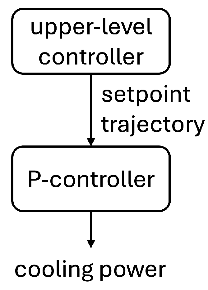
Figure 2.
Overall control framework: MILP-based reference optimization and alternative control approaches comprising IL, RL, and heuristic strategies. IL is trained on historical MILP setpoint trajectories, RL learns via closed-loop reward maximization, and heuristics provide rule-based baseline control.
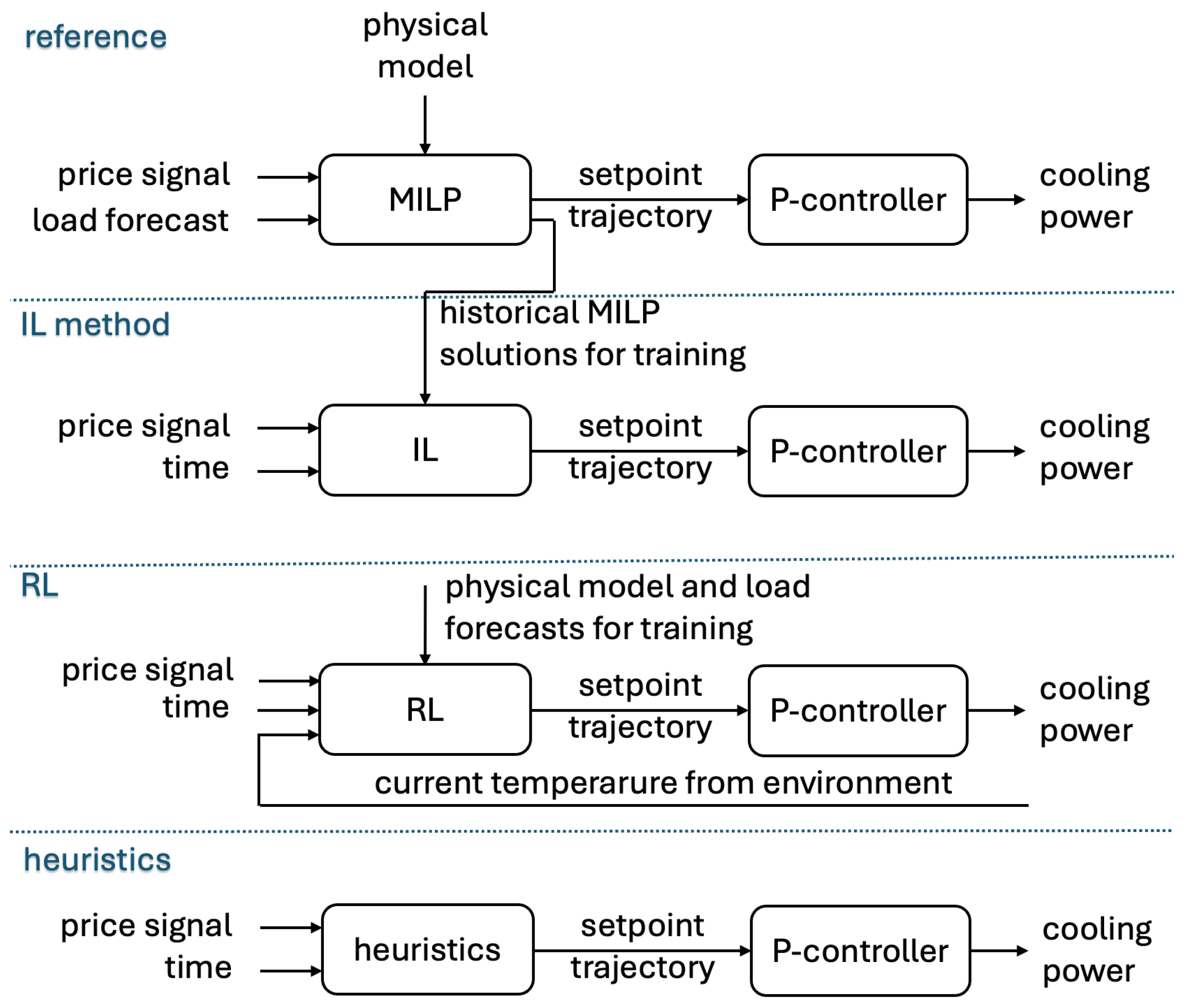
Figure 3.
Schematic representation of the industrial warehouse model used to evaluate different upper-layer control strategies.
Figure 3.
Schematic representation of the industrial warehouse model used to evaluate different upper-layer control strategies.
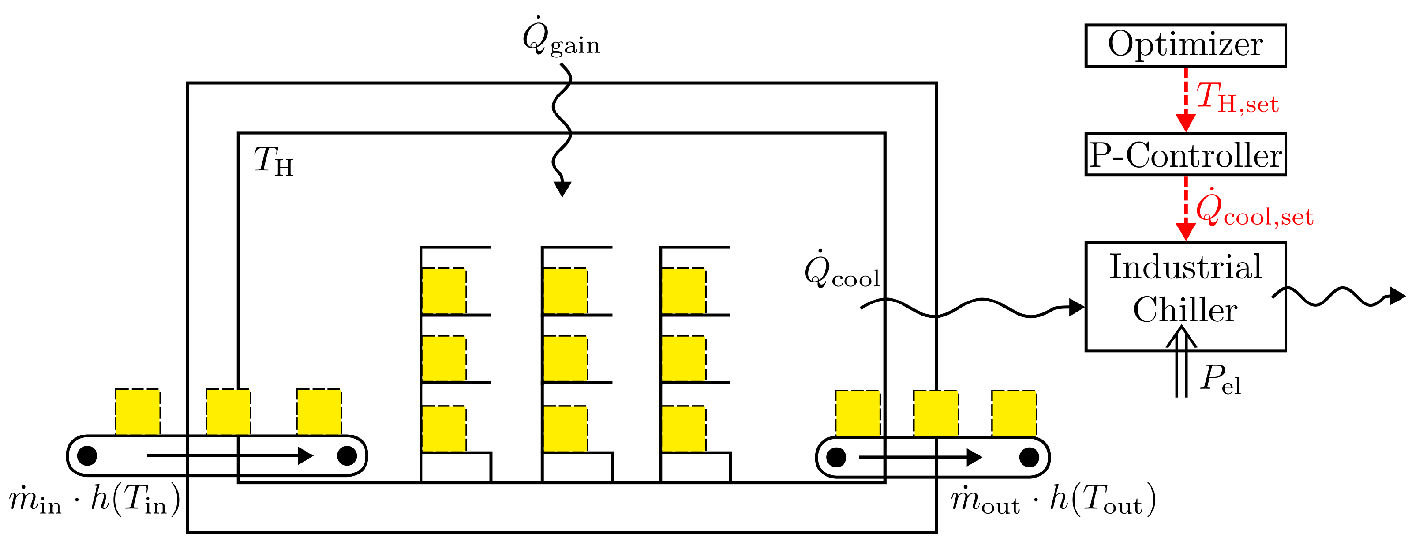
Figure 4.
Achieved electricity cost reduction relative to the non-optimized reference scenario for all evaluated control strategies. Results are grouped by model family and show the best-performing configuration per group. The MILP solution represents the global optimum and serves as an upper bound for achievable cost savings.
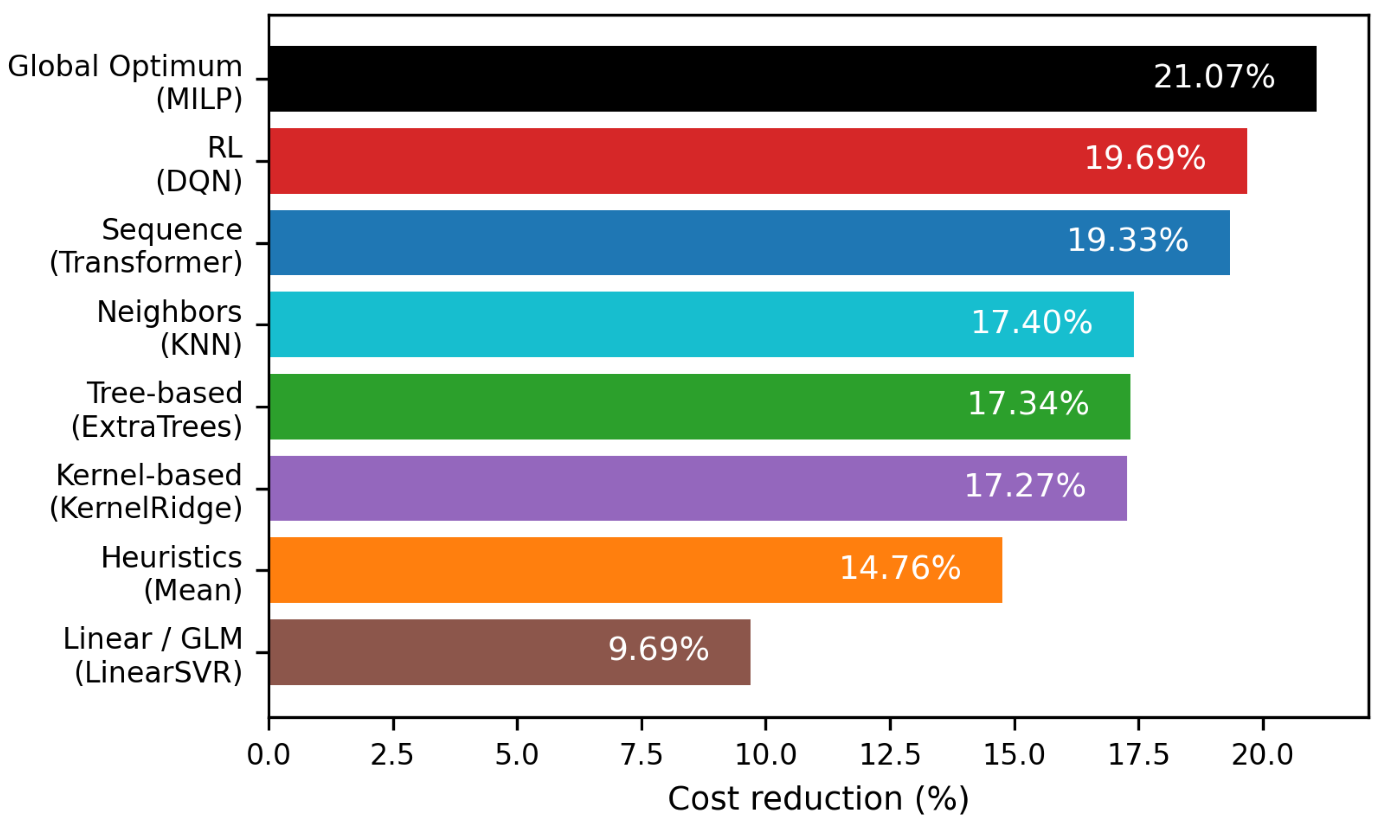
Figure 5.
Comparison of system trajectories over three representative days of the MILP benchmark and the Transformer-based IL model. Shown are the resulting warehouse temperature, the electrical power consumption, and the electricity price signal, illustrating similarities and differences in load-shifting behavior.
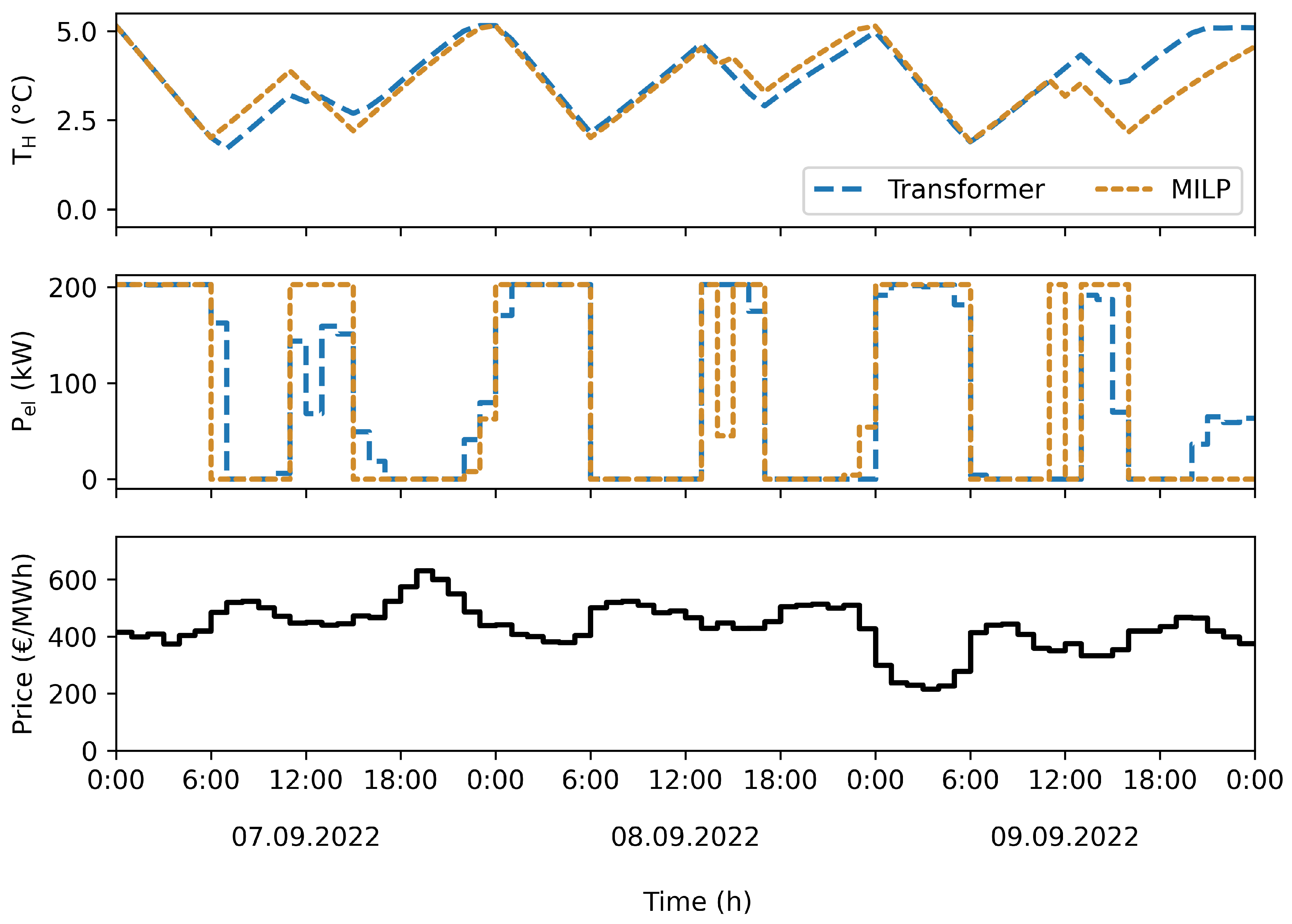
Figure 6.
Relationship between prediction accuracy, measured by sMAPE with respect to the MILP reference trajectory, and achieved cost reduction for all evaluated control strategies.
Figure 6.
Relationship between prediction accuracy, measured by sMAPE with respect to the MILP reference trajectory, and achieved cost reduction for all evaluated control strategies.
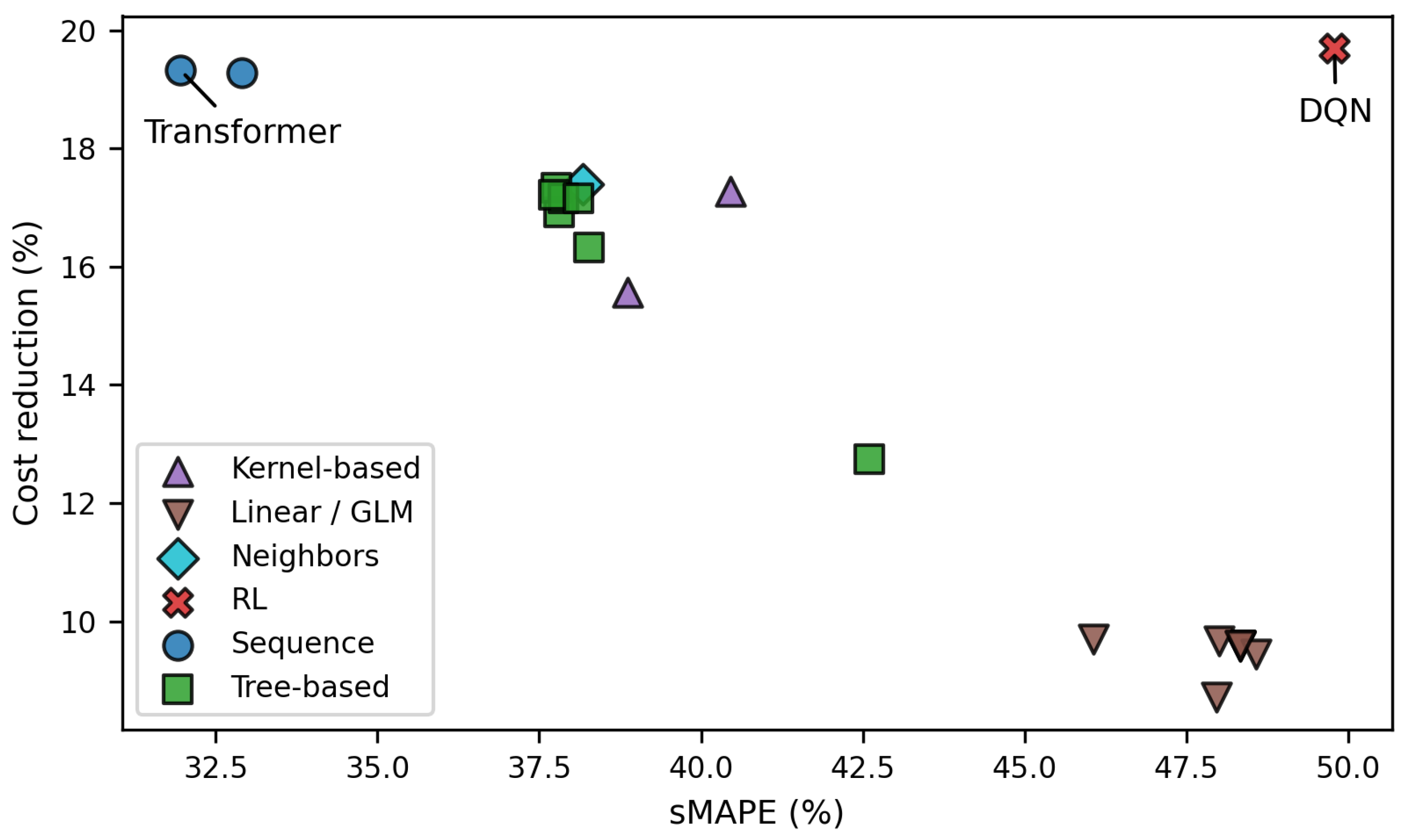
Figure 7.
Trade-off between achieved electricity cost reduction and inference time per prediction for the evaluated control strategies.
Figure 7.
Trade-off between achieved electricity cost reduction and inference time per prediction for the evaluated control strategies.
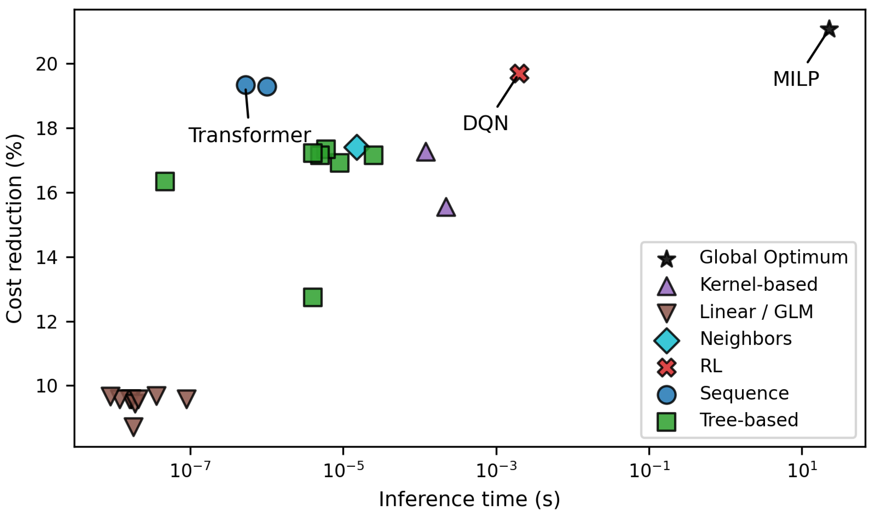
Figure 8.
Relationship between achieved cost reduction and model training time.
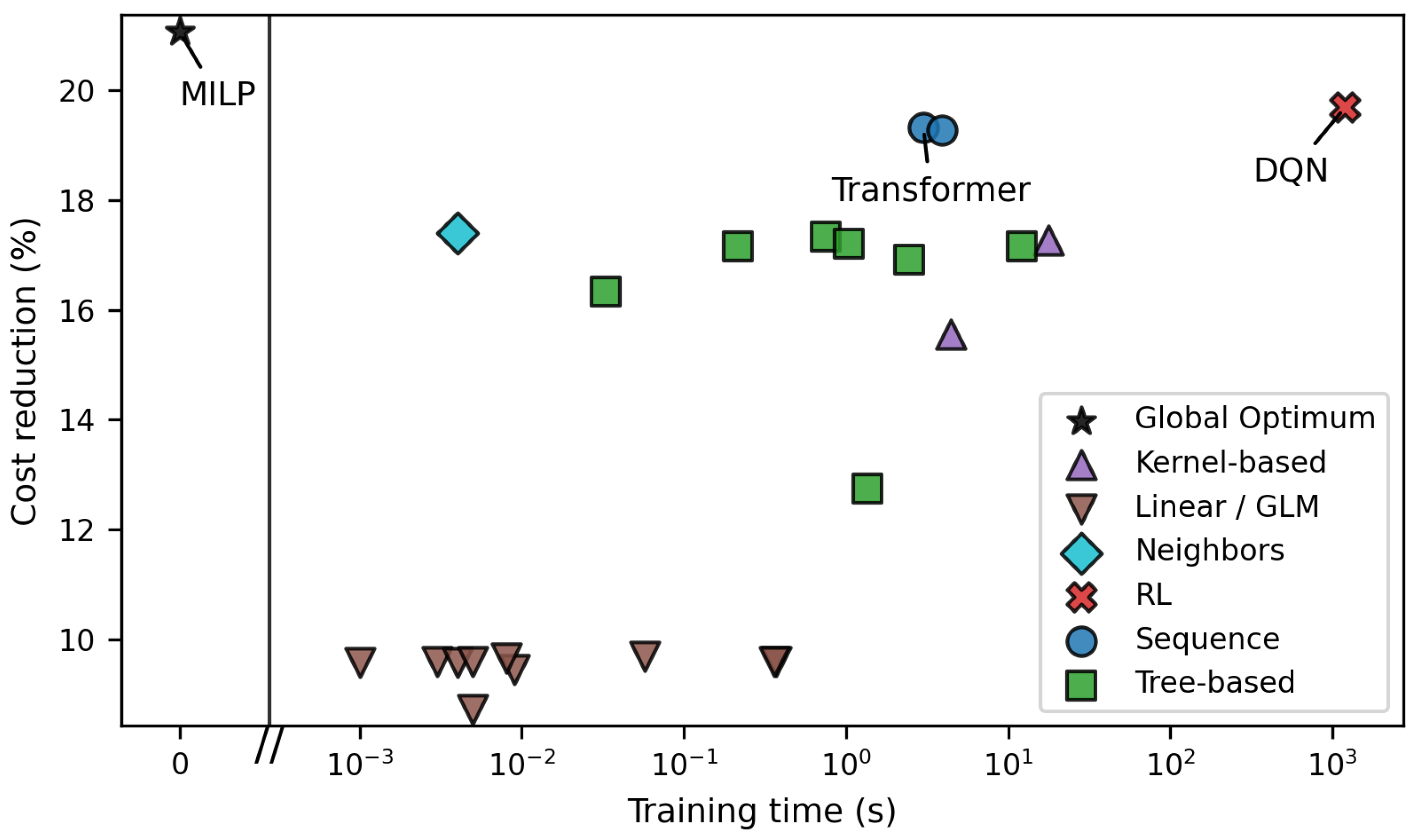
Table 1.
Temperature violations of all models over the test year, grouped by model family.
| Family | Model | > +5.25 | < -0.25 °C | Sum | Max (°C) | Min (°C) |
|---|---|---|---|---|---|---|
| Base | - | 0 | 0 | 0 | 2.71 | 2.50 |
| Global Optimum | MILP | 0 | 0 | 0 | 5.17 | 0.08 |
| Sequence | Transformer | 0 | 0 | 0 | 5.22 | 0.14 |
| LSTM | 2 | 0 | 2 | 5.29 | 0.06 | |
| Tree-based | DecisionTree | 0 | 0 | 0 | 5.17 | 0.16 |
| RandomForest | 0 | 0 | 0 | 5.12 | 0.16 | |
| ExtraTrees | 0 | 0 | 0 | 5.12 | 0.14 | |
| GradientBoosting | 25 | 0 | 25 | 5.55 | 0.14 | |
| AdaBoost | 0 | 0 | 0 | 4.56 | 1.86 | |
| XGBoost | 1 | 0 | 1 | 5.27 | -0.13 | |
| LightGBM | 2 | 0 | 2 | 5.31 | -0.06 | |
| Neighbors | KNN | 0 | 0 | 0 | 5.14 | 0.10 |
| Kernel | SVR | 30 | 3 | 33 | 6.81 | -1.47 |
| KernelRidge | 205 | 27 | 232 | 6.69 | -1.68 | |
| Linear | LinearRegression | 32 | 0 | 32 | 5.43 | 1.43 |
| LinearSVR | 157 | 0 | 157 | 5.66 | 1.28 | |
| Ridge | 32 | 0 | 32 | 5.43 | 1.44 | |
| Lasso | 32 | 0 | 32 | 5.43 | 1.43 | |
| ElasticNet | 32 | 0 | 32 | 5.43 | 1.43 | |
| BayesianRidge | 32 | 0 | 32 | 5.42 | 1.44 | |
| SGD | 9 | 0 | 9 | 5.33 | 1.60 | |
| Huber | 49 | 0 | 49 | 5.46 | 1.43 | |
| PassiveAggressive | 51 | 0 | 51 | 5.45 | 1.63 | |
| PLS | 36 | 0 | 36 | 5.43 | 1.44 | |
| RL | DQN | 0 | 0 | 0 | 5.16 | 0.06 |
| Heuristics | DayNight | 0 | 0 | 0 | 5.10 | 0.06 |
| Mean | 0 | 0 | 0 | 5.19 | 0.06 | |
| Median | 0 | 0 | 0 | 4.26 | 0.06 | |
| MinMaxPrice | 0 | 0 | 0 | 5.13 | 0.06 |
Table 2.
Ablation study for the Transformer model. Penalties are calculated relative to the Transformer model with all features and averaged over 50 runs. Slight numerical differences of the reference case arise due to independent training runs.
Table 2.
Ablation study for the Transformer model. Penalties are calculated relative to the Transformer model with all features and averaged over 50 runs. Slight numerical differences of the reference case arise due to independent training runs.
| Variant | sMAPE [%] | Costs [€] | Cost penalty [%] |
|---|---|---|---|
| reference/all | 32.57 | 114 274 | - |
| no EXAA price | 36.35 | 119 078 | 4.20 |
| no weekdays | 34.11 | 115 589 | 1.15 |
| no day of the year | 32.23 | 114 754 | 0.42 |
| no hour of the day | 34.11 | 114 660 | 0.34 |
Table 3.
Impact of additional feature candidates on predictive accuracy and costs for the Transformer model. Penalties are calculated relative to the Transformer model with the reference features and averaged over 50 runs. Slight numerical differences of the reference case arise due to independent training runs.
| Feature Set | sMAPE [%] | Predicted Costs [€] | Cost Penalty [%] |
|---|---|---|---|
| reference | 32.08 | 114 380 | - |
| with temperature | 32.06 | 114 388 | 0.01 |
| with lagged temperature | 32.09 | 114 463 | 0.07 |
| with thermal load | 32.04 | 114 474 | 0.08 |
| with lagged thermal load | 32.04 | 114 380 | 0.00 |
| with all candidates | 32.09 | 114 456 | 0.07 |
Disclaimer/Publisher’s Note: The statements, opinions and data contained in all publications are solely those of the individual author(s) and contributor(s) and not of MDPI and/or the editor(s). MDPI and/or the editor(s) disclaim responsibility for any injury to people or property resulting from any ideas, methods, instructions or products referred to in the content. |
© 2026 by the authors. Licensee MDPI, Basel, Switzerland. This article is an open access article distributed under the terms and conditions of the Creative Commons Attribution (CC BY) license (http://creativecommons.org/licenses/by/4.0/).
Copyright: This open access article is published under a Creative Commons CC BY 4.0 license, which permit the free download, distribution, and reuse, provided that the author and preprint are cited in any reuse.


