
Submitted:
11 June 2024
Posted:
11 June 2024
You are already at the latest version
Abstract
The climate crisis necessitates a global shift to achieve a secure, sustainable, and affordable energy system toward a green energy transition reaching climate neutrality by 2050. Because of this, renewable energy sources have come to the forefront and the research interest in microgrids which rely on distributed generation and storage systems has exploded. Furthermore, many new markets for energy trading, ancillary services, and frequency reserve markets have provided attractive investment opportunities in exchange for balancing the supply and demand of electricity. Artificial intelligence can be utilized to locally optimize energy consumption, trade energy with the main grid, and participate in these markets. Reinforcement learning (RL) is one of the most promising approaches to achieve this goal because it enables an agent to learn optimal behavior in a microgrid by executing specific actions that maximize the long-term reward signal/function. The study focuses on testing two optimization algorithms: logic-based optimization and reinforcement learning. This paper proposes an optimization algorithm based on reinforcement learning in an industrial microgrid that is capable of trading energy with the main grid, providing significant cost savings. The RL-based approach is implemented in Python based on real data from the site and in combination with MATLAB-Simulink to validate its results. The application of the RL algorithm achieved an average monthly cost saving of 20% compared to logic-based optimization and 86% savings compared to not using any optimization. These findings contribute to digitalization and decarbonization of energy technology and support fundamental goals and policies of the European Green Deal.
Keywords:
EMS
; PPO
; BESS
; Optimization Algorithm
; Peak Shaving
; Price Arbitrage
1. Introduction
Clean energy sources such as hydropower, wind energy, and solar energy are gradually replacing more conventional energy sources based on fossil fuels and coal. This shift is a result of the environmental duty to become sustainable and reduce carbon emissions, in addition to the outcomes of economic and technological progress. Therefore, as the globe moves towards more sustainable solutions, the significance of microgrids and distributed generation, especially those that use and incorporate more renewable energy sources, has grown. There has been a significant shift in how the power system operates thus microgrids emerged as the new method of managing distributed generation. The term "microgrid," is defined according to the US Department of Energy as "A group of interconnected loads and distributed energy resources within clearly defined electrical boundaries that act as a single controllable entity with respect to the grid" [1]. Industrial microgrids (IMGs) are made up of industrial loads, energy storage systems (ESS), and renewable energy sources and have different operational requirements compared to residential microgrids[2] [3]. Such kind of microgrids aid in lowering long-distance power transmission losses while simultaneously reducing the pollution from heavy industry [4]. IMGs are an effective instrument for adapting to diverse energy requirements. A Battery Energy Storage System (BESS), for example, may be controlled by a microgrid to provide different backup power and enhance the reliability of the IMG. [5].
An Energy Management System (EMS) is used to optimally coordinate the power exchange throughout the IMG and with the main grid, reducing energy costs while improving flexibility and energy efficiency[6][7] [8]. Designing and developing EMS algorithms for day-ahead and real-time scheduling is challenging because of the complexity of the microgrid, intermittent nature of DERs, and unpredictable load requirements [9][6]. Battery Energy Storage systems (BESS) can be effectively utilized to balance these demands and trade energy with the main grid based on the renewable production and price of electricity.
Energy Optimization in industrial microgrids has been extensively studied in the literature. Authors in [10] developed a day-ahead multi-objective optimization framework for industrial plant energy management, assuming that the facility had installed RESs. Meanwhile, [11] created an optimal energy management method in the industrial sector to minimize the total electricity cost with renewable generation, energy storage, and day-ahead pricing using state task network and mixed integer linear programming while [12] presented a demand response strategy to reduce energy for industrial facilities, using energy storage and distributed generation investigated under day-ahead, time-of-use, and peak pricing schemes. These studies utilized basic optimization approaches and did not utilize forecasting. On the other hand, [13] introduced an online EMS for an industrial facility equipped with energy storage. The optimization employed a rolling horizon strategy and used an artificial neural network model to forecast and minimize the uncertainty of electricity prices. The system solved a mixed-integer optimization problem based on the most recent forecast results for each sliding window, which helped in scheduling responsive demands. Additionally, [14] presented a real-time EMS that used a data distribution service that incorporated an online optimization scheme for microgrids with residential energy consumption and irradiance data from Florida. It utilized a feed-forward neural network to predict the power consumption and renewable energy generation. A review of energy optimization in industrial microgrids utilizing distributed energy resources is presented in [15].
Reinforcement learning has emerged as a method to solve complex problems with large state spaces. An RL agent starts with a random policy, which is a mapping between the observations (inputs) and the actions (outputs), and then incrementally learns to update and improve its policy using a reward signal that is given by the environment as an evaluation of the quality of the action performed. The goal of the agent is to maximize the reward signal over time. This can be achieved using a variety of methods but generally, there are two high-level approaches, learning through the value function, and learning through the policy. A value function is an estimate of the future rewards obtained by taking an action and then following a specific policy. RL agents can learn either by optimizing the value function, the policy, or both [16]. Actor-critic learning approaches make use of both the policy and the value function. The actor modifies the policy by updating the value function estimate provided by the critic.
Reinforcement learning has been used to optimize microgrids in the residential sector because it has proven to be a viable strategy for optimizing complex dynamic systems [17] [18]. For instance, a microgrid in Belgium saw a reduction in cost and an increase in efficiency when the Deep-Q-Network (DQN) technique was implemented in [19] assuming a fixed price of electricity. The suggested method in [20] generated three distinct consumption profiles according to the needs of the customers and used the Deep Deterministic Policy Gradient (DDPG) algorithm to produce a very profitable scheme. However, the results were only observed over a few weeks, and for one of the plans, the battery was simply discharged at the end, which does not demonstrate how the trained algorithm would function over an extended period of time. Several distinct reinforcement learning algorithms were compared over a ten-day period in using data from Finland and an enhanced version of the Advantage Actor-Critic algorithm (A3C++) achieved the best performance [21]. In a different instance, [22] reduced the operational cost by 20.75% using RL. More recently, Proximal Policy Optimization (PPO) has emerged as a powerful RL algorithms and was utilized in [23] and [24] to optimize energy cost in a microgrid with promising results. However, load forecasting was not included.
This paper builds on the existing research framework by combining PPO with machine learning-based load forecasting to produce an optimal solution for an industrial microgrid in Norway under different pricing schemes including day-ahead pricing, and peak pricing. It addresses the peak shaving and price arbitrage challenges by taking the historical data into the algorithm and making the decisions according to the pattern of energy consumption, battery characteristics, PV production, and energy price.
The paper is distributed into four different sections. The microgrid architecture is discussed in Section 2 with the components of the microgrid at the industrial site in Norway. In Section 3, the design and workflow of the EMS algorithms are discussed and the results from the algorithms are presented in Section 4 while Section 5 concludes the paper.
2. Microgrid Architecture
The microgrid at the industrial site in Norway is a grid-connected system with 200kWp of PV generation, a 1.1 MWh battery storage system, a 360kW electric vehicle charger, and two types of loads. The overall system diagram can be seen in Figure 1. There are several smart meters (denoted by SM) installed to record the energy flow. Load 1 and Load 2 are the main electricity loads, where load 1 is an industrial load while load 2 is a smaller load from an existing old building.
The 1.1 MW battery energy storage system (BESS) is used for backup energy supply and storage. This stored energy is sold back to the grid when the electricity prices are high. The 360kW electric vehicle (EV) charger is present at the facility to charge the electric lorries and trucks.
2.1. PV System
The PV system is distributed in three different areas in three buildings. The south building is a facade configuration with 44 panels with 310 watts each while the southeast building is equipped with 96 modules with an 11° inclination and with roof-mounted configuration. Similarly, the northwest building is configured with 74 solar panels with an 11° inclination towards the northwest. The PV system also contains 3 inverters to couple it with the IMG. Based on the irradiance in the area, the anticipated PV energy production throughout 2024 was calculated using PVSOL software, and the results are displayed in Figure 2. Table 1 shows the general parameters of the PV system.
2.2. Battery Energy Storage System
The BESS used is a 1.1 MWh container unit equipped with bidirectional inverters also called Power Conversion System (PCS). It is outfitted with high-precision sensors to monitor all its internal parameters such as temperature, humidity, voltage, and current, and protect against overcharging, flooding, or fire. This is achieved using a series of logical interlocks and a mix of hardware and software safeguards. The battery and inverter specifications are given in Table 2.
An essential component of controlling the energy transfer between the battery storage system and the electrical grid is the bidirectional inverter or Power Conversion System (PCS). Its primary job is to charge the batteries by converting alternating current (AC) from the IMG into direct current (DC), and vice versa. For applications such as peak shaving, where excess energy is kept during low demand times and released at peak demand to sustain grid operations, this bidirectional capability is essential.
The inverter or PCS system has the ability to operate in both grid-tied and off-grid modes. This system is adaptable for a range of energy storage requirements since it can handle broad battery voltage ranging from 600V to 900V, generate up to 500kW of nominal power, and support up to 8 battery strings. With an efficiency above 97%. For efficient thermal management, the PCS unit uses forced air cooling, which ensures peak performance even at full load.

Table 3.
Table showing Inverter Specifications.
| Parameters | Values |
|---|---|
| Rated Voltage | 400V (L-L) |
| Rated Frequency | 50/60 Hz |
| AC Connection | 3W+N |
| Rated Power | 2x500 kW |
| Rated Current Imax | 2x721.7 A |
| Power Factor | 0.8-1 (leading or lagging, load-dependent) |
In addition to the main components, the system also contains other IoT devices, smart meters, GPC (Grid Power Controller), etc. These devices function as a gateway to the battery system so that it can be controlled with the help of software programming. They operate on LINUX and use the MODBUS TCP protocol [25] for communication with local or remote servers and to send data to the cloud.
Figure 1, illustrates the four smart meters in the industrial microgrid out of which SM1 is a virtual smart meter while SM2, SM3, and SM4 are the physically present meters connected to the loads and DERs. These smart meters measure apparent power, active power, and reactive power using the true RMS value measurement (TRMS) up to the 63rd harmonic in all four quadrants [26].
3. Energy Management System
The basic block diagram of the energy management system is shown in Figure 3. It receives the measurements from the IMG, processes all the data, and uses different optimization algorithms to produce energy dispatch commands that are sent back to the IMG. These algorithms are explained in the following sections.
3.1. Data Acquisition and Processing
The EMS development steps are shown in Figure 4. The first step to developing an energy management system is to collect data from different components such as PV, battery storage system, grid, etc. The data can be collected using various sources such as smart meters, data loggers, a database or cloud system, or publicly available API services. The PV irradiance data was taken from PVSOL simulation software. Another important set of data to be read for the EMS development was the consumption data from the loads present at the industrial site and the grid import. Since the area is primarily a manufacturing site, the majority of its load or consumption is from heavy machines used for manufacturing. The load values and grid import values are collected using the Phoenix Contact smart meter [26].
The energy price data is collected from ’www.hvakosterstrommen.no’ website [27]. This website provides an open and free API to retrieve Norwegian electricity prices along with historical data. They collect the data from ENTSO-E in euros and convert it to the local currency using the latest exchange rate [28]. ENTSO-E is a transparency platform where data and information on electricity generation, transportation, and consumption are centralized and published for the benefit of the whole European market [28].
3.2. Data Analysis and Forecasting
The data analysis and forecasting part consisted of four main steps: data preparation and feature engineering, model training, forecasting and adjustment, and compilation and output. The initial step of this process is taking the historical data and arranging it in a specific format, removing outliers and missing values, etc. The data was collected on an hourly basis and is aggregated from different sources including PV production, battery state-of-charge, grid power import, and site load values as well as the hourly electricity prices. The forecasting process begins with loading historical data, time-based features are then prepared, and features and target variables are defined. A Random Forest Regressor model [29] is trained using this data.
The Random Forest Regressor is a meta estimator based on decision trees that employs averaging to increase prediction accuracy and manage over-fitting after fitting several decision tree regressors on different subsamples of the dataset. The Random Forest structure can be represented conceptually in Equation (1) as follows [30]:
Where:
- is the prediction function of the Random Forest.
- B is the number of trees.
- represents a single decision tree indexed by b, which is a function of the features X and random parameters .
Predictions are adjusted based on PV production before making a forecast for a specific month. Finally, the results are compiled and saved, completing the process.
Figure 5 shows the graph from forecasted data. It shows the grid import(denoted by red line) and site load(denoted by green line) of the site. The grid import is negative as time goes by because following the month of March, there is more PV production and due to this, more energy is supplied to the grid.
3.3. Logic-Based Optimization
A logic-based optimization algorithm was developed to use a benchmark and the flowchart of the algorithm is displayed in Figure 6. The energy price and battery SOC play an important role in the optimization process. The system starts by measuring the following important parameters: the power generated by the PV system (), the load/consumption (), the cost of energy (), the power imported from the grid (), and the initial state of charge of the battery (). The viability of using stored energy vs. grid energy is then evaluated based on economic factors, such as if the current cost of energy is less than a predetermined minimum ().
The system will not charge the battery to save expensive energy expenses if the cost is unfavorable and the battery SOC is below a maximum threshold (). Upon reaching a certain power threshold (), the system determines if it is necessary to use the grid to satisfy energy requirements. The battery health is maintained by the system maintaining the battery SOC above a minimum allowable level (). On the other hand, the algorithm will discharge the battery if the SOC is above . To maximize both economic and energy efficiency, the system additionally incorporates some logic to manage energy from the PV system and use it directly for the load or to charge the battery with any excess generation.
For peak shaving, the algorithm uses an energy management technique called "dynamic peak shaving" which is used to lower the greatest power demand or load in the system throughout the day. By setting a peak shaving threshold, the power demand, or grid import per hour is kept below a certain level. This is accomplished using a battery storage system to supplement the grid supply during times of high demand. Dynamic peak shaving aims to minimize energy expenses, prevent peak demand charges, and lessen the burden on the electrical system. The peak shaving threshold is dynamically determined using the maximum load estimate for each day. This algorithm is intended to run on a daily basis.
The algorithm determines the battery’s charge, discharge, or hold state each hour based on site load and projected energy price. It charges the battery when prices are low, ensuring it does not exceed maximum SOC, and discharges when prices are high or the site load surpasses the dynamic peak shaving level, maintaining SOC above the minimum. If neither condition is met, the battery remains in the "Hold" state. The algorithm adjusts the battery’s SOC and power output based on these decisions, ensuring SOC stays within operating limits and optimizing battery usage for cost and load needs. This process preserves battery efficiency and lifespan while managing energy flow.
3.4. Reinforcement Learning Algorithm
The reinforcement learning algorithm was developed using the same parameters to compare its output for cost saving with the results of the logic-based optimization. The RL agent was specifically designed to minimize costs associated with energy and peak load charges. It leverages a reinforcement learning (RL) algorithm [31], Proximal Policy Optimization (PPO) [32], implemented through the Stable Baselines3 library. The first step in developing the RL agent using the PPO algorithm was to build a custom environment, which is built on the OpenAI Gymnasium framework, which is a standard for developing and comparing reinforcement learning algorithms. This environment simulates the microgrid and allows the agent to control the battery storage system. It includes the battery actions; charging, discharging, and holding, and defines a discrete action space and a continuous observation space, where the state includes normalized values of forecasted site load, grid import, PV production, and battery SOC.
The proximal Policy Optimization algorithm works by iteratively enhancing its policy without introducing significant, harmful revisions. The clipped surrogate objective function, which has the following mathematical expression shown in Equation (2), is the approach used by the PPO algorithm to limit the undesirable policy changes [33].
where:
- is the probability ratio of the current policy to the old policy .
- is an estimator of the advantage function at timestep t.
- is a small value (e.g., 0.1 or 0.2) which defines the clipping range to keep the updates stable [33].
The objective of the RL agent is to identify the optimal strategy that reduces power costs while respecting operational limitations such as battery SOC and capacity. The RL agent is then trained for 50 million timesteps. The model gives feedback in the form of rewards during this process, which are intended to motivate cost-cutting behaviors. For example, the agent is rewarded when it takes advantage of cheap energy price hours to charge and minimizes grid usage by discharging during peak costs. It eventually learns how to maximize battery utilization for cost optimization by iteratively improving its policy.
Figure 7 shows the general diagram of the PPO algorithm. The actions are evaluated based on the rewards they generate, to minimize costs and maximize efficiency, and the system iteratively improves its decision-making strategy through continuous training episodes. During training, the agent is used in a simulation to calculate the best course of action (charge, discharge, or hold) at various points in time, given the site load, PV production, grid import, and electricity price state inputs. Through a comparison of the operational expenses with and without battery optimization, a reward signal is calculated based on the performance of the RL agent. To quantify the economic advantages of strategic battery management, the costs are computed using the agent’s actions and the current power prices. After the action is carried out and the reward is assigned, the model updates and enhances its internal policy by observing the reward and the altered condition of the environment (next state). This cycle keeps going until an episode ends, which is the achievement of a predetermined state or the conclusion of a series of states. The agent resets and moves on to the next episode and keeps learning until the training session is finalized. The RL agent is ultimately intended to learn a policy that reduces energy expenses and earns as much profit by selling the excess energy through these recurrent cycles.
3.5. Grid Pricing Scheme
The pricing scheme of the main grid is taken from Nordpool which is the Pan-European power exchange market [34]. Two pricing schemes were tested, the normal pricing scheme in which the hourly price is given from Nordpool data without any additional costs, and the peak hour pricing scheme in which in addition to the normal hourly price, there is a penalty each month given for the highest power consumption in kW. The peak hour pricing information is given in Table 4.
4. Results and Discussion
4.1. Battery Scheduling with Peak Shaving
The peak shaving algorithm is used to obtain an automatic battery charging and discharging schedule. This schedule enables the EMS to control the BESS in an advanced and organized way and can be used to communicate with the EMS.
Figure 8 shows Grid import, site load, energy price, battery power, and SOC for a day in July obtained from the logic-based algorithm for automatic scheduling with peak shaving. Here, dynamic peak shaving logic is used to determine the peak shaving value for each day. Based on the highest anticipated load for a particular day, the dynamic peak-shaving algorithm determines the threshold for controlling peak power consumption. The highest anticipated electricity consumption for the day is captured by the variable ’daily-max-load’. After that, the peak shaving threshold is dynamically adjusted using this value. If the daily maximum load is 200 kW or more, the threshold is set at 150 kW; if it is 150 kW or less, the threshold is set at 100 kW. 150 kW is the threshold that is maintained for load projections that fall in between these ranges. Utilizing battery storage to its full potential to minimize peak power prices, this approach enables a flexible response to changing load circumstances.
It can be observed from Figure 8 that the battery charges at low energy prices of the day and discharges under two conditions. The first is when the consumption or site load exceeds the threshold value and the second is when the energy prices are at maximum for the day. It also checks that the SOC is not below 20% SOC.
This shows that the algorithm properly applies demand response by accurately using the battery when the consumption exceeds the threshold value. After this, the battery discharges, and the grid import is restricted to that value for that hour.
4.2. Logic-Based Algorithm Results
The developed algorithms were tested and implemented with the hourly data of each month from February 2024 to July 2024. The bar chart in Figure 9 shows the cost savings achieved by the logic-based optimization algorithm for six months compared to no battery optimization.
The monthly breakdown shows that battery optimization is much more economical than without battery optimization, resulting in considerable savings. The savings are the highest in March and February respectively. However, in May and June, the cost when using battery optimization is negative suggesting financial gains from selling excess energy.
4.3. RL Algorithm Results
Figure 10 shows how well a reinforcement learning algorithm works for controlling the energy management system. In this case, throughout all months, the savings with battery optimization (green bars) consistently outperformed the situations without battery optimization (blue bars). This graph indicates a dependable month-over-month decrease in energy expenses by showing a more steady and consistently positive performance of the RL Algorithm, without the volatility shown with the Optimization Algorithm.
When comparing the cost reductions achieved by the RL Optimization between February and July, it was found that the RL method consistently produced more cost savings than the Optimization algorithm. Throughout the six months that were looked at, the RL Algorithm produced savings that were 86% greater on average. This significant result highlights the powerful nature of RL as an approach for optimization.
Figure 11 compares the savings achieved using two different algorithms: Reinforcement Learning (RL) and logic-based optimization. Over the period from February to July, the RL approach (shown in green) consistently outperforms the logic-based approach (shown in yellow). On average, the RL Algorithm leads to approximately 20% higher savings compared to the logic-based optimization during this six-month period.
4.4. Economic Optimization Based on a Peak-Pricing Scheme
The peak pricing scenario is a much more difficult optimization problem because, in addition to exchanging power with the main grid, the agent has to make sure that the peak power taken from the grid during a given month is not too high, otherwise, it will significantly increase the total cost. When the RL agent is trained using PPO, the results are significantly lower than those obtained in the normal pricing scheme. That is why this scheme was also trained with a different algorithm called Twin Delayed Deep Deterministic Policy Gradient (TD3) which is a modification of the traditional DDPG with three key improvements. First, it uses two Q-functions rather than one hence the name ’Twin’, next it updates the Q functions less frequently hence the name ’Delayed’ and finally, it smooths out the actions by introducing random action noise [35].
The performance of PPO and TD3 was tested in co-simulation with MATLAB-Simulink and with the mathematical model made in Python. Figure 12 shows the normalized spot price, SOC, and battery power for both the TD3 and the PPO agent. By looking at these results, it can be observed that the PPO agent is behaving less aggressively compared to TD3. The two algorithms behave similarly by discharging at price peaks such as at 10 and 40 hours and charging at troughs such as at 25 hours. However, the TD3 agent seems to quickly switch to discharging as soon as the price starts to increase. This can be seen at 25 seconds when it suddenly spikes downward before going back up while the PPO agent smoothly moves along with price fluctuations. Furthermore, the comparison of the battery power is displayed in Figure 13(a), the electricity cost in Figure 13(b), the grid power in Figure 13(c), and the SOC in Figure 13(d). These figures also illustrate the aggressive behavior of TD3 compared to PPO. However, there is one thing that is important to note about this behavior. By looking at the grid power in Figure 13(c), the TD3 positive peaks are certainly lower than PPO. That means that TD3 is attempting to perform some kind of peak-shaving to reduce the peak penalty that will be incurred at the end of the month while PPO seems to be trading more based on the spot price alone. This might help explain why TD3 achieved better performance. This trade-off between trading with peak penalty/spot price is more challenging to optimize and longer training sessions are required.
5. Conclusions
In this paper, the optimization of an industrial microgrid using logic-based and RL-based algorithms was performed. Notably, the RL algorithm achieved an average monthly cost reduction of 20% compared to logic-based optimization, and an impressive 86% compared to not using any optimization. The RL algorithm effectively manages battery energy storage systems (BESS) by dynamically adapting peak-shaving logic to varying load projections. Battery charging and discharging respond to energy prices and load conditions, ensuring efficient operation. Future research directions include investigating scalability for larger microgrids, and testing robustness under diverse scenarios.
Funding
This work was supported in part by EEA and Norway Grants financed by Innovation Norway in DOITSMARTER project, Ref. 2022/337335.
Conflicts of Interest
The authors declare no conflict of interest.
Abbreviations
The following abbreviations are used in this manuscript:
| BESS | Battery Energy Storage System |
| RES | Renewable Energy Sources |
| PCS | Power Conversion System |
| GPC | Grid Power Controller |
| PPO | Proximal Policy Optimization |
| TD3 | Twin-Delayed Deep Deterministic Policy Gradient |
| DR | Demand Response |
| MG | Microgrid |
| IMG | Industrial Microgrid |
| PV | Photovoltaics |
| EMS | Energy Management System |
| DERs | Distributed Energy Resources |
| RL | Reinforcement Learning |
| EV | Electric Vehicle |
| IoT | Internet of Things |
| API | Application Programming Interface |
| TCP | Transmission Control Protocol |
References
- Department of Energy Office of Electricity Delivery and Energy Reliability. Summary Report: 2012 DOE Microgrid Workshop, 2012. [Accessed: 2022-05-24.
- Lu, R.; Bai, R.; Ding, Y.; Wei, M.; Jiang, J.; Sun, M.; Xiao, F.; Zhang, H.T. A hybrid deep learning-based online energy management scheme for industrial microgrid. Applied Energy 2021, 304, 117857. [Google Scholar] [CrossRef]
- Wang, C.; Yan, J.; Marnay, C.; Djilali, N.; Dahlquist, E.; Wu, J.; Jia, H. Distributed energy and microgrids (DEM), 2018. [CrossRef]
- Brem, A.; Adrita, M.M.; O’Sullivan, D.T.; Bruton, K. Industrial smart and micro grid systems–A systematic mapping study. Journal of Cleaner Production 2020, 244, 118828. [Google Scholar] [CrossRef]
- Mehta, R. A microgrid case study for ensuring reliable power for commercial and industrial sites. 2019 IEEE PES GTD Grand International Conference and Exposition Asia (GTD Asia). IEEE, 2019, pp. 594–598.
- Roslan, M.; Hannan, M.; Ker, P.J.; Begum, R.; Mahlia, T.I.; Dong, Z. Scheduling controller for microgrids energy management system using optimization algorithm in achieving cost saving and emission reduction. Applied Energy 2021, 292, 116883. [Google Scholar] [CrossRef]
- Roslan, M.; Hannan, M.; Ker, P.J.; Uddin, M. Microgrid control methods toward achieving sustainable energy management. Applied Energy 2019, 240, 583–607. [Google Scholar] [CrossRef]
- Pourmousavi, S.A.; Nehrir, M.H.; Colson, C.M.; Wang, C. Real-time energy management of a stand-alone hybrid wind-microturbine energy system using particle swarm optimization. IEEE Transactions on Sustainable Energy 2010, 1, 193–201. [Google Scholar] [CrossRef]
- Marzband, M.; Sumper, A.; Ruiz-Alvarez, A.; Domínguez-García, J.L.; Tomoiagă, B. Experimental evaluation of a real time energy management system for stand-alone microgrids in day-ahead markets. Applied Energy 2013, 106, 365–376. [Google Scholar] [CrossRef]
- Choobineh, M.; Mohagheghi, S. A multi-objective optimization framework for energy and asset management in an industrial Microgrid. Journal of Cleaner Production 2016, 139, 1326–1338. [Google Scholar] [CrossRef]
- Ding, Y.M.; Hong, S.H.; Li, X.H. A demand response energy management scheme for industrial facilities in smart grid. IEEE Transactions on Industrial Informatics 2014, 10, 2257–2269. [Google Scholar] [CrossRef]
- Gholian, A.; Mohsenian-Rad, H.; Hua, Y. Optimal industrial load control in smart grid. IEEE Transactions on Smart Grid 2015, 7, 2305–2316. [Google Scholar] [CrossRef]
- Huang, X.; Hong, S.H.; Li, Y. Hour-ahead price based energy management scheme for industrial facilities. IEEE Transactions on Industrial Informatics 2017, 13, 2886–2898. [Google Scholar] [CrossRef]
- Youssef, T.A.; El Hariri, M.; Elsayed, A.T.; Mohammed, O.A. A DDS-based energy management framework for small microgrid operation and control. IEEE Transactions on Industrial Informatics 2017, 14, 958–968. [Google Scholar] [CrossRef]
- Gutiérrez-Oliva, D.; Colmenar-Santos, A.; Rosales-Asensio, E. A review of the state of the art of industrial microgrids based on renewable energy. Electronics 2022, 11, 1002. [Google Scholar] [CrossRef]
- Sutton, R.S.; Barto, A.G. Reinforcement learning: An introduction; MIT press, 2018.
- Arwa, E.O.; Folly, K.A. Reinforcement learning techniques for optimal power control in grid-connected microgrids: A comprehensive review. Ieee Access 2020, 8, 208992–209007. [Google Scholar] [CrossRef]
- Mughees, N.; Jaffery, M.H.; Mughees, A.; Ansari, E.A.; Mughees, A. Reinforcement learning-based composite differential evolution for integrated demand response scheme in industrial microgrids. Applied Energy 2023, 342, 121150. [Google Scholar] [CrossRef]
- François-Lavet, V.; Taralla, D.; Ernst, D.; Fonteneau, R. Deep reinforcement learning solutions for energy microgrids management. European Workshop on Reinforcement Learning (EWRL 2016);, 2016.
- Chen, P.; Liu, M.; Chen, C.; Shang, X. A battery management strategy in microgrid for personalized customer requirements. Energy 2019, 189, 116245. [Google Scholar] [CrossRef]
- Nakabi, T.A.; Toivanen, P. Deep reinforcement learning for energy management in a microgrid with flexible demand. Sustainable Energy, Grids and Networks 2021, 25, 100413. [Google Scholar] [CrossRef]
- Ji, Y.; Wang, J.; Xu, J.; Fang, X.; Zhang, H. Real-time energy management of a microgrid using deep reinforcement learning. Energies 2019, 12, 2291. [Google Scholar] [CrossRef]
- Lee, S.; Seon, J.; Sun, Y.G.; Kim, S.H.; Kyeong, C.; Kim, D.I.; Kim, J.Y. Novel architecture of energy management systems based on deep reinforcement learning in microgrid. IEEE Transactions on Smart Grid 2023. [Google Scholar] [CrossRef]
- Ahmed, I.; Pedersen, A.; Mihet-Popa, L. Smart Microgrid Optimization using Deep Reinforcement Learning by utilizing the Energy Storage Systems. 2024 4th International Conference on Smart Grid and Renewable Energy (SGRE). IEEE, 2024, pp. 1–7.
- Technology, P. INTRODUCTION TO MODBUS TCP/IP, 2024.
- EEM-MA771 - Measuring instrument, 2024.
- hvakosterstrommen. What does strømmen.no cost?, 2024.
- entsoe. entso-s Transparency Platform, 2024.
- RandomForestRegressor. Accessed: 2024-05-30.
- Breiman, L. Random forests. Machine learning 2001, 45, 5–32. [Google Scholar] [CrossRef]
- Services, A.W. What is reinforcement learning? Accessed: 2024-05-30.
- OpenAI. Proximal Policy Optimization. Accessed: 2024-05-30.
- Schulman, J.; Wolski, F.; Dhariwal, P.; Radford, A.; Klimov, O. Proximal policy optimization algorithms. arXiv preprint, 2017; arXiv:1707.06347. [Google Scholar]
- Nordpool Market data. Accessed: 2023-01-10.
- Fujimoto, S.; Hoof, H.; Meger, D. Addressing function approximation error in actor-critic methods. International conference on machine learning. PMLR, 2018, pp. 1587–1596.
Figure 1.
Overall Microgrid System Diagram.
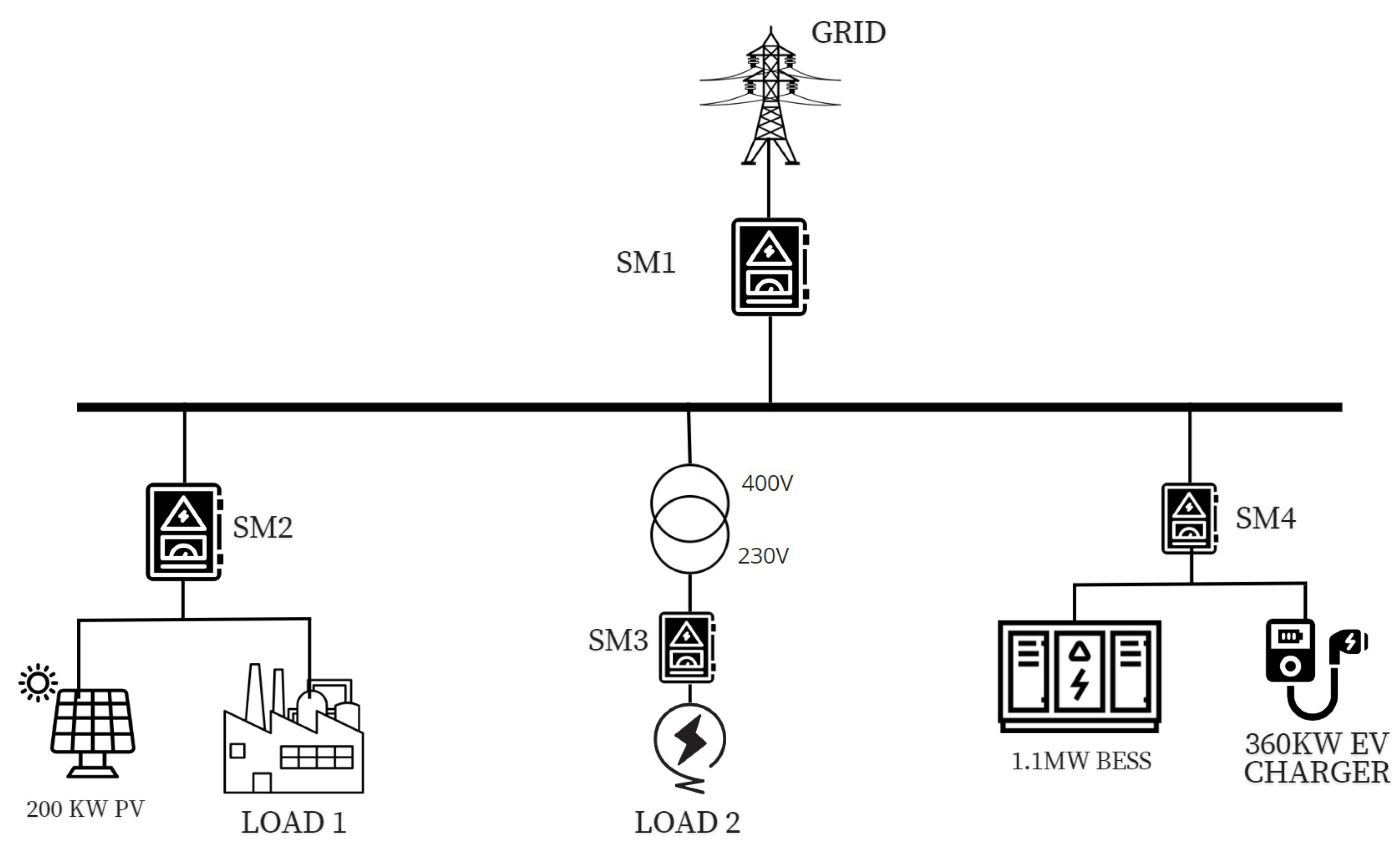
Figure 2.
Forecasted PV Power Generation throughout 2024.
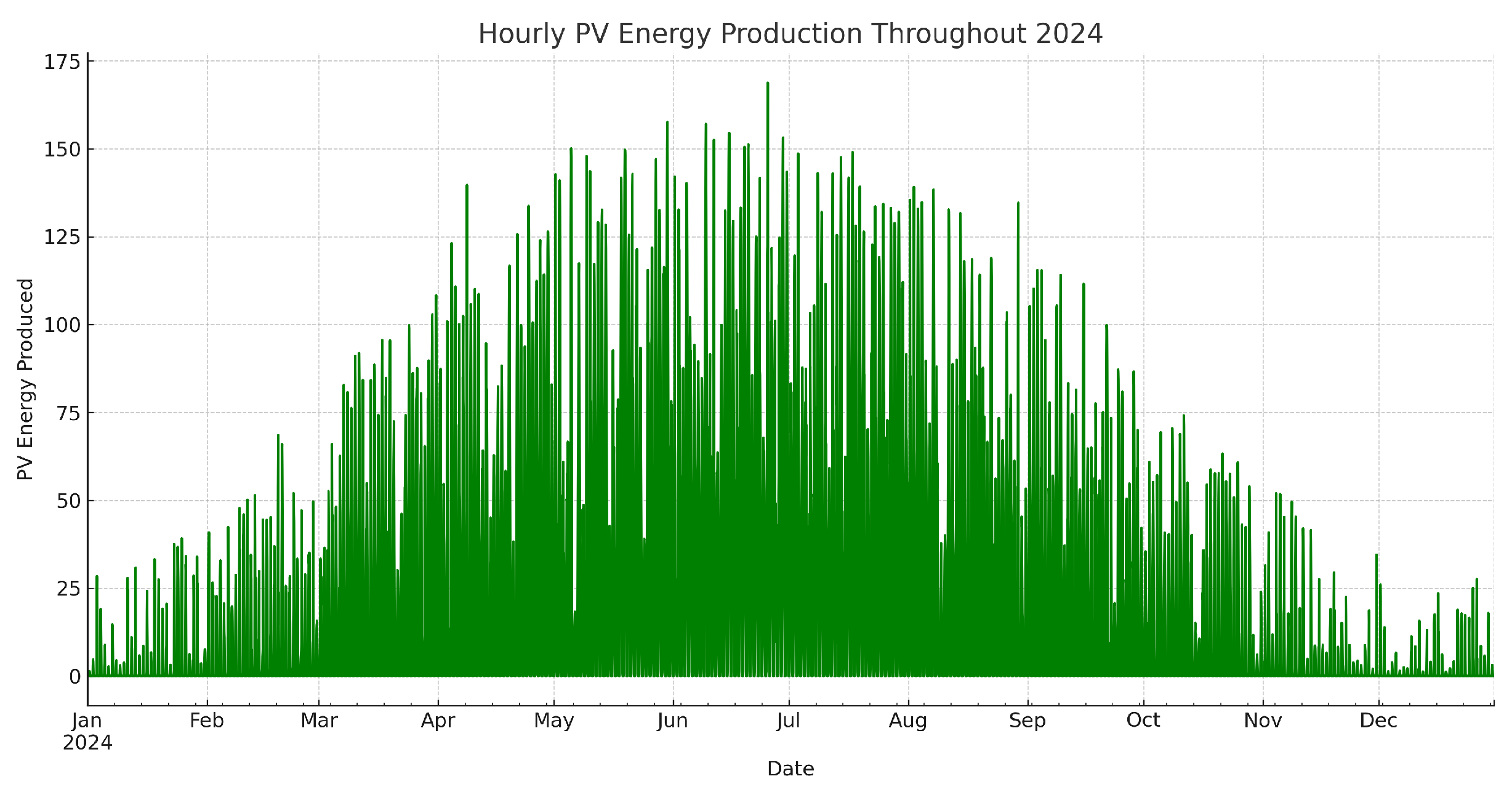
Figure 3.
Overview of the Energy Management System.
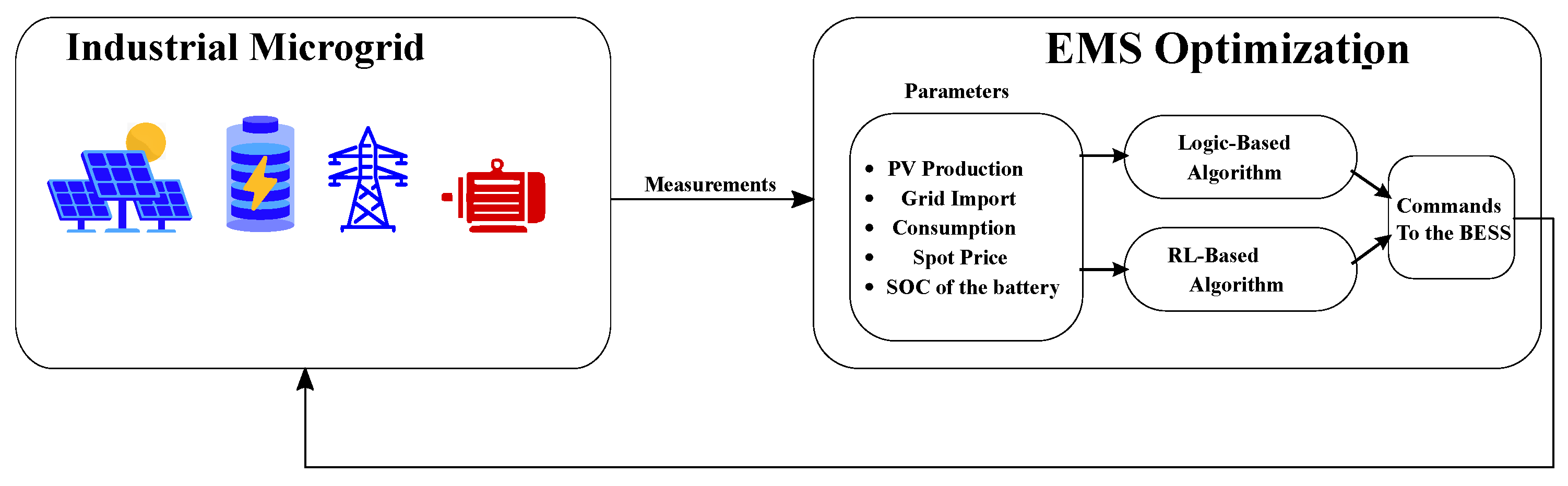
Figure 4.
EMS Development Steps.
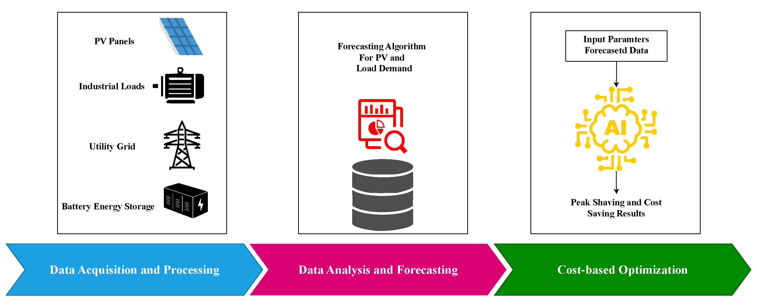
Figure 5.
Forecasted Graph of Grid Import and Site Load.
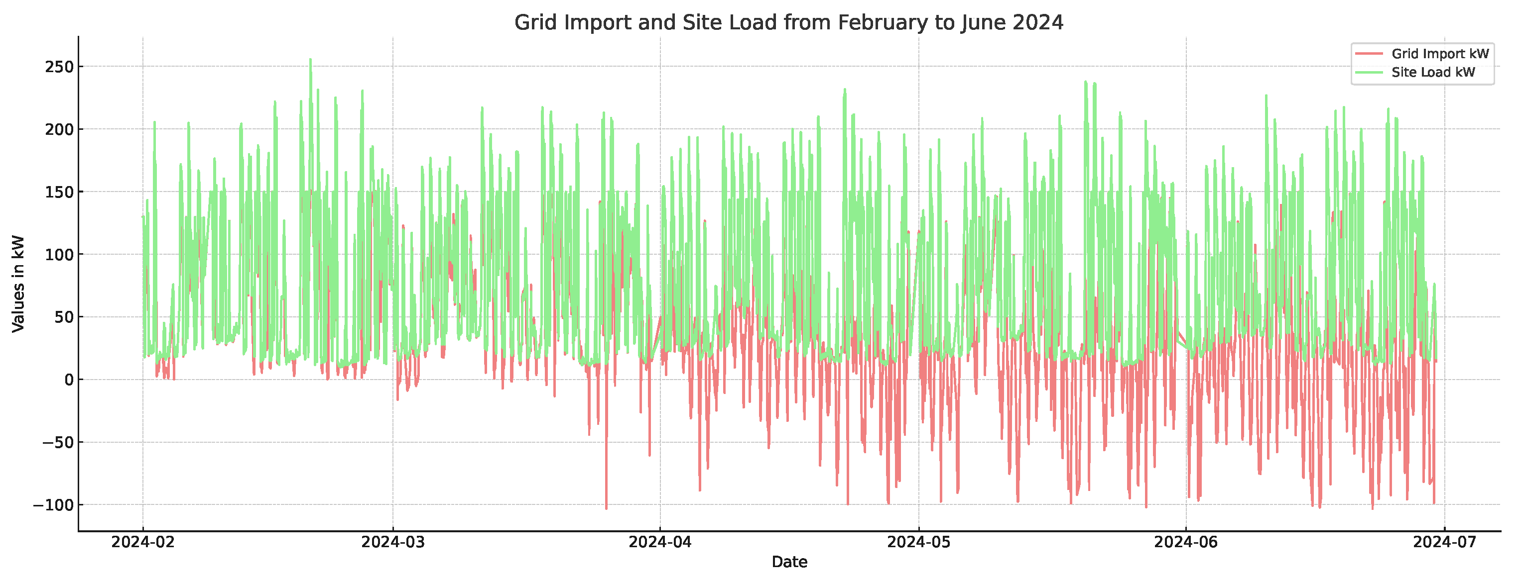
Figure 6.
Flowchart of the Logic-Based Optimization Algorithm.
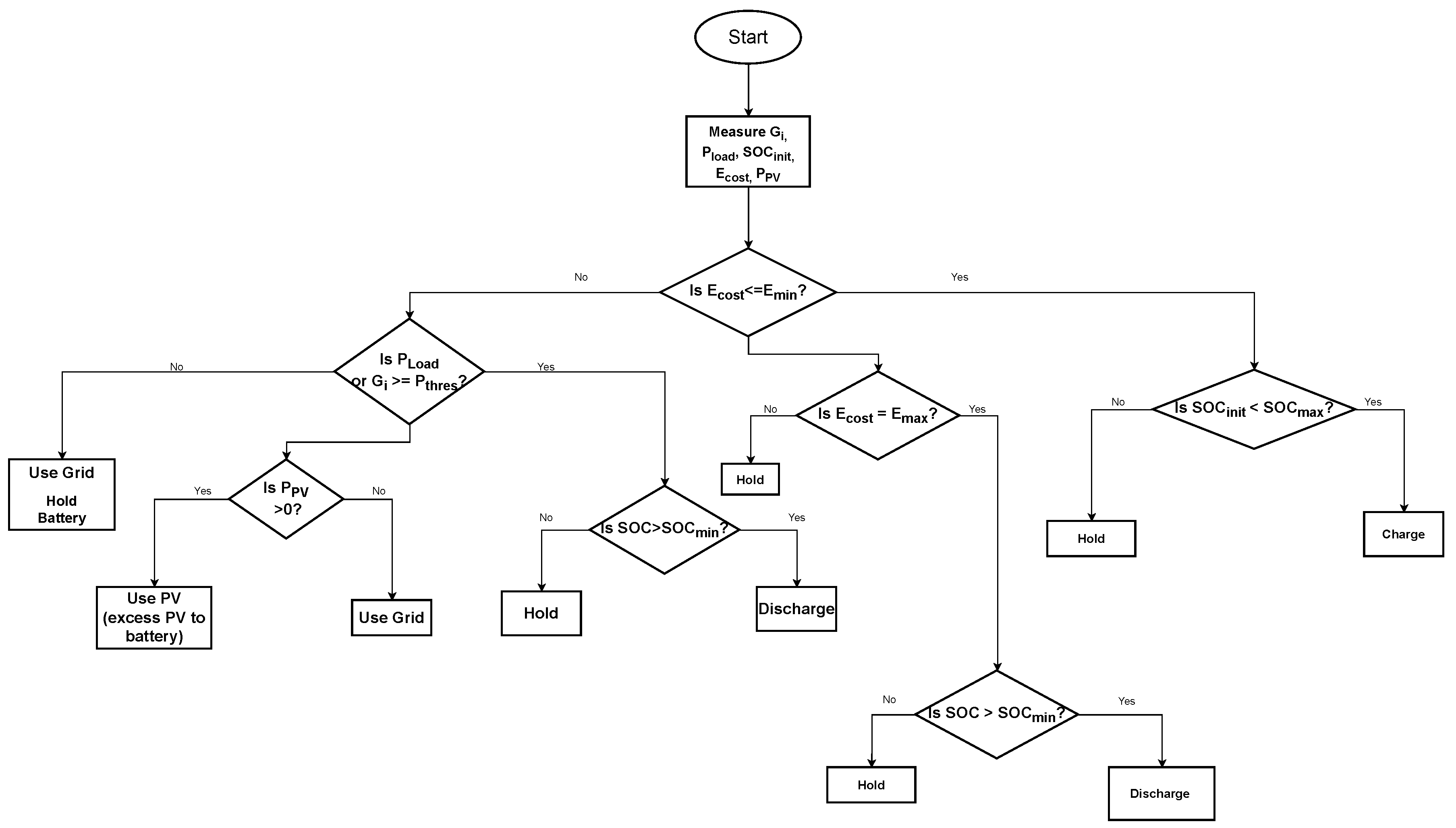
Figure 7.
Workflow of PPO algorithm.
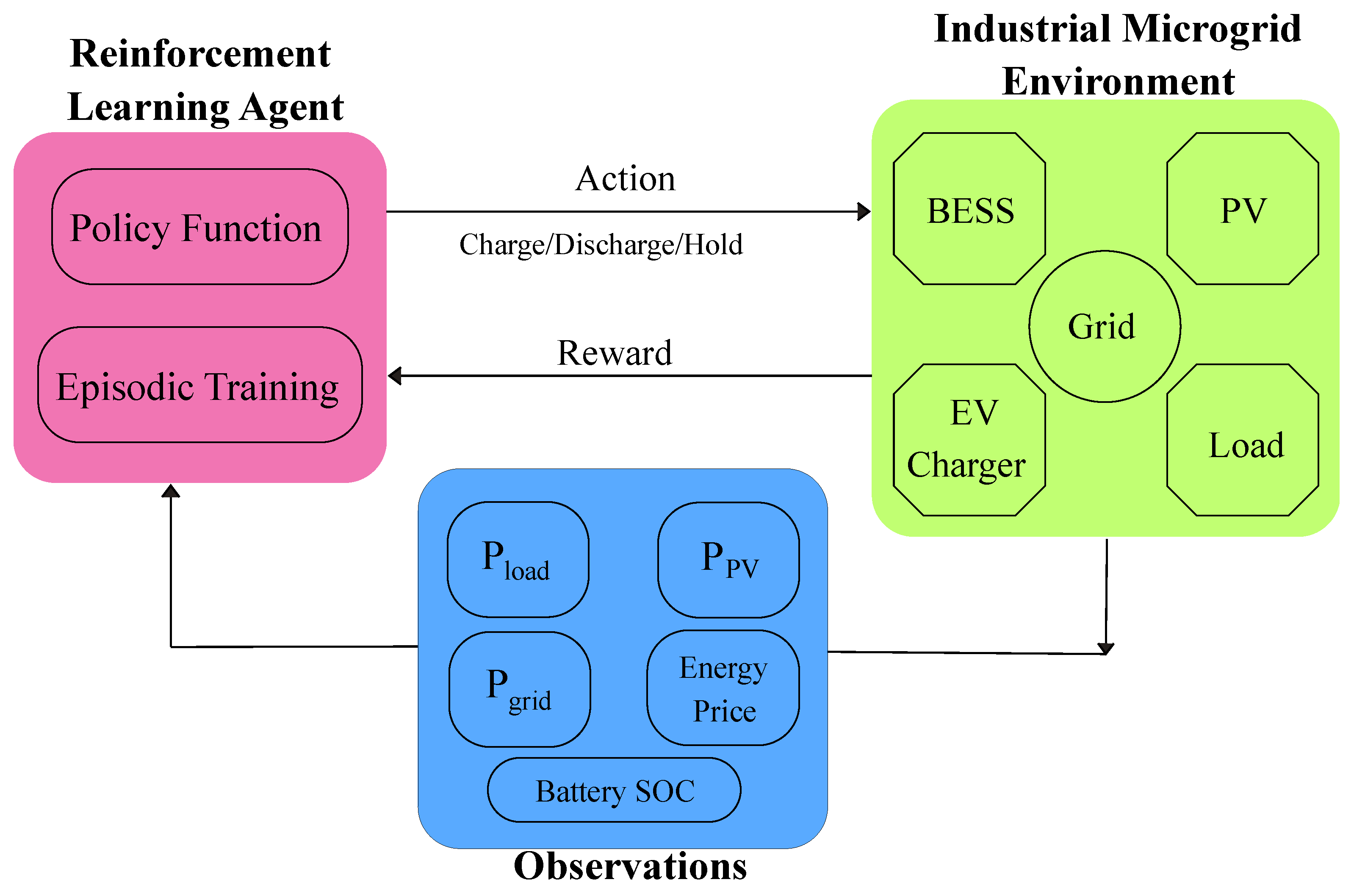
Figure 8.
Grid import, site load, energy price, battery power, and SOC for a day in July.
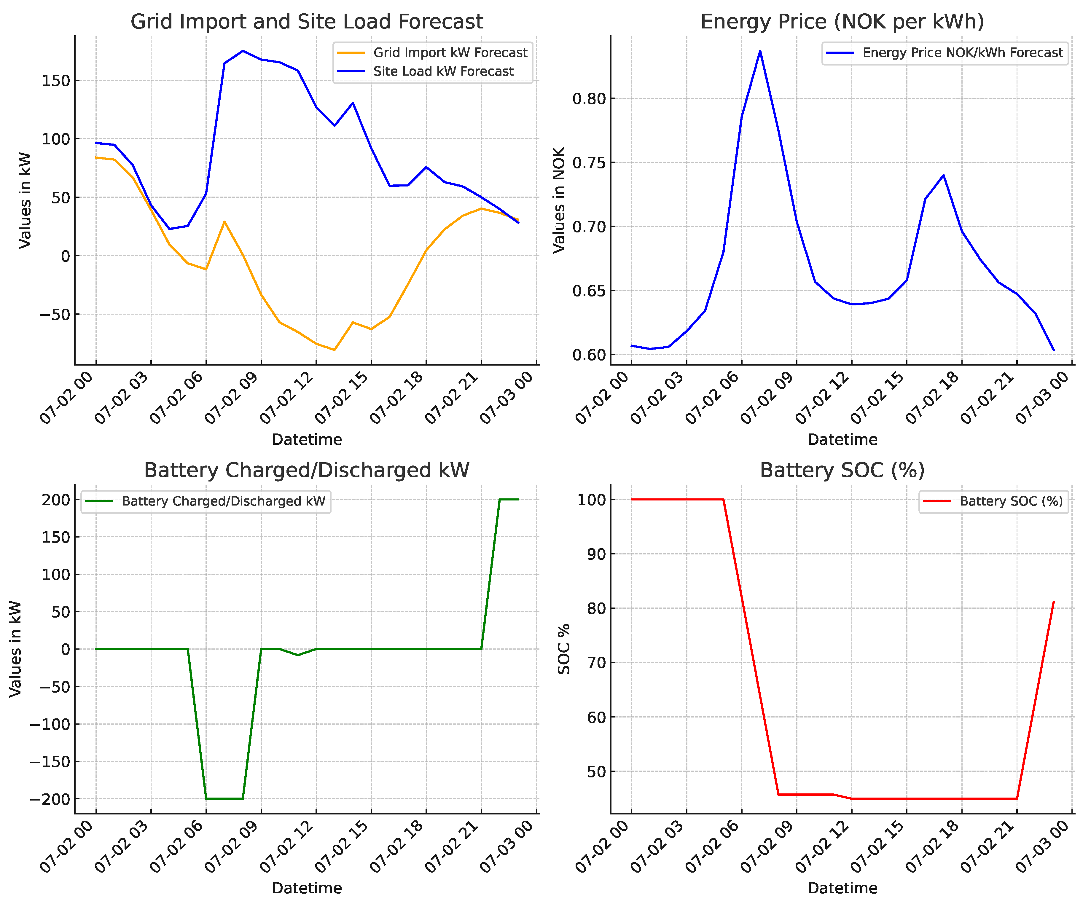
Figure 9.
Monthly Cost Savings using the Logic-based Optimization Algorithm.
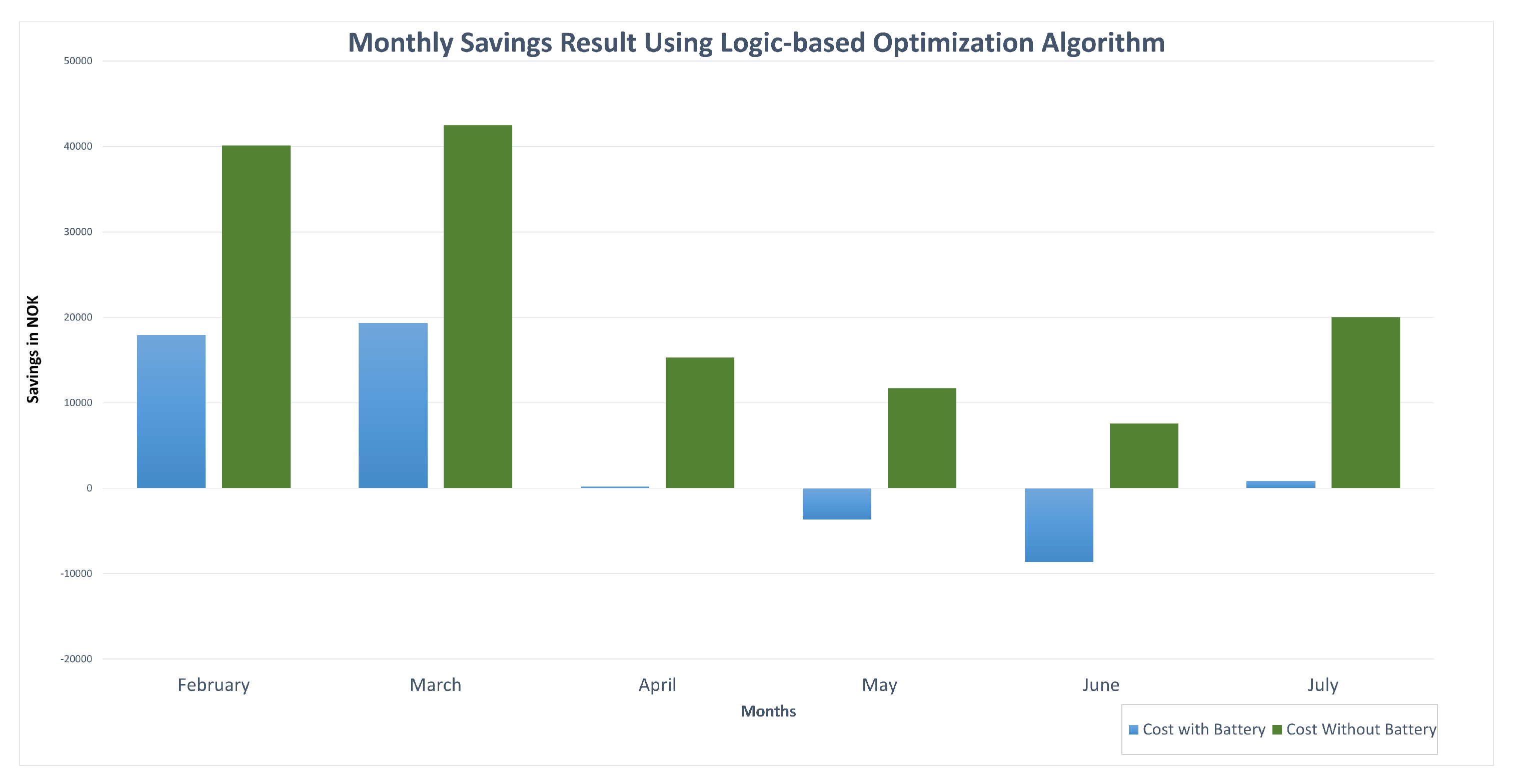
Figure 10.
Monthly Savings Results from the RL Algorithm.
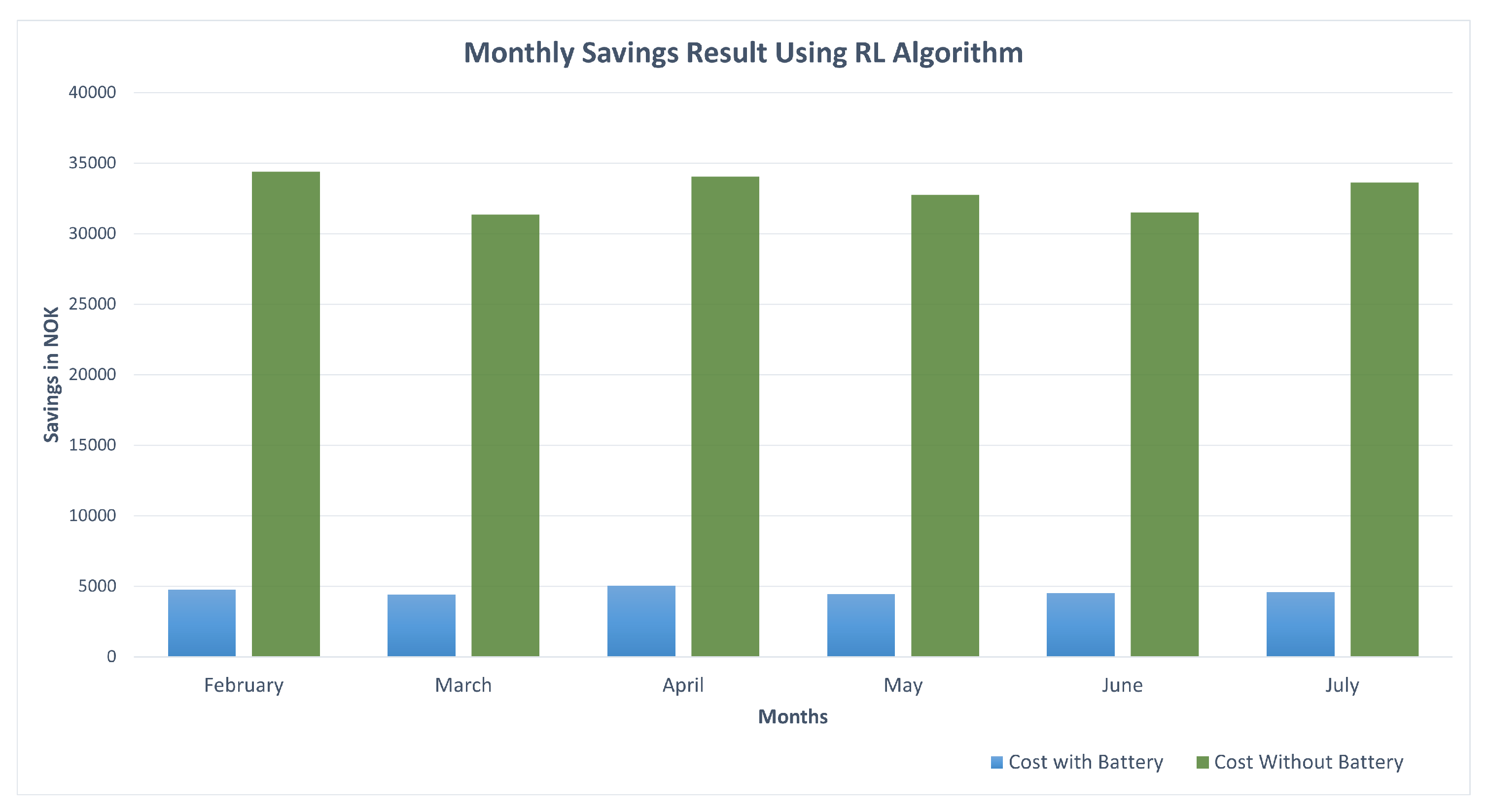
Figure 11.
Monthly Savings Results Comparision from both Algorithms.
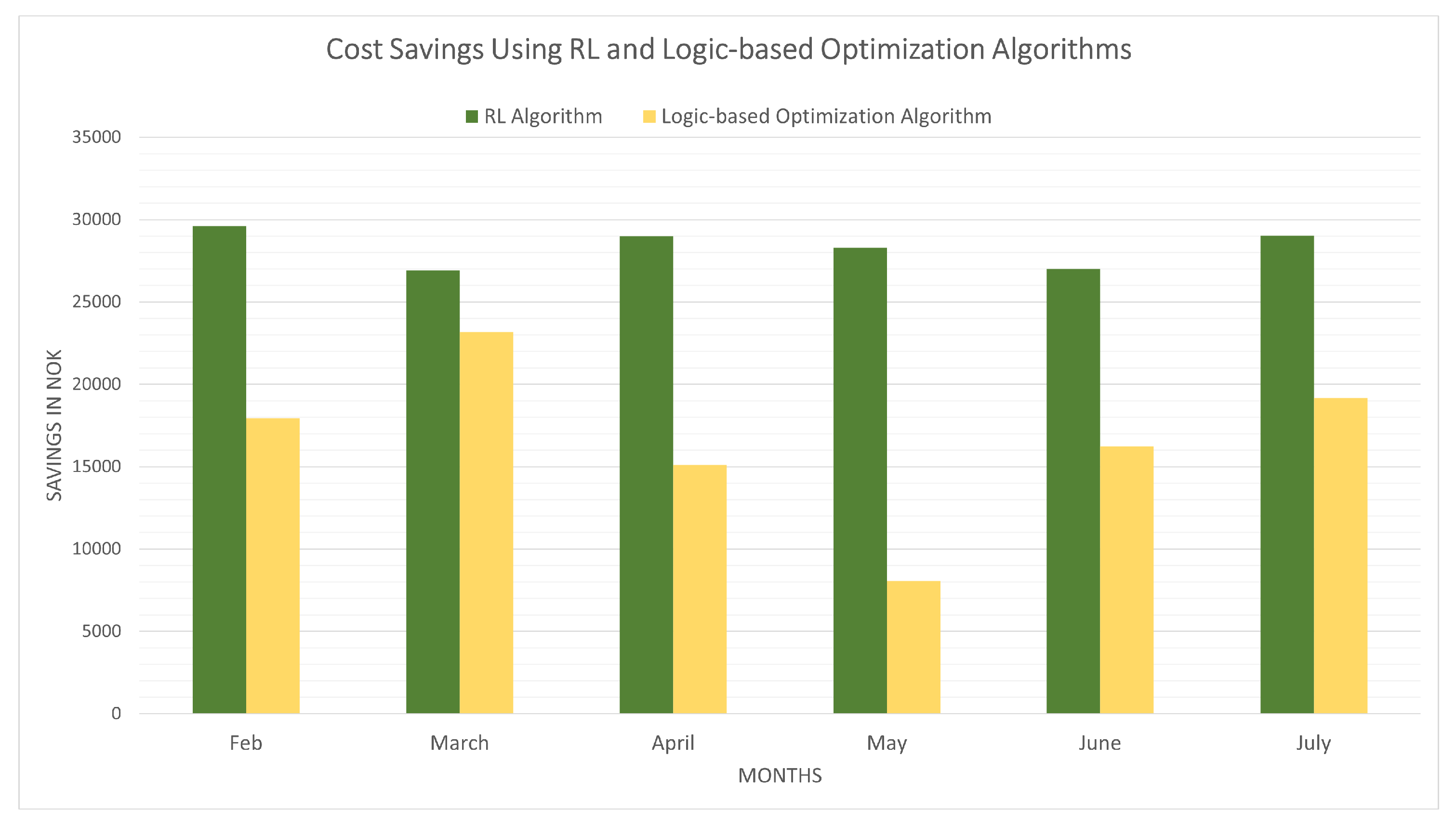
Figure 12.
Normalized results for the spot price, SOC, and battery.
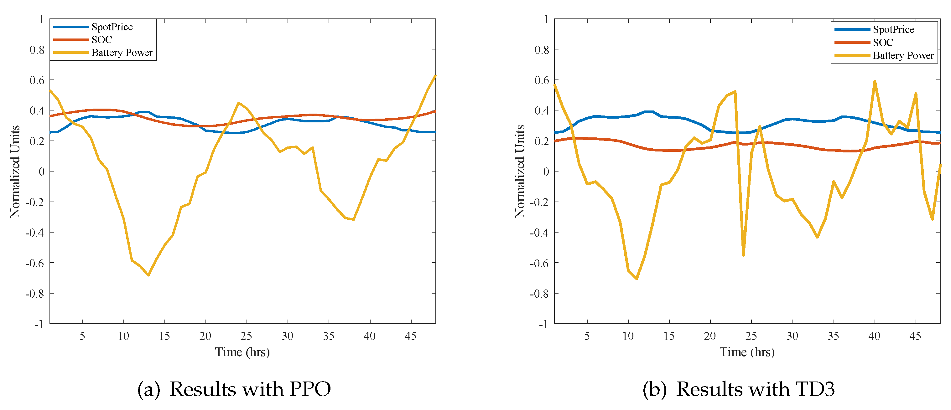
Figure 13.
Comparison of the , electricity cost, , and the SOC between TD3 and PPO.
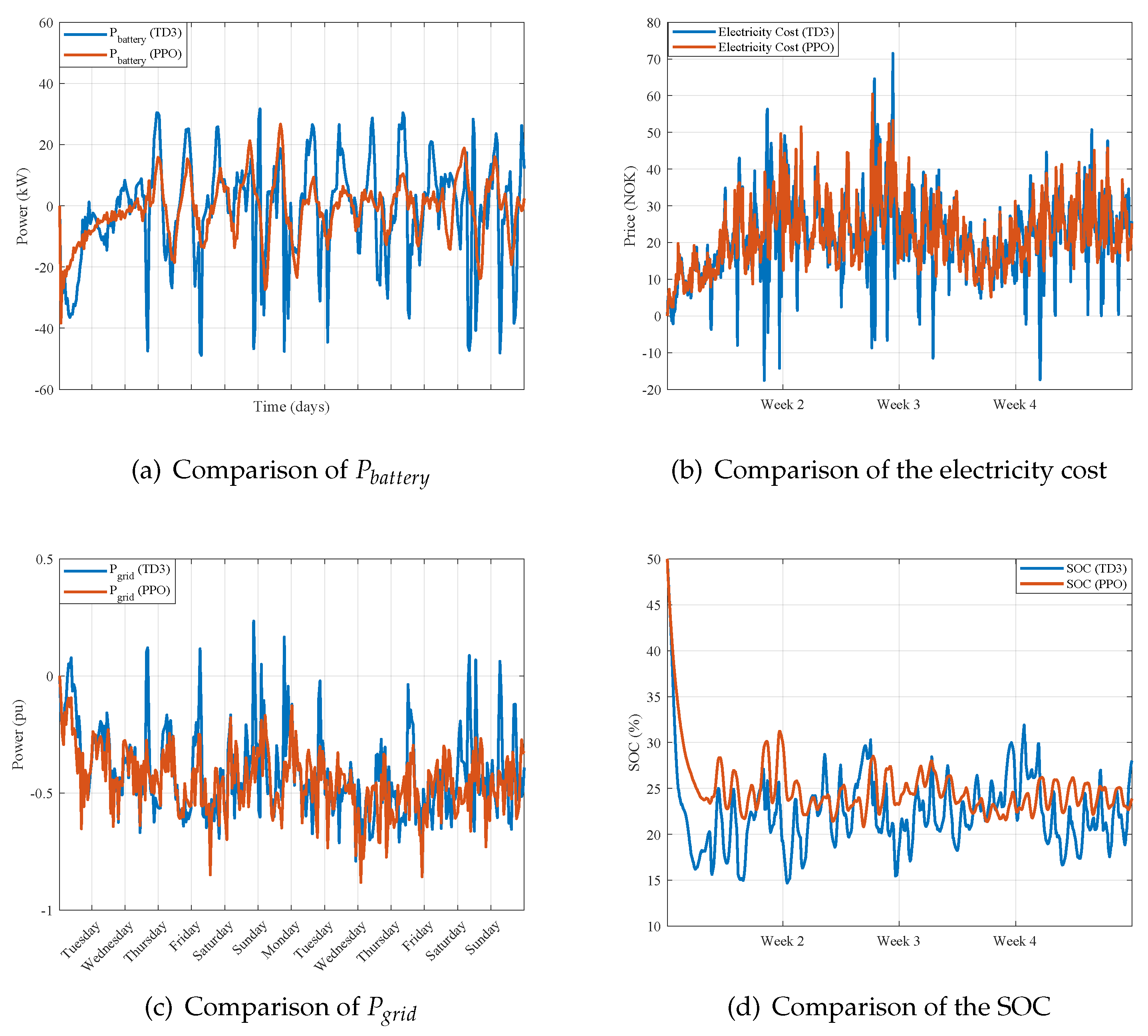
Table 1.
General PV System Parameters.
| Parameters | Values |
|---|---|
| PV Generator Output | 200.88 kWp |
| PV Generator Surface | 1059.6 m2 |
| Number of PV Modules | 648 |
| Number of Inverters | 3 |
| PV Module Used | JAM60S01-310/PR |
| Speculated Annual Yield | 87,594 kWh/kWp |
Table 2.
Table showing Battery System Specifications.
| Parameters | Values |
|---|---|
| Battery Type | LPF Lithium-ion |
| Battery Capacity | 1105 kWh |
| Rated Battery Voltage | 768 Vdc |
| Battery Voltage Range | 672-852 Vdc |
| Max. Charge/Discharge Current | 186 A |
| Max. Charge/Discharge Power | 1000 kW |
Table 4.
Summary of the mcirogrid peak hour pricing scheme.
| Peak hour pricing scheme (taken from the highest peak in the month) |
| Winter: From November - March (84 kr/kW/month) |
| Summer: From April - October (35 kr/kW/month) |
| Peak hour pricing scheme for reactive power (taken from the highest peak in the month) |
| Winter: From November - March (35 kr/kVAr/month) |
| Summer: From April - October (15 kr/kW/month) |
Disclaimer/Publisher’s Note: The statements, opinions and data contained in all publications are solely those of the individual author(s) and contributor(s) and not of MDPI and/or the editor(s). MDPI and/or the editor(s) disclaim responsibility for any injury to people or property resulting from any ideas, methods, instructions or products referred to in the content. |
© 2024 by the authors. Licensee MDPI, Basel, Switzerland. This article is an open access article distributed under the terms and conditions of the Creative Commons Attribution (CC BY) license (http://creativecommons.org/licenses/by/4.0/).
Copyright: This open access article is published under a Creative Commons CC BY 4.0 license, which permit the free download, distribution, and reuse, provided that the author and preprint are cited in any reuse.


