Submitted:
05 February 2026
Posted:
13 February 2026
You are already at the latest version
Abstract
Type Ia supernovae (SNe Ia) are luminous thermonuclear transients whose peak luminosities can be standardized, enabling measurements of luminosity distance over cosmological redshifts and an empirical Hubble diagram of distance modulus versus redshift that constrains the distance–redshift relation. Direct empirical tests in which redshift-dependent scalings of fundamental constants are applied to SN Ia distances remain scarce relative to fixed-constant interpretations. The aim is to determine whether a one-parameter unified-flow scaling of the distance scale can reproduce the Pantheon+SH0ES SN Ia Hubble diagram without introducing an explicit dark-energy term, and to quantify the resulting constraint on the scaling exponent. The model treats redshift evolution as a single coherent scaling that links the effective gravitational coupling and the light-propagation scale in a reciprocal manner, yielding an analytic luminosity-distance prediction under a matter-closure expansion law. The scaling exponent is estimated from Pantheon+SH0ES (1701 SNe Ia spanning redshifts 0.00122 to 2.26137) using the full statistical and systematic covariance matrix and an exact analytic profiling of the distance-modulus offset. The best fit is an exponent of negative 0.4975 (68% profile interval from negative 0.5165 to negative 0.4785) with a minimum chi-squared of 1751.82 for 1699 degrees of freedom; the fixed-constants matter-only baseline is disfavored by a chi-squared difference of 640.20, while a supernova-only flat Lambda CDM benchmark gives a matter density parameter of 0.3612 with an uncertainty of 0.0187 and a minimum chi-squared of 1752.51. After profiling the distance-modulus offset, the unified-flow and Lambda CDM distance laws differ by about 0.259 magnitudes at redshift 2.26137 and separate further at higher redshift. These results provide an empirically constrained, covariance-respecting phenomenological distance law consistent with current SN Ia distances and yield a falsifiable prediction for future higher-redshift standard candles or standard sirens.
Keywords:
type Ia supernovae
; Pantheon+SH0ES
; luminosity distance
; varying constants
; covariance matrix
; Cholesky whitening
; profile likelihood
; Akaike information criterion
; Λ CDM
1. Introduction
Type Ia supernovae (SNe Ia) are luminous transients widely interpreted as thermonuclear disruptions of carbon–oxygen white dwarfs in binary systems. Their spectra and light-curve morphologies form a comparatively homogeneous class, and empirical correlations between peak brightness, post-maximum decline rate, and color enable their use as standardizable candles for distance determination [1,2,3,4,5]. For each object, a standardized distance modulus provides an estimate of the luminosity distance , up to an overall calibration offset that absorbs the absolute magnitude and the present-day distance scale.
A SN Ia Hubble diagram is the empirical relation between standardized distance moduli and redshift. In practice, the Hubble diagram is constructed by plotting (or equivalent magnitude residuals) against a spectroscopic redshift corrected to an appropriate cosmological frame, and comparing the resulting distance–redshift trend to model predictions for . Because depends on the line-of-sight integral of the light-propagation scale in homogeneous kinematics, the Hubble diagram probes the shape of the distance law and its redshift dependence. Early Hubble-diagram extensions to more distant SNe Ia [6] and subsequent studies have investigated potential systematics and wavelength dependence, including host-galaxy correlations [7] and near-infrared Hubble diagrams with reduced sensitivity to dust [8,9]. High-redshift Hubble diagrams provided the first direct evidence that the observed distances depart from a simple fixed-constant, matter-only prediction, motivating models that introduce a cosmological constant or other late-time component [10,11,12].
Although these phenomenological extensions describe a broad set of observations, the microphysical origin of an effective late-time acceleration remains uncertain, and the cosmological constant problem continues to motivate empirical tests of alternative distance–redshift parameterizations [13,14]. In this context, modifications that act directly on the distance scale—rather than on an explicit energy component—provide a complementary way to interrogate the information encoded in the SN Hubble diagram alone.
Redshift dependence of effective couplings is one class of such modifications. Theoretical motivations and phenomenological frameworks include scalar–tensor gravity [15], varying-speed-of-light (VSL) proposals [16,17,18,19], and broader observational reviews emphasizing that physical interpretation must ultimately be cast in terms of dimensionless quantities [20,21]. Even when interpreted purely as an effective ansatz, redshift-dependent scalings modify the combination that determines , and therefore admit direct confrontation with Hubble-diagram distances. Despite the extensive literature on varying-constant ideas, empirical, covariance-respecting fits that apply a redshift-dependent scaling directly to SN Ia distance moduli remain limited.
A one-parameter unified-flow distance law is therefore tested against the Pantheon+SH0ES compilation. The model encodes an effective redshift dependence through a single exponent in , adopts a matter-closure scaling for , and yields an analytic expression for the dimensionless luminosity distance. The parameter is estimated using the full Pantheon+SH0ES statistical+systematic covariance matrix with an exact analytic profiling of the distance-modulus offset, and the resulting fit is compared to a fixed-constants matter-only baseline and to a supernova-only flat CDM benchmark.
2. Materials and Methods
2.1. Data
The analysis uses SNe Ia from the Pantheon+SH0ES data products released with Pantheon+ [22]. The subset is labeled “Pantheon+SH0ES” because it overlaps the Cepheid-calibrated supernova sample employed by SH0ES in the distance-ladder analysis [23]. The Hubble-diagram redshift supplied with the data products, , is adopted throughout, giving , together with the corresponding observed distance moduli (column MU_SH0ES in the release files). The full covariance matrix supplied with the data products (statistical and systematic components) is used without approximation.
2.2. Unified-Flow Factor and Redshift Scalings
A single flow factor
where z is redshift. The flow factor parameterizes redshift dependence of the effective constants through the canonical scalings
where subscript “0” denotes the reference values. Here denotes an effective gravitational coupling, an effective light-propagation scale, and an effective proper-time interval; , , and denote the corresponding reference values. The exponent is assumed constant across the dataset (i.e., a single parameter describing the full redshift range of Pantheon+SH0ES) and is not promoted to a function in this formulation.
In this supernova-only application, Equation (2) is treated as an effective scaling ansatz: the Hubble-diagram fit depends only on the derived combination that enters the luminosity-distance integral (Equation (5)), while a complete dynamical theory would be required to connect to the evolution of dimensionless couplings and to local tests.
2.3. Background Expansion and Luminosity Distance
A matter-dominated background with the Friedmann scaling (where is the matter density) and implies
In Equation (3), is the Hubble expansion rate at redshift z and is its value at . Combining Equations (2) and (3) yields a power-law form for the light-travel factor
Assuming spatial flatness for the purpose of the distance integral, the luminosity distance can be written as
where is a dummy integration variable. The overall scale is degenerate with the SN absolute magnitude and is absorbed into the offset parameter M (Section 2.5). A dimensionless distance proxy is defined by factoring out :
Evaluating Equation (5) gives the closed form
with .
2.3.1. Continuity and Baseline Reduction Checks
Two identities are required for mathematical continuity and for verification of limiting behavior.
Baseline reduction ().
At , Equation (7) must reproduce the matter-only baseline
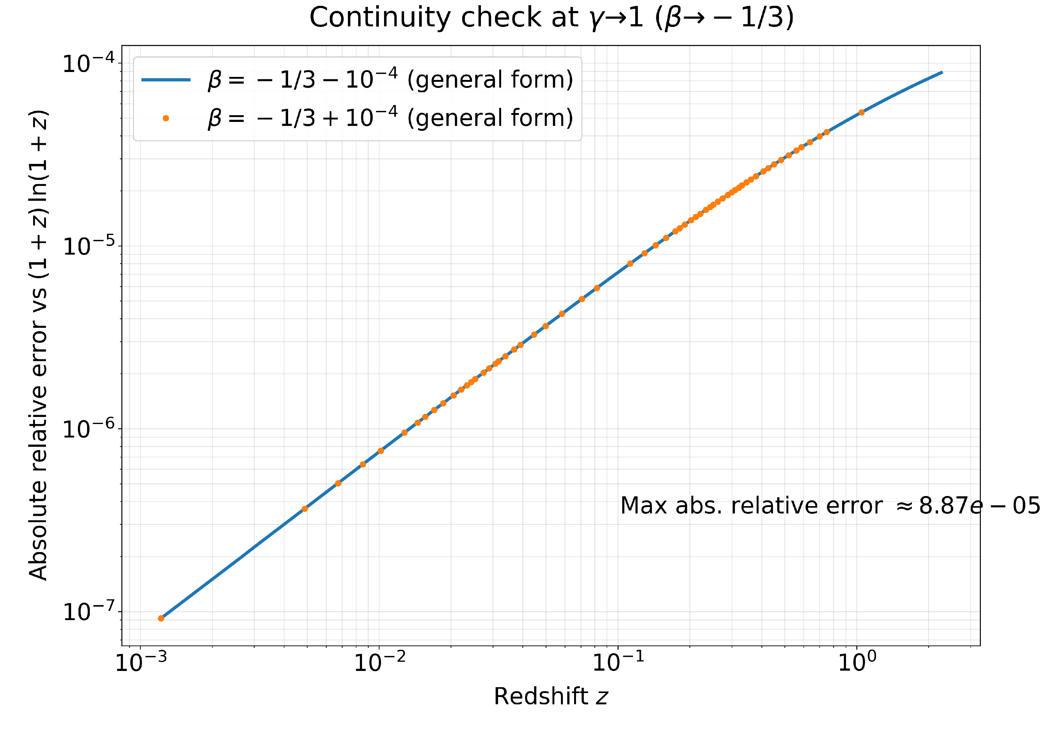
Continuous limit at ().
The form in Equation (7) must approach as , ensuring continuity at .
The numerical verification of these identities (Figures 7 and 8) is reported in Section 2.9.
2.4. Distance Modulus Model
The theoretical distance modulus is defined as
where M is a nuisance offset absorbing the absolute magnitude calibration and the overall distance normalization (Equation (6)).
2.5. Likelihood, Covariance Weighting, and Analytic Profiling of M
Assuming a multivariate normal likelihood with covariance , the chi-squared function is
A Cholesky factorization is used to avoid explicit matrix inversion. Defining the residual vector
where and is the N-vector of ones, the chi-squared becomes
Because M enters linearly, it is profiled out analytically at each . Defining and and , the profiled offset is
Substituting into Equation (12) yields the profile chi-squared .
2.6. Parameter Estimation, Confidence Intervals, and Model Comparison
The best-fit exponent minimizes the profile chi-squared . Profile-likelihood intervals for a single parameter use
with thresholds (68% confidence) and (95% confidence) [24].
Model comparison between the unified-flow model (free ) and the fixed-constants baseline () uses the likelihood-ratio statistic and the Akaike information criterion (AIC) [25,26]:
where k is the number of fitted parameters ( for and for at ).
For completeness, the Bayesian information criterion (BIC) is also reported:
2.7. Residual Diagnostics and Goodness-of-Fit Tests
Whitened residuals are defined by
A covariance-weighted root-mean-square statistic is reported as
To assess possible redshift-dependent structure in the marginal residual distribution, a two-sample Kolmogorov–Smirnov (KS) statistic is computed for the unwhitened residuals after splitting the sample at ; the associated p-value is reported as a descriptive diagnostic [27].
2.8. Low-Redshift Sensitivity Bound (no Low-z-Only Fit)
The exponent affects only beyond the linear Hubble-law term. Expanding Equation (7) for gives
so that the corresponding distance modulus satisfies
Because the nuisance offset M is fitted simultaneously, the effective sensitivity to in a low-z subsample is further reduced by partial degeneracy with the intercept.
Let the parameter vector be . Under the Gaussian likelihood of Equation (10), the Fisher matrix for a subset with covariance is
Profiling over the linear offset M yields an effective Fisher information for ,
For the 500 lowest-redshift objects in Pantheon+SH0ES (), evaluation with the supplied covariance submatrix gives , consistent with weak constraining power from this redshift range once the intercept is profiled. Accordingly, no low-z-only best-fit is reported, and the full-sample inference is adopted as the definitive constraint within the assumed constant- model.
2.9. Numerical Verification of Limiting Cases
Two numerical checks validate the implementation of Equation (7). Figure 7 reports the absolute relative error between Equation (7) evaluated at and the baseline expression in Equation (8). Figure 8 reports the absolute relative error between the form near and the logarithmic limit, validating continuity.
3. Results
3.1. Best-Fit Parameters and Goodness of Fit
The unified-flow model provides an excellent match to the Pantheon+SH0ES Hubble diagram (Figure 1). Minimization of the profiled chi-squared yields
The minimum chi-squared is for , giving (Table 1).
3.2. Comparison to the Fixed-Constants Baseline
3.3. Residual diagnostics
Figure 2 displays residuals versus redshift with a split marker at . A two-sample KS statistic computed on the marginal residual distributions for and yields (Table 2), providing no evidence for a pronounced change in the residual distribution across this split. The covariance-weighted WRMS (Equation (18)) is close to unity (Table 2).
Figure 2.
Residuals versus redshift. The vertical dashed line marks the diagnostic split at used for the KS test. The redshift axis is logarithmic.
Figure 2.
Residuals versus redshift. The vertical dashed line marks the diagnostic split at used for the KS test. The redshift axis is logarithmic.
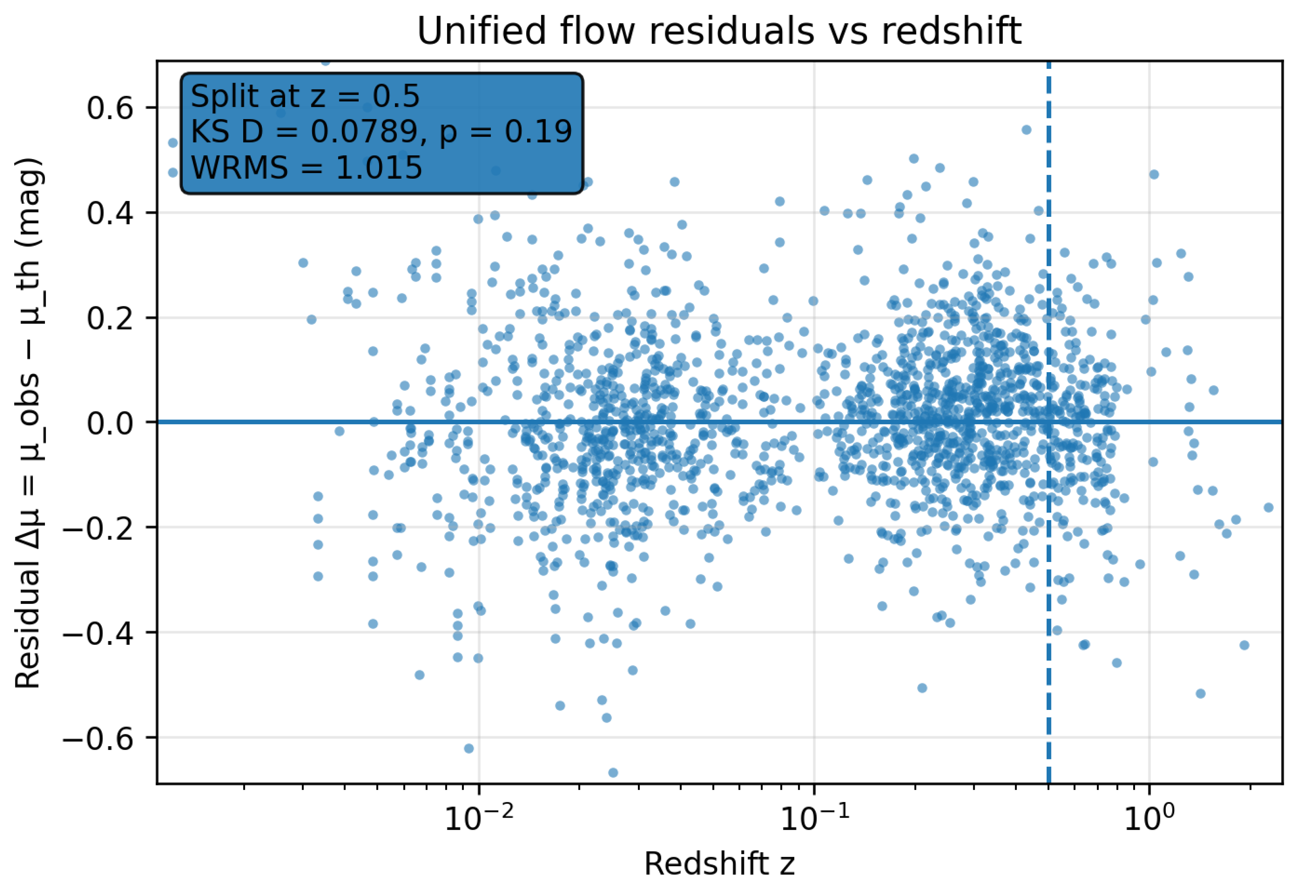
Figure 3.
Residual distributions for and corresponding to the diagnostic split. The Kolmogorov–Smirnov statistic and p-value for this split are reported in Table 2.
Figure 3.
Residual distributions for and corresponding to the diagnostic split. The Kolmogorov–Smirnov statistic and p-value for this split are reported in Table 2.
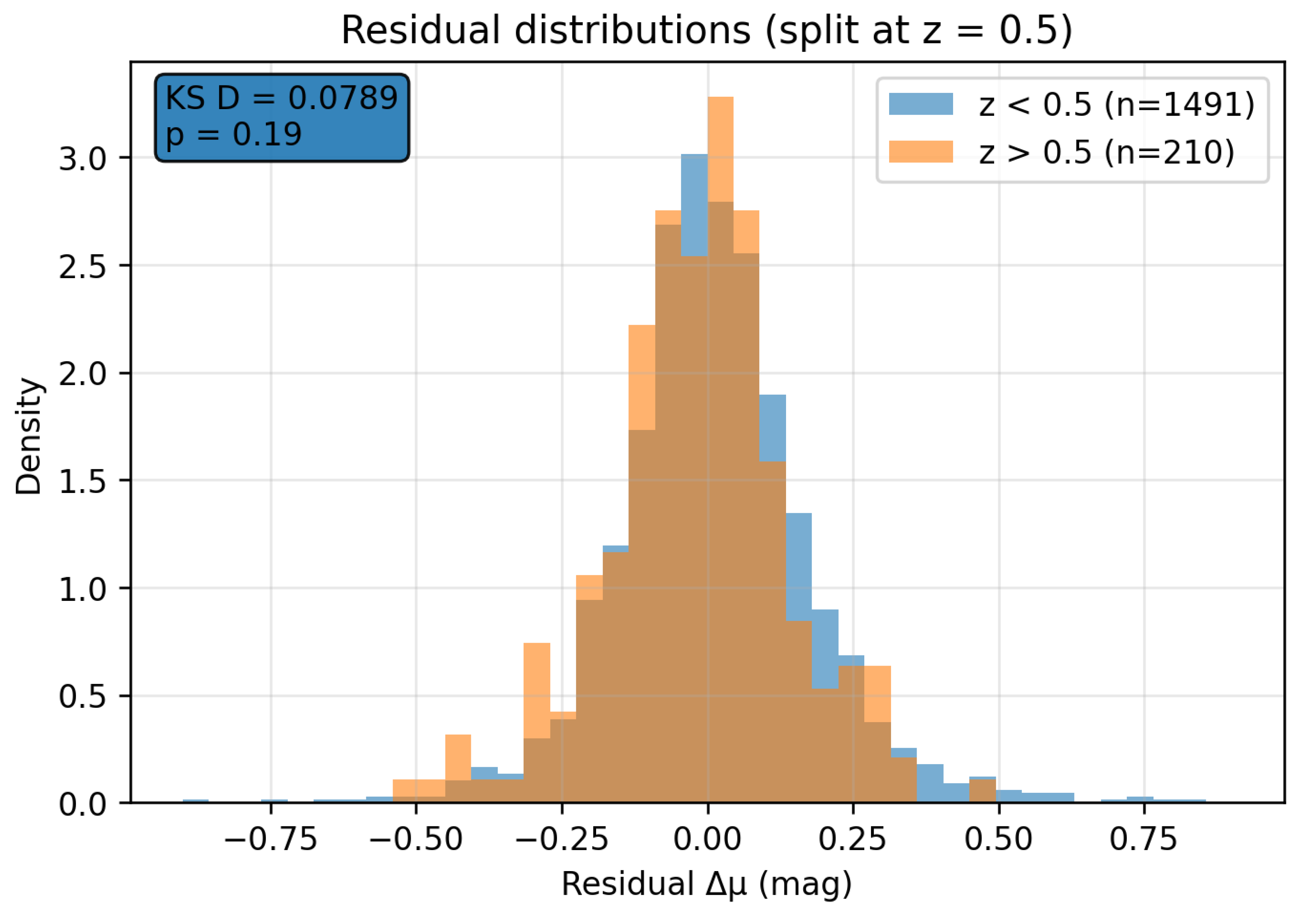
Figure 4.
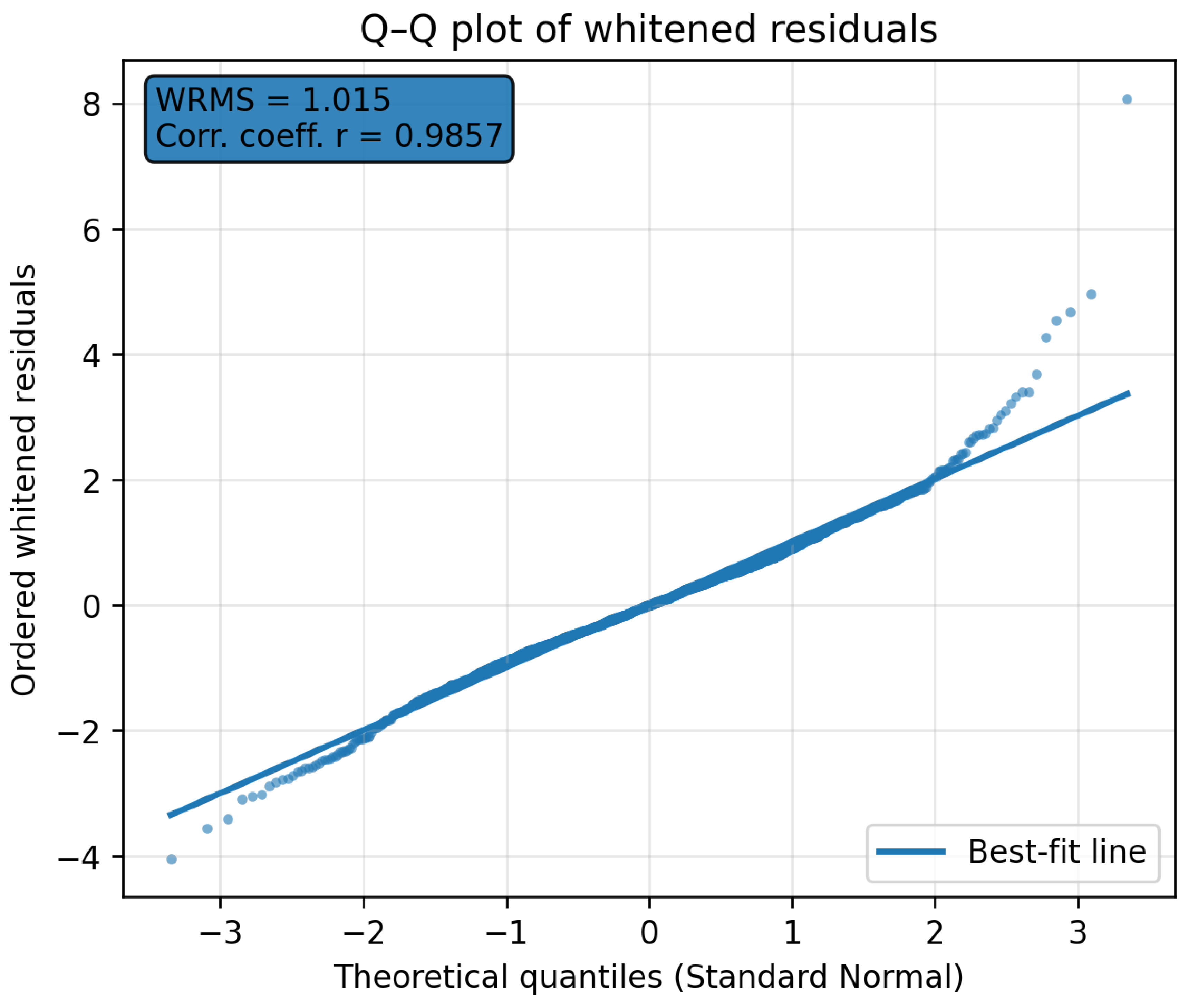
Q–Q plot of the whitened residuals (Equation (17)) against standard-normal quantiles. The near-linear trend and WRMS close to unity support proper covariance weighting.
Figure 4.
Q–Q plot of the whitened residuals (Equation (17)) against standard-normal quantiles. The near-linear trend and WRMS close to unity support proper covariance weighting.
3.4. Profile Likelihood for and Confidence Intervals
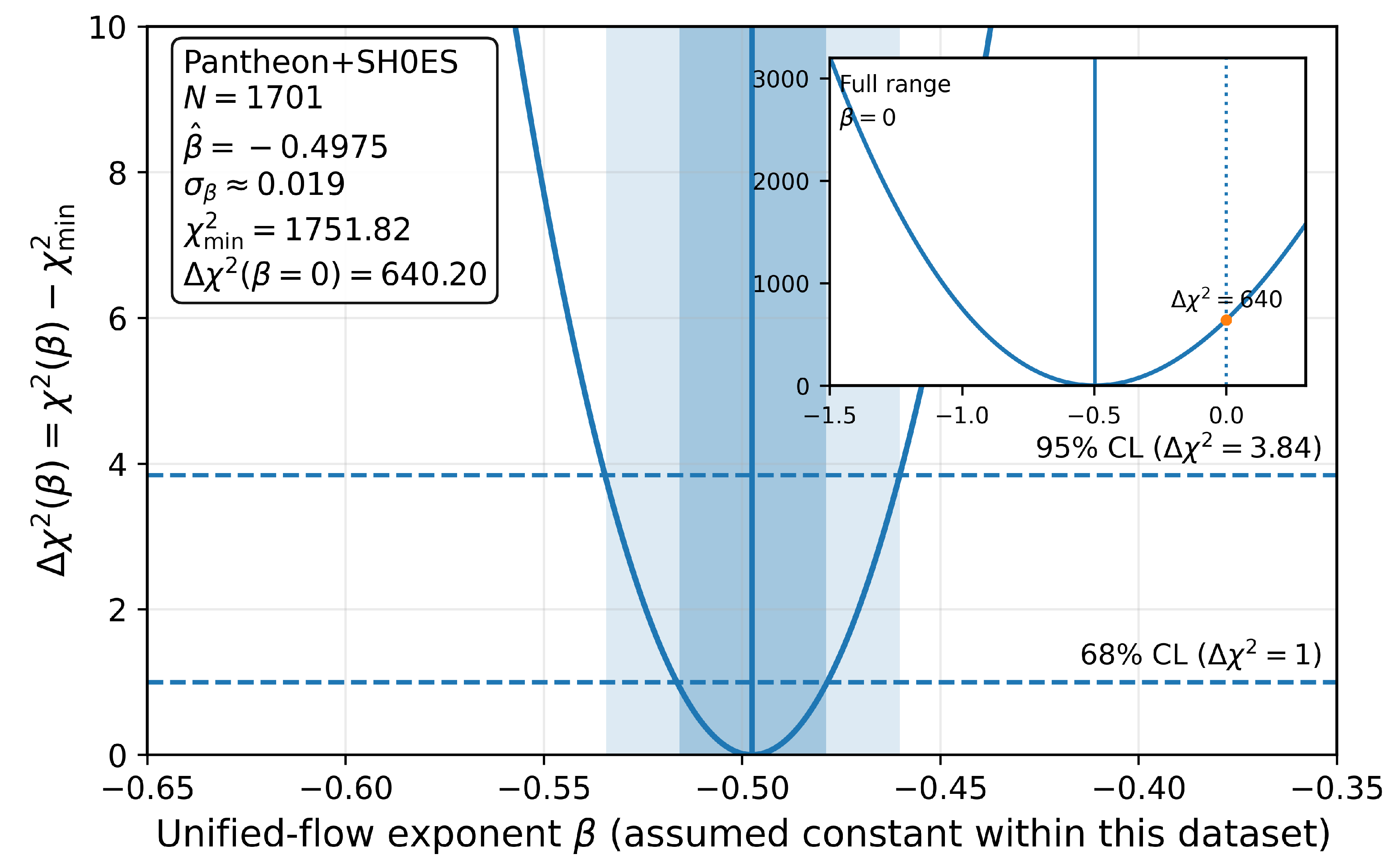
The profile likelihood is shown in Figure 5. One-parameter confidence intervals derived from the profile likelihood are summarized in Table 3.
Figure 5.
Profile likelihood for the unified-flow exponent computed as . The shaded regions indicate the 68% and 95% confidence intervals for one parameter ( and ).
Figure 5.
Profile likelihood for the unified-flow exponent computed as . The shaded regions indicate the 68% and 95% confidence intervals for one parameter ( and ).
3.5. Profiled Nuisance Parameter
The nuisance offset profiled by Equation (13) varies smoothly with (Figure 6), with at the best-fit exponent.
Figure 6.
Profiled nuisance parameter obtained from Equation (13). The dashed line marks at the best-fit .
Figure 6.
Profiled nuisance parameter obtained from Equation (13). The dashed line marks at the best-fit .
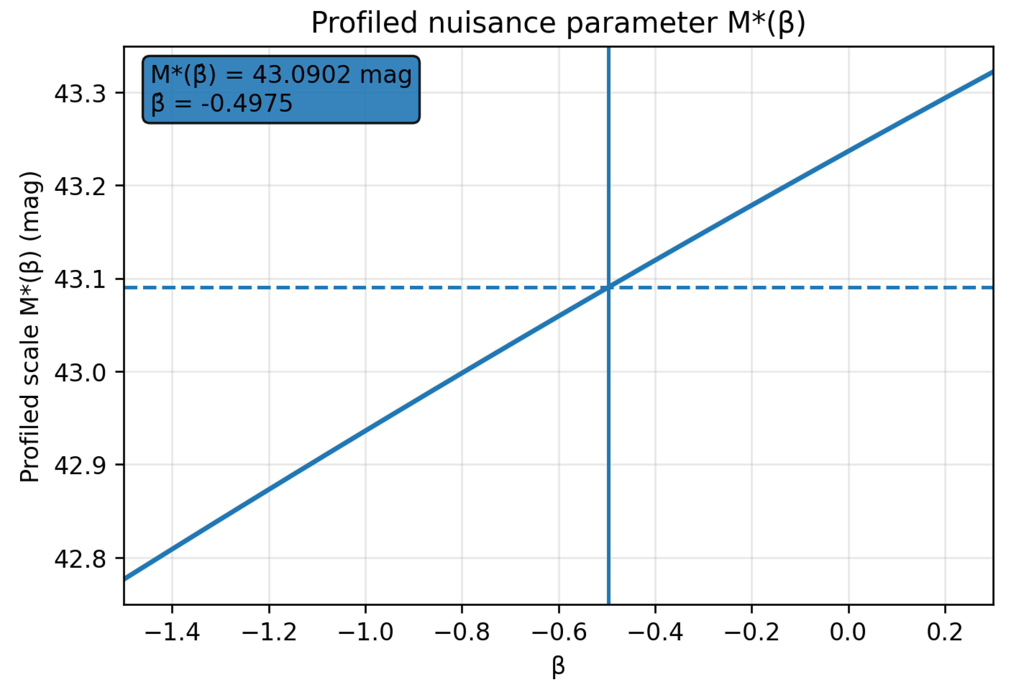
Figure 7.
Verification of the baseline reduction identity at : absolute relative error between the general closed form (Equation (7)) and the matter-only baseline (Equation (8)) across the dataset redshifts. The redshift and error axes are logarithmic.
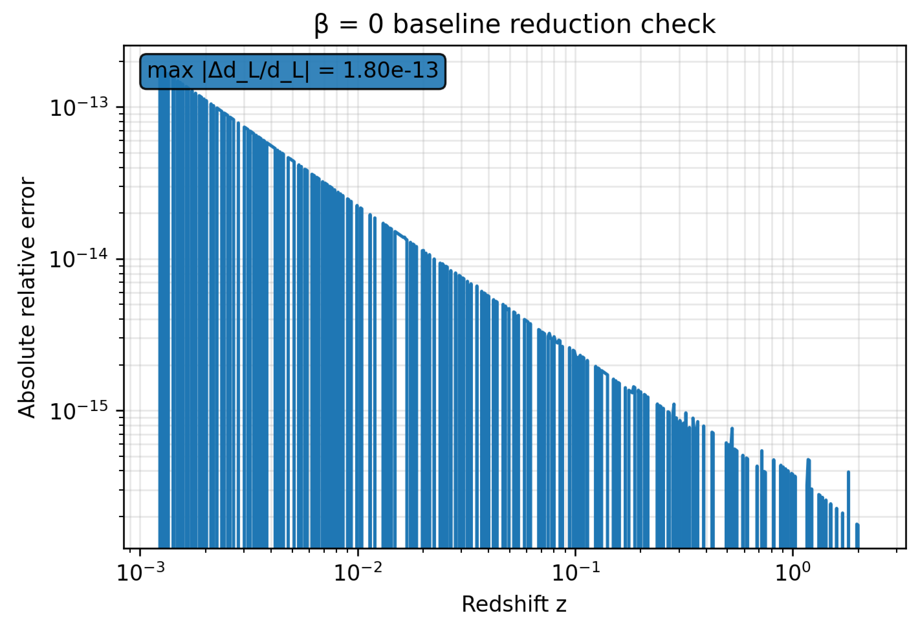
Figure 8.
Verification of continuity at (): absolute relative error between the form of Equation (7) evaluated at and the logarithmic limit . The redshift and error axes are logarithmic.
Figure 8.
Verification of continuity at (): absolute relative error between the form of Equation (7) evaluated at and the logarithmic limit . The redshift and error axes are logarithmic.
3.6. Implementation Verification Figures
4. Discussion
The Pantheon+SH0ES Hubble diagram admits a high-quality fit within a one-parameter unified-flow model in which a constant exponent modifies the distance–redshift relation through Equations (1)–(7). The model comparison metrics in Table 1 indicate strong preference for the variable- fit relative to the fixed-constants baseline under the AIC. Residual diagnostics show no pronounced redshift-dependent structure under a split at and give a whitened WRMS close to unity (Table 2), consistent with a statistically adequate covariance-weighted fit.
4.1. Interpretation of Information-Criterion Preference for Variable
The fixed-constants baseline at contains only the offset M and can therefore adjust the vertical normalization of the Hubble diagram but not its curvature with redshift. Allowing to vary changes the exponent in the light-propagation factor (Equation (4)), which directly controls the redshift dependence of the integrated distance scale in Equation (5). The large decrease in chi-squared relative to the baseline indicates that the Pantheon+SH0ES distance moduli require a redshift-dependent departure from the matter-only distance law beyond an intercept shift. Under the Akaike information criterion, the penalty for one additional parameter is 2, which is negligible compared with the observed improvement ; consequently, is dominated by the change in fit quality.
Empirically, the fitted value primarily captures the smooth, monotonic deviation of from the prediction at intermediate and high redshift, while the low-z normalization remains absorbed by the profiled offset M. Within the adopted ansatz, preference for is therefore a quantitative constraint on the redshift scaling required to reproduce the SN Ia Hubble diagram, rather than a standalone demonstration of variation in any particular dimensional constant.
4.2. Directionality and Example Scalings
Because , the flow factor satisfies for and therefore implies , , and toward the past (higher redshift), directly from Equation (2). For illustration at (so ), the best fit gives
The interpretation of changes in dimensional constants must ultimately be expressed in terms of dimensionless observables [20,21]. In this parameterization, the observational content is fully encoded by the modified luminosity-distance relation and the fitted exponent ; the scalings in Equation (2) should be read as an effective parameterization that reproduces the SN Hubble diagram within the assumed framework.
4.3. Scope Limitation: Constant for One Dataset
The parameter is treated as constant across the Pantheon+SH0ES sample, and the inference should be interpreted strictly within that modeling choice and dataset. The results establish that a constant- unified-flow parameterization fits this dataset and is strongly preferred to the fixed-constants baseline under AIC. No claim is made that a single exponent must describe all cosmological datasets or that cannot vary with redshift; testing , alternative functional forms for , or joint fits including other probes constitutes distinct empirical hypotheses.
4.4. Kinematic Interpretation from the Fitted Exponent
The fitted exponent fixes a simple kinematic interpretation for the background expansion implied by Equation (3). Writing gives , which corresponds to a constant deceleration parameter
At the best fit, , which is strictly decelerating () despite reproducing the observed SN Ia Hubble diagram. Formally, if the same power-law were re-expressed within a constant-w FLRW parameterization with fixed constants, implies an effective equation-of-state mapping
so that for the present fit. This mapping is an algebraic equivalence for only; a complete dynamical theory is required to interpret in terms of microphysics.
4.5. Sensitivity to the Covariance Structure
The main results use the full statistical+systematic covariance matrix supplied with Pantheon+SH0ES. As a robustness check, a diagonal-only fit was computed by replacing with while retaining the same distance model and analytic profiling of M. The diagonal-only best fit is with a 68% profile interval . The agreement between and indicates that the preferred exponent is not primarily driven by off-diagonal correlations, while the wider full-covariance uncertainty reflects the information loss associated with correlated systematics.
4.6. Standard-Model Benchmark and Discriminating Predictions
For context, a flat CDM benchmark was fitted to the same Pantheon+SH0ES distance moduli using the same full covariance matrix and the same analytic profiling of the offset M. The dimensionless luminosity distance proxy is
The integral in Equation (27) was evaluated by trapezoidal quadrature on a dense redshift grid and linearly interpolated to the observed redshifts; convergence was verified by grid refinement.
The best-fit flat CDM parameter is (68% profile interval), with for (Table 4). Because both unified flow and flat CDM employ one shape parameter plus the same offset M, their information criteria differ only by . The unified-flow fit improves the SN-only by relative to the flat CDM benchmark, indicating near-degeneracy at current SN precision.
Despite comparable fit quality, the two distance laws separate at the highest redshifts. After profiling M in both models, the predicted difference in distance modulus is , which reaches at the highest-redshift Pantheon+SH0ES object and grows to and under direct extrapolation (Figure 9). High-redshift standard candles or standard sirens can provide a direct discriminant between the two distance laws, because the predicted separation grows with redshift even when both models fit existing SN data well.
4.7. Relation to Other Constraints and External Observations
Laboratory and Solar-System tests, including lunar laser ranging and binary-pulsar timing, constrain departures from standard gravitational dynamics in the contemporary epoch [28,29,30]. Geophysical and spectroscopic measurements provide complementary limits on the variation of dimensionless parameters [31,32,33,34,35]. Early-Universe physics also constrains variations through nucleosynthesis and related processes [36,37]. Mapping the present phenomenological constraint to these bounds requires a complete dynamical theory specifying how dimensionless couplings evolve and how local time derivatives relate to redshift, which is not attempted here.
The unified-flow fit provides an observationally grounded alternative explanation of SN dimming without introducing an explicit dark-energy component. Contextual motivations for exploring such alternatives include empirical tensions and open questions in early structure formation. Several JWST analyses have reported candidate galaxies with high inferred stellar masses at [38,39], while subsequent studies have emphasized the role of selection effects, dust, and interloper contamination [40]. No quantitative analysis of these external datasets is performed; the SN result is presented as an internally consistent, covariance-respecting fit that motivates broader multi-probe tests.
5. Conclusions
A one-parameter unified-flow model with flow factor provides a statistically strong description of the Pantheon+SH0ES SN Ia Hubble diagram when the full covariance matrix is used. With SNe over , the best fit is under the modeling choice that is constant across this dataset. Residual diagnostics provide no indication of pronounced redshift-dependent structure under the adopted tests (Table 2). Within the adopted matter-closure kinematics, the fitted exponent corresponds to a constant deceleration parameter while reproducing the SN Ia Hubble diagram, indicating that the Pantheon+SH0ES distances can be fit without introducing an explicit dark-energy term within this phenomenological distance law. A supernova-only flat CDM benchmark fit yields a statistically indistinguishable goodness of fit (Table 4), but the two distance laws predict increasing separation at (Figure 9), enabling direct falsification with higher-redshift standard candles or standard sirens. Extending the test to additional probes and to more general forms remains a direct next step for empirical evaluation.
Author Contributions
Conceptualization, J.Y.; methodology, J.Y.; software, J.Y.; validation, J.Y.; formal analysis, J.Y.; investigation, J.Y.; writing—original draft preparation, J.Y.; writing—review and editing, J.Y.
Funding
This research received no external funding.
Institutional Review Board Statement
Not applicable.
Informed Consent Statement
Not applicable.
Data Availability Statement
Pantheon+ and Pantheon+SH0ES supernova data products and covariance matrices are publicly available with the Pantheon+ release [22]. The SH0ES distance-ladder analysis motivating the subset naming is described in [23]. Derived intermediate arrays and analysis scripts that reproduce the numerical results and figures are available from the corresponding author upon reasonable request.
Acknowledgments
This manuscript benefited from the use of artificial intelligence tools for grammatical refinement, improvements in clarity, and assistance with logical organization. All scientific content, interpretations, and conclusions are solely those of the author. The manuscript has undergone peer review and plagiarism screening by Editage.
Conflicts of Interest
The author declares no conflicts of interest.
References
- Hillebrandt, W.; Niemeyer, J. C. Type Ia supernova explosion models. Annu. Rev. Astron. Astrophys. 2000, 38, 191–230. [Google Scholar] [CrossRef]
- Maoz, D.; Mannucci, F.; Nelemans, G. Observational clues to the progenitors of Type Ia supernovae. Annu. Rev. Astron. Astrophys. 2014, 52, 107–170. [Google Scholar] [CrossRef]
- Phillips, M. M. The absolute magnitudes of Type IA supernovae. Astrophys. J. Lett. 1993, 413, L105–L108. [Google Scholar] [CrossRef]
- Tripp, R. A two-parameter luminosity correction for Type Ia supernovae. Astron. Astrophys. 1998, 331, 815–820. [Google Scholar]
- Guy, J.; Astier, P.; Baumont, S.; Hardin, D.; Pain, R.; Regnault, N.; Basa, S.; Carlberg, R. G.; Conley, A.; Fabbro, S.; et al. SALT2: Using distant supernovae to improve the use of Type Ia supernovae as distance indicators. Astron. Astrophys. 2007, 466, 11–21. [Google Scholar] [CrossRef]
- Hamuy, M.; Phillips, M. M.; Maza, J.; Suntzeff, N. B.; Schommer, R. A.; Aviles, R. A Hubble diagram of distant Type Ia supernovae. Astron. J. 1995, 109, 1–13. [Google Scholar] [CrossRef]
- Sullivan, M.; Ellis, R. S.; Nugent, P.; Smail, I.; Madau, P. The Hubble diagram of Type Ia supernovae as a function of host galaxy morphology. Mon. Not. R. Astron. Soc. 2003, 340, 1057–1075. [Google Scholar] [CrossRef]
- Krisciunas, K.; Phillips, M. M.; Suntzeff, N. B.; Persson, S. E.; Prieto, J. L.; Landolt, A. U. Hubble diagrams of Type Ia supernovae in the near-infrared. Astrophys. J. Lett. 2004, 602, L81–L84. [Google Scholar] [CrossRef]
- Stanishev, V.; Goobar, A.; Amanullah, R.; Bassett, B. A.; Fantaye, Y. T.; Garnavich, P. M.; Hlozek, R.; Nordin, J.; Okouma, P.; Östman, L.; et al. Type Ia supernova Hubble diagram with near-infrared and optical observations. Astron. Astrophys. 2018, 615, A45. [Google Scholar] [CrossRef]
- Riess, A. G.; Filippenko, A. V.; Challis, P.; Clocchiatti, A.; Diercks, A.; Garnavich, P. M.; Gilliland, R. L.; Hogan, C. J.; Jha, S.; Kirshner, R. P.; et al. Observational evidence from supernovae for an accelerating universe and a cosmological constant. Astron. J. 1998, 116, 1009–1038. [Google Scholar] [CrossRef]
- Perlmutter, S.; Aldering, G.; Goldhaber, G.; Knop, R. A.; Nugent, P.; Castro, P. G.; Deustua, S.; Fabbro, S.; Goobar, A.; Groom, D. E.; et al. Measurements of Ω and Λ from 42 high-redshift supernovae. Astrophys. J. 1999, 517, 565–586. [Google Scholar] [CrossRef]
- Weinberg, S. The cosmological constant problem. Rev. Mod. Phys. 1989, 61, 1–23. [Google Scholar] [CrossRef]
- Carroll, S. M. The cosmological constant. Living Rev. Relativ. 2001, 4, 1. [Google Scholar] [CrossRef] [PubMed]
- Joyce, A.; Lombriser, L.; Schmidt, F. Dark energy versus modified gravity. Annu. Rev. Nucl. Part. Sci. 2016, 66, 95–122. [Google Scholar] [CrossRef]
- Brans, C.; Dicke, R. H. Mach’s principle and a relativistic theory of gravitation. Phys. Rev. 1961, 124, 925–935. [Google Scholar] [CrossRef]
- Moffat, J. W. Superluminary universe: A possible solution to the initial value problem in cosmology. Int. J. Mod. Phys. D 1993, 2, 351–365. [Google Scholar] [CrossRef]
- Albrecht, A.; Magueijo, J. Time varying speed of light as a solution to cosmological puzzles. Phys. Rev. D 1999, 59, 043516. [Google Scholar] [CrossRef]
- Barrow, J. D. Cosmologies with varying light speed. Phys. Rev. D 1999, 59, 043515. [Google Scholar] [CrossRef]
- Magueijo, J. New varying speed of light theories. Rep. Prog. Phys. 2003, 66, 2025–2068. [Google Scholar] [CrossRef]
- Uzan, J.-P. Varying constants, gravitation and cosmology. Living Rev. Relativ. 2011, 14, 2. [Google Scholar] [CrossRef]
- Martins, C. J. A. P. The status of varying constants: A review of the physics, searches and implications. Rep. Prog. Phys. 2017, 80, 126902. [Google Scholar] [CrossRef] [PubMed]
- Scolnic, D.; Brout, D.; Carr, A.; Riess, A. G.; Davis, T. M.; Dwomoh, A.; Jones, D. O.; Ali, N.; Armstrong, P.; Carroll, R.; et al. The Pantheon+ analysis: The full data set and light-curve release. Astrophys. J. 2022, 938, 113. [Google Scholar] [CrossRef]
- Riess, A. G.; Yuan, W.; Macri, L. M.; Scolnic, D.; Brout, D.; Casertano, S.; Jones, D. O.; Murakami, Y.; Breuval, L.; Brink, T. G.; et al. A comprehensive measurement of the local value of the Hubble constant with 1kms-1Mpc-1 uncertainty from the Hubble Space Telescope and the SH0ES team. Astrophys. J. Lett. 2022, 934, L7. [Google Scholar] [CrossRef]
- Wilks, S. S. The large-sample distribution of the likelihood ratio for testing composite hypotheses. Ann. Math. Stat. 1938, 9, 60–62. [Google Scholar] [CrossRef]
- Akaike, H. A new look at the statistical model identification. IEEE Trans. Autom. Control 1974, 19(6), 716–723. [Google Scholar] [CrossRef]
- Burnham, K. P.; Anderson, D. R. Model Selection and Multimodel Inference: A Practical Information-Theoretic Approach, 2nd ed.; Springer: New York, NY, USA, 2002. [Google Scholar]
- Berger, V. W.; Zhou, Y. Kolmogorov–Smirnov Test: Overview. In Wiley StatsRef: Statistics Reference Online; Wiley: Hoboken, NJ, USA, 2014. [Google Scholar] [CrossRef]
- Will, C. M. The confrontation between general relativity and experiment. Living Rev. Relativ. 2014, 17, 4. [Google Scholar] [CrossRef]
- Hofmann, F.; Müller, J. Relativistic tests with lunar laser ranging. Class. Quantum Grav. 2018, 35, 035015. [Google Scholar] [CrossRef]
- Williams, J. G.; Turyshev, S. G.; Boggs, D. H. Progress in lunar laser ranging tests of relativistic gravity. Phys. Rev. Lett. 2004, 93, 261101. [Google Scholar] [CrossRef]
- Damour, T.; Dyson, F. The Oklo bound on the time variation of the fine-structure constant revisited. Nucl. Phys. B 1996, 480, 37–54. [Google Scholar] [CrossRef]
- Rosenband, T.; Hume, D. B.; Schmidt, P. O.; Chou, C. W.; Brusch, A.; Lorini, L.; Oskay, W. H.; Drullinger, R. E.; Fortier, T. M.; Stalnaker, J. E.; et al. Frequency ratio of Al+ and Hg+ single-ion optical clocks; constraints on the time variation of fundamental constants. Science 2008, 319, 1808–1812. [Google Scholar] [CrossRef]
- Godun, R. M.; Nisbet-Jones, P. B. R.; Jones, J. M.; King, S. A.; Johnson, L. A. M.; Margolis, H. S.; Szymaniec, K.; Lea, S. N.; Bongs, K.; Gill, P. Frequency ratio of two optical clock transitions in 171Yb+ and constraints on the time variation of fundamental constants. Phys. Rev. Lett. 2014, 113, 210801. [Google Scholar] [CrossRef]
- Murphy, M. T.; Webb, J. K.; Flambaum, V. V. Further evidence for a variable fine-structure constant from Keck/HIRES QSO absorption spectra. Mon. Not. R. Astron. Soc. 2003, 345, 609–638. [Google Scholar] [CrossRef]
- Webb, J. K.; King, J. A.; Murphy, M. T.; Flambaum, V. V.; Carswell, R. F.; Bainbridge, M. B. Indications of a spatial variation of the fine structure constant. Phys. Rev. Lett. 2011, 107, 191101. [Google Scholar] [CrossRef]
- Cyburt, R. H.; Fields, B. D.; Olive, K. A.; Yeh, T.-H. Big bang nucleosynthesis: Present status. Rev. Mod. Phys. 2016, 88, 015004. [Google Scholar] [CrossRef]
- Pitrou, C.; Coc, A.; Uzan, J.-P.; Vangioni, E. Precision big bang nucleosynthesis with improved helium-4 predictions. Phys. Rep. 2018, 754, 1–66. [Google Scholar] [CrossRef]
- Labbé, I.; van Dokkum, P.; Nelson, E.; Bezanson, R.; Brammer, G.; Whitaker, K. E.; Illingworth, G.; Muzzin, A.; Marchesini, D.; Franx, M.; et al. A population of red candidate massive galaxies ∼600 Myr after the Big Bang. Nature 2023, 616, 266–269. [Google Scholar] [CrossRef] [PubMed]
- Boylan-Kolchin, M. Stress testing ΛCDM with high-redshift galaxy candidates. Nat. Astron. 2023, 7, 731–735. [Google Scholar] [CrossRef]
- Zavala, J. A.; Aretxaga, I.; Hughes, D. H.; Béjar, V. J.; Bertoldi, F.; Chapin, E. L.; Dunlop, J. S.; Ivison, R. J.; Kneib, J.-P.; Michałowski, M. J.; et al. Dusty starbursts masquerading as ultra-high-redshift galaxies in JWST CEERS observations. Astrophys. J. Lett. 2023, 943, L9. [Google Scholar] [CrossRef]
Figure 1.
Pantheon+SH0ES distance moduli versus redshift with the unified-flow best-fit curve at . The redshift axis is logarithmic.
Figure 1.
Pantheon+SH0ES distance moduli versus redshift with the unified-flow best-fit curve at . The redshift axis is logarithmic.
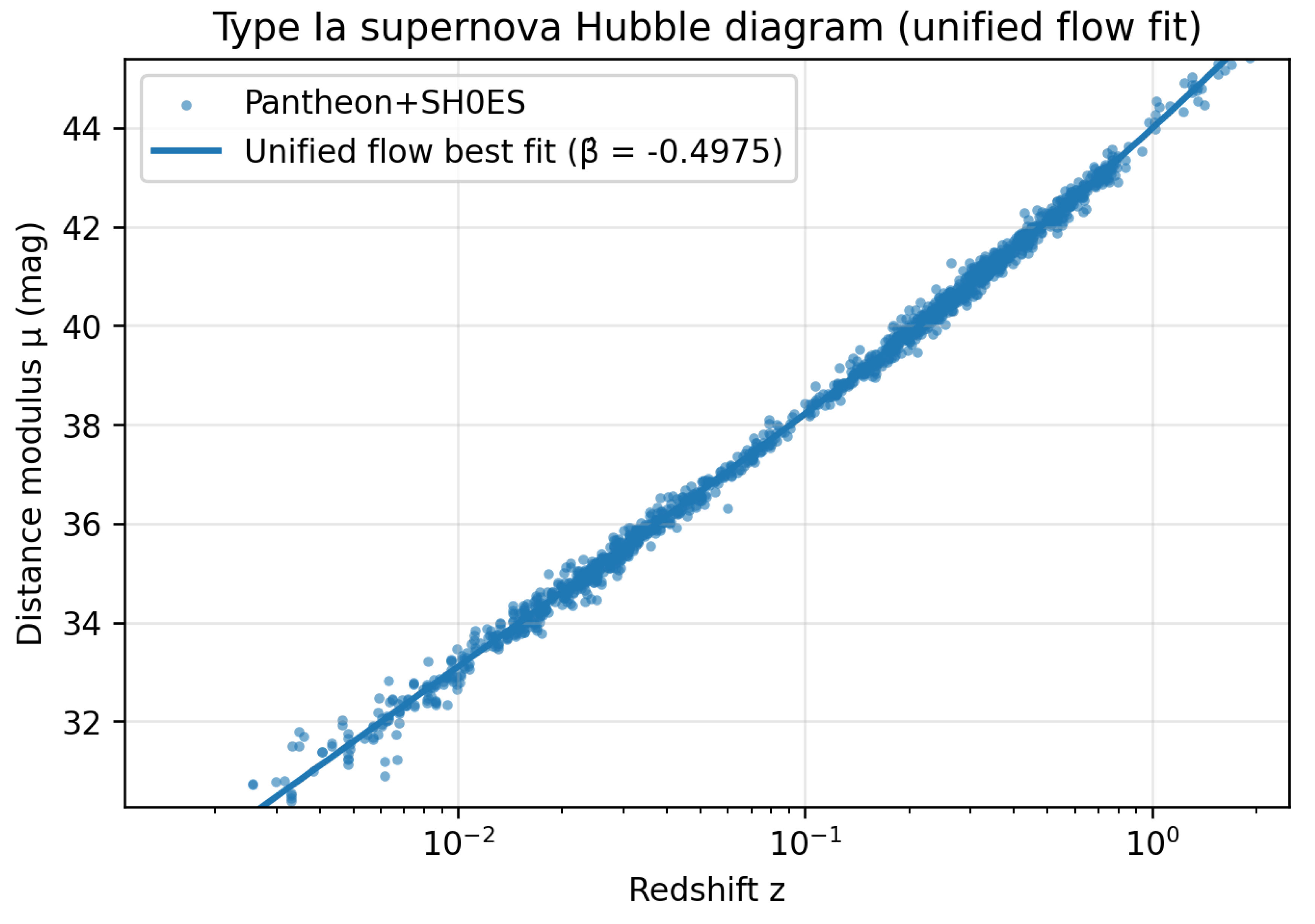
Figure 9.
Difference in distance modulus between the best-fit unified-flow model and the best-fit flat CDM benchmark, , after profiling the offset M in both models. The dashed vertical line marks the maximum redshift in Pantheon+SH0ES; the curve beyond this line is an extrapolation that provides a discriminating prediction for higher-redshift standard candles or standard sirens.
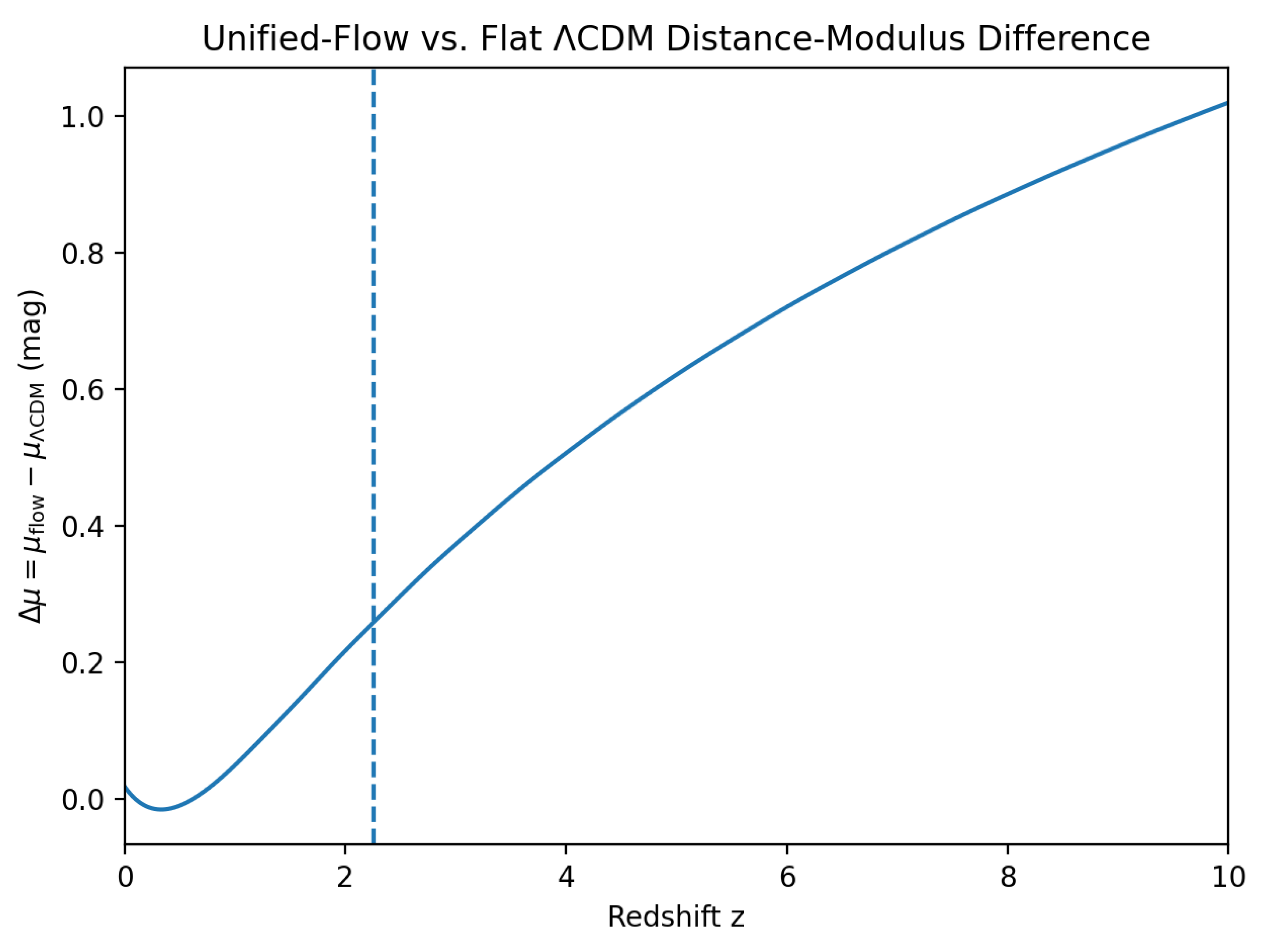

Table 1.
Fit summary for the unified-flow model (variable ) and the fixed-constants baseline (). The nuisance offset M is analytically profiled in both cases; denotes degrees of freedom and k the number of fitted parameters.
Table 1.
Fit summary for the unified-flow model (variable ) and the fixed-constants baseline (). The nuisance offset M is analytically profiled in both cases; denotes degrees of freedom and k the number of fitted parameters.
| Model | ||||||
|---|---|---|---|---|---|---|
| Unified flow | 1699 | |||||
| Fixed constants () | 0 | 1700 |
Table 2.
Residual diagnostics for the best-fit unified-flow model.
| Diagnostic | Value |
|---|---|
| Redshift split for KS test | |
| () | 1491 |
| () | 210 |
| KS statistic | |
| KS p-value | |
| WRMS |
Table 3.
Profile-likelihood confidence intervals for the unified-flow exponent (one-parameter thresholds).
Table 3.
Profile-likelihood confidence intervals for the unified-flow exponent (one-parameter thresholds).
| Level | threshold | Interval for |
|---|---|---|
| 68% | ||
| 95% |
Table 4.
Supernova-only benchmark comparison between the unified-flow distance law and a flat CDM distance law, using the full Pantheon+SH0ES statistical+systematic covariance matrix. Both models fit two parameters (shape parameter or and offset M).
Table 4.
Supernova-only benchmark comparison between the unified-flow distance law and a flat CDM distance law, using the full Pantheon+SH0ES statistical+systematic covariance matrix. Both models fit two parameters (shape parameter or and offset M).
| Model | Shape parameter | AIC | BIC | ||||
|---|---|---|---|---|---|---|---|
| Unified flow | 1699 | ||||||
| Flat CDM | 1699 |
Disclaimer/Publisher’s Note: The statements, opinions and data contained in all publications are solely those of the individual author(s) and contributor(s) and not of MDPI and/or the editor(s). MDPI and/or the editor(s) disclaim responsibility for any injury to people or property resulting from any ideas, methods, instructions or products referred to in the content. |
© 2026 by the authors. Licensee MDPI, Basel, Switzerland. This article is an open access article distributed under the terms and conditions of the Creative Commons Attribution (CC BY) license (http://creativecommons.org/licenses/by/4.0/).
Copyright: This open access article is published under a Creative Commons CC BY 4.0 license, which permit the free download, distribution, and reuse, provided that the author and preprint are cited in any reuse.


