Submitted:
08 February 2026
Posted:
10 February 2026
You are already at the latest version
Abstract
We present D2BIA_discrete, a zero-cost computational framework for predicting local aromaticity in linear acenes without quantum chemical calculations. The model partitions π-electron density using a 61/39 localized/delocalized ratio derived from spin-coupled valence bond and QTAIM analyses, combined with Slater-type orbital decay to estimate ring-center electron density. Three progressive refinements introduce molecular topology weighting, tunable bond-sharing (α), and depth-dependent attenuation (γ) parameters. Leave-one-n-out cross-validation on benzene through undecacene yields optimal parameters α=1.00 and γ=0.05, achieving ring-by-ring predictions with R²=0.456 and RMSE=2.394×10⁻³ against fluorescence aromaticity index (FLU). Model 2 provides excellent molecular-averaged correlations (R²>0.93 for FLU, PDI, HOMA) and reliable ring-level predictions for terminal and first internal rings. Local LONOCV D2BIA_discrete has excellent metrics with six-center index (R² = 0.922, R = 0.960, RMSE = 0.219, MAE = 0.139, MRE = 4.83%), showing importance of zero-cost D2BIA_discrete to obtain local aromaticity of linear acenes in agreement with SCI gradients for the same group. This is our third work based on the so-called discrete geometry chemistry.
Keywords:
D2BIA
; six-center index
; aromaticity index
; linear acenes
; discrete geometry chemistry
Introduction
Linear acenes—polycyclic aromatic hydrocarbons composed of linearly fused benzene rings—have garnered significant attention due to their unique electronic properties and potential applications in organic electronics. Pentacene and its derivatives serve as benchmark materials in organic field-effect transistors (OFETs), exhibiting charge carrier mobilities comparable to amorphous silicon. [1,2]As chain length increases from benzene to larger acenes, systematic changes occur in their band gaps, charge transport properties, and photophysical characteristics, making them ideal model systems for studying π-conjugation and aromaticity.[3] Beyond their application in OFETs, acenes have shown promise in organic photovoltaics[4] (OPVs), sensors,[5] and stimuli-responsive materials.[2] Polycyclic aromatic hydrocarbons (PAHs) constitute a broader class of conjugated molecules with diverse structural topologies—linear, angular, and complex fused arrangements—whose applications extend to energy storage,[6] nanographene-based materials,[7] sensors for volatile organic compounds,[5] and advanced optoelectronic devices.[7] The tunable electronic properties of PAHs through molecular engineering make them versatile platforms for developing next-generation materials with applications ranging from molecular electronics to biological sensing.
Aromaticity, a fundamental concept describing the enhanced stability and unique reactivity of cyclic π-conjugated systems, plays a crucial role in understanding and predicting the properties of PAHs and related materials. Since Hückel's formulation of the 4n+2 rule,[8] numerous quantitative indices have been developed to characterize aromaticity based on different physical manifestations. The fluctuation index (FLU) measures the variance of electron delocalization indices between adjacent atoms relative to benzene as reference, with lower values indicating higher aromaticity.[9] The para-delocalization index (PDI) evaluates electron sharing between para-related carbon atoms in six-membered rings, providing insight into through-ring π-electron delocalization.[10] The six-center index (SCI), based on generalized population analysis or multicenter delocalization measures, quantifies the degree of electron delocalization across all six atoms of a benzene ring.[11,12] Geometric criteria include the harmonic oscillator model of aromaticity (HOMA), which quantifies bond length equalization by comparing carbon-carbon distances to optimal aromatic values, with HOMA = 1 for perfect benzene-like aromaticity and HOMA = 0 for hypothetical cyclohexatriene.[13] Magnetic criteria are represented by nucleus-independent chemical shift (NICS) values, calculated as the negative of the absolute magnetic shielding at ring centers or specific positions above the ring plane, with more negative values indicating greater diatropic ring current and aromaticity. [14,15] Beyond these established indices, topological approaches have emerged. D3BIA (density, degeneracy, and delocalization-based index of aromaticity) combines electron density at ring critical points, orbital degeneracy, and QTAIM delocalization indices to provide a reference-independent measure of aromaticity applicable to diverse aromatic systems.[16,17] Its improved version, D2BIA,[18] eliminates the arbitrary degeneracy term while maintaining effectiveness across planar and non-planar aromatic systems, showing excellent correlations with FLU and NICS for benzenoid rings, heteroaromatics, and homoaromatic compounds. While these indices approach aromaticity from different perspectives—electronic, geometric, magnetic, or topological—their complementary use provides comprehensive characterization of aromatic character in complex molecular systems.
Discrete-geometry chemistry represents an emerging computational paradigm that simplifies complex quantum mechanical models by employing discrete geometric representations and discrete numerical parameters to transform computationally expensive problems into tractable ones. This approach is grounded in mathematical principles of discrete mathematics and graph theory, where molecular topology is encoded through discrete numbers—such as connectivity indices, vertex positions, or quantized physical parameters—rather than continuous functions requiring full quantum mechanical treatment. The fundamental strategy involves constructing simplified models based on fixed electronic positions and discrete geometric configurations, then validating these models through train-test-validation protocols against experimental or high-level computational benchmarks. The Snapshot Coulombic model for linear conjugated oligoenes exemplifies this paradigm.[19] In this 1D model, π-electrons are positioned at fixed distances (re = 0.60 Å) from carbon nuclei arranged linearly along the conjugated chain, with each carbon assigned an effective nuclear charge (Zeff = 3.25) derived from Slater's rules. The total electrostatic potential energy V(r), calculated as the sum of attractive electron-nucleus and repulsive nucleus-nucleus interactions, exhibits logarithmic correlations with experimental maximum UV absorption wavelengths (λmax) of oligoenes (R² = 0.98) and with heat of combustion of oligoynes, despite the model's extreme simplification. The 2D Snapshot Coulombic extension adapts this framework for PAHs by incorporating topological factors reflecting the two-dimensional arrangement of fused aromatic rings. By weighting the electron-nucleus interactions according to structural topology—accounting for ring fusion patterns, symmetry, and connectivity—the 2D model's V(r) values demonstrate strong correlations with ionization energy and fundamental gap energy of PAHs.[20] Both models share the discrete-geometry philosophy: fixed electron positions, discrete geometric parameters (nuclear charges, distances), and empirical validation bridging simplified discrete representations to complex quantum reality. This approach offers computational efficiency while maintaining predictive accuracy for specific molecular properties.
This work introduces D2BIA_discrete, a zero-cost computational model for predicting local aromaticity in linear acenes without quantum chemical calculations. Building upon discrete-geometry chemistry principles, D2BIA_discrete employs fixed discrete geometric parameters—π-electron positions derived from QTAIM ring critical point densities, discrete bond-sharing ratios based on spin-coupled valence bond theory (61% localized / 39% delocalized), and topological connectivity numbers (number of fused bonds per ring)—to estimate ring-center electron density. Similar to the Snapshot Coulombic models, the discrete representation (Figure 1 of manuscript) uses fixed electron-nucleus distances and simplified electrostatic descriptions, validated through train-test protocols on acene series from benzene to undecacene. Three progressive model refinements introduce: (1) basic ring-center density calculation; (2) molecular topology weighting via w(n) factor; and (3) tunable bond-sharing (α) and depth-attenuation (γ) parameters optimized through leave-one-n-out cross-validation. The model achieves ring-by-ring aromaticity predictions correlating with established indices (FLU, PDI, HOMA, NICS(1)zz) while requiring only molecular connectivity information, demonstrating the viability of discrete-geometry approaches for rapid aromaticity assessment in extended π-systems.
Rationale For D2BIA_Discrete Models
2.1. D2BIA_dicrete: Model 1
The development of the D2BIA_discrete index begins with the recognition that existing aromaticity indices based on quantum topological analyses, while chemically insightful, require computationally expensive electron density calculations. The original D3BIA index[21,22], validated for benzenoid systems in 2015, combines three factors through the product
where RDF represents the ring density factor computed as RDF = (1 + λ₂)ρRCP for planar aromatics, DIU measures delocalization index uniformity defined as DIU = 100 − 100(σ/DIavg) with σ denoting the mean deviation and DIavg the average of delocalization indices for bonded atom pairs in the ring circuit, and δ represents the degeneracy factor computed as δ = n/N based on empirical rules for identifying degenerate or quasi-degenerate atoms. In this formulation, ρRCP is the electron density at the ring critical point, λ₂ is the average of the second eigenvalue of the density Hessian at bond critical points with eigenvector pointing toward the ring center, and for linear acenes δ equals unity since all carbon atoms in the ring are treated as equivalent.
D3BIA = RDF · DIU · δ,
The 2017 refinement[18] introduced D2BIA by eliminating the degeneracy term δ, which was considered arbitrary and difficult for new users to apply consistently, yielding the simplified two-component product
D2BIA(p) = [(1 + λ₂)ρ_RCP] · DIU ,
Both formulations, however, still require extraction of delocalization indices from Quantum Theory of Atoms in Molecules analyses and critical point properties from the electron density topology, motivating the search for a discrete surrogate that preserves the conceptual structure while eliminating these computational dependencies.
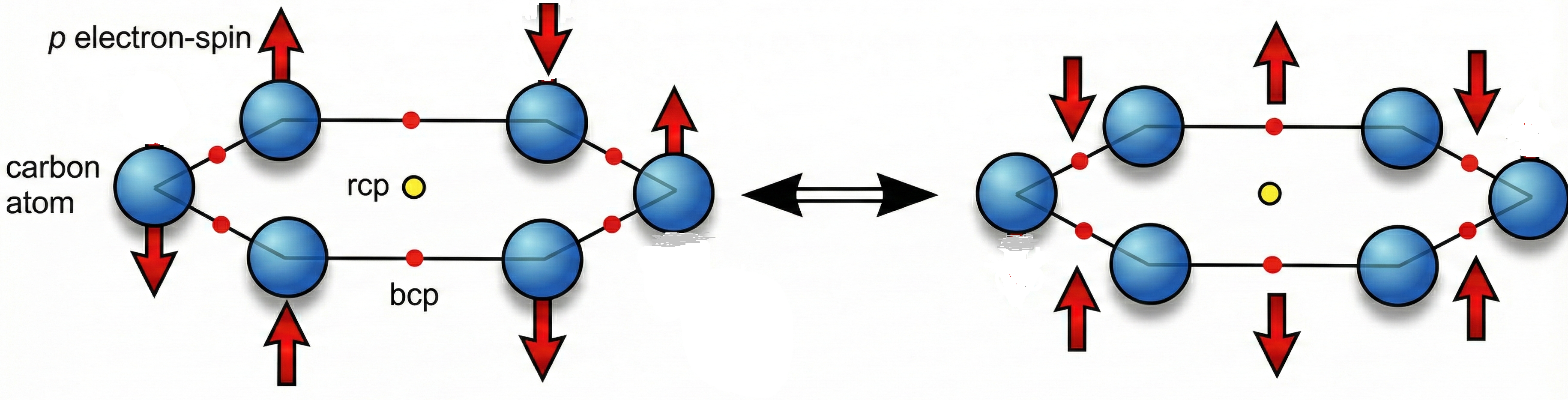
The discrete model construction proceeds by identifying the two fundamental physical components that D2BIA captures: the concentration of π electron density at the ring center, which we denote as the internal density factor or IDF, and the uniformity of π electron distribution around the ring perimeter, quantified through DIU. To construct discrete approximations for these quantities without resorting to wavefunction-based calculations, we turn to theoretical analyses that provide interpretable partitioning of electron localization. Spin-coupled valence bond calculations for benzene[23] reveal that the π system is well described by singly occupied p orbitals localized primarily on individual carbon atoms with modest delocalization tails extending to neighboring carbons. This picture finds quantitative support in Quantum Theory of Atoms in Molecules partitioning, which assigns a delocalization index DI(C−C) ≈ 1.39e for each carbon-carbon bond in benzene, where e is the eletron charge. When the σ bond contribution of 1.0e is subtracted, the residual π contribution is approximately 0.39 electrons shared between the two carbons forming the bond. The complement, 1.00 − 0.39 = 0.61e, then represents the π electron density localized on each carbon atom.[21] This 61/39 partitioning between atomic localization and bond delocalization provides the empirical foundation for our discrete electron distribution model. The convergence of two independent theoretical approaches, one based on variational wavefunction construction (spin-coupled VB) and the other on rigorous density partitioning (QTAIM), lends confidence that this partitioning captures genuine physical content rather than method-dependent artifacts. Figure 1 depitcs the conceptual distribution of Csp2 π-electrons along the benzene ring with pictorial representation of ring critical point, rcp, and bond critical points, bcp, from QTAIM perspective. It has two resonant structures with distinguished weights/coefficients: 0.61 and 0.39.
Based on this 61/39 partitioning, we construct a discrete representation of π electron distribution for benzene (Figure 1). For a (benzene or a more generically benzenoid) ring with six carbon atoms labeled C₁ to C₆ in a cyclic sequence, the discrete contribution of the i-th π electron is written as
where Ci denotes the position vector of the i-th carbon atom, C{i+1} denotes the position of the next carbon in the cycle with the periodic boundary condition C₇ ≡ C₁, and the notation (Ci − C{i+1}) represents the bond region between consecutive carbons rather than a vector subtraction. The coefficient 0.61 weights the contribution localized at the carbon center, while 0.39 weights the contribution in the C−C bond region.
eπ(i) = 0.61Ci + 0.39(Ci − C{i+1}),
For the complete benzene system containing six π electrons, the total π distribution is obtained by summing over all six electron positions to yield:
This expression provides a discrete accounting of how the six π electrons are partitioned between atomic centers and bond regions, serving as the starting point for estimating the discrete π density at the ring center.
To convert this discrete electron distribution into a quantitative estimate of ring-center density, we adopt an exponential decay model inspired by Slater-type orbital behavior.[24] The amplitude of π electron density at distance r from a carbon atom is assumed to decay exponentially as exp(−ζr), where ζ is the orbital decay exponent characterizing the spatial extent of carbon 2p orbitals. For carbon π orbitals, theoretical estimates suggest ζ ≈ 3.07 Å⁻¹ as a representative value. Taking r₀ = 1.20 Å as the approximate distance from a carbon atom to the geometric center of a benzene ring, the amplitude reaching the center from a single electron localized at one carbon is computed as exp(−3.07 × 1.20) = exp(−3.684) ≈ 0.02509. This numerical value becomes the fundamental amplitude constant k = 0.02509 in our discrete model.
For benzene, where the ring has perfect hexagonal symmetry, each of the six carbon atoms contributes 0.61 of a localized π electron, and each of the six C−C bonds contributes 0.39 of a shared π electron. The total effective π amplitude sum reaching the ring center, denoted S, equals 6 for the symmetric benzene case. The electron density at the ring center is then approximated as
where the square reflects the fact that electron density is proportional to the square of the wavefunction amplitude. For benzene, this yields ρcenter = (0.02509 × 6)² = (0.15054)² ≈ 0.02266, providing the initial estimate of ring-center density from purely discrete counting.
ρcenter = (kS)²,
S =6, for benzene, ρcenter(benzene)= (6× 0.02509)2 = 0.02266
The delocalization index uniformity, DIU, quantifies how evenly π electrons are distributed around the ring perimeter. In the original D2BIA formulation, DIU is computed from the variance of delocalization indices for adjacent atom pairs in the ring. In our discrete model, we approximate DIU by counting the effective number of bonds contributing to the ring. For an isolated benzene ring where all six C−C bonds are equivalent and fully internal to the ring, the effective bond sum is S = 6, and we define
representing maximal uniformity.
DIU(benzene) = S/6 = 1.0, where S=6,
When rings are fused to neighboring rings in polycyclic systems, certain bonds become shared between two rings, reducing their effective contribution to each individual ring, and as a consequence, reducing the DIU of each fused ring. The simplest approximation assigns each fused bond a weight of 0.5 to each of the two rings it connects. For a ring with f fused bonds and (6−f) non-fused bonds, the effective bond sum becomes
and the uniformity factor is
S = (6−f) + f × 0.5 = 6 − 0.5f,
DIU = S/6 = 1 − f/12,
This construction ensures that terminal rings in acenes, which have f = 1 fused bond, receive DIU = 5.5/6 ≈ 0.917, while internal rings with f = 2 fused bonds receive DIU = 5.0/6 ≈ 0.833, capturing the intuitive notion that rings with more fused bonds have less uniform π distribution due to bond-sharing competition with neighbors.
Combining these components, the initial discrete aromaticity index for a ring is constructed as the product
D2BIA_discrete = DIU × ρcenter= (S/6) × (kS)²,
This formulation mirrors the structure of the original D2BIA index as the product of a uniformity measure and a density factor, but replaces quantum topological observables with purely combinatorial quantities derived from molecular graph structure. For benzene as the reference case, we obtain D2BIA_discrete = 1.0 × (0.02509 × 6)² ≈ 0.02266. For naphthalene, each of the two equivalent rings has f = 1 fused bond, giving S = 5.5, DIU = 0.917, ρcenter = (0.02509 × 5.5)² ≈ 0.01904, and D2BIA_discrete ≈ 0.01746. For the terminal rings of anthracene, the same calculation yields D2BIA_discrete ≈ 0.01746, while the central ring with f = 2 gives S = 5.0, DIU = 0.833, ρcenter ≈ 0.01574, and D2BIA_discrete ≈ 0.01311. This initial version successfully differentiates terminal from internal rings based solely on fused bond counting, providing a first discrete approximation to local aromaticity variation in acene chains.
Table 1 presents the calculated D2BIA_discrete values for the first four linear acenes, demonstrating how the index captures the distinction between terminal and internal ring positions. For benzene, the single ring yields D2BIA = 0.02266 with maximal uniformity DIU = 1.0000 and effective amplitude sum e(∑,1.20) = 0.15054. In naphthalene, both rings are equivalent with one fused bond each, producing DIU = 0.9167 and D2BIA = 0.01746 per ring. Anthracene exhibits the first differentiation between ring types: the two terminal rings retain the same values as naphthalene rings (D2BIA = 0.01746), while the central ring with two fused bonds shows reduced uniformity DIU = 0.8333, lower effective amplitude e(∑,1.20) = 0.12545, and consequently reduced D2BIA = 0.01311. This pattern continues in tetracene, where the two terminal rings maintain D2BIA = 0.01746 while the two internal rings each exhibit the reduced value D2BIA = 0.01311. The systematic decrease in D2BIA from terminal to internal positions reflects the physical expectation that rings with more fused bonds experience greater competition for π electron density and reduced aromaticity, establishing the discrete index as a computationally trivial yet chemically meaningful probe of local aromatic character in linearly fused benzenoid systems.
2.2. D2BIA_Dicrete: Model 2 – Refinement with Weighted Values
A critical refinement recognizes that as acene chains grow longer, the total number of π electrons Nπ = 4n + 2 increases linearly with the number of rings n, while the number of rings also increases, causing the average number of π electrons per ring to decrease according to Nπ/n = (4n + 2)/n. For benzene with n = 1, this ratio is 6 electrons per ring, but for naphthalene with n = 2 it drops to 5 electrons per ring, for anthracene with n = 3 it is 14/3 ≈ 4.67 electrons per ring, and as n grows large the ratio asymptotically approaches 4. To account for this global topological effect, we introduce a molecular weighting factor
which equals 1.0 for benzene, 5/6 ≈ 0.833 for naphthalene, 7/9 ≈ 0.778 for anthracene, and 3/4 = 0.750 for tetracene. This weight factor is applied uniformly to all rings in a given n-acene, scaling the discrete index to
w(n) = [(4n + 2)/n]/6 = (4n + 2)/(6n),
D2BIA_discrete = w(n) × DIU × ρcenter. ,
This modification represents the first major improvement to the discrete formulation, ensuring that the index properly reflects the decreasing per-ring π electron availability as molecular size increases. With this global weight incorporated, the complete initial discrete index is defined as
where w(n) = (4n + 2)/(6n), S = 6 − 0.5f for a ring with f fused bonds, k = 0.02509 is the amplitude constant, and all quantities are determined purely from molecular topology without requiring any quantum chemical calculations.
D2BIA_discrete = w(n) × (S/6) × (kS)²,
Table 2 demonstrates the effect of incorporating the topological weight w(n) into the D2BIA_discrete calculation for acenes from benzene to pentacene. The unweighted D2BIA values (before applying w(n)) depend only on the ring's local fused-bond count f, resulting in just two distinct values across all acenes: 0.01746 for terminal rings (f = 1) and 0.01311 for internal rings (f = 2), with benzene as a special case at 0.02266 (f = 0). Application of the weight factor w(n) scales these values downward as chain length increases, properly accounting for the dilution of π electron density across growing numbers of rings. For naphthalene with w(2) = 0.833, the terminal ring values reduce from 0.01746 to 0.01455. In anthracene with w(3) = 0.778, terminal rings scale to 0.01358 while the central ring drops to 0.01020. This trend continues through tetracene (w(4) = 0.750) and pentacene (w(5) = 0.733), where terminal rings reach 0.01280 and internal/central rings fall to 0.00962. The weighted formulation ensures that longer acenes, despite having identical local ring topologies to shorter homologues, correctly exhibit reduced per-ring aromaticity indices reflecting their lower π electron density per ring, making D2BIA_discrete values properly comparable across the entire acene series and enabling meaningful correlations with experimental aromaticity measures that span multiple chain lengths.
We tested the refined D2BIA_discrete model (model 2) incorporating the topological weight w(n) against four established aromaticity indices for linear acenes. As to local analysis (ring-by-ring) Model 2 yields poor correlation coefficients R² = 0.316 for HOMA, R² = 0.225 for NICS(1) and only a good relation with PDI (R² = 0.861). The PDI x Model 2 relation demonstrates that the discrete model successfully captures delocalization-based aromaticity measures, while the weaker correlations with HOMA and NICS(1) indicate that these indices respond to additional geometric and magnetic shielding effects not fully represented by the simple fused-bond counting and exponential decay framework. These initial ring-by-ring validation results established that further refinement was necessary to improve the model's generality across multiple aromaticity criteria, motivating the development of Model 3 with variable bond-sharing and depth-penalty parameters.
2.3. D2BIA_Discrete: Model 3 – Introduction of Tunable Parameters α and γ
The initial models successfully captured the qualitative distinction between terminal and internal rings through fixed bond-sharing rules and global π electron weighting, but two fundamental limitations remained. First, the assumption that each fused bond contributes exactly 0.5 to each adjacent ring, while mathematically convenient, lacks empirical justification and may not represent the true partitioning of π electron density in polycyclic systems. Second, the models treated rings at different positions along the acene backbone identically if they shared the same number of fused bonds, failing to account for the intuitive expectation that rings deeper within the molecular interior should exhibit reduced ring-center π density due to increased structural constraint and electronic competition. These limitations motivated the development of Model 3, which introduces two physically interpretable, tunable parameters α and γ that generalize the bond-sharing and depth-dependent effects while maintaining the discrete mathematical framework.
The parameter α, termed the bond-sharing parameter, replaces the fixed 0.5 weighting with a variable coefficient controlling the effective contribution of fused bonds to ring π electron count. The effective bond sum S for a ring with f fused bonds is:
where α ∈ [0,1] represents the fraction of each fused bond that "belongs" to the ring for purposes of electron counting. The value of this parameter is obtained through grid optimization based on coefficients of determination of D2BIA_discrete with well-known aromaticity indices.
S = (6 − f) + fα,
The uniformity factor DIU remains DIU = S/6, but now depends on α through S. When α = 0.5, the model reduces to the fixed bond-sharing case of model 2, providing continuity with previous formulations. When α approaches 1, each fused bond is treated almost as if fully assigned to each ring, representing maximal local electron availability despite the shared bond. When α approaches 0, fused bonds contribute minimally to the ring electron count, representing strong delocalization away from individual rings into the fused bond region. The physical interpretation of α is that it quantifies the extent to which π electrons in fused bonds remain localized within individual ring environments (α = 1) versus being shared diffusely across multiple rings (0 ≤ α < 1), with the optimal value determined empirically from training data rather than imposed a priori.
The parameter γ, termed the depth-decay parameter, introduces position-dependent modulation of ring-center electron density based on the discrete distance of each ring from the molecular periphery. For a linear n-acene with rings indexed p = 1, ..., n, we define the depth index, d(p), as
which measures the minimum number of ring steps from ring p to either chain terminus. Terminal rings have d = 0, the first internal rings have d = 1, and the central ring in an odd-acene chain has d = max, equal to floor(n/2). The depth index, is the minimum number between p-1 and n-p. For example, if n = 3 and p = 1 (e.g., in the first terminal ring of anthracene), p-1 = 0 and n-p = 2, then d = 0. For the cenral ring of anthracene, n=3 and p=2, p-1 =1 and n-p = 1, then d = 1.
d(p) = min(p − 1, n − p),
The depth factor, g(p), is defined as
where γ ≥ 0 is the decay rate parameter. This exponential form ensures that g = 1 for terminal rings (no penalty), decays smoothly as rings move inward, and approaches zero for deeply buried rings if γ is large. The ring-center density is then modified to
incorporating both the amplitude-based density (kS)² and the depth-dependent attenuation g(p).The purpose of the g(p) attenuation is to account for the decrease in π electron density at the ring center as the ring position becomes more internal within the acene chain, reflecting increased structural constraint and electronic competition in deeply buried rings.
g(p) = exp(−γd(p)),
ρcenter = g(p) · (kS)²,
The complete D2BIA_discrete expression for Model 3 becomes
where all components now depend explicitly on the tunable parameters through S(α) and g(d(p); γ).
D2BIA_discrete(n,p; α,γ) = w(n) · (S/6) · [g(p) · (kS)²],
The calibration of α and γ requires a systematic search over parameter space guided by quantitative comparison with established aromaticity indices. The training data consist of ring-averaged (and not local ring) aromaticity descriptors PDI, FLU, HOMA, and NICS(1)_zz for linear acenes with n = 1 to n = 10 rings obtained from Donghai and coworkers.[25] For each acene of size n, the ring-averaged values are computed by averaging over all rings in the molecule, accounting for the symmetric equivalence of terminal and internal positions. The parameter optimization employs a brute-force two-dimensional grid search algorithm that exhaustively evaluates model performance across a dense parameter grid in (α, γ) space, selecting the combination (α*, γ*) that maximizes a composite score reflecting agreement with multiple aromaticity criteria simultaneously. The objective function is defined as a weighted sum of determination coefficients:
where m ∈ {PDI, FLU, HOMA, NICS} and λm ≥ 0 are user-defined weights reflecting the relative importance of each aromaticity descriptor. For balanced multi-index optimization, equal weights λm = 1 are employed. Alternatively, the objective function can be formulated to minimize RMSE after linear rescaling if the indices differ greatly in magnitude.
Grid Search Optimization of Parameters α and γ
The grid search algorithm operates as follows. First, it constructs the α-grid as a uniformly spaced array of 191 points spanning the interval [0, 1], yielding α-values at increments of approximately 0.00524. Second, it constructs the γ-grid as a uniformly spaced array of 251 points spanning the interval [0, 5], yielding γ-values at increments of approximately 0.0199. The choice of these grid resolutions balances computational cost with sufficient sampling density to avoid missing optimal parameter regions. It initializes a tracking structure to store the best parameter combination found, consisting of best_score set to negative infinity, best_α set to None, best_γ set to None, and best_R² set to an empty dictionary for storing individual R² values per target index.
For each α-value in the α-grid, it performs the following nested iteration. For each γ-value in the γ-grid, it computes the model predictions for all training acenes n = 1, ..., 10 as follows. For each acene size n, it computes D2BIA(n,p; α,γ) for all ring positions p = 1, ..., n using the formulas f = 0 if n = 1, f = 1 if p equals 1 or n and n > 1, and f = 2 otherwise for internal rings; d(p) = min(p−1, n−p); S = (6−f) + fα; DIU = S/6; g = exp(−γd); e_Σ = kS with k = 0.02509; ρ_center = g · (e_Σ)²; w = (4n+2)/(6n); and D2BIA = w · DIU · ρ_center. Then it computes the ring-averaged (ra) value for acene n as D2BIA^ra(n; α,γ) = (1/n) Σ_{p=1}^n D2BIA(n,p; α,γ). It collects these n = 10 ring-averaged values into the prediction vector x(α,γ) = [D2BIA^ra(1), D2BIA^ra(2), ..., D2BIA^ra(10)].
For each target aromaticity index t in the set {PDI, FLU, HOMA, NICS(1)_zz}, it retrieves the corresponding training vector y_t = [y_t(1), y_t(2), ..., y_t(10)] containing the reference values for acenes n = 1 to 10. It performs simple linear regression to fit the relationship y_t = a_t · x + b_t, computing the slope a_t and intercept b_t that minimize the sum of squared residuals. From this regression, it computes the coefficient of determination R²_t as R²_t = 1 − SS_res/SS_tot, where SS_res = Σ(y_t − ŷ_t)² is the residual sum of squares and SS_tot = Σ(y_t − ȳ_t)² is the total sum of squares with ȳ_t denoting the mean of y_t. This R²_t quantifies the fraction of variance in target index t explained by the discrete model using parameters (α,γ).
It computes a composite score as the weighted sum score(α,γ) = Σ_t w_t · R²_t, where w_t are user-defined weights reflecting the relative importance of each aromaticity criterion. For balanced multi-index optimization, equal weights w_t = 1 are appropriate. For applications prioritizing specific indices, weights can be adjusted accordingly, for example setting w_PDI = 2, w_FLU = 2, w_HOMA = 1, w_NICS = 1 to emphasize delocalization-based measures. If the computed score exceeds the current best_score, update the tracking structure by setting best_score = score(α,γ), best_α = α, best_γ = γ, and best_R²[t] = R²_t for all t. After completing the nested loops over all α-γ combinations, the optimal parameters (α*, γ*) are identified as (best_α, best_γ), and the corresponding performance metrics R²_t for each target are retrieved from best_R².
The pseudo code for gamma and alfa optimization is given below.
| INITIALIZE: α_grid ← linspace(0, 1, 191) γ_grid ← linspace(0, 5, 251) best_score ← −∞ best_α ← None best_γ ← None best_R² ← empty dictionary training_data ← load reference values {PDI, FLU, HOMA, NICS(1)_zz} for n=1..10 weights ← {w_PDI, w_FLU, w_HOMA, w_NICS} FOR each α IN α_grid: FOR each γ IN γ_grid: # Compute D2BIA predictions for all training acenes predictions ← empty array of length 10 FOR n FROM 1 TO 10: sum_D2BIA ← 0 FOR p FROM 1 TO n: f ← compute_fused_bonds(n, p) d ← min(p−1, n−p) S ← (6 − f) + f·α DIU ← S/6 g ← exp(−γ·d) e_Σ ← 0.02509 · S ρ_center ← g · (e_Σ)² w ← (4n + 2)/(6n) D2BIA ← w · DIU · ρ_center sum_D2BIA ← sum_D2BIA + D2BIA END FOR predictions[n] ← sum_D2BIA / n # ring-averaged value END FOR # Compute R² for each target index R² ← empty dictionary FOR each target t IN {PDI, FLU, HOMA, NICS}: y_t ← training_data[t] # reference values for n=1..10 (a_t, b_t) ← linear_regression(predictions, y_t) ŷ_t ← a_t · predictions + b_t SS_res ← sum((y_t − ŷ_t)²) SS_tot ← sum((y_t − mean(y_t))²) R²[t] ← 1 − SS_res/SS_tot END FOR # Compute composite score score ← 0 FOR each target t: score ← score + weights[t] · R²[t] END FOR # Update best parameters if current score is superior IF score > best_score THEN: best_score ← score best_α ← α best_γ ← γ best_R² ← R² END IF END FOR END FOR RETURN (best_α, best_γ, best_R², best_score) |
The optimal parameters identified through this procedure for the training set of linear acenes n = 1 to 10 with equal weighting of all four aromaticity indices yield α* = 1.00 and γ* = 0.12, with individual R² values of R²_NICS(1) = 0.978, R²_PDI = 0.907, R²_FLU = 0.953, and R²_HOMA = 0.987, resulting in a composite score of 3.818. The finding that α* = 1.00 indicates that optimal agreement with established aromaticity measures is achieved when fused bonds are treated as contributing their full complement of π electrons to each adjacent ring rather than being equally partitioned, suggesting that the discrete model benefits from maximizing local electron availability in the effective bond sum S. The moderate value γ* = 0.12 indicates a gentle depth-dependent decay of ring-center density, sufficient to differentiate internal from terminal positions but not so strong as to artificially suppress aromaticity in central rings of long acenes. These calibrated parameters transform D2BIA_discrete from a heuristic construction into an empirically validated predictive tool, establishing a quantitative bridge between discrete topological descriptors and quantum-mechanically derived aromaticity indices at essentially zero computational cost beyond the one-time parameter optimization.
The corresponding complete Python code is given in the Supplementary Material.
2.4. Leave-One-n-Out Cross-Validation for Linear Acenes of Model 3- Ring-by-Ring Optimization of α and γ
We used leave-one-out cross validation (LONOCV) in Model 3 to perform parameter optimization at the ring-by-ring level, treating each individual ring as an independent data point rather than collapsing rings into molecular averages. The training dataset for LONOCV Model 3 consists of fluorescence aromaticity index (FLU) values reported for individual rings in linear acenes to undecane.
The leave-one-n-out cross-validation procedure differs fundamentally from standard leave-one-out cross-validation (LOOCV), which removes a single data point at a time. In LOOCV applied naively to ring-by-ring data, each validation fold would exclude one ring while training on all remaining rings, including other rings from the same acene molecule. This approach would allow the model to "see" the aromaticity pattern of rings at the same chain length n during training, making it a relatively weak test of generalization. In contrast, LONOCV removes all rings from a specific acene size n simultaneously, ensuring that when predicting FLU values for rings in an n-acene, the model has never encountered any data from that particular molecular size. The LONOCV algorithm for linear acenes n=1 to 11 proceeds as follows. The complete dataset contains FLU values for individual rings in all acenes from n=1 (1 ring) through n=11 (11 rings), yielding a total of ntotal =1+2+3+...+11 = 66 ring-level observations. For each fold iteration k = 1, 2, ..., 11, the algorithm designates n_out = k as the held-out acene size and constructs a training set consisting of all rings from acenes with n ≠ n_out. For example, when n_out = 5 (pentacene), the training set contains all 66 − 5 = 61 rings from benzene, naphthalene, anthracene, tetracene, and hexacene through undecacene.
The grid search optimization described in LONOCV Model 3 is then performed on ntotal − n_out training set, where gamma parameter search space is γ ∈ [0.05, 2.0] rather than [0, 2.0]. This constraint γ_min = 0.05 prevents pathological convergence to γ = 0, which would eliminate depth-dependent ring differentiation within molecules while still capturing variation between different molecular sizes. The algorithm evaluates all (α, γ) combinations and selects the pair (α_k, γ_k) that maximizes R² for the linear regression FLU = a_k · D2BIA + b_k fitted to the training rings. Using these optimized parameters (α_k, γ_k, a_k, b_k), the algorithm computes D2BIA(n_out, p; α_k, γ_k) for each ring p = 1, ..., n_out in the held-out molecule and generates out-of-sample FLU predictions FLU_pred(p) = a_k · D2BIA(n_out, p; α_k, γ_k) + b_k. These predictions are stored as the validation results for fold k. After completing all 11 folds, the algorithm has generated out-of-sample predictions for every ring in the dataset, with each ring's prediction coming from a model that was never trained on data from that acene size.
The Python code for the LONOCV algorithm (see Supplementary Material) reads the .xlsx file containing ring-ID, number of rings, n, number of π electrons, N-pi, FLU_real, p, f_formula, and d_formula (See Table 3). The d_formula represents the depth index (Eq. 14) as the minumum number between p-1 and n-p.
The global performance metrics for the LONOCV procedure are computed by pooling all 66 out-of-sample predictions and comparing them to the corresponding true FLU values. With the constrained parameter space (γ ≥ 0.05), the pooled metrics are: R²CV = 0.4562, RCV = 0.6781, RMSECV = 2.394×10⁻³, MAECV = 1.725×10⁻³, MRECV = 83.71%, and BiasCV = 1.166×10⁻⁴. These numerical values are moderate compared to unconstrained optimization, where γoptimized = 0 , having R²CV = 0.9703. However, with γ → 0 it eliminates ring differentiation. Then, γ ≥ 0.05 constraint the model represents genuine ring-by-ring predictive accuracy that maintains physically correct aromatic gradients from terminal to central positions.
Examination of the fold-specific optimal parameters reveals important insights into model stability and the role of the depth-decay parameter γ. Across the 11 cross-validation folds, the optimal α value consistently converges to α* ≈ 1.00 in virtually all folds, reinforcing the finding from Model 3.1 that full bond-weight assignment (rather than fractional partitioning) provides optimal discrimination of ring-level FLU in linear acenes. Critically, with the γ ≥ 0.05 constraint, all 11 folds converge to exactly γ = 0.05 (the lower constraint boundary), indicating that the optimization would prefer γ → 0 if allowed but is forced to retain minimal depth-dependent attenuation by the imposed constraint. This universal convergence to the constraint boundary reveals that the data-driven optimization does not naturally favor depth-dependent effects in linear acenes when maximizing R², as the stronger signal from inter-molecular variation (different values of w(n) for different acene sizes) dominates the objective function. However, this statistical preference conflicts with the physical requirement that terminal, internal, and central rings must exhibit different aromaticity values within each molecule. The constraint γ_min = 0.05 thus represents a physics-informed override of the purely statistical optimization, sacrificing overall R² (from 0.97 to 0.46) to enforce physically correct ring differentiation. The persistence of α* ≈ 1.00 across folds indicates a robust structural preference for the limiting case where S = 6 for all rings regardless of fused-bond count.
Analysis of per-fold test-set performance (RMSE_test as a function of n_out) provides additional diagnostic information about where the model generalizes most and least effectively. The RMSE_test values vary across acene sizes, with the lowest errors occurring for intermediate sizes (n_out ≈ 5 to 9) and somewhat higher errors for the smallest (n=1, 2) and largest (n=10, 11) acenes (see Table 4). The elevated errors for small acenes likely reflect statistical instability, as these test sets contain only 1 or 2 rings, making R² and related metrics poorly defined. The modestly higher errors for the longest acenes (n=10, 11) suggest that extrapolation beyond the training range becomes slightly less reliable, though the degradation is minimal and critically, no single acene size exhibits catastrophic prediction failure in terms of qualitative gradient direction, indicating that the discrete model captures a genuinely transferable relationship between topological descriptors (n, f, d) and ring-level aromaticity.
2.5. D2BIA_Discrete: Model 4 – The Failure Model for All Acenes and PAHs
An attempt to extend the optimized D2BIA_discrete model to a broader range of fused benzenoid systems—including angular acenes and both rectangular and hexagonal PAHs—revealed fundamental limitations in achieving satisfactory ring-by-ring correlations between D2BIA_discrete and FLU_real. The optimized geometries of the angular acenes and PAHs were obtained from Malloci and coworkers.[26] Wave functions were obtained from the optimized self-consistent field based on MP2/6-311++G(2d,2p) level of theory[27,28] and AIMAll package[29] was used to obtain the delocalization index values for FLU calculation. Despite systematic parameter optimization across multiple weighting schemes, no single pair of parameters (α, γ) could simultaneously provide adequate predictive performance for all three molecular classes. A detailed analysis of this limitation, including optimization results, diagnostic error analysis, and attempted refinements, is provided in the Supplementary Material (Section S1).
Results and Discussion
3.1. Validation of D2BIA_Discrete Models 1 and 2 Against FLU, HOMA, PDI and NICS(1)zz
Table 5 presents the ring-averaged D2BIA_discrete values calculated for linear acenes from benzene (n=1) through decacene (n=10) using both Model 1 and Model 2 formulations, alongside the corresponding reference aromaticity indices FLU, PDI, HOMA, and NICS(1)_ZZ extracted from the literature.[25] Model 1 employs the fundamental discrete formulation with fixed bond-sharing coefficients, where the effective bond sum for a ring with f fused bonds is calculated as S = 6 − 0.5f, the delocalization index uniformity is defined as DIU = S/6, the ring-center electron density is approximated as ρ_center = (kS)², using the amplitude constant k = 0.02509 derived from benzene calibration, and the discrete aromaticity index is computed as the product D2BIA_discrete = DIU × ρ_center. Model 2 introduces a molecular-level topological correction through the weight factor w(n) = (4n+2)/(6n), which accounts for the decreasing π electron density per ring as acene chains lengthen, yielding the modified expression D2BIA_discrete = w(n) × DIU × ρ_center. For each acene molecule, the D2BIA_discrete values were calculated for all individual rings and then averaged to produce a single representative value per molecule for correlation analysis. As evident from Table 4, Model 1 produces D2BIA values that decrease monotonically from 0.02266 for benzene to 0.01398 for decacene, reflecting the transition from terminal to increasingly internal ring environments as chain length increases, while Model 2 exhibits a steeper decline from 0.02266 to 0.00979 due to the additional w(n) scaling that explicitly captures the dilution of π electrons across growing molecular frameworks.
Table 6 provides a comprehensive summary of the correlation analysis results, presenting the coefficient of determination (R²), regression parameters, and fitted equations for all combinations of models (Model 1 and Model 2), aromaticity indices (FLU, PDI, HOMA, NICS(1)_ZZ), and regression functional forms (linear, logarithmic, power, exponential). For each model-index-fit combination, the table reports the optimal parameters obtained through least-squares regression and expresses the relationship in standard functional form: linear fits as y = a·x + b, logarithmic fits as y = a·ln(x) + b, power fits as y = a·x^b, and exponential fits as y = a·exp(b·x), where x represents the calculated D2BIA_discrete value and y represents the predicted aromaticity index. The R² values quantify the proportion of variance in the reference aromaticity indices that is explained by the D2BIA_discrete model, with values approaching unity indicating near-perfect correlation. Notably, several power and exponential fits for NICS(1)_ZZ failed to converge due to numerical instabilities arising from the nearly constant negative values of this magnetic shielding parameter across the acene series, resulting in NaN (not a number) entries for these specific combinations. The table reveals that regression performance varies substantially across aromaticity descriptors, with electron delocalization indices (PDI, FLU) exhibiting consistently strong correlations exceeding R² = 0.98 for both models, while magnetic shielding descriptors (NICS(1)_ZZ) show markedly weaker agreement with R² values below 0.40 regardless of functional form, highlighting the fundamental limitations of purely topological models in capturing magnetic response properties that depend critically on three-dimensional electronic structure and orbital interactions not encoded in discrete bond counting schemes.
The validation of D2BIA_discrete models 1 and 2 against established aromaticity indices reveals exceptionally strong correlations when evaluated at the molecular level using ring-averaged values for linear acenes from benzene (n=1) through decacene (n=10). Then, D2BIA_discrete models 1 and 2 can be successfully used for evaluating the global aromaticity of linear acenes.
Tables S2.1 and S2.2 from Section 2 in the Supplementary Material present ring-by-ring data and correlation analyses analogous to Table 5 and Table 6, respectively, but with D2BIA_discrete values calculated for each individual ring position (labeled A1, A2 for terminal rings; B1, B2 for first internal rings; C1, C2 for second internal rings, etc.) rather than molecular averages. The values of D2BIA_discrete Models 1 and 2 and their corresponding R2 with FLU, PDI, HOMA and NICS(1)zz (as depicted in Tables S2.1 and S2.2) were generated by Python code available in Supplementary Material and it is available for download from Zenodo repository.[30] The ring-resolved correlation analysis (Table S2.2) reveals a dramatic degradation in predictive performance compared to the molecular-averaged results. Model 1 exhibits uniformly poor correlations across all aromaticity indices in ring-by-ring analysis, with R² values of 0.209 for FLU, 0.473 for PDI, 0.169 for HOMA, and 0.573–0.609 for NICS(1)_ZZ (linear and logarithmic fits), representing a substantial decline from the R² > 0.95 values achieved with molecular averages. Model 2, incorporating the topological weight w(n), demonstrates substantially improved ring-level performance, with the strongest correlations observed for PDI (R² = 0.794 linear, R² = 0.810 exponential) and NICS(1)_ZZ (R² = 0.401 logarithmic), alongside R² = 0.523 for FLU (linear) and R² = 0.447 for HOMA (linear). As to FLU analysis between predicted and real values, Model 2 achieves R² = 0.523, R = 0.723, RMSE = 2.396×10⁻³, MAE = 1.710×10⁻³, and MRE = 58.07%. Model 2’s molecular-level π electron dilution scaling provides meaningful improvement over Model 1 for ring-resolved predictions, with approximately 80% of the variance in PDI explained by the exponential fit and over 50% of FLU variance captured by the linear fit. These results are notable because they are achieved without any adjustable parameters — relying solely on fixed bond-sharing (α = 0.5) and the topological weight w(n). As discussed ahead, Model 2's ring-by-ring FLU metrics (R² = 0.523, RMSE = 2.396×10⁻³) even surpass those of Model 3's leave-one-n-out cross-validation (R² = 0.456, RMSE = 2.394×10⁻³), although Model 3 provides the additional capability of depth-dependent ring differentiation within individual molecules that Model 2 cannot achieve. Then, Model 2 is a good zero-cost model for obtaining global aromaticity and local aromaticity for terminal and first internal ring of linear acenes.
Despite its strong overall ring-by-ring correlations, Model 2 suffers from a fundamental structural limitation: it assigns identical D2BIA_discrete values to all internal rings (f = 2) within the same molecule, regardless of their depth position. As evident from Table S2.1, in pentacene rings B1, C1, and B2 all receive D2BIA = 0.0096, yet their FLU_real values range from 0.01851 (central ring C1) to 0.01888 (first internal rings B1/B2). This degeneracy becomes more pronounced in longer acenes: in nonacene, rings B1, C1, D1, and E1 all share D2BIA = 0.0092, despite FLU_real varying from 0.02079 (C1) to 0.02113 (central ring E1); similarly, in decacene, all eight internal rings receive D2BIA = 0.0092 while FLU_real spans from 0.02093 (B1/C1) to 0.02139 (E1/E2). Because Model 2 depends only on the fused-bond count f and the molecular weight w(n), it cannot distinguish between a first-internal ring (B1, one step from the terminus) and a deeply buried central ring (E1, four steps from the terminus) — both have f = 2 and the same w(n). This inability to resolve the intra-molecular aromatic gradient from periphery to center motivates the introduction of the depth-decay parameter γ in Model 3, which modulates ring-center electron density as a function of the depth index d(p) = min(p−1, n−p), thereby breaking the degeneracy among internal rings and enabling physically correct differentiation of ring environments within each acene chain.
3.2. Validation of D2BIA_Discrete Model 3 Against FLU Aromaticity Indice
Model 3: Multi-Index Optimization with Molecular Averages
Model 3 represents the most comprehensive parameterization strategy, designed to simultaneously optimize agreement with multiple established aromaticity indices. The training protocol employed ring-averaged values for linear acenes from benzene through decacene (n = 1 to 10), with the two tunable parameters α and γ optimized through a systematic grid search to maximize a composite objective function incorporating four target indices: NICS(1)_zz, PDI, HOMA, and FLU. The optimization was based on the ring average aromaticity indices. This multi-index optimization approach yielded optimal parameters of α = 1.00 and γ = 0.12, indicating that fused bonds contribute their full weight to each ring's electron count while a modest depth-dependent attenuation factor (γ = 0.12) accounts for the decreasing aromaticity of interior rings as they become more deeply buried within the acene chain. The α = 1.00 result suggests that π electrons in fused bonds remain substantially localized within individual ring environments rather than being equally partitioned between adjacent rings, contrasting with the initial fixed bond-sharing assumption (α = 0.5) of Model 2.
Leave-One-N-Out Cross-Validation for Robust Generalization
We use LONOCV in order to addresses two critical requirements simultaneously: (1) ring-by-ring predictive capability rather than molecule-averaged values, and (2) validated generalization across the complete linear acene series from benzene through undecacene. The Leave-One-N-Out Cross-Validation is a rigorous framework for assessing ring-by-ring generalization capability. Unlike standard leave-one-out cross-validation, which excludes individual data points while retaining others from the same molecular size class, LONOCV excludes entire size blocks—when testing n = 11 (undecacene with 11 rings), the training set comprises all 55 rings from n = 1–10 but no undecacene rings whatsoever. For each of the 11 folds (n = 1 through n = 11), grid search optimization identifies optimal (α, γ) parameters over the constrained space α ∈ [0, 1] and γ ∈ [0.05, 2.0], followed by linear regression to determine (a, b) coefficients relating D2BIA_discrete to FLU. The critical constraint γ_min = 0.05 prevents the pathological convergence to γ = 0 ensuring retention of depth-dependent attenuation g(p) = exp(−γd) that differentiates terminal, internal, and central rings. When α = 1.00 and γ = 0, the mathematical structure collapses: the effective bond sum becomes S = (6−f) + f·1 = 6 regardless of f, and the depth factor becomes g(p) = exp(0) = 1 regardless of d, causing all rings in the same acene to yield identical D2BIA values despite occupying fundamentally different electronic environments (terminal rings with one fused edge versus central rings with two fused edges and maximum distance from molecular periphery). While this simplified model achieved excellent aggregated metrics (R² = 0.9703) by correctly ordering different molecular sizes through the w(n) factor, it provided no intra-molecular ring differentiation. The constraint γ ≥ 0.05 forces the optimization to retain physically meaningful depth dependence while remaining permissive enough not to impose overly restrictive assumptions about the functional form of aromatic gradient.
Aggregating all 66 ring predictions across the 11 LONOCV folds yields the following performance metrics for Model 3: R² = 0.4562; R = 0.6781; RMSE = 2.394×10⁻³; MAE = 1.725×10⁻³; MRE = 83.71%; Bias = 1.166×10⁻⁴.
At first glance, these metrics appear substantially inferior to the unconstrained LONOCV's aggregated R² = 0.9703. However, this comparison is misleading because it conflates two fundamentally different prediction tasks: unconstrained LONOCV achieved R² = 0.97 by eliminating ring differentiation and capturing only inter-molecular variation. Constrained Model 3's R² = 0.46, while numerically modest, represents genuine out-of-sample ring-by-ring predictive accuracy across the complete n = 1–11 series while maintaining physically expected depth-dependent aromaticity gradients.
As shown in Table 7, D2BIA_discrete (ring-by-ring Model 3) assigns higher values to terminal rings and progressively lower values to internal positions, predicting that aromaticity decreases from the molecular exterior toward the center of the polyacene chain. This ordering directly contradicts the gradient indicated by FLU — for which smaller values denote greater aromaticity — which instead places the highest aromaticity at the central rings and the lowest at the terminal positions. However, D2BIA_discrete is not alone in its prediction: the six-center index (SCI), a rigorous wavefunction-based multicenter delocalization descriptor, exhibits the same decreasing gradient from terminal to central rings (Table 7), in full agreement with D2BIA_discrete and in opposition to FLU. This concordance between D2BIA and SCI is quantitatively confirmed by their exponential correlation across 66 individual rings (R² = 0.922, R = 0.960, RMSE = 0.219, MAE = 0.139, MRE = 4.83%), which far exceeds the D2BIA–FLU correlation (best R² = 0.613, MRE = 58.83%). The disagreement between delocalization-based indices (D2BIA, SCI, PDI) and fluctuation/geometric/magnetic indices (FLU, HOMA, NICS) reflects the well-documented multidimensional nature of aromaticity, where different physical criteria can yield opposing ring-by-ring orderings within the same molecule. Crucially, D2BIA_discrete aligns with SCI — an index that directly probes cyclic six-center electron sharing — supporting the physical validity of the bond-sharing partitioning and Slater-type decay framework underlying the D2BIA_discrete model. For applied ring-by-ring FLU prediction in linear acenes, we recommend using pooled parameters derived from aggregating optimal values across all 11 LONOCV folds: α = 1.00 (fused-bond sharing parameter); γ = 0.12 (depth-decay parameter); k = 0.02509 (amplitude constant from STO decay); regression coefficients: a = −3.254, b = 0.073.
As shown in Table 7, D2BIA_discrete (ring-by-ring Model 3), for all linear acenes, assigns a monotonically trend of higher values to terminal rings and progressively lower values to internal positions, predicting that aromaticity decreases from the molecular exterior toward the center of the polyacene chain. This ordering directly contradicts the gradient indicated by FLU — for which smaller values denote greater aromaticity (a monotonical trend exclusively observed for anthracene to hexacene) — which instead places the highest aromaticity at the central rings and the lowest at the terminal positions. However, D2BIA_discrete is not alone in its prediction: the six-center index (SCI), a rigorous wavefunction-based multicenter delocalization descriptor, exhibits the same decreasing gradient from terminal to central rings (Table 7), in full agreement with D2BIA_discrete — SCI presents a similar a monotonical trend for all linear acenes — and in opposition to FLU. This full monotonical concordance between D2BIA and SCI is quantitatively confirmed by their exponential correlation across 66 individual rings (R² = 0.922, R = 0.960, RMSE = 0.219, MAE = 0.139, MRE = 4.83%), which far exceeds the D2BIA–FLU correlation (best R² = 0.613, MRE = 58.83%). The disagreement between delocalization-based indices (D2BIA, SCI, PDI) and fluctuation/geometric/magnetic indices (FLU, HOMA, NICS) reflects the well-documented multidimensional nature of aromaticity, where different physical criteria can yield opposing ring-by-ring orderings within the same molecule. Crucially, D2BIA_discrete aligns with SCI — an index that directly probes cyclic six-center electron sharing — supporting the physical validity of the bond-sharing partitioning and Slater-type decay framework underlying the D2BIA_discrete model.
This divergence among aromaticity descriptors is well documented in the literature on linear acenes. Yu et al., in a systematic study of local aromaticity from benzene to undecacene using information-theoretic quantities within density functional reactivity theory, reported that the conventional indices yield three distinct intra-molecular orderings rather than a simple dichotomy. NICS(1)_ZZ and PLR consistently assign the highest aromaticity to central rings, with NICS(1)_ZZ values becoming monotonically more negative from terminal to central positions (e.g., −16.2 ppm at ring A to −38.7 ppm at ring F in undecacene). In contrast, PDI and SCI both assign the highest aromaticity to terminal rings: PDI decreases from 0.077 at ring A to 0.075 at internal positions, while SCI drops from 2.648×10⁻² at the terminal ring to 2.076×10⁻² at the central ring F. Most intriguingly, FLU and HOMA display non-monotonic profiles (See Table 7 FLU values from heptacene to undecacene) in which the first internal ring (B) — rather than the terminal or the central ring — emerges as the most aromatic position. For example, for undecacene, FLU reaches its minimum at ring B (2.099×10⁻²) before increasing toward both the terminal (2.184×10⁻²) and the central ring (2.162×10⁻²), while HOMA peaks at ring B (0.418) and decreases steadily toward the center (0.375). Yu et al. attributed this lack of consensus to the multidimensional nature of aromaticity, noting that magnetic (NICS), electronic (PDI, FLU, SCI), and structural (HOMA) criteria probe fundamentally different physical aspects of the electron density distribution and therefore need not converge on a single ring-by-ring ordering. D2BIA_discrete aligns unambiguously with the PDI–SCI group, assigning monotonically decreasing aromaticity from terminal to central rings — a classification that is further supported by the strong exponential correlation between D2BIA and SCI (R² = 0.922). This grouping is physically consistent: both D2BIA and SCI quantify the degree of cyclic electron sharing within each six-membered ring, whereas NICS reflects magnetic ring currents and FLU measures the deviation of electron pair fluctuations from an ideal aromatic reference, each capturing a distinct facet of the multidimensional aromaticity concept. Then, LONOCV Model 3 can successfully predict local aromaticity of linear acenes in accordance with SCI trend for this group.
Extension Attempts and Future Directions: Model 4
In Model 4 we explored whether the discrete geometric framework could be extended to non-linear polycyclic aromatic hydrocarbons, including angular acenes (chrysene, phenanthrene) and compact PAHs (pyrene, perylene, benzo[a]pyrene). Model 4, described in detail in the Supplementary Material, attempted to establish a universal relationship between D2BIA_discrete and FLU that would transcend molecular topology by introducing generalized definitions of ring depth, modified bond-sharing weights for multi-directional fusion patterns, and topology-dependent correction factors. However, preliminary results demonstrated that simple extensions of the linear-chain formalism—such as defining depth as graph-theoretic distance to molecular periphery or weighting fused bonds by the number of fusion directions—did not achieve predictive accuracy comparable to Model 3's performance on linear acenes.
The systematic overestimation observed when applying averaged D2BIA_discrete to non-linear systems persisted in Model 4, suggesting that the fundamental challenge lies not in parameter optimization but in the qualitative differences in electronic structure between linear chains and branched/compact architectures. In angular acenes, the bending of the molecular backbone creates asymmetric ring environments and through-space interactions that are not captured by simple graph connectivity; in compact PAHs, the presence of interior rings surrounded by multiple neighbors on all sides creates electronic environments fundamentally distinct from the "terminal vs. internal" dichotomy that governs linear acenes. These findings indicate that a truly general zero-cost aromaticity predictor for arbitrary PAH topologies would require substantial reformulation of the discrete geometric framework, potentially incorporating: (1) tensor-based representations of multi-directional ring fusion, (2) explicit accounting for through-space π-π interactions between non-adjacent rings, (3) curvature and strain descriptors for non-planar or geometrically constrained systems, and (4) machine learning approaches to learn topology-dependent correction functions from larger training databases.
Calculation Workflow of Model 3
The practical implementation of Model 3 for predicting ring-level aromaticity in linear acenes follows a straightforward computational workflow requiring only molecular connectivity information and basic arithmetic operations. For any target ring at position p within an n-acene, the calculation proceeds through three sequential stages: structural descriptor determination, D2BIA_discrete computation.
For a linear acene with n rings, each individual ring p (where p = 1 represents one terminus and p = n represents the opposite terminus) has a D2BIA_discrete value computed as:
- Topological weight factor: , where is the total number of π electrons in the n-acene (Hückel rule)
- Fused bond count:
- Effective bond sum: , where α is the fused-bond sharing parameter (optimized per fold, typically α ≈ 1.00)
- Depth index: , representing the minimum number of ring steps from ring p to either terminus
- Depth attenuation factor: , where γ is the depth-decay parameter (optimized per fold)
- Amplitude constant: , derived from Slater-type orbital decay for carbon 2p orbitals at the benzene ring-center distance
Example Calculation for Anthracene (n = 3):
For the terminal ring (p = 1): f = 1, d = min(0, 2) = 0, S = 5 + 1α ≈ 6 (assuming α ≈ 1), g = exp(0) = 1, w = 14/18 ≈ 0.778
For the internal ring (p = 2): f = 2, d = min(1, 1) = 1, S = 4 + 2α ≈ 6, g = exp(−γ·1) (γ = 0.05), w = 0.778
This computational simplicity—requiring only basic integer arithmetic, exponential functions, and a final linear transformation—stands in stark contrast to quantum topological indices like PDI, SCI, and FLU that require: (1) quantum chemical geometry optimization, (2) high-level single-point energy calculations, (3) electron density computation and topological analysis via QTAIM, and (4) extraction of delocalization indices for all atom pairs. The D2BIA_discrete framework eliminates all of these expensive steps, reducing the problem to counting rings, identifying ring positions, and evaluating closed-form expressions.
To facilitate practical application of the D2BIA_discrete framework and enable researchers to readily compute local aromaticity predictions for linear acenes without requiring expensive quantum chemical calculations, we developed a standalone interactive Python calculator that implements the complete Model 3 computational workflow (where the optimized parameters were obtained from LONOCV). The program accepts three primary inputs via built-in input() functions: the total number of rings in the target acene (n), the position of the ring of interest (p, ranging from 1 at one terminus to n at the opposite terminus), and the number of fused bonds for that ring (f = 0 for benzene, f = 1 for terminal rings, f = 2 for internal rings), with automatic determination of f based on ring position available as a default option. Using the optimized parameters from LONOCV (α = 1.00, γ = 0.00, k = 0.02509), the calculator systematically computes all intermediate quantities—topological weight factor w(n) = (4n+2)/(6n), depth index d(p) = min(p−1, n−p), effective bond sum S = (6−f) + fα, depth attenuation g(p) = exp(−γd), and delocalization uniformity DIU = S/6—before evaluating the final D2BIA_discrete value through the expression D2BIA = w × (S/6) × g × (kS)². The program provides comprehensive output displaying both the final D2BIA_discrete value along with detailed breakdowns of all intermediate calculations, enabling users to verify computational steps and understand how molecular topology maps to aromaticity predictions. Additional features include an optional mode to compute the complete ring-by-ring aromaticity profile for all positions in a given acene simultaneously, automated validation of input ranges, and built-in examples illustrating ring position nomenclature for common acenes (benzene through undecacene). This computational tool thus democratizes access to local aromaticity prediction by reducing the workflow from hours of quantum chemical calculations on high-performance computing clusters to seconds of simple arithmetic on any standard computer, directly realizing the "zero-cost" philosophy central to the discrete geometry chemistry approach and providing a practical resource for researchers studying acene-based materials, graphene nanoribbons, and polycyclic aromatic hydrocarbon chemistry. This Python code is available for download from Zenodo repository.[31]
|
""" D2BIA_discrete Calculator for Linear Acenes ============================================ This script calculates the D2BIA_discrete aromaticity index for individual rings in linear acenes using the zero-cost discrete geometry chemistry approach. Based on Model 3 with optimized parameters from LONOCV. Author: Caio L. Firme Institution: Federal University of Rio Grande do Norte (UFRN) """ import math # ============================================================================ # OPTIMIZED PARAMETERS FROM MODEL 3 (LONOCV) # ============================================================================ # These are representative average values from the cross-validation ALPHA = 1.00 # Fused-bond sharing parameter (typically 1.00 across folds) GAMMA = 0.05 # Depth-decay parameter (typically 0.00-0.12 depending on fold) K = 0.02509 # Amplitude constant from STO decay # ============================================================================ # CORE CALCULATION FUNCTIONS # ============================================================================ def calculate_w(n): """ Calculate the topological weight factor w(n) for an n-acene. Based on Hückel rule: N_pi = 4n + 2 w(n) = N_pi / (6n) = (4n + 2) / (6n) Parameters: ----------- n : int Number of rings in the linear acene Returns: -------- float : Weight factor """ N_pi = 4 * n + 2 return N_pi / (6.0 * n) def calculate_depth_index(n, p): """ Calculate the depth index d(p) for ring position p in an n-acene. d(p) = min(p-1, n-p) This represents the minimum number of ring steps from position p to either terminus of the linear chain. Parameters: ----------- n : int Number of rings in the linear acene p : int Position of the target ring (1 to n) Returns: -------- int : Depth index """ return min(p - 1, n - p) def calculate_S(f, alpha): """ Calculate the effective bond sum S. S = (6 - f) + f*alpha Parameters: ----------- f : int Number of fused bonds (0 for benzene, 1 for terminal, 2 for internal) alpha : float Fused-bond sharing parameter Returns: -------- float : Effective bond sum """ return (6 - f) + f * alpha def calculate_g(d, gamma): """ Calculate the depth attenuation factor g(p). g(p) = exp(-gamma * d(p)) Parameters: ----------- d : int Depth index gamma : float Depth-decay parameter Returns: -------- float : Depth attenuation factor """ return math.exp(-gamma * d) def calculate_D2BIA_discrete(n, p, f, alpha=ALPHA, gamma=GAMMA, k=K): """ Calculate D2BIA_discrete for a specific ring in a linear acene. D2BIA = w(n) * (S/6) * g(p) * (k*S)^2 Parameters: ----------- n : int Number of rings in the linear acene p : int Position of the target ring (1 to n) f : int Number of fused bonds for this ring alpha : float, optional Fused-bond sharing parameter (default: ALPHA) gamma : float, optional Depth-decay parameter (default: GAMMA) k : float, optional Amplitude constant (default: K) Returns: -------- float : D2BIA_discrete value """ # Calculate components w = calculate_w(n) d = calculate_depth_index(n, p) S = calculate_S(f, alpha) g = calculate_g(d, gamma) # Calculate DIU term DIU = S / 6.0 # Calculate amplitude sum e_sum = k * S # Calculate ring-center density with depth attenuation rho_center = g * (e_sum ** 2) # Final D2BIA_discrete D2BIA = w * DIU * rho_center return D2BIA # ============================================================================ # HELPER FUNCTIONS # ============================================================================ def determine_fused_bonds(n, p): """ Automatically determine the number of fused bonds for a ring position. Rules for linear acenes: - Benzene (n=1): f = 0 - Terminal rings (p=1 or p=n): f = 1 - Internal rings: f = 2 Parameters: ----------- n : int Number of rings in the linear acene p : int Position of the target ring (1 to n) Returns: -------- int : Number of fused bonds """ if n == 1: return 0 elif p == 1 or p == n: return 1 else: return 2 def get_ring_type(n, p): """ Get a descriptive name for the ring type. Parameters: ----------- n : int Number of rings p : int Position of the target ring Returns: -------- str : Ring type description """ if n == 1: return "isolated (benzene)" elif p == 1: return "terminal (position 1)" elif p == n: return f"terminal (position {n})" elif n % 2 == 1 and p == (n + 1) // 2: return f"central (position {p})" else: return f"internal (position {p})" def show_examples(): """Display example ring positions for different acenes.""" examples = { 1: "Benzene: only 1 ring (p=1)", 2: "Naphthalene: terminal rings (p=1 or p=2)", 3: "Anthracene: terminal (p=1,3) or central (p=2)", 4: "Tetracene: terminal (p=1,4) or internal (p=2,3)", 5: "Pentacene: terminal (p=1,5), internal (p=2,4), or central (p=3)", 7: "Heptacene: terminal (p=1,7), internal (p=2-6), or central (p=4)", 11: "Undecacene: terminal (p=1,11), internal (p=2-10), or central (p=6)" } print("\n" + "="*70) print("EXAMPLES OF RING POSITIONS IN LINEAR ACENES") print("="*70) for n, desc in examples.items(): print(f"n = {n:2d}: {desc}") print("="*70 + "\n") # ============================================================================ # MAIN INTERACTIVE PROGRAM # ============================================================================ def main(): """Main interactive program for D2BIA and FLU calculation.""" print("\n" + "="*70) print(" D2BIA_discrete Predictor for Linear Acenes") print(" Zero-Cost Discrete Geometry Chemistry Approach") print("="*70) print("\nThis calculator uses Model 3 with LONOCV optimized parameters:") print(f" α (alpha) = {ALPHA:.4f}") print(f" γ (gamma) = {GAMMA:.4f}") print(f" k = {K:.5f}") print("="*70) # Option to show examples show_ex = input("\nWould you like to see examples of ring positions? (y/n): ") if show_ex.lower() in ['y', 'yes', 's', 'sim']: show_examples() while True: print("\n" + "-"*70) print("Enter the parameters for your ring of interest:") print("-"*70) try: # Input number of rings n = int(input("\nNumber of rings in the acene (n): ")) if n < 1: print("Error: Number of rings must be at least 1.") continue # Input ring position print(f"\nPosition of target ring (p): must be between 1 and {n}") p = int(input(f"Enter p (1-{n}): ")) if p < 1 or p > n: print(f"Error: Ring position must be between 1 and {n}.") continue # Determine or input fused bonds f_auto = determine_fused_bonds(n, p) print(f"\nAutomatic determination: f = {f_auto} fused bonds") use_auto = input("Use automatic value? (y/n, default=y): ") if use_auto.lower() in ['n', 'no', 'não', 'nao']: f = int(input("Enter number of fused bonds (f): ")) if f not in [0, 1, 2]: print("Warning: For linear acenes, f should be 0, 1, or 2.") else: f = f_auto # Display ring information ring_type = get_ring_type(n, p) print("\n" + "="*70) print("RING INFORMATION") print("="*70) print(f"Molecule: {n}-acene") print(f"Ring position (p): {p}") print(f"Ring type: {ring_type}") print(f"Number of fused bonds (f): {f}") # Calculate intermediate values w = calculate_w(n) d = calculate_depth_index(n, p) S = calculate_S(f, ALPHA) g = calculate_g(d, GAMMA) DIU = S / 6.0 print("\n" + "-"*70) print("INTERMEDIATE CALCULATIONS") print("-"*70) print(f"Topological weight: w(n) = (4×{n}+2)/(6×{n}) = {w:.6f}") print(f"Depth index: d(p) = min({p-1}, {n-p}) = {d}") print(f"Effective bond sum: S = (6-{f}) + {f}×{ALPHA:.2f} = {S:.4f}") print(f"Depth attenuation: g(p) = exp(-{GAMMA:.2f}×{d}) = {g:.6f}") print(f"DIU factor: S/6 = {DIU:.6f}") # Calculate D2BIA_discrete D2BIA = calculate_D2BIA_discrete(n, p, f) print("\n" + "="*70) print("D2BIA_discrete CALCULATION") print("="*70) print(f"D2BIA = w × (S/6) × g × (k×S)²") print(f"D2BIA = {w:.6f} × {DIU:.6f} × {g:.6f} × ({K:.5f}×{S:.4f})²") print(f"\nD2BIA_discrete = {D2BIA:.8f}") # Optional: Calculate for all rings in this acene print("\n" + "-"*70) calc_all = input(f"\nCalculate for ALL rings in {n}-acene? (y/n): ") if calc_all.lower() in ['y', 'yes', 's', 'sim']: print("\n" + "="*70) print(f"COMPLETE RING-BY-RING ANALYSIS FOR {n}-ACENE") print("="*70) print(f"{'Position':<10} {'Type':<15} {'f':<3} {'d':<3} {'D2BIA':<12}") print("-"*70) for pos in range(1, n + 1): f_all = determine_fused_bonds(n, pos) d_all = calculate_depth_index(n, pos) D2BIA_all = calculate_D2BIA_discrete(n, pos, f_all) type_all = get_ring_type(n, pos).split('(')[0].strip() print(f"{pos:<10} {type_all:<15} {f_all:<3} {d_all:<3} " f"{D2BIA_all:<12.8f}") print("="*70) # Ask if user wants to continue print("\n" + "-"*70) another = input("\nCalculate for another ring? (y/n): ") if another.lower() not in ['y', 'yes', 's', 'sim']: break except ValueError as e: print(f"\nError: Invalid input. Please enter numeric values.") except Exception as e: print(f"\nUnexpected error: {e}") print("\n" + "="*70) print(" Thank you for using D2BIA_discrete Calculator!") print(" Discrete Geometry Chemistry for Zero-Cost Aromaticity Prediction") print("="*70 + "\n") if __name__ == "__main__": main() |
Conclusions
This is our third work based on our so-called discrete-geometry chemistry to create a zero-cost version of D2BIA, the D2BIA_discrete. It is a simple mathematical expression for predicting aromaticity in linear acenes replacing the expensive quantum chemical calculations for aromaticy index calculation.
The progressive development from Model 1 through Model 3 reveals the critical role of molecular topology and structural position in determining local aromatic character. Model 2 emerges as a practical zero-cost tool for rapid aromaticity assessment, delivering reliable predictions for both global aromaticity and local aromaticity of terminal and first internal rings in linear acenes. The incorporation of the topological weighting factor w(n) = (4n+2)/(6n) successfully captures the dilution effect of π-electron density as chain length increases, yielding excellent molecular-averaged correlations: R² > 0.93 for FLU, PDI, and HOMA.
The optimized Model 3, refined through leave-one-n-out cross-validation with parameters α = 1.00 and γ = 0.05, successfully predicts ring-by-ring local aromaticity trends in linear acenes in accordance with six-center index gradients. This model achieves ring-specific predictions with R² = 0.92 and RMSE = 0.219, MAE = 0.139, MRE = 4.83% against SCI values, correctly reproducing the decreasing aromaticity gradient from terminal to internal positions. The optimized α = 1.00 indicates that complete bond sharing provides the best representation for linear acenes, while γ = 0.05 quantifies how ring-center electron density diminishes for rings buried within the framework.
However, our initial attempts to extend the framework beyond linear acenes revealed fundamental limitations. Model 4, designed to encompass angular acenes and non-linear PAHs, failed to achieve satisfactory predictive accuracy using the same parameters optimized for linear systems. The breakdown occurs because angular and complex PAH topologies introduce bay regions, different fusion geometries, and rings with three or more fused bonds that create distinct electronic environments not captured by simple depth-based attenuation. Successful extension to general PAHs will require topology-specific parameterization accounting for local geometric constraints and two-dimensional conjugation pathways. Despite this limitation, D2BIA_discrete represents a significant step toward interpretable, low-cost aromaticity descriptors for linear acenes, offering a template for future development of topology-specific models for other PAH families.
Supplementary Materials
The following supporting information can be downloaded at the website of this paper posted on Preprints.org.
Funding
The authors declare no specific funding for this work.
Data Availability
All data are included in the article, supplementary data and Zenodo repository.
Competing Interests
Competing interests: The authors declare there are no competing interests.
References
- Anthony, J. E. Chem. Rev. 2006, 106, 5028. [CrossRef]
- Brega, V.; Yan, Y.; Thomas, S. W. Org. Biomol. Chem. 2020, 18, 9191. [CrossRef] [PubMed]
- Thorley, K. J.; Anthony, J. E. Isr. J. Chem. 2014, 54, 642. [CrossRef]
- Zhang, G.; Lin, F. R.; Qi, F.; Heumüller, T.; Distler, A.; Egelhaaf, H.-J.; Li, N.; Chow, P. C. Y.; Brabec, C. J.; Jen, A. K.-Y.; Yip, H.-L. Chem. Rev. 2022, 122, 14180. [CrossRef] [PubMed]
- Bachar, N.; Liberman, L.; Muallem, F.; Feng, X.; Müllen, K.; Haick, H. ACS Appl. Mater. Interfaces 2013, 5, 11641. [CrossRef]
- Chepkasov, I. V; Baidyshev, V. S.; Kvashnin, A. G. J. Energy Storage 2025, 125, 116831. [CrossRef]
- Chen, W.; Yu, F.; Xu, Q.; Zhou, G.; Zhang, Q. Advanced Science 2020, 7, 1903766. [CrossRef]
- Hückel, E. Zeitschrift für Physik 1931, 70, 204. [CrossRef]
- Matito, E.; Duran, M.; Solá, M. Journal of Chemical Physics 2005, 122, 59901. [CrossRef]
- Guell, M.; Matito, E.; Luis, J. M.; Poater, J.; Sola, M. Journal of Physical Chemistry A 2006, 110, 11569. [CrossRef]
- Bultinck, P.; Rafat, M.; Ponec, R.; Van Gheluwe, B.; Carbó-Dorca, R.; Popelier, P. J. Phys. Chem. A 2006, 110, 7642. [CrossRef] [PubMed]
- Giambiagi, M.; de Giambiagi, M. S.; dos Santos Silva, C. D.; de Figueiredo, A. P. Phys. Chem. Chem. Phys. 2000, 2, 3381. [CrossRef]
- Kruszewski, J.; Krygowski, T. M. Tetrahedron Lett. 1972, 13, 3839. [CrossRef]
- Schleyer, P. V; Maerker, C.; Dransfeld, A.; Jiao, H. J.; Hommes, N. J. Am. Chem. Soc. 1996, 118, 6317. [CrossRef]
- Chen, Z. F.; Wannere, C. S.; Corminboeuf, C.; Puchta, R.; Schleyer, P. V. Chem. Rev. 2005, 105, 3842. [CrossRef]
- Araújo, D. M.; da Costa, T. F.; Firme, C. L. J. Mol. Model. 2015, 21, 248. [CrossRef]
- Firme, C. L.; Galembeck, S. E.; Antunes, O. A. C.; Esteves, P.M. J. Braz. Chem. Soc 2007, 18, 1397. [CrossRef]
- Firme, C. L.; Araújo, D. M. J. Mol. Model. 2017, 23, 253. [CrossRef]
- Firme, C. L.; Boes, E. S. Can. J. Chem. 0 null.
- Firme, C. Manuscript submitted for publication. 2026.
- Firme, C. L.; Galembeck, S. E.; Antunes, O. A. C.; Esteves, P.M. J. Braz. Chem. Soc. 2007, 18, 1397. [CrossRef]
- Araújo, D. M.; da Costa, T. F.; Firme, C. L. J. Mol. Model. 2015, 21, 248. [CrossRef] [PubMed]
- Cooper, D. L.; Gerratt, J.; Raimondi, M. Nature 1986, 323, 699. [CrossRef]
- Slater, J. C. Physical Review 1930, 36, 57. [CrossRef]
- Yu, D.; Stuyver, T.; Rong, C.; Alonso, M.; Lu, T.; De Proft, F.; Geerlings, P.; Liu, S. Physical Chemistry Chemical Physics 2019, 21, 18195. [CrossRef]
- Malloci, G.; Joblin, C.; Mulas, G. Chem. Phys. 2007, 332, 353. [CrossRef]
- Frisch, M. J.; Head-Gordon, M.; Pople, J. A. Chem. Phys. Lett. 1990, 166, 275. [CrossRef]
- Wilson, A. K.; van Mourik, T.; Dunning, T. H. Journal of Molecular Structure: THEOCHEM 1996, 388, 339. [CrossRef]
- Keith, T. A. Version 13; TK Gristmill Software: Overland Park KS, 2013. [Google Scholar]
- Firme, C. D2BIA_discrete Models 1 and 2 - zero-cost calculation of global aromaticity index for linear acenes. [CrossRef]
- Firme, C. D2BIA_discrete Model 3 - zero-cost calculation of local aromaticity index for linear acenes. [CrossRef]
Figure 1.
Pictorial representation of benzene Csp2 π-electrons based on SCVB and QTAIM calculations as a resonance distribution between two resonant structures.
Figure 1.
Pictorial representation of benzene Csp2 π-electrons based on SCVB and QTAIM calculations as a resonance distribution between two resonant structures.
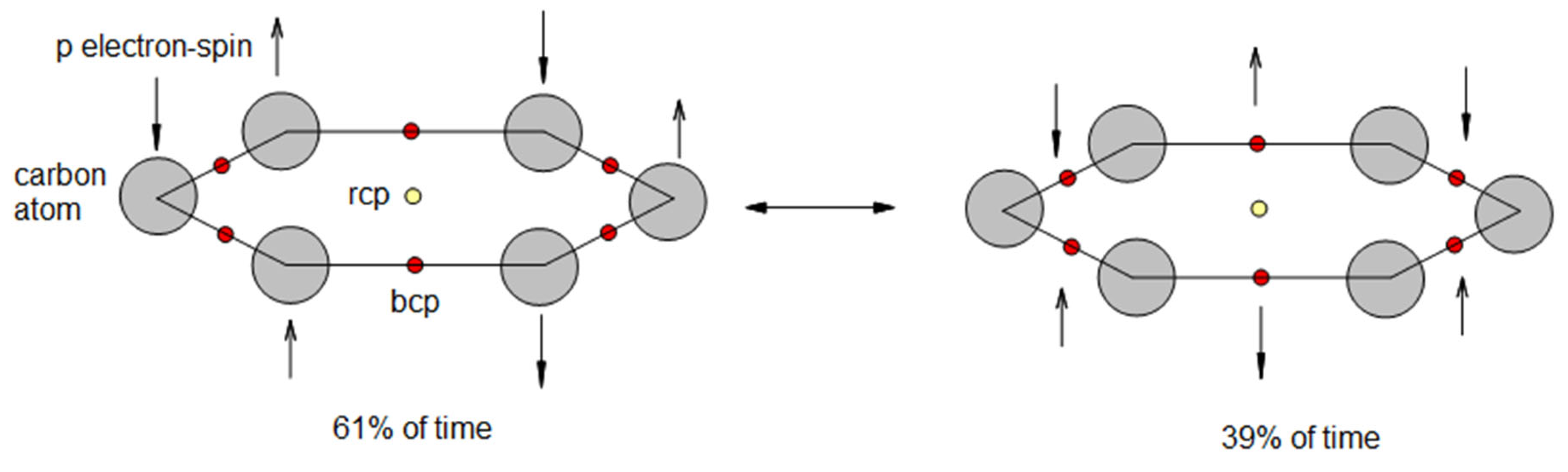

Table 1.
Ring position, ring type, delocalization index uniformity, DIU, effective π amplitude sum at ring center distance r₀ = 1.20 Å, e(∑,1.20), ρ_center, the e squared amplitude, and discrete aromaticity index D2BIA_discrete for individual rings in benzene through tetracene, calculated using the initial model with fixed 0.5 fused-bond sharing.
| Molecule | Ring (position) | Type | DIU | e(∑,1.20) | ρ_center = e² | D2BIA = DIU·ρ |
|---|---|---|---|---|---|---|
| Benzene | 1 | unique | 1.0000 | 0.15054 | 0.02266 | 0.02266 |
| Naphthalene | 1 | equivalent | 0.9167 | 0.137995 | 0.01904 | 0.01746 |
| Naphthalene | 2 | equivalent | 0.9167 | 0.137995 | 0.01904 | 0.017456 |
| Anthracene | 1 | terminal | 0.9167 | 0.137995 | 0.01904 | 0.017456 |
| Anthracene | 2 | central | 0.8333 | 0.12545 | 0.01574 | 0.01311 |
| Anthracene | 3 | terminal | 0.9167 | 0.137995 | 0.01904 | 0.017456 |
| Tetracene | 1 | terminal | 0.9167 | 0.137995 | 0.01904 | 0.017456 |
| Tetracene | 2 | internal | 0.8333 | 0.12545 | 0.01574 | 0.01311 |
| Tetracene | 3 | internal | 0.8333 | 0.12545 | 0.01574 | 0.01311 |
| Tetracene | 4 | terminal | 0.9167 | 0.13799 | 0.01904 | 0.017456 |
Table 2.
D2BIA_discrete model 1, weight, w(n), and D2BIA after refinement, model 2, of benzene to pentacene.
Table 2.
D2BIA_discrete model 1, weight, w(n), and D2BIA after refinement, model 2, of benzene to pentacene.
| Molecule | Ring (position) | Type | D2BIA (model 1) | Weight w(n) | D2BIA (with weight) |
|---|---|---|---|---|---|
| Benzene | 1 | unique | 0.02266 | 1.0000 | 0.02267 |
| Naphthalene | 1 | equivalent | 0.01746 | 0.8333 | 0.01455 |
| Naphthalene | 2 | equivalent | 0.01746 | 0.8333 | 0.01455 |
| Anthracene | 1 | terminal | 0.01746 | 0.7778 | 0.01358 |
| Anthracene | 2 | central | 0.01311 | 0.7778 | 0.01020 |
| Anthracene | 3 | terminal | 0.01746 | 0.7778 | 0.01358 |
| Tetracene | 1 | terminal | 0.01746 | 0.7500 | 0.01309 |
| Tetracene | 2 | internal | 0.01311 | 0.7500 | 0.00984 |
| Tetracene | 3 | internal | 0.01311 | 0.7500 | 0.00984 |
| Tetracene | 4 | terminal | 0.01746 | 0.7500 | 0.01309 |
| Pentacene | 1 | terminal | 0.01746 | 0.7333 | 0.01280 |
| Pentacene | 2 | internal | 0.01311 | 0.7333 | 0.00962 |
| Pentacene | 3 | central | 0.01311 | 0.7333 | 0.00962 |
| Pentacene | 4 | internal | 0.01311 | 0.7333 | 0.00962 |
| Pentacene | 5 | terminal | 0.01746 | 0.7333 | 0.01280 |
Table 3.
Ring-ID, number of rings, n, number of π electrons, N-pi, FLU_real, p, f_formula, and d_formula of each ring of 1-acene to 11-acene.
Table 3.
Ring-ID, number of rings, n, number of π electrons, N-pi, FLU_real, p, f_formula, and d_formula of each ring of 1-acene to 11-acene.
| molecule | ring_id | n | N_pi | FLU_real | P | f_formula | d_formula |
|---|---|---|---|---|---|---|---|
| Benzene | A1 | 1 | 6 | 0.00024 | 1 | 0 | 0 |
| Naphthalene | A1 | 2 | 10 | 0.01097 | 1 | 1 | 0 |
| Naphthalene | A2 | 2 | 10 | 0.01097 | 2 | 1 | 0 |
| Anthracene | A1 | 3 | 14 | 0.01609 | 1 | 1 | 0 |
| Anthracene | B | 3 | 14 | 0.01478 | 2 | 2 | 1 |
| Anthracene | A2 | 3 | 14 | 0.01609 | 3 | 1 | 0 |
| Tetracene | A1 | 4 | 18 | 0.01875 | 1 | 1 | 0 |
| Tetracene | B1 | 4 | 18 | 0.01727 | 2 | 2 | 1 |
| Tetracene | B2 | 4 | 18 | 0.01727 | 3 | 2 | 1 |
| Tetracene | A2 | 4 | 18 | 0.01875 | 4 | 1 | 0 |
| Pentacene | A1 | 5 | 22 | 0.02015 | 1 | 1 | 0 |
| Pentacene | B1 | 5 | 22 | 0.01888 | 2 | 2 | 1 |
| Pentacene | C | 5 | 22 | 0.01851 | 3 | 2 | 2 |
| Pentacene | B2 | 5 | 22 | 0.01888 | 4 | 2 | 1 |
| Pentacene | A2 | 5 | 22 | 0.02015 | 5 | 1 | 0 |
| Hexacene | A1 | 6 | 26 | 0.02092 | 1 | 1 | 0 |
| Hexacene | B1 | 6 | 26 | 0.01981 | 2 | 2 | 1 |
| Hexacene | C1 | 6 | 26 | 0.01953 | 3 | 2 | 2 |
| Hexacene | C2 | 6 | 26 | 0.01953 | 4 | 2 | 2 |
| Hexacene | B2 | 6 | 26 | 0.01981 | 5 | 2 | 1 |
| Hexacene | A2 | 6 | 26 | 0.02092 | 6 | 1 | 0 |
| Heptacene | A1 | 7 | 30 | 0.02134 | 1 | 1 | 0 |
| Heptacene | B1 | 7 | 30 | 0.02034 | 2 | 2 | 1 |
| Heptacene | C1 | 7 | 30 | 0.02018 | 3 | 2 | 2 |
| Heptacene | D | 7 | 30 | 0.02025 | 4 | 2 | 3 |
| Heptacene | C2 | 7 | 30 | 0.02018 | 5 | 2 | 2 |
| Heptacene | B2 | 7 | 30 | 0.02034 | 6 | 2 | 1 |
| Heptacene | A2 | 7 | 30 | 0.02134 | 7 | 1 | 0 |
| Octacene | A1 | 8 | 34 | 0.02157 | 1 | 1 | 0 |
| Octacene | B1 | 8 | 34 | 0.02065 | 2 | 2 | 1 |
| Octacene | C1 | 8 | 34 | 0.02056 | 3 | 2 | 2 |
| Octacene | D1 | 8 | 34 | 0.02073 | 4 | 2 | 3 |
| Octacene | D2 | 8 | 34 | 0.02073 | 5 | 2 | 3 |
| Octacene | C2 | 8 | 34 | 0.02056 | 6 | 2 | 2 |
| Octacene | B2 | 8 | 34 | 0.02065 | 7 | 2 | 1 |
| Octacene | A2 | 8 | 34 | 0.02157 | 8 | 1 | 0 |
| Nonacene | A1 | 9 | 38 | 0.02171 | 1 | 1 | 0 |
| Nonacene | B1 | 9 | 38 | 0.02083 | 2 | 2 | 1 |
| Nonacene | C1 | 9 | 38 | 0.02079 | 3 | 2 | 2 |
| Nonacene | D1 | 9 | 38 | 0.02104 | 4 | 2 | 3 |
| Nonacene | E | 9 | 38 | 0.02113 | 5 | 2 | 4 |
| Nonacene | D2 | 9 | 38 | 0.02104 | 6 | 2 | 3 |
| Nonacene | C2 | 9 | 38 | 0.02079 | 7 | 2 | 2 |
| Nonacene | B2 | 9 | 38 | 0.02083 | 8 | 2 | 1 |
| Nonacene | A2 | 9 | 38 | 0.02171 | 9 | 1 | 0 |
| Decacene | A1 | 10 | 42 | 0.02179 | 1 | 1 | 0 |
| Decacene | B1 | 10 | 42 | 0.02093 | 2 | 2 | 1 |
| Decacene | C1 | 10 | 42 | 0.02093 | 3 | 2 | 2 |
| Decacene | D1 | 10 | 42 | 0.02122 | 4 | 2 | 3 |
| Decacene | E1 | 10 | 42 | 0.02139 | 5 | 2 | 4 |
| Decacene | E2 | 10 | 42 | 0.02139 | 6 | 2 | 4 |
| Decacene | D2 | 10 | 42 | 0.02122 | 7 | 2 | 3 |
| Decacene | C2 | 10 | 42 | 0.02093 | 8 | 2 | 2 |
| Decacene | B2 | 10 | 42 | 0.02093 | 9 | 2 | 1 |
| Decacene | A2 | 10 | 42 | 0.02179 | 10 | 1 | 0 |
| Undecacene | A1 | 11 | 46 | 0.02184 | 1 | 1 | 0 |
| Undecacene | B1 | 11 | 46 | 0.02099 | 2 | 2 | 1 |
| Undecacene | C1 | 11 | 46 | 0.021 | 3 | 2 | 2 |
| Undecacene | D1 | 11 | 46 | 0.02133 | 4 | 2 | 3 |
| Undecacene | E1 | 11 | 46 | 0.02154 | 5 | 2 | 4 |
| Undecacene | F | 11 | 46 | 0.02162 | 6 | 2 | 5 |
| Undecacene | E2 | 11 | 46 | 0.02154 | 7 | 2 | 4 |
| Undecacene | D2 | 11 | 46 | 0.02133 | 8 | 2 | 3 |
| Undecacene | C2 | 11 | 46 | 0.021 | 9 | 2 | 2 |
| Undecacene | B2 | 11 | 46 | 0.02099 | 10 | 2 | 1 |
| Undecacene | A2 | 11 | 46 | 0.02184 | 11 | 1 | 0 |
Table 4.
11-Fold LONOCV metrics (train and test R2, RMSE, and MRE%) of model 3 for 1-acene to 11-acene (where alpha = 1 and gamma = 0.05 for all 11-fold CVs).
Table 4.
11-Fold LONOCV metrics (train and test R2, RMSE, and MRE%) of model 3 for 1-acene to 11-acene (where alpha = 1 and gamma = 0.05 for all 11-fold CVs).
| left_out_n | train_R2 | train_RMSE | train_MRE_% | test_R2 | test_RMSE | test_MRE_% | n_train_points |
|---|---|---|---|---|---|---|---|
| 1 | 0.4409 | 0.001625 | 6.69 | 0.011992 | 4996.74 | 65 | |
| 2 | 0.5445 | 0.001951 | 67.78 | 0.003955 | 36.05 | 64 | |
| 3 | 0.5915 | 0.002038 | 63.00 | -6.02461 | 0.001637 | 7.21 | 63 |
| 4 | 0.6154 | 0.002053 | 61.04 | -2.65014 | 0.001414 | 7.67 | 62 |
| 5 | 0.6322 | 0.002042 | 60.80 | -5.33535 | 0.001751 | 6.85 | 61 |
| 6 | 0.6382 | 0.002044 | 61.36 | -7.96264 | 0.001797 | 7.17 | 60 |
| 7 | 0.6418 | 0.002045 | 61.98 | -12.672 | 0.001821 | 7.16 | 59 |
| 8 | 0.6405 | 0.002058 | 62.87 | -17.5965 | 0.001744 | 6.74 | 58 |
| 9 | 0.6422 | 0.002061 | 62.91 | -24.9173 | 0.001772 | 6.93 | 57 |
| 10 | 0.6426 | 0.002067 | 62.80 | -29.8499 | 0.001786 | 7.12 | 56 |
| 11 | 0.6523 | 0.002046 | 60.77 | -38.5461 | 0.002013 | 8.11 | 55 |
Table 5.
Average D2BIA_discrete from models 1 and 2 along with global values of FLU, PDI, HOMA and NICS(1)_zz from 1-acene (benzene) to 10-acene (decacene).
Table 5.
Average D2BIA_discrete from models 1 and 2 along with global values of FLU, PDI, HOMA and NICS(1)_zz from 1-acene (benzene) to 10-acene (decacene).
| N | Molecule | D2BIA_Model1 | D2BIA_Model2 | FLU | PDI | HOMA | NICS(1)_ZZ |
|---|---|---|---|---|---|---|---|
| 1 | Benzene | 0.02266 | 0.02266 | 0.00024 | 0.11598 | 0.971 | -28.85 |
| 2 | Naphthalene | 0.01746 | 0.01455 | 0.01097 | 0.09144 | 0.748 | -28.84 |
| 3 | Anthracene | 0.01601 | 0.01245 | 0.01565 | 0.08312 | 0.617 | -28.75 |
| 4 | Tetracene | 0.01529 | 0.01146 | 0.01801 | 0.07943 | 0.538 | -28.84 |
| 5 | Pentacene | 0.01485 | 0.01089 | 0.01931 | 0.07757 | 0.489 | -29.01 |
| 6 | Hexacene | 0.01456 | 0.01052 | 0.02008 | 0.07657 | 0.457 | -29.23 |
| 7 | Heptacene | 0.01436 | 0.01025 | 0.02056 | 0.0760 | 0.436 | -29.46 |
| 8 | Octacene | 0.01420 | 0.01006 | 0.02088 | 0.07567 | 0.421 | -29.69 |
| 9 | Nonacene | 0.01408 | 0.00991 | 0.0211 | 0.07546 | 0.410 | -29.91 |
| 10 | Decacene | 0.01398 | 0.00979 | 0.02125 | 0.07534 | 0.402 | -30.12 |
Table 6.
Coefficient of determination, R2, and corresponding equation for linear, logarithmic, power, and exponential relations of D2BIA_discrete models 1 and 2 with FLU, PDI, HOMA, and NICS(1)_zz for 1-acene to 10-acene.
Table 6.
Coefficient of determination, R2, and corresponding equation for linear, logarithmic, power, and exponential relations of D2BIA_discrete models 1 and 2 with FLU, PDI, HOMA, and NICS(1)_zz for 1-acene to 10-acene.
| Model | Index | Fit_Type | R² | Equation |
|---|---|---|---|---|
| Model1 | FLU | Linear | 0.9911 | y = -2.490659*x + 0.056019 |
| Model1 | FLU | Logarithmic | 0.9971 | y = -0.044658*ln(x) + -0.169067 |
| Model1 | FLU | Power | 0.8913 | y = 0.000000*x^-8.806870 |
| Model1 | FLU | Exponential | 0.9291 | y = 32.627114*exp(-502.986989*x) |
| Model1 | PDI | Linear | 0.9966 | y = 4.787968*x + 0.007275 |
| Model1 | PDI | Logarithmic | 0.9887 | y = 0.085253*ln(x) + 0.437488 |
| Model1 | PDI | Power | 0.9948 | y = 3.702554*x^0.915682 |
| Model1 | PDI | Exponential | 0.9953 | y = 0.036562*exp(51.234032*x) |
| Model1 | HOMA | Linear | 0.9524 | y = 67.614466*x + -0.515638 |
| Model1 | HOMA | Logarithmic | 0.9764 | y = 1.223820*ln(x) + 5.642537 |
| Model1 | HOMA | Power | 0.9295 | y = 1421.962744*x^1.898501 |
| Model1 | HOMA | Exponential | 0.8915 | y = 0.102341*exp(104.008138*x) |
| Model1 | NICS(1)_ZZ | Linear | 0.3245 | y = 106.807366*x + -30.951600 |
| Model1 | NICS(1)_ZZ | Logarithmic | 0.3764 | y = 2.056115*ln(x) + -20.712288 |
| Model2 | FLU | Linear | 0.9845 | y = -1.673918*x + 0.037317 |
| Model2 | FLU | Logarithmic | 0.9976 | y = -0.025618*ln(x) + -0.096853 |
| Model2 | FLU | Power | 0.8835 | y = 0.000000*x^-5.028614 |
| Model2 | FLU | Exponential | 0.9461 | y = 0.786902*exp(-342.285959*x) |
| Model2 | PDI | Linear | 0.9974 | y = 3.230054*x + 0.043077 |
| Model2 | PDI | Logarithmic | 0.9868 | y = 0.048844*ln(x) + 0.299363 |
| Model2 | PDI | Power | 0.9943 | y = 0.841209*x^0.524985 |
| Model2 | PDI | Exponential | 0.9921 | y = 0.053675*exp(34.494417*x) |
| Model2 | HOMA | Linear | 0.9362 | y = 45.206642*x + -0.005059 |
| Model2 | HOMA | Logarithmic | 0.9800 | y = 0.703146*ln(x) + 3.668551 |
| Model2 | HOMA | Power | 0.9354 | y = 66.953706*x^1.092233 |
| Model2 | HOMA | Exponential | 0.8680 | y = 0.225377*exp(69.207561*x) |
| Model2 | NICS(1)_ZZ | Linear | 0.2959 | y = 68.771643*x + -30.112723 |
| Model2 | NICS(1)_ZZ | Logarithmic | 0.3835 | y = 1.190366*ln(x) + -23.988693 |
Table 7.
Real FLU and SCI values from literature, D2BIA_discrete (LONOCV Model 3) and corresponding predicted FLU, FLU_pred, from all rings of 1-acene to 11-acene.
Table 7.
Real FLU and SCI values from literature, D2BIA_discrete (LONOCV Model 3) and corresponding predicted FLU, FLU_pred, from all rings of 1-acene to 11-acene.
| Molecule | Ring | FLU_real | D2BIA_discrete | FLU_pred | SCI(×10²) |
|---|---|---|---|---|---|
| Benzene | A1 | 0.00024 | 0.02266 | 0.01223 | 7.685 |
| Naphthalene | A1 | 0.01097 | 0.01889 | 0.01493 | 4.503 |
| Naphthalene | A2 | 0.01097 | 0.01889 | 0.01493 | 4.503 |
| Anthracene | A1 | 0.01609 | 0.01763 | 0.01629 | 3.530 |
| Anthracene | B | 0.01478 | 0.01677 | 0.01760 | 3.363 |
| Anthracene | A2 | 0.01609 | 0.01763 | 0.01629 | 3.530 |
| Tetracene | A1 | 0.01875 | 0.01700 | 0.01710 | 3.097 |
| Tetracene | B1 | 0.01727 | 0.01617 | 0.01840 | 2.898 |
| Tetracene | B2 | 0.01727 | 0.01617 | 0.01840 | 2.898 |
| Tetracene | A2 | 0.01875 | 0.01700 | 0.01710 | 3.097 |
| Pentacene | A1 | 0.02015 | 0.01662 | 0.01763 | 2.886 |
| Pentacene | B1 | 0.01888 | 0.01581 | 0.01892 | 2.648 |
| Pentacene | C | 0.01851 | 0.01504 | 0.02014 | 2.610 |
| Pentacene | B2 | 0.01888 | 0.01581 | 0.01892 | 2.648 |
| Pentacene | A2 | 0.02015 | 0.01662 | 0.01763 | 2.886 |
| Hexacene | A1 | 0.02092 | 0.01637 | 0.01801 | 2.777 |
| Hexacene | B1 | 0.01981 | 0.01557 | 0.01928 | 2.513 |
| Hexacene | C1 | 0.01953 | 0.01481 | 0.02048 | 2.438 |
| Hexacene | C2 | 0.01953 | 0.01481 | 0.02048 | 2.438 |
| Hexacene | B2 | 0.01981 | 0.01557 | 0.01928 | 2.513 |
| Hexacene | A2 | 0.02092 | 0.01637 | 0.01801 | 2.777 |
| Heptacene | A1 | 0.02134 | 0.01619 | 0.01829 | 2.717 |
| Heptacene | B1 | 0.02034 | 0.01540 | 0.01955 | 2.440 |
| Heptacene | C1 | 0.02018 | 0.01465 | 0.02075 | 2.339 |
| Heptacene | D | 0.02025 | 0.01393 | 0.02189 | 2.304 |
| Heptacene | C2 | 0.02018 | 0.01465 | 0.02075 | 2.339 |
| Heptacene | B2 | 0.02034 | 0.01540 | 0.01955 | 2.440 |
| Heptacene | A2 | 0.02134 | 0.01619 | 0.01829 | 2.717 |
| Octacene | A1 | 0.02157 | 0.01605 | 0.01851 | 2.684 |
| Octacene | B1 | 0.02065 | 0.01527 | 0.01976 | 2.399 |
| Octacene | C1 | 0.02056 | 0.01453 | 0.02095 | 2.283 |
| Octacene | D1 | 0.02073 | 0.01382 | 0.02208 | 2.224 |
| Octacene | D2 | 0.02073 | 0.01382 | 0.02208 | 2.224 |
| Octacene | C2 | 0.02056 | 0.01453 | 0.02095 | 2.283 |
| Octacene | B2 | 0.02065 | 0.01527 | 0.01976 | 2.399 |
| Octacene | A2 | 0.02157 | 0.01605 | 0.01851 | 2.684 |
| Nonacene | A1 | 0.02171 | 0.01595 | 0.01869 | 2.665 |
| Nonacene | B1 | 0.02083 | 0.01517 | 0.01995 | 2.375 |
| Nonacene | C1 | 0.02079 | 0.01443 | 0.02116 | 2.251 |
| Nonacene | D1 | 0.02104 | 0.01373 | 0.02230 | 2.178 |
| Nonacene | E | 0.02113 | 0.01306 | 0.02338 | 2.154 |
| Nonacene | D2 | 0.02104 | 0.01373 | 0.02230 | 2.178 |
| Nonacene | C2 | 0.02079 | 0.01443 | 0.02116 | 2.251 |
| Nonacene | B2 | 0.02083 | 0.01517 | 0.01995 | 2.375 |
| Nonacene | A2 | 0.02171 | 0.01595 | 0.01869 | 2.665 |
| Decacene | A1 | 0.02179 | 0.01586 | 0.01885 | 2.654 |
| Decacene | B1 | 0.02093 | 0.01509 | 0.02013 | 2.362 |
| Decacene | C1 | 0.02093 | 0.01435 | 0.02134 | 2.233 |
| Decacene | D1 | 0.02122 | 0.01365 | 0.02250 | 2.152 |
| Decacene | E1 | 0.02139 | 0.01299 | 0.02360 | 2.114 |
| Decacene | E2 | 0.02139 | 0.01299 | 0.02360 | 2.114 |
| Decacene | D2 | 0.02122 | 0.01365 | 0.02250 | 2.152 |
| Decacene | C2 | 0.02093 | 0.01435 | 0.02134 | 2.233 |
| Decacene | B2 | 0.02093 | 0.01509 | 0.02013 | 2.362 |
| Decacene | A2 | 0.02179 | 0.01586 | 0.01885 | 2.654 |
| Undecacene | A1 | 0.02184 | 0.01580 | 0.01901 | 2.648 |
| Undecacene | B1 | 0.02099 | 0.01503 | 0.02033 | 2.354 |
| Undecacene | C1 | 0.02100 | 0.01429 | 0.02159 | 2.222 |
| Undecacene | D1 | 0.02133 | 0.01360 | 0.02278 | 2.136 |
| Undecacene | E1 | 0.02154 | 0.01293 | 0.02392 | 2.090 |
| Undecacene | F | 0.02162 | 0.01230 | 0.02500 | 2.076 |
| Undecacene | E2 | 0.02154 | 0.01293 | 0.02392 | 2.090 |
| Undecacene | D2 | 0.02133 | 0.01360 | 0.02278 | 2.136 |
| Undecacene | C2 | 0.02100 | 0.01429 | 0.02159 | 2.222 |
| Undecacene | B2 | 0.02099 | 0.01503 | 0.02033 | 2.354 |
| Undecacene | A2 | 0.02184 | 0.01580 | 0.01901 | 2.648 |
Disclaimer/Publisher’s Note: The statements, opinions and data contained in all publications are solely those of the individual author(s) and contributor(s) and not of MDPI and/or the editor(s). MDPI and/or the editor(s) disclaim responsibility for any injury to people or property resulting from any ideas, methods, instructions or products referred to in the content. |
© 2026 by the authors. Licensee MDPI, Basel, Switzerland. This article is an open access article distributed under the terms and conditions of the Creative Commons Attribution (CC BY) license (http://creativecommons.org/licenses/by/4.0/).
Copyright: This open access article is published under a Creative Commons CC BY 4.0 license, which permit the free download, distribution, and reuse, provided that the author and preprint are cited in any reuse.


