
Submitted:
20 January 2025
Posted:
21 January 2025
You are already at the latest version
Abstract
Topological indices characterize the molecular structure of a graph and are called numerical parameters used to estimate physicochemical information. In this article, firstly the Euler Sombor coindex and Gourava Sombor coindex are introduced. Then, bounds for Euler Sombor and Gourava Sombor coindices depending on some other coindices were obtained and bounds in terms of minimum degree, maximum degree, order and size of the graphs are computed for these indices of several graph operations. Next, Euler Sombor coindex and Gourava Sombor coindex of some chemical graphs such as polyamidoamine, graphene, carbon nanocones and caterpillar are studied. Finally, by developing a nonlinear regression model using the QSPR approach and utilizing the Euler Sombor and Gourava Sombor indices and their coindices, the physicochemical properties of interest of butane derivatives were predicted. The results showed that these indices have satisfactory performance in comparative tests.
Keywords:
Chemical graph
; Topological index
; Euler Sombor index
; Gourava Sombor index
; QSPR analysis
MSC: 05C07; 05C09; 05C92
1. Introduction
Consider a simply connected graph, denoted , whose vertices and edge sets are and , respectively. The graph , whose set of vertices is the same as the Ѵ(S) and set of edges is () is the complement of . For other graph-theoretical notation and terminology, we refer to [1,2].
In this article, will be considered as a simple connected graph with edges and vertices. The degree of the vertices in this graph is , where ∆ and δ denote the maximum and minimum degrees, respectively.
Topological indices are among the prominent subjects of Graph Theory. Chemical graph theory generally considers various topological indices (molecular descriptors) of molecular graphs and examines how strongly they are related to various properties of the corresponding molecules. Thus, mathematical representations of these relationships are obtained with QSAR and QSPR studies in the literature.
There are studies in the literature on topological indices and coindices [3,4,5,6,7,8,9,10,11,12,13,14,15,16,17,18]. In Table 1, we give some degree based topological indices and coindices.
In the light of these definitions, Euler Sombor and Gourava Sombor co-indices defined as
and
The bounds for Euler Sombor and Gourava Sombor co-indices depending on the Zagreb coindices, Hyper Zagreb coindices and forgetten topological coindex were obtained. The bounds are computed for these indices of several graph operations like union, sum, cartesian product and composition of graphs [25]. Euler Sombor coindex and Gourava Sombor coindex of some chemical graphs are studied. An analysis of the physicochemical properties of butane and its derivatives was performed to evaluate the effects of Euler Sombor and Gourava Sombor indices and co-indices in QSPR studies. A non-linear model was developed using the QSPR approach to predict the specified properties and the results showed that the indices have satisfactory performance in comparative tests in predicting all the properties.
2. The Euler Sombor and Gourava Sombor Coindices
In this section, the bounds for Euler Sombor and Gourava Sombor coindices depending on the Zagreb coindices, Hyper Zagreb coindices and forgetten topological coindex were obtained. The bounds are computed for these indices of the graph operations like union, sum, cartesian product and composition of graphs.
2.1. Bounds for Euler Sombor Coindex and Gourava Sombor Coindex Depending on Some Other Topological Coindices
First, let's give the necessary inequalities for the obtained results.
Lemma 2.1.1.
(P´olya-Szegö Inequality [26])
Let , , … and , , … be two sequences of positive real numbers. If there exists real numbers , , and such that and for then
Lemma 2.1.2.
(Radon’s inequality [26])
If for and ,
Theorem 2.1.3.
Let be a graph on vertices and edges. Then
Proof.
Letting and in Lemma 2.1.1, and choosing
and , we get and for Applying Lemma 2.1.1 with the sums running over the edges in , we have
Using the definitions of Forgetten and Second Zagreb coindices, we get
Hence we obtain the lower bound as
For the upper bound, letting and in Lemma 2.1.2 with the sums running over the edges in , we have
Notice that
Thus, we get
Theorem 2.1.4.
Let be a graph on vertices and edges. Then
Proof.
Letting and in Lemma 2.1.1, and choosing and , we get and for Applying Lemma 2.1.1 with the sums running over the edges in , we get
Using the definitions of Hyper Zagreb coindices, we have
For the upper bound, letting and in Lemma 2.1.2 with the sums running over the edges in , we have
Notice that
Hence, we get
2.2. Bounds on the Euler Sombor Coindex and Gourava Sombor Coindex of Graph Operations
In this section, the minimum degree of the graph ) will be taken as and the maximum degree will be taken as .
Theorem 2.2.1.
Let and be two graphs on and vertices, respectively. Then, the the union of the graphs and on the Euler Sombor coindex has the lower and upper bounds as
Moreover, the equality holds if and are regular.
Proof.
By the definition of Euler Sombor coindex, we have
Using the minimum and maximum degrees, we obtain the desired result.
Theorem 2.2.2.
Let and be two graphs on and vertices, respectively. Then, the the union of the graphs and on the Gourava Sombor coindex has the lower and upper bounds as
Moreover, the equality holds if and are regular.
Proof.
By the definition of Gourava Sombor coindex, we have
Hence, we get the desired result.
Theorem 2.2.3.
Let and be two graphs on and vertices, and edges respectively. Then, the the sum of the graphs and on the Euler Sombor coindex has the lower and upper bounds as
Here, the number of edges of the graph for i=1,2 is . Moreover, the equality holds if and are regular.
Proof.
By the definition of Euler Sombor coindex, we get
Using the definition of the sum of two graphs, we get
Using the minimum and maximum degrees, we obtain
Theorem 2.2.4.
Let and be two graphs on and vertices, and edges respectively. Then, the the sum of the graphs and on the Gourava Sombor coindex has the lower and upper bounds as
Here, the number of edges of the graph for i=1,2 is . Moreover, the equality holds if and are regular.
Proof.
By the definition of Gourava Sombor coindex, we have
Using the definition of the sum of two graphs, we get
Using the minimum and maximum degrees, we get the desired result.
Theorem 2.2.5.
Let and be two graphs on and vertices, and edges respectively. Then, the cartesian product of the graphs and on the Euler Sombor coindex has the lower and upper bounds as
dir. Here, the number of edges of the graph is .
Proof.
Let and . By the definition of Euler Sombor coindex, we have
Hence, we get the desired bounds.
Theorem 2.2.6.
Let and be two graphs on and vertices, and edges respectively. Then, the the cartesian product of the graphs and on the Gourava Sombor coindex has the lower and upper bounds as
Here, the number of edges of the graph is .
Proof.
Let and . By the definition of Gourava Sombor coindex, we have
Hence, we get
Theorem 2.2.7.
Let and be two graphs on and vertices, and edges respectively. Then, the the composition of the graphs and on the Euler Sombor coindex has the lower and upper bounds as
Here, the number of edges of the graph is
Proof.
Let and . By the definition of Euler Sombor coindex, we get
Hence, we obtain
Theorem 2.2.8.
Let and be two graphs on and vertices, and edges respectively. Then, the the composition of the graphs and on the Gourava Sombor coindex has the lower and upper bounds as
Here, the number of edges of the graph is
Proof.
Let and . By the definition of Gourava Sombor coindex, we get
Hence, we get the desired bounds.
3. The Euler Sombor and Gourava Sombor Coindices of SOME chemical Graphs
is a chemical graph if for all . We denote by the number of vertices of degree . Let and be the number of adjacent and non-adjacent vertex of degree to a vertex of degree respectively. Here, and , for
Proposition 3.1. If is a chemical graph, then the Euler Sombor coindex and the Gourava Sombor coindex are are as follows respectively:
and
Proof. For a chemical graph , there exist only type of vertex pairs. Using the definitions of the Euler and Gourava coindices, the desired result can be get easily.
Dendrimer has a special structure that is generally divided into three parts: inner layer, middle layer and surface functional group layer. If the molecular graph of porphyrin core polyamidoamine dendrimers synthesized by microwave method[27] is shown with PDP(k), where is the production step, the following theorem is obtained.
Theorem 3.2. Let . Then the Euler and Gourava coindices of PDP(k) are
and
where
Then the Euler and Gourava coindices of PDP(k) are
Graphene is a material with a two-dimensional honeycomb lattice structure consisting of a single layer of atoms and is denoted by .
Theorem 3.3. Let be the graphene where Then the Euler and Gourava coindices of are
Proof. Since has only and -type of vertex pairs, we can see easy that , and If these values are written in the equations, we obtain
and
If the necessary calculations are made, the desired results are obtained.
Carbon nanocones are conical structures with a loop of length at the core and hexagonal layers arranged on a conical surface around the center, denoted by .
Theorem 3.4. Let be the carbon nanocone structure with and Then,
Proof. It is easy to check that , If we calculate and , the desired results are obtained.
A tree is a caterpillar if and only if all vertex of degree greater than equal are surrounded by at most two vertices of degree two or greater.
Proposition 3.5. Let be the caterpillar . Then we have
and
Proof. It is seen from the structure of that and . Then we get
and
When the values of and are substituted into the equations above, the desired results are obtained.
4. The Use of Selected Sombor Topological Indices and Coindices in QSPR Studies
QSPR studies have become an important field of study for both mathematicians and chemists with the advantage of rapid calculation of topological indices to predict the properties of compounds. In this section, we have shown that Euler Sombor and Gourava Sombor indices and their coindices play an important role in the prediction of Hydrogen bond acceptor count (HBAC), Heavy atomic count (HAC), Complexity (COMP), and Surface Tension(ST) properties.

Table 2.
Experimental values of physicochemical properties of Butane derivatives [29].
Table 2.
Experimental values of physicochemical properties of Butane derivatives [29].
| Compound | HBAC | HAC | COMP | ST |
| 1,4-butanedithiol | 2 | 6 | 17.5 | 31.1 |
| 2-butanone | 1 | 5 | 38.5 | 22.9 |
| 1,3-butanediol | 2 | 6 | 28.7 | 34.9 |
| butane dinitrile | 2 | 6 | 92 | 40.7 |
| butanediamide | 2 | 8 | 96.6 | 53 |
| butane-1-sulfoamide | 3 | 8 | 133 | 41.9 |
| 1-butanethiol | 1 | 5 | 13.1 | 24.8 |
| 1,4-diaminobuane | 2 | 6 | 17.5 | 35.8 |
| butane-1,4-disulfonic acid | 6 | 12 | 266 | 77.9 |
| butyraldehyde | 1 | 5 | 24.8 | 23.1 |
| 2,3-butanedione | 2 | 6 | 71.5 | 27.3 |
| 1-butanesufonylchloride | 2 | 8 | 133 | 36.4 |
Table 3.
Gourava and Sombor indices(coindices) of Butane derivatives.
| Compound | ||||
| 1,4-butanedithiol | 24.18 | 15.68 | 27.99 | 40.83 |
| 2-butanone | 30 | 17.81 | 17.71 | 25.11 |
| 1,3-butanediol | 27.07 | 17.67 | 26.38 | 37.54 |
| butane dinitrile | 53.44 | 26.21 | 52.30 | 96.91 |
| butanediamide | 58.46 | 33.79 | 77.47 | 130.05 |
| butane-1-sulfoamide | 85.92 | 49.98 | 91.83 | 149.39 |
| 1-butanethiol | 18.52 | 17.51 | 26.36 | 22.31 |
| 1,4-diaminobuane | 24.18 | 20.97 | 27.99 | 40.83 |
| butane-1,4-disulfonic acid | 121.94 | 66.77 | 231.47 | 390.13 |
| butyraldehyde | 24.88 | 14.82 | 20.18 | 31.33 |
| 2,3-butanedione | 50.69 | 30.13 | 35.52 | 55.12 |
| 1-butanesufonylchloride | 67.40 | 37.76 | 74.23 | 118 |
- Non-linear Regression Model:
Here, we based on the below non-linear regression model:
where indicates the selected properties of Butane derivatives, and indicates the Gourava and Sombor indices(coindices).
The Gourava Sombor index :
The Euler Sombor index :
The Gourava Sombor coindex :
The Euler Sombor coindex :
When the necessary calculations are made here, it is seen that the predicted values of the properties are as in Table 4, Table 5, Table 6 and Table 7. The correlation coefficients of the experimental values and the exact values of the selected physicochemical properties of the butane derivative are given in Table 8. The values for the nonlinear QSPR model are shown in Table .
The following figures indicates how much the predicted values of physio-chemical properties are correlated with the wellknown physio-chemical properties.
Figure 1.
Graphical relationships between predicted values of HBAC and its exact values.
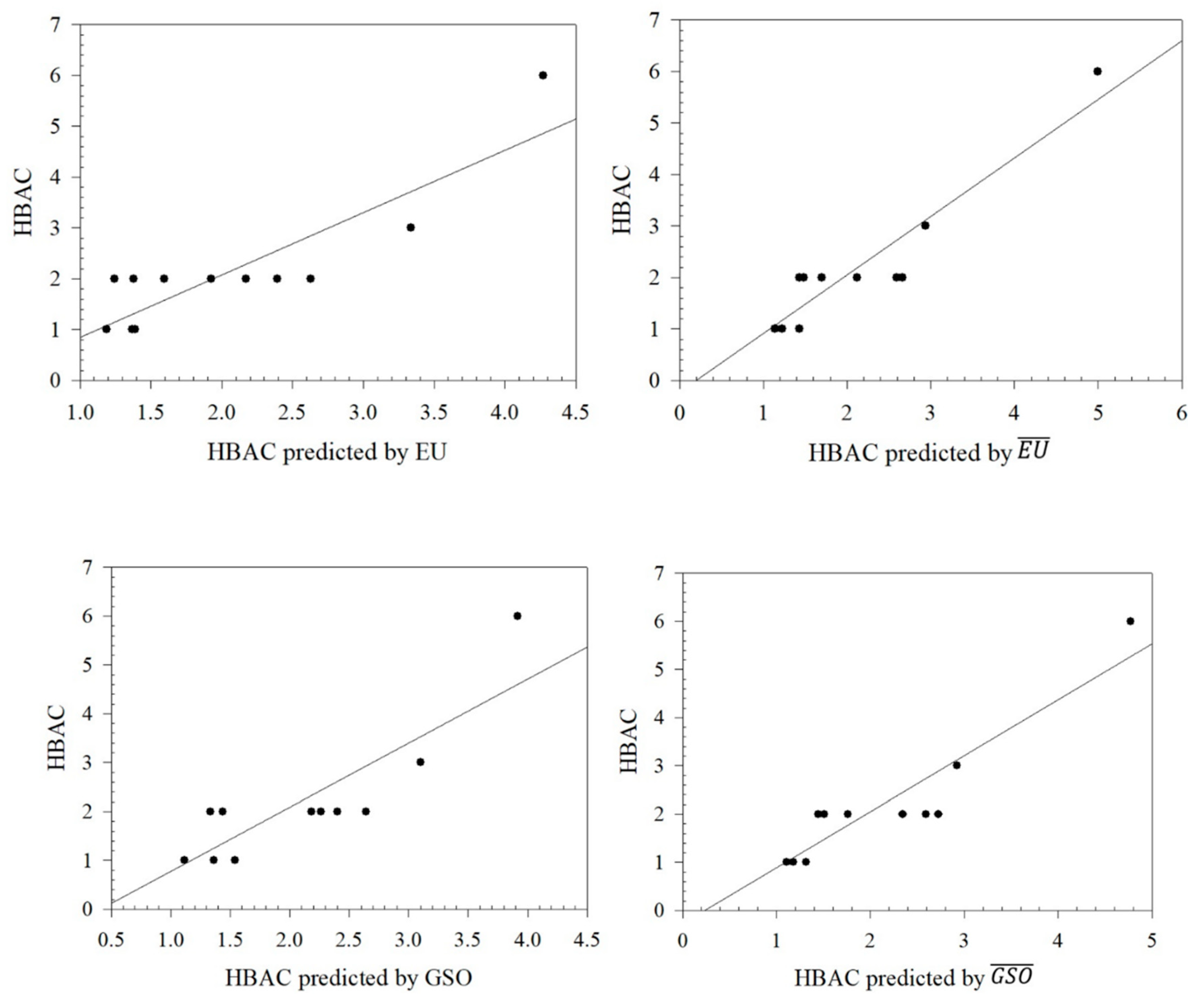
Figure 2.1.
Graphical relationships between predicted values of HAC and its exact values and .
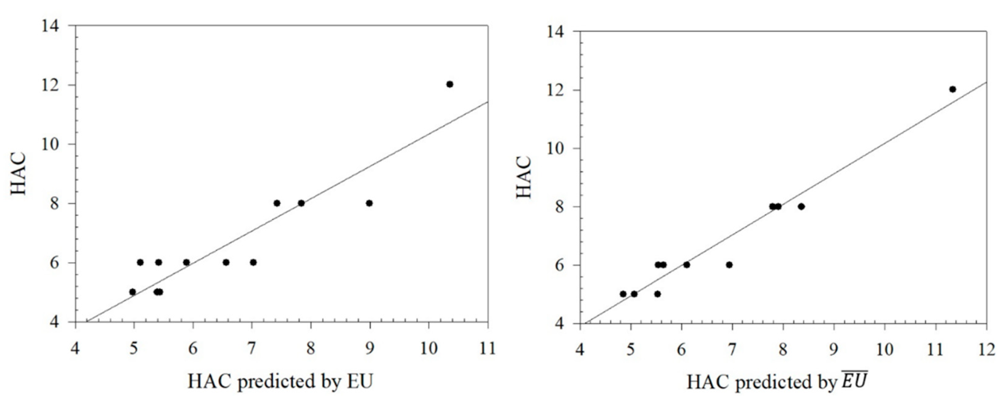
Figure 2.2.
Graphical relationships between predicted values of HAC and its exact values and .
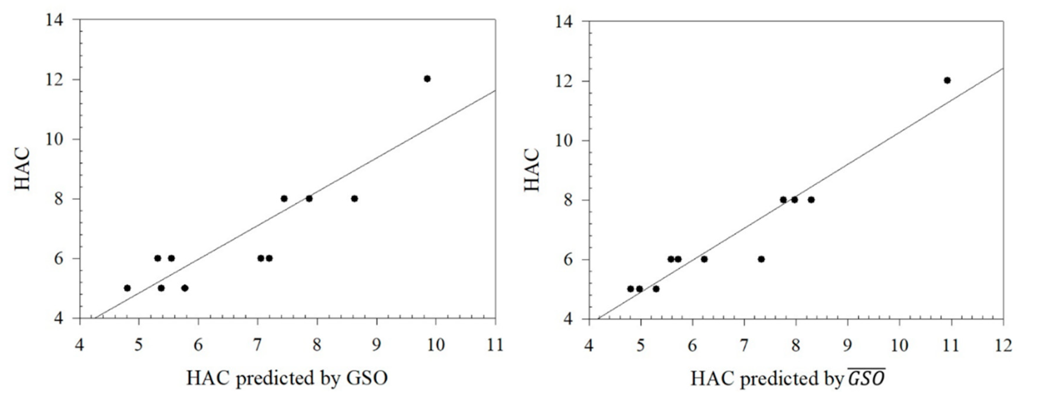
Figure 3.
Graphical relationships between predicted values of COMP and its exact values.
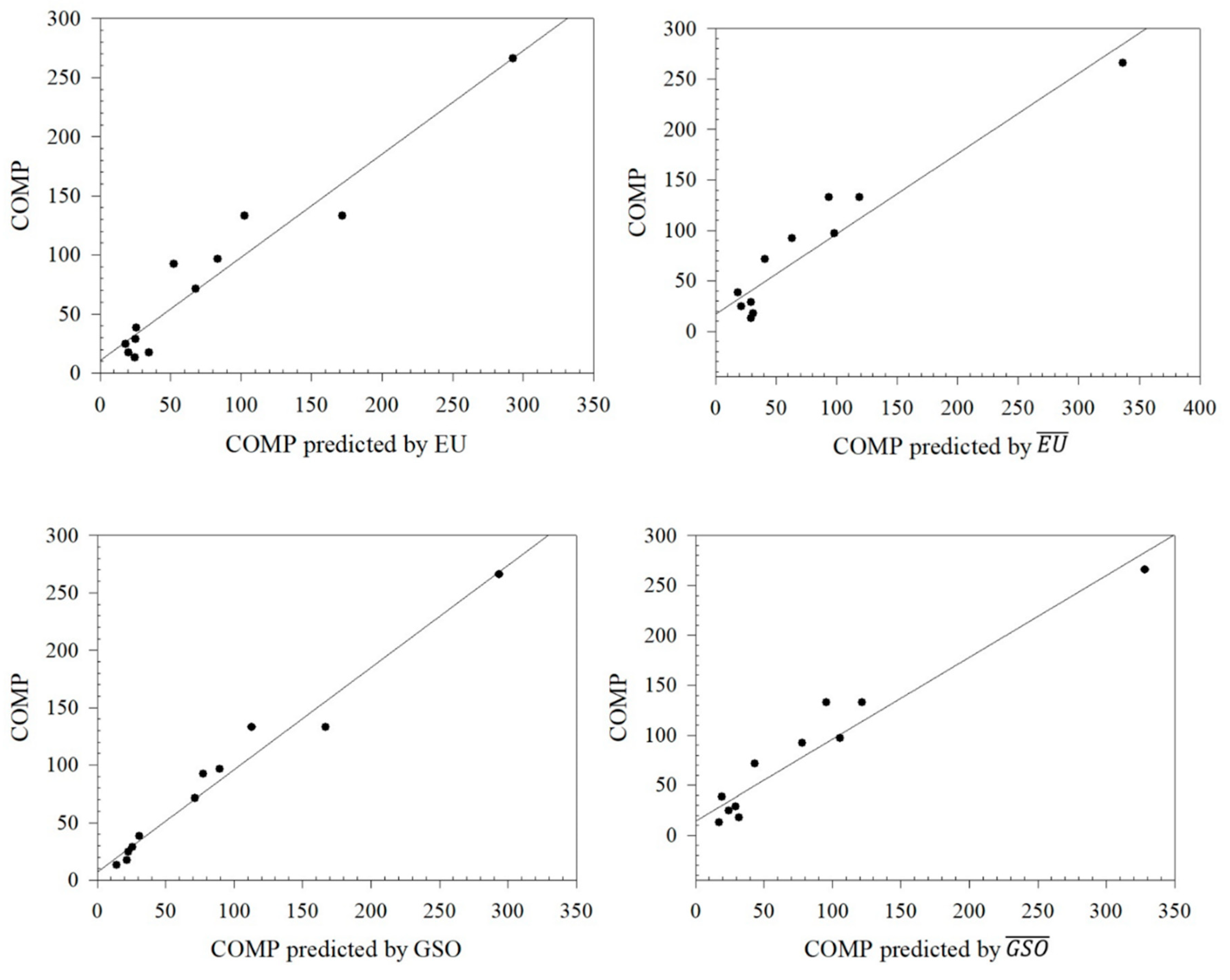
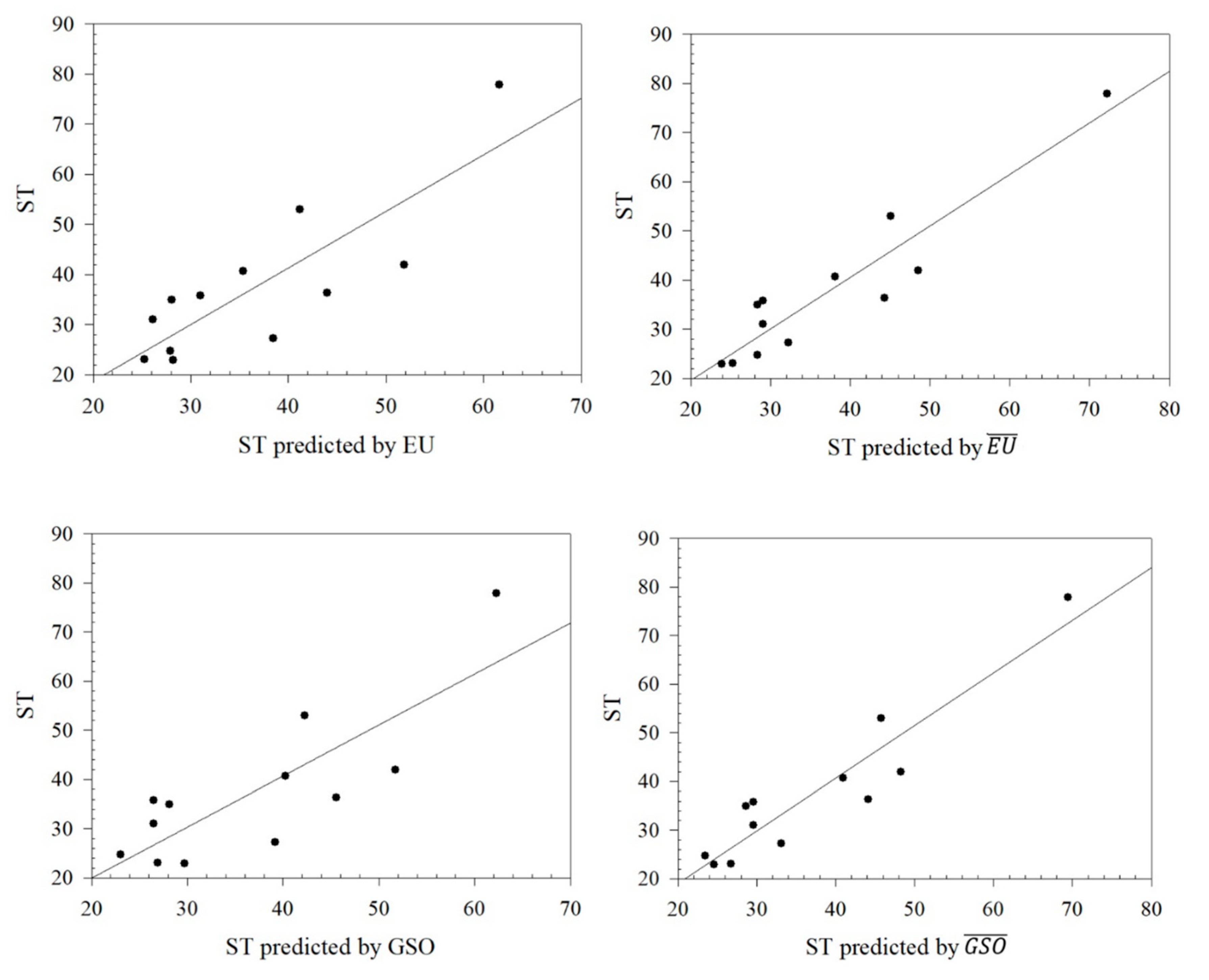
Figure 4.
Graphical relationships between predicted values of ST and its exact values.
5. Results and Discussion
In this study, Gourava Sombor and Euler Sombor coindices are introduced as a new tool in mathematical chemistry and bounds are obtained through union, sum, cartesian product and composition graph operations. Also these indices are studied in some chemical graphs. These results show the important relationship between graph structure and degree concept.
From Table 8, it can be seen that the Euler Sombor and Gourava Sombor topological indices and their coindices are particularly effective in predicting the HBAC, HAC, COMP, and ST properties of butane derivatives. It is observed that the correlation coefficient of the predicted values and the exact values of HBAC is in the range of 0.8419 ≤ R ≤ 0.9277, with the Euler Sombor coindex having the best correlation coefficient of 0.9277. In addition, the correlation coefficient of the predicted and exact values of HAC is in the range of 0.8897 ≤ R ≤ 0.9748, and it gives the best correlation coefficient of 0.9748 with the Euler Sombor coindex, and it is seen that ST is in the range of 0.8137 ≤ R ≤ 0.9344, with the best correlation coefficient being 0.9344 in this index. Finally, the correlation range for Comp is 0.9506 ≤ R ≤ 0.9855, and its best correlation is with the GSO index. It is clear that especially the EU coindex and GSO coindex show very strong correlations with the exact values of the predicted values of the selected physicochemical properties. These strong correlations show that the selected indices are reliable estimators in predicting the physicochemical properties of butane derivatives.
In a related study by Shashidhara et al. [30], the correlation coefficient of predicted and exact values for the studied domination topological indices was in the range of 0.58 ≤ R ≤ 0.88 for HAC, while it was in the range of 0.8897 ≤ R ≤ 0.9748 in our study, For ST, it was in the range of 0.53 ≤ R ≤ 0.83 in [30], while it was in the range of 0.8137 ≤ R ≤ 0.9344 in our study. For Comp, it was in the range of 0.53 ≤ R ≤ 0.90 in [30], while it was in the range of 0.9506 ≤ R ≤ 0.9855 in our study. Thus, in the literature, the highest performance results were obtained with the Gourava Sombor and Euler Sombor indices and especially the coindices in predicting the HAC, COMP and ST physicochemical properties of butane derivatives.
Author Contributions
Conceptualization, S.W. and G.O.-K.; methodology, S.W. and G.O.-K.; validation, S.W.; formal analysis, S.W. and G.O.-K.; investigation, G.O.-K.; writing—review and editing, S.W. and G.O.-K.; visualization, G.O.-K.; su-pervision, S.W.; funding acquisition, S.W. All authors have read and agreed to the published version of the manuscript.
Funding
This research was funded by the Deanship of Scientific Research (DSR) at King Abdulaziz University, Jeddah, under grant no. (GPIP: 580-247-2024). The authors, therefore, acknowledge with thanks DSR for their technical and financial support.
Conflicts of Interest
The authors declare no conflicts of interest.
References
- Bondy, J.A.; Murty, U.S.R. Graph Theory with Applications, 1 Eds., New York: Macmillan Press, (1976).
- Kulli, V.R. College Graph Theory, Gulbarga: Vishwa International Publications, (2012).
- Gutman, I. Geometric approach to degree-based topological indices: Sombor indices. MATCH Commun. Math. Comput. Chem. 2021, 86, 11–16. [Google Scholar]
- Kulli, V.R. Delta Banhatti-Sombor indices of certain networks. Int. J. Math. Comput. Res. 2023, 11, 3875–3881. [Google Scholar] [CrossRef]
- Kulli, V.R. Modified domination Sombor index and its exponential of a graph. Int. J. Math. Comput. Res. 2023, 11, 3639–3644. [Google Scholar] [CrossRef]
- Khalifeh, M.H.; Yousefi-Azari, H.; Ashrafi, A.R. The first and second Zagreb indices of some graph operations. Discrete Appl. Math. 2009, 157, 804–811. [Google Scholar] [CrossRef]
- Furtula, B.; Gutman, I. A forgotten topological index. J. Math. Chem. 2015, 53, 1184–1190. [Google Scholar] [CrossRef]
- Gök, G.K. On the Forgetten Topological Index and Co Index. EJOSAT 2019, 15, 308–314. [Google Scholar] [CrossRef]
- Ashrafi, A.R.; Doslic, T.; Hamzeh, A. The Zagreb coindices of graph operations. Discrete Appl. Math. 2010, 158, 1571–1578. [Google Scholar] [CrossRef]
- Gök, G.K. On The Reformulated Zagreb Coindex. JNT 2019, 28, 28–32. [Google Scholar]
- Das, K.C.; Cevik, A.S.; Shang, Y. On sombor index. Symmetry 2021, 13, 140. [Google Scholar] [CrossRef]
- Du, Z.; You, L.; Liu, H.; Huang, Y. The Sombor index and coindex of two-trees. AIMS Mathematics 2023, 8, 18982–18994. [Google Scholar] [CrossRef]
- Saidi, N.H.A.M.; Husin, M.N.; Ismail, N.B. On the Zagreb Indices of the Line Graphs of Polyphenylene Dendrimers. Journal of Discrete Mathematical Sciences and Cryptography 2020, 23, 1239–1252. [Google Scholar] [CrossRef]
- Redzepovic, I. Chemical Applicability of Sombor Indices. Journal of the Serbian Chemical Society 2021, 86, 445–457. [Google Scholar] [CrossRef]
- Ghalavand, A.; Ashrafi, A.R. On Forgotten Coindex of Chemical Graphs. MATCH Communications in Mathematical and in Computer Chemistry 2020, 83, 221–232. [Google Scholar]
- Du, Z.; You, L.; Liu, H. The Sombor Index and Coindex of Chemical Graphs. Polycyclic Aromatic Compounds 2024, 44, 2942–2965. [Google Scholar] [CrossRef]
- Wazzan, S.; Ahmed, H. Symmetry-adapted domination indices: The enhanced domination sigma index and its applications in QSPR studies of octane and its isomers. Symmetry 2023, 15, 1202. [Google Scholar] [CrossRef]
- Wazzan, S.; Ahmed, H. Advancing computational insights: Domination topological indices of polysaccharides des using special polynomials and QSPR analysis. Contemp. Math. 2024, 5, 26–49. [Google Scholar] [CrossRef]
- Gutman, I.; Furtula, B.; Oz, M.S. Geometric approach to vertex-degree-based topological indices - Elliptic Sombor index, theory and application. Int. J. Quantum Chem 2024, 124, e27346. [Google Scholar] [CrossRef]
- Tang, Z.; Li, Y.; Deng, H. The Euler Sombor index of a graph, Int. J. Quantum Chem. 2024, 124, e27387. [Google Scholar] [CrossRef]
- Kulli, V.R. The Gourava Indices and Coindices of Graphs. Annals of Pure and Applied Mathematics 2014, 1, 33–8. [Google Scholar] [CrossRef]
- Doslic, T. Vertex-weighted wiener polynomials for composite graphs. ARS Math. Contemp. 2008, 1, 66–81. [Google Scholar] [CrossRef]
- Pattabiraman, K.; Vijayaragavan, M. Hyper Zagreb indices and its coindices of graphs. Bull. Inter. Math. Virtual Inst. 2017, 7, 31–41. [Google Scholar]
- De, N.; Nayeem, S.; Pal, A. The F-coindex of some graph operations. SpringerPlus. [CrossRef]
- Alameri, A. New binary operations on graphs. JST 2016, 21, 97–116. [Google Scholar] [CrossRef]
- Dragomir, S.S. A survey on Cauchy-Bunyakovsky-Schwarz type discrete inequalities. J. Inequal. Pure Appl. Math. 2003, 4, 63–202. [Google Scholar]
- Ramirez, R.E.H.; Lijanova, I.V.; Likhanova, N.V.; Xometl, O.O. PAMAM Dendrimers with Porphyrin Core: Synthesis and Metal-Chelating Behavior. Journal of Inclusion Phenomena and Macrocyclic Chemistry 2016, 84, 49–60. [Google Scholar] [CrossRef]
- Manzoor, S.; Siddiqui, M.K.; Ahmad, S. On Computation of Entropy Measures for Phthalocyanines and Porphyrins Dendrimers. International Journal of Quantum Chemistry 2022, 122, e26854. [Google Scholar] [CrossRef]
- PubChem Available from: https://pubchem.ncbi.nlm.nih.
- Shashidhara, A.A.; Ahmed, H.; Nandappa, S.; Cancan, M. Domination version: Sombor index of graphs and its significance in predicting physicochemical properties of butane derivatives. Eurasian Chem. Commun. 2023, 5, 91–102. [Google Scholar] [CrossRef]
Table 1.
Degree Based Topological Indices and Coindices.
| Introduced by | Index Name | Notation | Formula |
| [19,20] | Euler Sombor index | ||
| [21] | Gourava Sombor index | ||
| [22]Doslic, 2008 | First Zagreb coindex | ||
| [22]Doslic, 2008 | Second Zagreb coindex | ||
| [23]Pattabiraman and Vijayaravan, 2017 | First Hyper-Zagreb coindex | ||
| [23]Pattabiraman and Vijayaravan, 2017 | Second Hyper-Zagreb coindex | ||
| [24]De,N.,Abu Nayeem, Sk. Md. and Pal, A. 2016 | Forgetten coindex |
Table 4.
The HBAC values predicted by Gourava and Euer Sombor with coindices.
| Compound | ||||
| 1,4-butanedithiol | 1.335459 | 1.244092 | 1.482178 | 1.508217 |
| 2-butanone | 1.541408 | 1.386579 | 1.139355 | 1.176683 |
| 1,3-butanediol | 1.439583 | 1.377295 | 1.432565 | 1.444889 |
| butane dinitrile | 2.262888 | 1.926617 | 2.122906 | 2.344972 |
| butanediamide | 2.402111 | 2.391729 | 2.660681 | 2.724976 |
| butane-1-sulfoamide | 3.103163 | 3.337642 | 2.933831 | 2.924869 |
| 1-butanethiol | 1.118441 | 1.366671 | 1.431941 | 1.10775 |
| 1,4-diaminobuane | 1.335459 | 1.593424 | 1.482178 | 1.508217 |
| butane-1,4-disulfonic acid | 3.91669 | 4.270912 | 4.990947 | 4.774956 |
| butyraldehyde | 1.361045 | 1.185762 | 1.228135 | 1.317453 |
| 2,3-butanedione | 2.184768 | 2.169334 | 1.69967 | 1.757965 |
| 1-butanesufonylchloride | 2.640528 | 2.628947 | 2.59615 | 2.59299 |
Table 5.
The HAC values predicted by Gourava and Euer Sombor with coindices.
| Compound | ||||
| 1,4-butanedithiol | 5.32036 | 5.112493 | 5.646162 | 5.721763 |
| 2-butanone | 5.776376 | 5.439739 | 4.854167 | 4.978076 |
| 1,3-butanediol | 5.554397 | 5.418869 | 5.536788 | 5.585738 |
| butane dinitrile | 7.198875 | 6.566213 | 6.940683 | 7.328943 |
| butanediamide | 7.449591 | 7.431088 | 7.902143 | 7.973089 |
| butane-1-sulfoamide | 8.627785 | 8.992146 | 8.358541 | 8.296045 |
| 1-butanethiol | 4.805966 | 5.394912 | 5.535402 | 4.812333 |
| 1,4-diaminobuane | 5.32036 | 5.890203 | 5.646162 | 5.721763 |
| butane-1,4-disulfonic acid | 9.859995 | 10.3546 | 11.34251 | 10.92113 |
| butyraldehyde | 5.378571 | 4.973932 | 5.068015 | 5.303816 |
| 2,3-butanedione | 7.055309 | 7.027489 | 6.108283 | 6.235286 |
| 1-butanesufonylchloride | 7.864972 | 7.84426 | 7.79145 | 7.754118 |
Table 6.
The COMP values predicted by Gourava and Euer Sombor with coindices.
| Compound | ||||
| 1,4-butanedithiol | 5.32036 | 5.112493 | 5.646162 | 5.721763 |
| 2-butanone | 5.776376 | 5.439739 | 4.854167 | 4.978076 |
| 1,3-butanediol | 5.554397 | 5.418869 | 5.536788 | 5.585738 |
| butane dinitrile | 7.198875 | 6.566213 | 6.940683 | 7.328943 |
| butanediamide | 7.449591 | 7.431088 | 7.902143 | 7.973089 |
| butane-1-sulfoamide | 8.627785 | 8.992146 | 8.358541 | 8.296045 |
| 1-butanethiol | 4.805966 | 5.394912 | 5.535402 | 4.812333 |
| 1,4-diaminobuane | 5.32036 | 5.890203 | 5.646162 | 5.721763 |
| butane-1,4-disulfonic acid | 9.859995 | 10.3546 | 11.34251 | 10.92113 |
| butyraldehyde | 5.378571 | 4.973932 | 5.068015 | 5.303816 |
| 2,3-butanedione | 7.055309 | 7.027489 | 6.108283 | 6.235286 |
| 1-butanesufonylchloride | 7.864972 | 7.84426 | 7.79145 | 7.754118 |
Table 7.
The ST values predicted by Gourava and Euer Sombor with coindices.
| Compound | ||||
| 1,4-butanedithiol | 5.32036 | 5.112493 | 5.646162 | 5.721763 |
| 2-butanone | 5.776376 | 5.439739 | 4.854167 | 4.978076 |
| 1,3-butanediol | 5.554397 | 5.418869 | 5.536788 | 5.585738 |
| butane dinitrile | 7.198875 | 6.566213 | 6.940683 | 7.328943 |
| butanediamide | 7.449591 | 7.431088 | 7.902143 | 7.973089 |
| butane-1-sulfoamide | 8.627785 | 8.992146 | 8.358541 | 8.296045 |
| 1-butanethiol | 4.805966 | 5.394912 | 5.535402 | 4.812333 |
| 1,4-diaminobuane | 5.32036 | 5.890203 | 5.646162 | 5.721763 |
| butane-1,4-disulfonic acid | 9.859995 | 10.3546 | 11.34251 | 10.92113 |
| butyraldehyde | 5.378571 | 4.973932 | 5.068015 | 5.303816 |
| 2,3-butanedione | 7.055309 | 7.027489 | 6.108283 | 6.235286 |
| 1-butanesufonylchloride | 7.864972 | 7.84426 | 7.79145 | 7.754118 |
Table 8.
The correlation coefficient values of predicted physicochemical properties with its exact values.
Table 8.
The correlation coefficient values of predicted physicochemical properties with its exact values.
| Properties | ||||
| HBAC | 0.8419 | 0.8783 | 0.9277 | 0.9174 |
| HAC | 0.8897 | 0.9221 | 0.9748 | 0.9610 |
| COMP | 0.9855 | 0.9630 | 0.9506 | 0.9619 |
| ST | 0.8137 | 0.8306 | 0.9344 | 0.9332 |
Table 9.
Determination coefficients() for the non-linear QSPR model for the Gourava and Euler Sombor indices(coindices).
Table 9.
Determination coefficients() for the non-linear QSPR model for the Gourava and Euler Sombor indices(coindices).
| Indices | HBAC | HAC | COMP | ST |
|---|---|---|---|---|
| GSO | 0.7464 | 0.7687 | 0.9724 | 0.9840 |
| EU | 0.7840 | 0.8336 | 0.8419 | 0.9751 |
| 0.8322 | 0.9287 | 0.7615 | 0.9867 | |
| 0.8455 | 0.9091 | 0.8366 | 0.9879 |
Disclaimer/Publisher’s Note: The statements, opinions and data contained in all publications are solely those of the individual author(s) and contributor(s) and not of MDPI and/or the editor(s). MDPI and/or the editor(s) disclaim responsibility for any injury to people or property resulting from any ideas, methods, instructions or products referred to in the content. |
© 2025 by the authors. Licensee MDPI, Basel, Switzerland. This article is an open access article distributed under the terms and conditions of the Creative Commons Attribution (CC BY) license (http://creativecommons.org/licenses/by/4.0/).
Copyright: This open access article is published under a Creative Commons CC BY 4.0 license, which permit the free download, distribution, and reuse, provided that the author and preprint are cited in any reuse.


