
Submitted:
27 July 2025
Posted:
28 July 2025
You are already at the latest version
Abstract
To employ some simple physics-inspired density-based information-theoretic approach (ITA) quantities to appreciate the electron correlation energies is an unaccomplished and ongoing task. In this work, we expand the territory of the LR(ITA) (LR means linear regression) protocol to more complex systems, including (i) 24 octane isomers; (ii) polymeric structures, polyyne, polyene, all-trans-polymethineimine, and acene; (iii) molecular clusters, such as metallic Ben and Mgn, covalent Sn, hydrogen-bonded protonated water clusters H+(H2O)n, and dispersion-bound carbon dioxide (CO2)n, and benzene (C6H6)n clusters. With LR(ITA), one can simply predict the post-Hartree‒Fock (such as MP2 and coupled cluster) electron correlation energies at the cost of Hartree‒Fock calculations, even with chemical accuracy. For large molecular clusters, we employ the linear-scaling generalized energy-based fragmentation (GEBF) method to gauge the accuracy of LR(ITA). Employing benzene clusters as an illustration, the LR(ITA) method shows similar accuracy to that of GEBF. Overall, we have verified that ITA quantities can be used to predict the electron correlation energies of various complex systems.
Keywords:
electron correlation energy
; information‐theoretic approach
; generalized energy‐based fragmentation (GEBF)
; molecular clusters
; polymers
1. Introduction
Electron correlation energy lies at the heart of quantum chemistry. [1,2] However, the computational cost of high-level post-Hartree–Fock methods skyrockets with system size. In this context, there is a pressing need for alternative lower-scaling cost-efficient methods across broad classes of systems. In recent years, the information-theoretic approach (ITA) [3,4,5,6] has emerged as a promising framework for understanding and predicting the electron correlation energy from the perspective of information theory. By treating the electron density as a continuous probability distribution, ITA introduces a set of descriptors—such as Shannon entropy [7] and Fisher information [8]—that encode global and local features of the electron density distribution. These quantities are inherently basis-agnostic and physically interpretable, providing a new lens through which quantum chemical problems can be approached.
In continuation with our previous work by employing the simple density-based ITA quantities to appreciate response properties [9,10,11,12,13] (such as molecular polarizability and NMR chemical shielding constant) and energetics of elongated hydrogen chains, [14] in this work, we aim to predict the post-Hartree–Fock (see Figure 1) electron correlation energies of various molecular clusters and linear or quasi-linear organic polymers with increasing cluster size and polymer length. These systems including 24 octane isomers (see Figure 2); [11,15] (ii) polymeric structures (see Figure 3), polyyne, polyene, all-trans-polymethineimine, and acene; [11] (iii) molecular clusters (see Figure 4), such as metallic Benand Mgn, [16,17] covalent Sn, [18,19] hydrogen-bonded protonated water clusters H+(H2O)n, [20] and dispersion-bound carbon dioxide (CO2)n, [21] and benzene clusters (C6H6)n. [22] We construct strong linear relationships between the low-cost Hartree–Fock [23] ITAs and the electron correlation energies from post-Hartree–Fock methods, such as MP2 or RI-MP2, [24,25] CCSD, [26] and CCSD(T). [27] It is noteworthy to mention that MP2 is mainly used here only as a proof-of-concept; Hartree–Fock can be simply replaced with any approximate functionals of density functional theory (DFT) [28,29].
By examining trends across increasing cluster size and polymer length, we assess the transferability, scalability, and physical insights provided by ITA features in capturing electron correlation. Our findings highlight not only the feasibility of ITA-driven correlation energy prediction, but also reveal key descriptors that most strongly govern correlation effects in extended systems. These results suggest that ITA may serve as a promising direction for developing efficient, interpretable, and physically grounded models in quantum machine learning and electronic structure theory.
2. Results
To validate the accuracy of the LR(ITA) method, we choose a total of 24 octane isomers as shown in Figure 2. MP2, CCSD, and CCSD(T) are used to generate the electron correlation energies and ITA quantities are obtained at the Hartree‒Fock level at the same basis set 6-311++G(d,p) level. More details can be found in the Supplementary Information (SI, Table S1). Table 1 shows the linear relationships and RMSDs between the LR(ITA)-predicted and calculated electron correlation energies. For SS, IF, and SGBP, the RMSDs are < 2.0 mH, indicating that LR(ITA) should be accurate enough to predict the electron correlation energies. Because CCSD and CCSD(T) are too computationally-intensive and intractable, only MP2 is used hereafter as proof-of-concept.
In Table 2, Table 3, Table 4 and Table 5, we have collected the linear correlation coefficients (R2 = 1.000) and RMSDs (root mean squared deviations) between the calculated correlation energies at the MP2/6-311++G(d,p) level and those predicted based on the ITA quantities at the HF/6-311++G(d,p) level for polyyne, polyene, all-trans-polymethineimine, and acene, respectively. More details can be found in Tables S2–S5. It is clearly showcased that R2 is close to 1 for most ITA quantities. More strikingly, based on the linear regression (LR) equations of ITA quantities, the predicted electron correlations deviate from the calculated ones only by ~1.5 mH for polyyne, ~3.0 mH for polyene, and < 4.0 mH for all-trans-polymethineimine. For acene, the RMSDs are reasonably satisfactory by ~ 10 ‒ 11 mH. These results collectively reveal that ITA quantities are indeed good descriptors of electron correlations for those linear or quasi-linear polymeric systems with delocalized electronic structures. For more challenging acenes, a single ITA quantity fails to capture sufficient amount of information of more delocalized electronic structures.
Shown in Table 6, Table 7 and Table 8 are the results of the linear correlation coefficients (R2) and RMSDs (root mean squared deviations) between the calculated correlation energies at the MP2/6-311++G(d,p) level and those predicted based on the ITA quantities at the HF/6-311++G(d,p) level for neutral metallic Ben, Mgn, and covalent Sn systems, respectively. More details can be found in Tables S6–S11. One can see that strong correlations exist (R2 > 0.990) between ITA quantities and MP2 correlation energies, indicating that they are extensive in nature. However, the predicted electron correlation energies deviate much from the calculated ones by ~28 ‒ 37 mH for Ben, ~17 ‒ 33 mH for Mgn, and ~26 ‒ 42 mH for Sn, respectively. These results collectively showcase that for 3-dimensional metallic clusters, Ben and Mgn, and covalent Sn, a single ITA quantity fails to quantitively capture enough amount information of electron energies of complex systems.
Shown in Table 9 are the results of the linear correlation coefficients (R2), the corresponding regression coefficients, and RMSDs (root mean squared deviations) between the calculated correlation energies at the MP2/6-311++G(d,p) level and those predicted based on the ITA quantities at the HF/6-311++G(d,p) level for hydrogen-bonded protonated water clusters. One can see that strong correlations exist (R2 = 1.000) between (8 out of 11) ITA quantities and MP2 correlation energies, indicating that they are extensive in nature. The RMSDs range from 2.1 ( and ) to 9.3 () mH, indicating that ITA quantities are good descriptors of the post-Hartree‒Fock electron correlation energies of hydrogen-bonded systems.
Finally, we will switch our gear to two dispersion-bound clusters, (CO2)n and (C6H6)n. Table 10 gives the strong correlations (R2 = 1.000) and RMSDs between the RI-MP2 correlation energies and Hartree‒Fock ITA quantities at the same basis set 6-311++G(d,p) for (CO2)n(n = 4 ‒ 40). More details can be found in Table S12. The RMSDs vary from 6.3 ( and ) to 10.8 () to 14.6 () mH. For (C6H6)n (n = 4 ‒ 14) clusters, we have calculated the linear correlations (R2 = 1.000) and RMSDs between the MP2/6-311++G(d,p) electron correlation energies and HF/6-311++G(d,p) ITA quantities, as collected in Table 11. More details can be found in Tables S13 and S14. The RMSDs range from 2.8 () to 6.9 () to 10.7 () mH. The RMSD results collectively suggest (8 out of 11) ITA quantities are reasonably good descriptors of the post-Hartree‒Fock electron correlation energies of dispersion-bound clusters.
To further verify the accuracy of the LR(ITA) method, we employ some relatively larger (C6H6)n (n = 15 ‒ 30) clusters to this end. Plus, conventional MP2/6-311++G(d,p) calculations are too computationally-intensive, we employ GEBF [30,31,32,33] to obtain the MP2-level electron correlation energies as reference. Finally, as the linear regression based on the ITA quantity has the least RMSD value, we choose LR(G3) to make predictions of electron correlation energies of benzene clusters. More details can be found in Tables 15 and 16. Figure 5 shows a comparison of the LR(G3)-predicted and GEBF-calculated MP2 electron correlation energies for benzene clusters. The RMSD is 8.6 mH, indicative that the LR(ITA) method has a comparable performance to the linear-scaling GEBF method. In addition, we have found that when subsystem wavefunctions (thus electron density and ITA quantities) are used to obtain the subsystem electron correlation energies, the final total electron correlation energies deviate from GEBF by 40.0 mH in terms of RMSD as shown in Table S16. One possible for this observation may come from the error accumulation, rather than error cancellation.
3. Discussion
To accurately and efficiently predict the post-Hartree‒Fock electron correlation energy at a relatively low cost is a hot area in the community of quantum chemistry. Starting from Hartree‒Fock molecular orbitals, there exist two typical methods. One is to calculate the local correlation energy, whose early development is due to Pulay and Sæbø; [34,35,36] the other is to predict the correlation energy with the aid of deep learning (DL). [37,38,39,40,41,42,43,44,45,46] Our proposed LR(ITA) method is a special favor of DL. Suffice to note that an inherent drawback of local correlation methods is to perform orbital localization. This problem is also encountered by the DL-driven method. For our LR(ITA) method, only the molecular orbitals (thus electron density) are required without any manipulation. Very recently, we have showcased the good accuracy of LR(ITA) and its variant DL(ITA). With LR(ITA), one can even predict the FCI-level electron correlation with the DMRG (density matrix renormalization group) algorithm as a solver for elongated hydrogen chain, [14] and the RMSD is only a few mH. Moreover, with DL(ITA) where a total 11 ITA quantities are used as input, [13] we have predicted the DLPNO-MP2 electron correlation energy for a database of > 90 K real organic molecules and the RMSD is about 6.8 mH. In addition, LR(ITA) is not limited to any post-Hartree‒Fock electronic structure methods; MP2 is used here as a proof-of-concept. Thus, we have showcased that LR(ITA) is designed with architectural and conceptual simplicity and is numerically shown to be a good protocol to predict the electron correlation energies of various systems.
Admittedly, using LR(ITA) to accurately and efficiently predict the electron correlation energy is still in its infancy. In the near future, we will implement a new concept of “ITL-DL Loop”. The physics behind is simple: low-tier (such as semiempirical PM7 or even promolecular) electron densities are used as input for ITA quantities, and DL is introduced to obtain high-tier (such as DFT) electron densities. Based on the newly generated electron densities, ITA quantities are obtained and used as input for another either classical or quantum DL model to predict the electron correlation energies of electrons of physicochemical properties of molecules. Work along this line is in progress and the results will be presented elsewhere.
4. Materials and Methods
4.1. Information-Theoretic Approach Quantities
Shannon entropy [7] and Fisher information [8] are two foundational quantities in information theory. They are defined as Equations (1) and (2), respectively.
where is the electron density and is the density gradient. Physically, characterizes the spatial delocalization of the electron density, while reflects its sharpness or localization. Of note, and are not mutually exclusive and but always intercorrelated.
Beyond the total electron density, additional quantities such as kinetic-energy density can be incorporated into the formulation of information-theoretic approaches (ITA). Utilizing both electron density and kinetic-energy density, Ghosh, Berkowitz, and Parr introduced an entropy functional known as (), [47]
where t(r; ρ) and tTF(r; ρ) represent the non-interacting and Thomas–Fermi (TF) kinetic energy density, respectively. The constants are defined as follows: k is the Boltzmann constant, c = (5/3) +ln(4πcK/3), and cK = (3/10)(3π2)2/3]. The non-interacting kinetic energy density integrates to give the total kinetic energy ,
It can be computed from the canonical orbital densities as,
while the Thomas–Fermi expression is given by,
It is important to note that kinetic-energy density may take different forms depending on context. [48,49,50,51,52,53,54,55] Nonetheless, SGBP satisfies the maximum-entropy principle from a rigorous mathematical viewpoint. [47]
Expanding further, several ITA descriptors have been proposed to characterize chemical reactivity. Within the framework of conceptual density functional theory (CDFT), [56,57,58,59,60] one such example is relative Rényi entropy [60] of order n
Another related measure is information gain () [61], also called Kullback−Leibler divergence or relative Shannon entropy,
In both expressions (7) and (8), is a reference-state density, and both and are normalized.
More recently, [62] one of the present authors introduced three ITA descriptors G1, G2, and G3, applicable at both atomic and molecular levels:
Finally, to partition electron density into atomic contributions within a molecule, the Hirshfeld stockholder approach [63,64] is frequently adopted. It is defined as:
Here, is the atomic (Hirshfeld) density, is the weight or “sharing” function, represents the reference (typically spherically averaged) atomic density centered at . The denominator is known as the promolecular density. The stockholder method naturally aligns with ITA due to its information-theoretic foundation. Alternative partitioning schemes include Becke’s fuzzy atom method [65] and Bader’s atoms-in-molecules (AIM) approach based on zero-flux surfaces [66]. A summary of our recent work in this direction is available in Refs [67,68,69].
4.2. An Outline of GEBF
In the generalized energy-based fragmentation (GEBF) method, [30,31,32,33] the total energy of a large system—such as a macromolecule or molecular aggregate—is expressed as a linear combination of the energies of smaller embedded subsystems, as given in Equation (13):
Here, Em and Cm stand for the total energy and the coefficient of the mth subsystem, respectively. QA, is the atomic charge on atom A. RAB is the interatomic distance between atoms A and B.
The general procedure for performing GEBF calculations involves several steps. Employing a molecular cluster of benzene (C6H6) as illustrated in Figure 4f, each benzene molecule is treated as a fragment. Primitive subsystems are then constructed centered at each fragment, defined by a distance threshold (ζ). These primitive subsystems are assigned coefficients Cm = +1. Due to the spatial overlap among primitive subsystems, smaller derivative subsystems are generated. The coefficients of these derivative subsystems are determined automatically using the principle of inclusion and exclusion, ensuring proper energy accounting. Another parameter, γmax, representing the maximum number of fragments allowed in a subsystem, is introduced to control subsystem size.
All quantum chemical calculations for the subsystems are carried out using the GEBF method as implemented in the LSQC (low scaling quantum chemistry) package. [70] In this work, the two key GEBF parameters, (ζ, γmax) are set to be (4.0, 6).
4.3. Computational Details
A total of 24 of octane isomers, metallic clusters Ben (n =3 to 25), Mgn (n = 3 to 20 and 28), (CO2)n (n = 4 to 40), organic clusters of (C6H6)n (n = 4 to 30), covalent Sn (n =2 to 18); polymeric structures (see Figure 2) of polyyne, polyene, all-trans-polymethineimine, and acene, were taken from our previous publication. For the protonated clusters [(H2O)n(H3O)]+ , they were taken from Ref 20. For cluster sizes n = 10, 11, 12, 13, 14, 15, 16, 17, 18, 19, and 20, there are 74, 79, 113, 119, 108, 140, 121, 138, 114, 125, and 143 structures, respectively.
Molecular wavefunctions for all the systems were obtained at the HF/6-311++G(d,p) level. The Multiwfn 3.8 [71,72] program was utilized to calculate all ITA quantities by using the Gaussian 16 checkpoint or wavefunction file as the input. The stockholder Hirshfeld partition scheme of atoms in molecules was employed when atomic contributions were concerned. The reference-state density was the neutral atom calculated at the restricted open-shell ROHF/6-311++G(d,p) level. CCSD and CCSD(T) calculations for octane isomers were performed with the Gaussian 16 [73] package. For RI-MP2 calculations, Hartree‒Fock (HF) orbitals from the Gaussian 16 calculations were then transformed into the ORCA [74] format by using the MOKIT [75] program. The frozen core formalism [76] was used throughout this work, unless otherwise stated.
5. Conclusions
To summarize, in this work, we have applied the information-theoretic approach (ITA) quantities to appreciate the post-Hartree‒Fock (such as MP2 or RI-MP2) correlation energies for various molecular clusters and polymeric systems with both localized and delocalized electronic structures. We have found that for linear or quasi-linear polymeric systems, such as polyyne and polyene, the predicted results based on the Hartree‒Fock ITA quantities, are in excellent agreement with the calculated MP2 correlation energies. For other systems, such as hydrogen-bonded protonated water clusters and dispersion-bound carbon dioxide and benzene clusters, satisfactory results can be obtained with the LR(ITA) protocol. For metallic Ben and Mgn, as well as covalent Sn, one can still obtain reasonable results. In addition, for relatively larger benzene clusters, we compare the LR(ITA) results with those from the GEBF method and similar accuracy is observed. Our results collectively showcase that LR(ITA) is a promising method as a cost-efficient tool in predict the electron correlation energy.
Supplementary Materials
The following supporting information can be downloaded at the website of this paper posted on Preprints.org, Hartree‒Fock ITA quantities, the electron correlation energies and the total energies, and linear regression coefficients and correlation coefficients.
Author Contributions
Conceptualization, S.L., P.W.A. and D.Z.; data curation, X.H. and D.Z.; formal analysis, X.H. and D.Z.; funding acquisition, P.W.A. and D.Z.; project administration, S.L. P.W.A. and D.Z.; supervision, S.L., P.W.A. and D.Z.; writing—original draft, D.Z.; writing—review and editing, S.L., P.W.A. and D.Z. All authors have read and agreed to the published version of the manuscript. All authors have read and agreed to the published version of the manuscript.
Funding
This work is supported by the National Natural Science Foundation of China (grant no. 22203071 and 22361051), the High-Level Talent Special Support Plan, the China Scholarship Council, NSERC, Canada Research Chairs, and the Digital Research Alliance of Canada.
Institutional Review Board Statement
Not applicable.
Informed Consent Statement
Not applicable.
Data Availability Statement
Data are contained within the article.
Acknowledgments
Part of the computations were performed on the high-performance computers of the Advanced Computing Center of Yunnan University.
Conflicts of Interest
The authors declare no conflicts of interest.
References
- Szabo, A.; Ostlund, N.S. Modern Quantum Chemistry: Introduction to Advanced Electronic Structure Theory; Dover Publications, 1996. [Google Scholar]
- Tew, D.P.; Klopper, W.; Helgaker, T. Electron correlation: The many-body problem at the heart of chemistry. J. Comput. Chem. 2007, 28, 1307–1320. [Google Scholar] [CrossRef]
- Nalewajski, R.F.; Parr, R.G. Information theory, atoms in molecules, and molecular similarity. Proc. Natl. Acad. Sci. U.S.A. 2000, 97, 8879–8882. [Google Scholar] [CrossRef]
- Ayers, P.W. Information Theory, the Shape Function, and the Hirshfeld Atom. Theor. Chem. Acc. 2006, 115, 370–378. [Google Scholar] [CrossRef]
- Zhao, Y.; Zhao, D.; Rong, C.; Liu, S.; Ayers, P.W. Information Theory Meets Quantum Chemistry: A Review and Perspective. Entropy 2025, 27, 644. [Google Scholar] [CrossRef] [PubMed]
- Zhao, Y.; Zhao, D.; Rong, C.; Liu, S.; Ayers, P.W. Extending the information-theoretic approach from the (one) electron density to the pair density. J. Chem. Phys. 2025, 162, 244108. [Google Scholar] [CrossRef]
- Shannon, C.E. A mathematical theory of communication. Bell Syst. Tech. J. 1948, 27, 379–423. [Google Scholar] [CrossRef]
- Fisher, R.A. Theory of statistical estimation. Math. Proc. Camb. Philos. Soc. 1925, 22, 700–725. [Google Scholar] [CrossRef]
- Zhao, D.; Liu, S.; Chen, D. A Density Functional Theory and Information-Theoretic Approach Study of Interaction Energy and Polarizability for Base Pairs and Peptides. Pharmaceuticals 2022, 15, 938. [Google Scholar] [CrossRef] [PubMed]
- Zhao, D.; He, X.; Ayers, P.W.; Liu, S. Excited-State Polarizabilities: A Combined Density Functional Theory and Information-Theoretic Approach Study. Molecules 2023, 28, 2576. [Google Scholar] [CrossRef]
- Zhao, D.; Zhao, Y.; He, X.; Ayers, P.W.; Liu, S. Efficient and accurate density-based prediction of macromolecular polarizabilities. Phys. Chem. Chem. Phys. 2023, 25, 2131–2141. [Google Scholar] [CrossRef]
- Zhao, D.; Zhao, Y.; Xu, E.; Liu, W.; Ayers, P.W.; Liu, S.; Chen, D. Fragment-Based Deep Learning for Simultaneous Prediction of Polarizabilities and NMR Shieldings of Macromolecules and Their Aggregates. J. Chem. Theory Comput. 2024, 20, 2655–2665. [Google Scholar] [CrossRef]
- Yuan, Y.; Zhao, Y.; Lu, L.; Wang, J.; Chen, J.; Ayers, P.W.; Liu, S.; Zhao, D. Multi-property Deep Learning of the Correlation Energy of Electrons and the Physicochemical Properties of Molecules. J. Chem. Theory Comput. 2025, 21, 5997–6006. [Google Scholar] [CrossRef]
- Zhao, Y.; Richer, M.; Ayers, P.W.; Liu, S.; Zhao, D. Can the FCI Energies/Properties be Predicted with HF/DFT Densities? J. Chem. Sci. 2025. submitted. [Google Scholar]
- Luo, C.; He, X.; Zhong, A.; Liu, S.; Zhao, D. What dictates alkane isomerization? A combined density functional theory and information-theoretic approach study. Theor. Chem. Acc. 2023, 142, 78. [Google Scholar] [CrossRef]
- Abyaz, B.; Mahdavifar, Z.; Schreckenbach, G.; Gao, Y. Prediction of beryllium clusters (Ben; n = 3 – 25) from first principles. Phys. Chem. Chem. Phys. 2021, 23, 19716–19728. [Google Scholar] [CrossRef] [PubMed]
- Duanmu, K.; Friedrich, J.; Truhlar, D.G. Thermodynamics of Metal Nanoparticles: Energies and Enthalpies of Formation of Magnesium Clusters and Nanoparticles as Large as 1.3 nm. J. Phys. Chem. C 2016, 120, 26110–26118. [Google Scholar] [CrossRef]
- Raghavachari, K. Structures and stabilities of sulfur clusters. J. Chem. Phys. 1990, 93, 5862–5874. [Google Scholar] [CrossRef]
- Jones, R.O.; Ballone, P. Density functional and Monte Carlo studies of sulfur. I. Structure and bonding in Sn rings and chains (n = 2–18). J. Chem. Phys. 2003, 118, 9257–9265. [Google Scholar] [CrossRef]
- Ng, W.-P.; Zhang, Z.; Yang, J. Accurate Neural Network Fine-Tuning Approach for Transferable Ab Initio Energy Prediction across Varying Molecular and Crystalline Scales. J. Chem. Theory Comput 2025, 21, 1602–1614. [Google Scholar] [CrossRef]
- Takeuchi, H. Geometry Optimization of Carbon Dioxide Clusters (CO2)n for 4 ≤ n ≤ 40. J. Phys. Chem. A 2008, 112, 7492–7497. [Google Scholar] [CrossRef]
- Takeuchi, H. Structural Features of Small Benzene Clusters (C6H6)n (n ≤ 30) As Investigated with the All-Atom OPLS Potential. J. Phys. Chem. A 2012, 116, 10172–10181. [Google Scholar] [CrossRef]
- Roothaan, C.C.J. New Developments in Molecular Orbital Theory. Rev. Mod. Phys. 1951, 23, 69–89. [Google Scholar] [CrossRef]
- Møller, C.; Plesset, M.S. Note on an Approximation Treatment for Many-Electron Systems. Phys. Rev. 1934, 46, 618–622. [Google Scholar] [CrossRef]
- Weigend, F.; Ahlrichs, R. Efficient use of the correlation consistent basis sets in resolution of the identity MP2 calculations. Chem. Phys. Lett. 1997, 294, 143–152, (b) Weigend, F. RI-MP2: optimized auxiliary basis sets and demonstration of efficiency. Phys. Chem. Chem. Phys. 2002, 4, 4285’4291. [Google Scholar] [CrossRef]
- Bartlett, R.J.; Watts, J.D. The coupled-cluster single and double excitation model for the ground-state correlation energy. Chem. Phys. Lett. 1989, 155, 133–140, (b) Čížek, J.; Paldus, J. Coupled-cluster method with singles and doubles for closed‐shell systems. Int. J. Quantum Chem. 1971, 5, 359–379.. [Google Scholar] [CrossRef]
- Purvis, G.D.; Bartlett, R.J. A full coupled-cluster singles and doubles model: The inclusion of disconnected triples. J. Chem. Phys. 1982, 76, 1910–1918. [Google Scholar] [CrossRef]
- Parr, R.G.; Yang, W. Density Functional Theory of Atoms and Molecules; Oxford University Press: Oxford, UK, 1989. [Google Scholar]
- Teale, A.M.; Helgaker, T.; Savin, A.; Adamo, C.; Aradi, B.; Arbuznikov, A.V.; Ayers, P.W.; Baerends, E.J.; Barone, V.; Calaminici, P.; Cancès, E.; Carter, E.A.; Chattaraj, P.K.; Chermette, H.; Ciofini, I.; Crawford, T.D.; De Proft, F.; Dobson, J.F.; Draxl, C.; Frauenheim, T.; Fromager, E.; Fuentealba, P.; Gagliardi, L.; Galli, G.; Gao, J.; Geerlings, P.; Gidopoulos, N.; Gill, P.M.W.; Gori-Giorgi, P.; Görling, A.; Gould, T.; Grimme, S.; Gritsenko, O.; Jensen, H.J.A.; Johnson, E.R.; Jones, R.O.; Kaupp, M.; Köster, A.M.; Kronik, L.; Krylov, A.I.; Kvaal, S.; Laestadius, A.; Levy, M.; Lewin, M.; Liu, S.; Loos, P.-F.; Maitra, N.T.; Neese, F.; Perdew, J.P.; Pernal, K.; Pernot, P.; Piecuch, P.; Rebolini, E.; Reining, L.; Romaniello, P.; Ruzsinszky, A.; Salahub, D.R.; Scheffler, M.; Schwerdtfeger, P.; Staroverov, V.N.; Sun, J.; Tellgren, E.; Tozer, D.J.; Trickey, S.B.; Ullrich, C.A.; Vela, A.; Vignale, G.; Wesolowski, T.A.; Xu, X.; Yang, W. DFT exchange: sharing perspectives on the workhorse of quantum chemistry and materials science. Phys. Chem. Chem. Phys. 2022, 24, 28700–28781. [Google Scholar] [CrossRef]
- Li, S.; Li, W.; Fang, T. An Efficient Fragment-Based Approach for Predicting the Ground-State Energies and Structures of Large Molecules. J. Am. Chem. Soc. 2005, 127, 7215–7226. [Google Scholar] [CrossRef]
- Li, W.; Li, S.; Jiang, Y. Generalized Energy-Based Fragmentation Approach for Computing the Ground-State Energies and Properties of Large Molecules. J. Phys. Chem. A 2007, 111, 2193–2199. [Google Scholar] [CrossRef]
- Li, S.; Li, W.; Ma, J. Generalized Energy-Based Fragmentation Approach and Its Applications to Macromolecules and Molecular Aggregates. Acc. Chem. Res. 2014, 47, 2712–2720. [Google Scholar] [CrossRef]
- Li, W.; Dong, H.; Ma, J.; Li, S. Structures and Spectroscopic Properties of Large Molecules and Condensed-Phase Systems Predicted by Generalized Energy-Based Fragmentation Approach. Acc. Chem. Res. 2021, 54, 169–181. [Google Scholar] [CrossRef] [PubMed]
- Pulay, P. Localizability of dynamic electron correlation. Chem. Phys. Lett. 1983, 100, 151–154. [Google Scholar] [CrossRef]
- Sæbø, S.; Pulay, P. Local configuration interaction: An efficient approach for larger molecules. Chem. Phys. Lett. 1985, 113, 13–18. [Google Scholar] [CrossRef]
- Sæbø, S.; Pulay, P. Local Treatment of Electron Correlation. Annu. Rev. Phys. Chem. 1993, 44, 213–236. [Google Scholar] [CrossRef]
- Welborn, M.; Cheng, L.; Miller, T.F. III Transferability in Machine Learning for Electronic Structure via the Molecular Orbital Basis. J. Chem. Theory Comput. 2018, 14, 4772–4779. [Google Scholar] [CrossRef]
- Cheng, L.; Welborn, M.; Christensen, A.S.; Miller, T.F. III A universal density matrix functional from molecular orbital-based machine learning: Transferability across organic molecules. J. Chem. Phys. 2019, 150, 131103. [Google Scholar] [CrossRef]
- Cheng, L.; Kovachki, N.B.; Welborn, M.; Miller, T.F. III Regression Clustering for Improved Accuracy and Training Costs with Molecular-Orbital-Based Machine Learning. J. Chem. Theory Comput. 2019, 15, 6668–6677. [Google Scholar] [CrossRef] [PubMed]
- Imamura, Y.; Takahashi, A.; Nakai, H. Grid-based energy density analysis: Implementation and assessment. J. Chem. Phys. 2007, 126, 034103. [Google Scholar] [CrossRef]
- Nudejima, T.; Ikabata, Y.; Seino, J.; Yoshikawa, T.; Nakai, H. Machine-learned electron correlation model based on correlation energy density at complete basis set limit. J. Chem. Phys. 2019, 151, 024104. [Google Scholar] [CrossRef] [PubMed]
- Han, R.; Luber, S. Fast Estimation of Møller−Plesset Correlation Energies Based on Atomic Contributions. J. Phys. Chem. Lett. 2021, 12, 5324–5331. [Google Scholar] [CrossRef] [PubMed]
- Han, R.; Rodríguez-Mayorga, M.; Luber, S. A Machine Learning Approach for MP2 Correlation Energies and Its Application to Organic Compounds. J. Chem. Theory Comput. 2021, 17, 777–790. [Google Scholar] [CrossRef] [PubMed]
- Ng, W.-P.; Liang, Q.; Yang, J. Low-Data Deep Quantum Chemical Learning for Accurate MP2 and Coupled-Cluster Correlations. J. Chem. Theory Comput. 2023, 19, 5439–5449. [Google Scholar] [CrossRef]
- Townsend, J.; Vogiatzis, K.D. Transferable MP2-Based Machine Learning for Accurate Coupled-Cluster Energies. J. Chem. Theory Comput. 2020, 16, 7453–7461. [Google Scholar] [CrossRef]
- McGibbon, R.T.; Taube, A.G.; Donchev, A.G.; Siva, K.; Hernández, F.; Hargus, C.; Law, K.-H.; Klepeis, J.L.; Shaw, D.E. Improving the accuracy of Møller-Plesset perturbation theory with neural networks. J. Chem. Phys. 2017, 147, 161725. [Google Scholar] [CrossRef]
- Ghosh, S.K.; Berkowitz, M.; Parr, R.G. Transcription of ground-state density-functional theory into a local thermodynamics. Proc. Natl. Acad. Sci. U.S.A. 1984, 81, 8028–8031. [Google Scholar] [CrossRef]
- Bader, R.F.W.; Preston, H.J.T. The kinetic energy of molecular charge distributions and molecular stability. Int. J. Quantum Chem. 1969, 3, 327–347. [Google Scholar] [CrossRef]
- Tal, Y.; Bader, R.F.W. Studies of the energy density functional approach. I. Kinetic energy. Int. J. Quantum Chem. 1978, 14, 153–168. [Google Scholar] [CrossRef]
- Cohen, L. Local kinetic energy in quantum mechanics. J. Chem. Phys. 1979, 70, 788–789. [Google Scholar] [CrossRef]
- Cohen, L. Representable local kinetic energy. J. Chem. Phys. 1984, 80, 4277–4279. [Google Scholar] [CrossRef]
- Yang, Z.; Liu, S.; Wang, Y.A. Uniqueness and Asymptotic Behavior of the Local Kinetic Energy. Chem. Phys. Lett. 1996, 258, 30–36. [Google Scholar] [CrossRef]
- Ayers, P.W.; Parr, R.G.; Nagy, Á. Local kinetic energy and local temperature in the density-functional theory of electronic structure. Int. J. Quantum Chem. 2002, 90, 309–326. [Google Scholar] [CrossRef]
- Anderson, J.S.M.; Ayers, P.W.; Hernandez, J.I.R. How Ambiguous Is the Local Kinetic Energy? J. Phys. Chem. A 2010, 114, 8884–8895. [Google Scholar] [CrossRef]
- Berkowitz, M. Exponential approximation for the density matrix and the Wigner distribution. Chem. Phys. Lett. 1986, 129, 486–488. [Google Scholar] [CrossRef]
- Geerlings, P.; De Proft, F.; Langenaeker, W. Conceptual Density Functional Theory. Chem. Rev. 2003, 103, 1793–1874. [Google Scholar] [CrossRef]
- Johnson, P.A.; Bartolotti, L.J.; Ayers, P.W.; Fievez, T.; Geerlings, P. Charge density and chemical reactivity: A unified view from conceptual DFT. In Modern Charge Density Analysis; Gatti, C., Macchi, P., Eds.; Springer: New York, 2012. [Google Scholar]
- Liu, S. Conceptual Density Functional Theory and Some Recent Developments. Acta Phys.-Chim. Sin. 2009, 25, 590–600. [Google Scholar]
- Geerlings, P.; Chamorro, E.; Chattaraj, P.K.; De Proft, F.; Gázquez, J.L.; Liu, S.; Morell, C.; Toro-Labbé, A.; Vela, A.; Ayers, P.W. Conceptual density functional theory: status, prospects, issues. Theor. Chem. Acc. 2020, 139, 36. [Google Scholar] [CrossRef]
- Liu, S.; Rong, C.; Wu, Z.; Lu, T. Rényi entropy, Tsallis entropy and Onicescu information energy in density functional reactivity theory. Acta Phys.-Chim. Sin. 2015, 31, 2057–2063. [Google Scholar] [CrossRef]
- Kullback, S. Information Theory and Statistics; Dover Publications: Mineola, NY, 1997. [Google Scholar]
- Liu, S. Identity for Kullback-Leibler divergence in density functional reactivity theory. J. Chem. Phys. 2019, 151, 141103. [Google Scholar] [CrossRef] [PubMed]
- Hirshfeld, F.L. Bonded-atom fragments for describing molecular charge densities. Theor. Chim. Acta 1977, 44, 129–138. [Google Scholar] [CrossRef]
- Heidar-Zadeh, F.; Ayers, P.W.; Verstraelen, T.; Vinogradov, I.; Vohringer-Martinez, E.; Bultinck, P. Information-Theoretic Ap-proaches to Atoms-in-Molecules: Hirshfeld Family of Partitioning Schemes. J. Phys. Chem. A 2018, 122, 4219–4245. [Google Scholar] [CrossRef]
- Becke, A.D. A multicenter numerical integration scheme for polyatomic molecules. J. Chem. Phys. 1988, 88, 2547–2553. [Google Scholar] [CrossRef]
- Bader, R.F.W. Atoms in Molecules: A Quantum Theory; Clarendon Press, 1990. [Google Scholar]
- Rong, C.; Wang, B.; Zhao, D.; Liu, S. Information-Theoretic approach in density functional theory and its recent applications to chemical problems. Wiley Interdiscip. Rev.: Comput. Mol. Sci. 2020, 10, e1461. [Google Scholar] [CrossRef]
- Rong, C.; Zhao, D.; He, X.; Liu, S. Development and Applications of the Density-Based Theory of Chemical Reactivity. J. Phys. Chem. Lett. 2022, 13, 11191–11200. [Google Scholar] [CrossRef] [PubMed]
- He, X.; Li, M.; Rong, C.; Zhao, D.; Liu, W.; Ayers, P.W.; Liu, S. Some Recent Advances in Density-Based Reactivity Theory. J. Phys. Chem. A 2024, 128, 1183–1196. [Google Scholar] [CrossRef]
- Li, W.; Chen, C.; Zhao, D.; Li, S. LSQC: Low scaling quantum chemistry program. Int. J. Quantum Chem. 2015, 115, 641–646. [Google Scholar] [CrossRef]
- Lu, T.; Chen, F. Multiwfn: A multifunctional wavefunction analyzer. J. Comput. Chem. 2012, 33, 580–592. [Google Scholar] [CrossRef]
- Lu, T. A comprehensive electron wavefunction analysis toolbox for chemists, Multiwfn. J. Chem. Phys. 2024, 161, 082503. [Google Scholar] [CrossRef]
- Frisch, M.J.; Trucks, G.W.; Schlegel, H.B.; Scuseria, G.E.; Robb, M.A.; Cheeseman, J.R.; Scalmani, G.; Barone, V.; Petersson, G.A.; Nakatsuji, H.; Li, X.; Caricato, M.; Marenich, A.V.; Bloino, J.; Janesko, B.G.; Gomperts, R.; Mennucci, B.; Hratchian, H.P.; Ortiz, J.V.; Izmaylov, A.F.; Sonnenberg, J.L.; Williams-Young, D.; Ding, F.; Lipparini, F.; Egidi, F.; Goings, J.; Peng, B.; Petrone, A.; Henderson, T.; Ranasinghe, D.; Zakrzewski, V.G.; Gao, J.; Rega, N.; Zheng, G.; Liang, W.; Hada, M.; Ehara, M.; Toyota, K.; Fukuda, R.; Hasegawa, J.; Ishida, M.; Nakajima, T.; Honda, Y.; Kitao, O.; Nakai, H.; Vreven, T.; Throssell, K.; Montgomery, J.A., Jr.; Peralta, J.E.; Ogliaro, F.; Bearpark, M.J.; Heyd, J.J.; Brothers, E.N.; Kudin, K.N.; Staroverov, V.N.; Keith, T.A.; Kobayashi, R.; Normand, J.; Raghavachari, K.; Rendell, A.P.; Burant, J.C.; Iyengar, S.S.; Tomasi, J.; Cossi, M.; Millam, J.M.; Klene, M.; Adamo, C.; Cammi, R.; Ochterski, J.W.; Martin, R.L.; Morokuma, K.; Farkas, O.; Foresman, J.B.; Fox, D.J. Gaussian 16 Rev. C.01; Wallingford, CT, 2016.
- Zou, J. Molecular Orbital Kit (MOKIT). Available online: https://gitlab.com/jxzou/mokit (accessed on 20 May 2025).
- Neese, F. Software update: The ORCA program system—Version 5.0. Wiley Interdiscip. Rev.: Comput. Mol. Sci. 2022, 12, e1606. [Google Scholar] [CrossRef]
- Pulay, P.; Saebø, S. Orbital-invariant formulation and second-order gradient evaluation in Møller–Plesset perturbation theory. Theor. Chim. Acta 1986, 69, 357–368, (b) Hampel, C.; Peterson, K.; Werner, H. A comparison of the efficiency and accuracy of different electron correlation methods for large molecules: Quasi-Newton, MP2, CCSD, and CCSD(T). Chem. Phys. Lett. 1992, 190, 1–12.. [Google Scholar] [CrossRef]
Figure 1.
Comparison of (a) conventional MP2 method (with Hartree‒Fock orbitals as input) and (b) linear regression LR(ITA) models used in this work, where the density-based information-theoretic approach (ITA) quantities are used as input. Here MP2 is used only as a proof-of-concept.
Figure 1.
Comparison of (a) conventional MP2 method (with Hartree‒Fock orbitals as input) and (b) linear regression LR(ITA) models used in this work, where the density-based information-theoretic approach (ITA) quantities are used as input. Here MP2 is used only as a proof-of-concept.
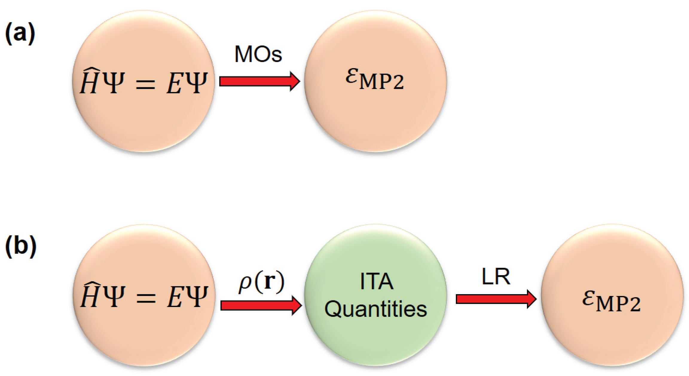
Figure 2.
Shown here are a total of 24 isomers of both branched and linear octane studied in this work.
Figure 2.
Shown here are a total of 24 isomers of both branched and linear octane studied in this work.
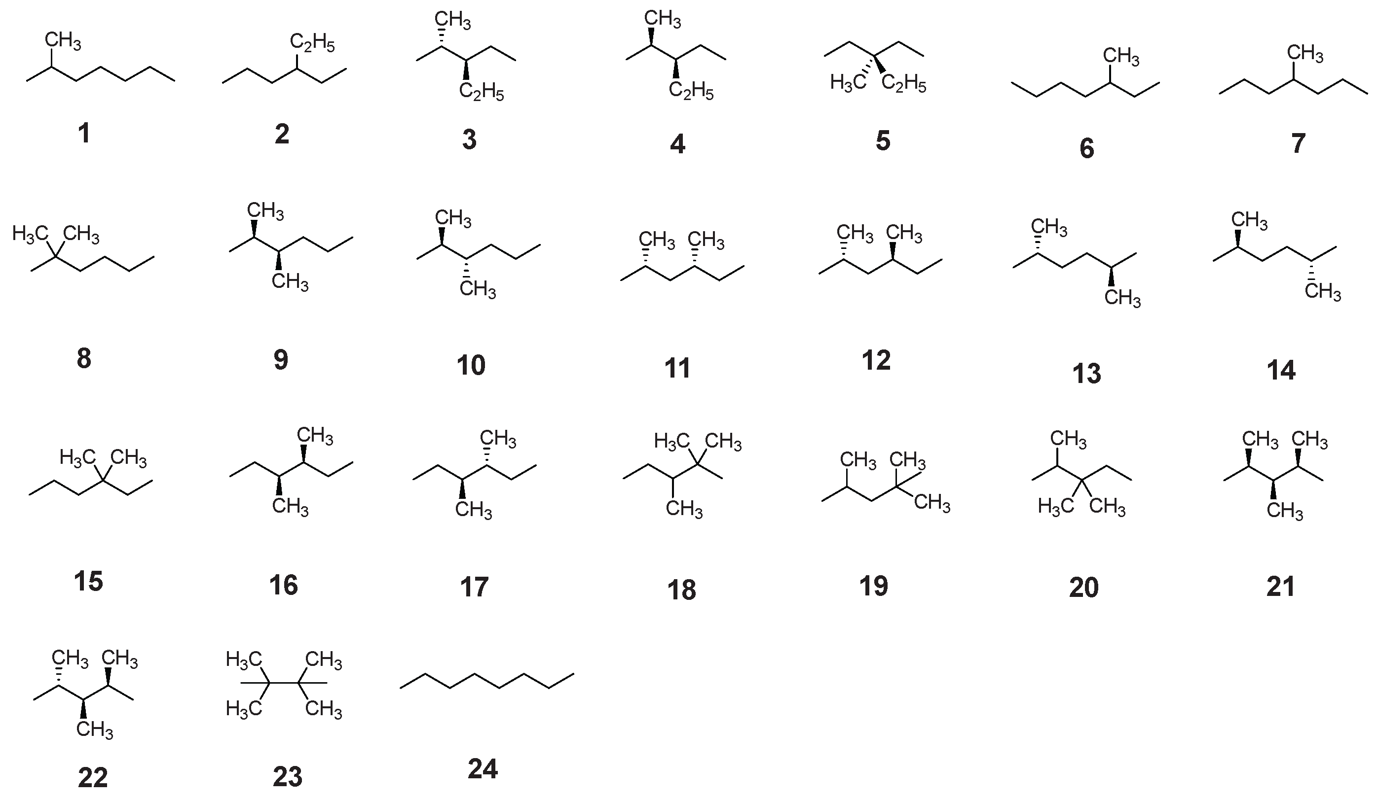
Figure 3.
Some representative polymeric structures used in this work, including (a) polyyne, (b) polyene, (c) all-trans-polymethineimine, and (d) acene.
Figure 3.
Some representative polymeric structures used in this work, including (a) polyyne, (b) polyene, (c) all-trans-polymethineimine, and (d) acene.
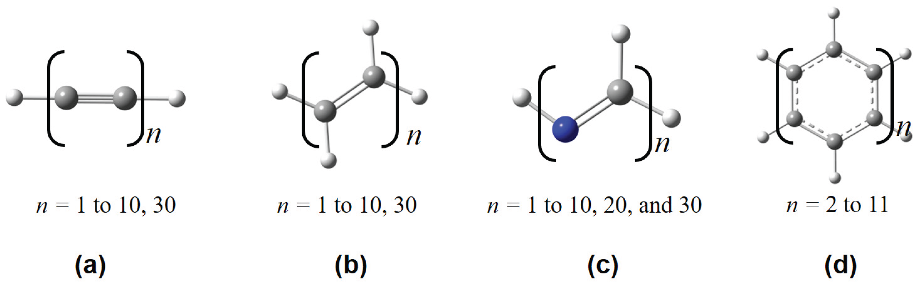
Figure 4.
Some representative molecular structures used in this work, including (a) Ben, (b) Mgn, (c) Sn, (d) [H+(H2O)n], (e) (CO2)n, and (f) (C6H6)n clusters, respectively.
Figure 4.
Some representative molecular structures used in this work, including (a) Ben, (b) Mgn, (c) Sn, (d) [H+(H2O)n], (e) (CO2)n, and (f) (C6H6)n clusters, respectively.
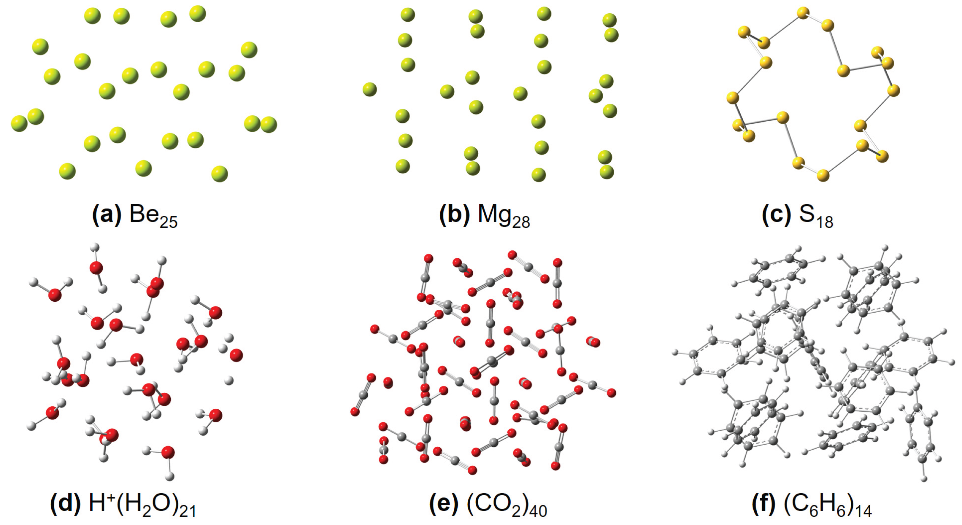
Figure 5.
Comparison of the LR(G3)-predicted and GEBF-calculated MP2-level electron correlation energies for benzene clusters (C6H6)n (n = 15 ‒ 30).
Figure 5.
Comparison of the LR(G3)-predicted and GEBF-calculated MP2-level electron correlation energies for benzene clusters (C6H6)n (n = 15 ‒ 30).
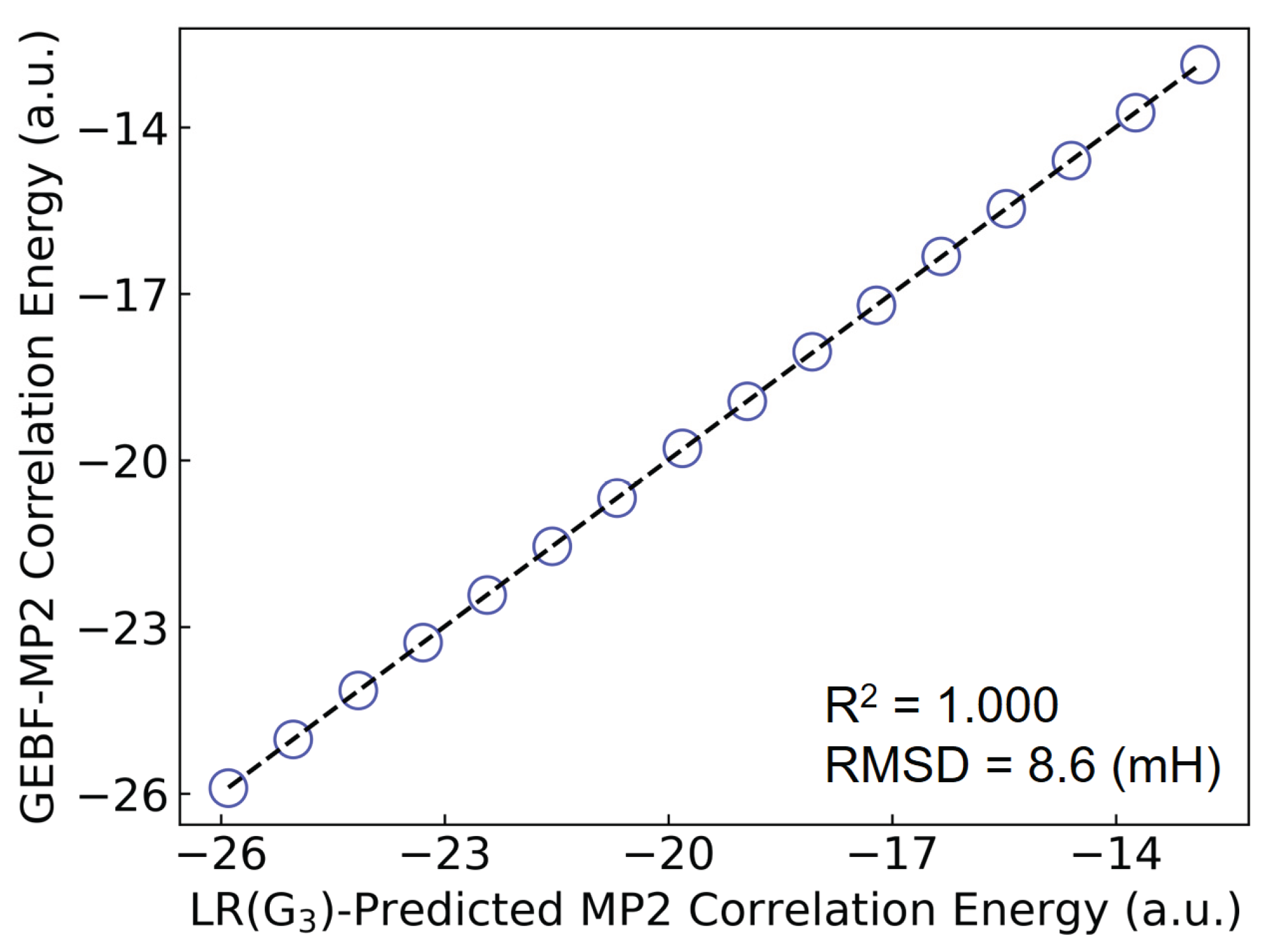

Table 1.
Strong linear correlations (R2) and RMSDa (in mH) between the calculatedb and predicted correlation energies based on the ITA quantitiesc for octane isomers.
Table 1.
Strong linear correlations (R2) and RMSDa (in mH) between the calculatedb and predicted correlation energies based on the ITA quantitiesc for octane isomers.
| ITA | Method | Slope | Intercept | R2 | RMSD |
|---|---|---|---|---|---|
| MP2 | 0.03673221 | ‒4.47037893 | 0.878 | 1.9 | |
| CCSD | 0.02760739 | ‒3.77240773 | 0.897 | 1.3 | |
| CCSD(T) | 0.03224137 | ‒4.22658251 | 0.893 | 1.5 | |
| MP2 | 0.01016369 | ‒21.9076991 | 0.987 | 0.6 | |
| CCSD | 0.00756499 | ‒16.7278042 | 0.989 | 0.4 | |
| CCSD(T) | 0.00885171 | ‒19.3909815 | 0.988 | 0.5 | |
| MP2 | 0.03958034 | ‒18.81389475 | 0.964 | 1.0 | |
| CCSD | 0.02958941 | ‒14.48237993 | 0.974 | 0.6 | |
| CCSD(T) | 0.03459737 | ‒16.75258592 | 0.972 | 0.8 |
aRMSD: root mean squared deviation.bThe basis set 6-311++G(d,p) was used. cHF/6-311++G(d,p).
Table 2.
Strong linear relationships (R2) and RMSDa between the calculatedb and predicted correlation energies based on the ITA quantitiesc for polyyne.
Table 2.
Strong linear relationships (R2) and RMSDa between the calculatedb and predicted correlation energies based on the ITA quantitiesc for polyyne.
| n | /103 | /103 | /103 | |||||||
|---|---|---|---|---|---|---|---|---|---|---|
| 1 | 17.116 | 0.503 | 0.096 | 63.341 | 2.251 | 14.478 | 15.411 | ‒6.702 | 13.889 | 0.253 |
| 2 | 27.503 | 0.996 | 0.178 | 126.454 | 4.498 | 26.687 | 28.049 | ‒11.822 | 26.724 | 0.357 |
| 3 | 37.877 | 1.489 | 0.260 | 189.565 | 6.744 | 38.891 | 40.680 | ‒16.946 | 39.589 | 0.458 |
| 4 | 48.238 | 1.982 | 0.342 | 252.682 | 8.991 | 51.093 | 53.301 | ‒22.064 | 52.468 | 0.556 |
| 5 | 58.604 | 2.475 | 0.425 | 315.797 | 11.238 | 63.292 | 65.918 | ‒27.186 | 65.335 | 0.654 |
| 6 | 68.968 | 2.968 | 0.507 | 378.914 | 13.485 | 75.491 | 78.532 | ‒32.303 | 78.206 | 0.751 |
| 7 | 79.331 | 3.461 | 0.589 | 442.032 | 15.731 | 87.690 | 91.146 | ‒37.422 | 91.079 | 0.849 |
| 8 | 89.696 | 3.954 | 0.671 | 505.147 | 17.978 | 99.888 | 103.759 | ‒42.541 | 103.952 | 0.946 |
| 9 | 100.063 | 4.447 | 0.753 | 568.264 | 20.225 | 112.086 | 116.372 | ‒47.659 | 116.821 | 1.043 |
| 10 | 110.435 | 4.940 | 0.835 | 631.378 | 22.472 | 124.284 | 128.984 | ‒52.780 | 129.686 | 1.139 |
| 30 | 317.730 | 14.800 | 2.478 | 1893.708 | 67.408 | 368.246 | 381.243 | ‒155.141 | 387.180 | 3.076 |
| R 2 | 1.000 | 1.000 | 1.000 | 1.000 | 1.000 | 1.000 | 1.000 | 1.000 | 1.000 | 1.000 |
| RMSD | 1.5 | 1.3 | 1.3 | 1.2 | 1.2 | 1.3 | 1.5 | 1.4 | 0.9 | 2.9 |
aRMSD: root mean squared deviation.bMP2/6-311++G(d,p). cHF/6-311++G(d,p).
Table 3.
Strong linear relationships (R2) and RMSDa between the calculatedb and predicted correlation energies based on the ITA quantitiesc for polyene.
Table 3.
Strong linear relationships (R2) and RMSDa between the calculatedb and predicted correlation energies based on the ITA quantitiesc for polyene.
| n | /103 | /103 | /103 | ||||||
|---|---|---|---|---|---|---|---|---|---|
| 1 | 22.069 | 0.510 | 0.109 | 63.427 | 2.243 | 16.638 | 17.935 | ‒8.846 | 18.948 |
| 2 | 37.486 | 1.010 | 0.204 | 126.732 | 4.489 | 31.067 | 33.236 | ‒16.196 | 37.205 |
| 3 | 52.876 | 1.510 | 0.298 | 189.930 | 6.726 | 45.493 | 48.534 | ‒23.495 | 55.289 |
| 4 | 68.260 | 2.009 | 0.393 | 253.162 | 8.967 | 59.918 | 63.824 | ‒30.808 | 73.409 |
| 5 | 83.643 | 2.509 | 0.488 | 316.406 | 11.209 | 74.342 | 79.111 | ‒38.125 | 91.575 |
| 6 | 99.023 | 3.009 | 0.583 | 379.653 | 13.451 | 88.766 | 94.397 | ‒45.438 | 109.749 |
| 7 | 114.403 | 3.509 | 0.677 | 442.902 | 15.693 | 103.190 | 109.682 | ‒52.756 | 127.925 |
| 8 | 129.783 | 4.008 | 0.772 | 506.150 | 17.934 | 117.613 | 124.967 | ‒60.070 | 146.103 |
| 9 | 145.163 | 4.508 | 0.867 | 569.399 | 20.176 | 132.037 | 140.251 | ‒67.385 | 164.282 |
| 10 | 160.542 | 5.008 | 0.962 | 632.647 | 22.418 | 146.460 | 155.536 | ‒74.701 | 182.461 |
| 30 | 468.132 | 15.003 | 2.856 | 1897.616 | 67.253 | 434.930 | 461.224 | ‒221.004 | 546.043 |
| R 2 | 1.000 | 1.000 | 1.000 | 1.000 | 1.000 | 1.000 | 1.000 | 1.000 | 1.000 |
| RMSD | 2.9 | 2.7 | 2.7 | 2.7 | 2.7 | 2.8 | 3.0 | 2.9 | 2.4 |
aRMSD: root mean squared deviation.bMP2/6-311++G(d,p). cHF/6-311++G(d,p).
Table 4.
Strong linear relationships (R2) and RMSDa between the calculatedb and predicted correlation energies based on the ITA quantitiesc for all-trans-polymethineimine.
Table 4.
Strong linear relationships (R2) and RMSDa between the calculatedb and predicted correlation energies based on the ITA quantitiesc for all-trans-polymethineimine.
| n | /103 | /103 | ||||||
|---|---|---|---|---|---|---|---|---|
| 1 | 17.891 | 0.602 | 0.109 | 84.234 | 4.138 | 16.585 | 17.767 | 17.765 |
| 2 | 29.226 | 1.194 | 0.204 | 168.281 | 8.272 | 30.918 | 32.784 | 35.058 |
| 3 | 40.534 | 1.786 | 0.300 | 252.322 | 12.406 | 45.247 | 47.797 | 52.420 |
| 4 | 51.834 | 2.377 | 0.395 | 336.418 | 16.546 | 59.576 | 62.805 | 69.772 |
| 5 | 63.128 | 2.969 | 0.490 | 420.432 | 20.675 | 73.905 | 77.814 | 87.181 |
| 6 | 74.418 | 3.561 | 0.585 | 504.457 | 24.806 | 88.234 | 92.823 | 104.601 |
| 7 | 85.706 | 4.152 | 0.680 | 588.488 | 28.940 | 102.564 | 107.833 | 121.973 |
| 8 | 96.990 | 4.744 | 0.775 | 672.535 | 33.072 | 116.894 | 122.845 | 139.422 |
| 9 | 108.273 | 5.336 | 0.871 | 756.623 | 37.210 | 131.224 | 137.857 | 156.850 |
| 10 | 119.552 | 5.927 | 0.966 | 840.677 | 41.345 | 145.555 | 152.870 | 174.241 |
| 20 | 232.308 | 11.844 | 1.917 | 1681.135 | 82.670 | 288.867 | 303.008 | 348.833 |
| 30 | 345.014 | 17.761 | 2.869 | 2521.373 | 123.976 | 432.195 | 453.192 | 523.649 |
| R 2 | 1.000 | 1.000 | 1.000 | 1.000 | 1.000 | 1.000 | 1.000 | 1.000 |
| RMSD | 0.4 | 1.0 | 0.9 | 0.9 | 0.7 | 1.1 | 1.2 | 3.9 |
aRMSD: root mean squared deviation.bMP2/6-311++G(d,p). cHF/6-311++G(d,p).
Table 5.
Strong linear relationships (R2) and RMSDa between the calculatedb and predicted correlation energies based on the ITA quantitiesc for acene.
Table 5.
Strong linear relationships (R2) and RMSDa between the calculatedb and predicted correlation energies based on the ITA quantitiesc for acene.
| n | /103 | /103 | /103 | /103 | ||||||
|---|---|---|---|---|---|---|---|---|---|---|
| 2 | 70.395 | 2.489 | 0.460 | 0.316 | 11.207 | 69.910 | 73.784 | ‒34.722 | 25.645 | 88.981 |
| 3 | 94.598 | 3.478 | 0.636 | 0.442 | 15.688 | 96.553 | 101.740 | ‒47.666 | 35.408 | 123.979 |
| 4 | 118.807 | 4.468 | 0.811 | 0.569 | 20.169 | 123.195 | 129.691 | ‒60.602 | 45.077 | 158.965 |
| 5 | 143.022 | 5.457 | 0.987 | 0.695 | 24.651 | 149.835 | 157.637 | ‒73.547 | 54.729 | 193.946 |
| 6 | 167.241 | 6.447 | 1.162 | 0.821 | 29.133 | 176.474 | 185.576 | ‒86.480 | 64.373 | 228.921 |
| 7 | 191.461 | 7.436 | 1.338 | 0.948 | 33.614 | 203.111 | 213.512 | ‒99.419 | 74.020 | 263.894 |
| 8 | 215.675 | 8.426 | 1.513 | 1.074 | 38.096 | 229.747 | 241.444 | ‒112.348 | 83.657 | 298.878 |
| 9 | 239.894 | 9.415 | 1.689 | 1.200 | 42.578 | 256.382 | 269.372 | ‒125.278 | 93.298 | 333.853 |
| 10 | 264.114 | 10.405 | 1.865 | 1.326 | 47.059 | 283.016 | 297.298 | ‒138.209 | 102.944 | 368.828 |
| 11 | 288.484 | 11.394 | 2.040 | 1.453 | 51.543 | 309.627 | 325.167 | ‒151.260 | 112.708 | 404.117 |
| R2 | 1.000 | 1.000 | 1.000 | 1.000 | 1.000 | 1.000 | 1.000 | 1.000 | 1.000 | 1.000 |
| RMSD | 10.5 | 11.5 | 11.4 | 11.4 | 11.4 | 11.6 | 11.9 | 10.4 | 10.9 | 10.3 |
aRMSD: root mean squared deviation.bMP2/6-311++G(d,p). cHF/6-311++G(d,p).
Table 6.
Strong linear relationships (R2) and RMSDa between the calculatedb and predicted correlation energies based on the ITA quantitiesc for neutral Ben (n = 3 ‒ 25) clusters.
Table 6.
Strong linear relationships (R2) and RMSDa between the calculatedb and predicted correlation energies based on the ITA quantitiesc for neutral Ben (n = 3 ‒ 25) clusters.
| R2 | 0.996 | 0.996 | 0.996 | 0.996 | 0.996 | 0.994 | 0.993 |
| RMSD | 28.5 | 28.6 | 27.9 | 28.0 | 27.9 | 35.9 | 37.1 |
aRMSD: root mean squared deviation.bMP2/6-311++G(d,p). cHF/6-311++G(d,p).
Table 7.
Strong linear relationships (R2) and RMSDa between the calculatedb and predicted correlation energies based on the ITA quantitiesc for Mgn (n = 3 ‒ 20, and 28) clusters.
Table 7.
Strong linear relationships (R2) and RMSDa between the calculatedb and predicted correlation energies based on the ITA quantitiesc for Mgn (n = 3 ‒ 20, and 28) clusters.
| /103 | /103 | /103 | /105 | |||||
|---|---|---|---|---|---|---|---|---|
| R2 | 0.998 | 0.996 | 0.996 | 0.996 | 0.996 | 0.995 | 0.993 | 0.995 |
| RMSD | 17.7 | 24.8 | 25.2 | 24.8 | 24.8 | 26.7 | 33.0 | 27.2 |
aRMSD: root mean squared deviation.bMP2/6-311++G(d,p). cHF/6-311++G(d,p).
Table 8.
Strong linear relationships (R2) and RMSDa between the calculatedb and predicted correlation energies based on the ITA quantitiesc for covalent Sn (n = 2 ‒ 18) clusters. .
Table 8.
Strong linear relationships (R2) and RMSDa between the calculatedb and predicted correlation energies based on the ITA quantitiesc for covalent Sn (n = 2 ‒ 18) clusters. .
| /103 | /103 | /103 | /106 | |||||
|---|---|---|---|---|---|---|---|---|
| R2 | 0.998 | 0.998 | 0.998 | 0.998 | 0.998 | 0.998 | 0.998 | 0.995 |
| RMSD | 29.5 | 26.9 | 26.7 | 26.9 | 26.9 | 27.7 | 29.5 | 42.2 |
aRMSD: root mean squared deviation.bMP2/6-311++G(d,p). cHF/6-311++G(d,p).
Table 9.
Strong linear correlations and RMSDa between the calculatedb and predicted correlation energies based on the ITA quantitiesc for protonated water clusters.
Table 9.
Strong linear correlations and RMSDa between the calculatedb and predicted correlation energies based on the ITA quantitiesc for protonated water clusters.
| ITA | Slope | Intercept | R2 | RMSD (mH) |
|---|---|---|---|---|
| ‒0.03129182 | 0.00240752 | 1.000 | 4.2 | |
| ‒0.00049499 | 0.01775234 | 1.000 | 2.2 | |
| ‒0.00332260 | 0.01628422 | 1.000 | 2.2 | |
| ‒0.00279107 | 0.01637182 | 1.000 | 2.1 | |
| ‒3.24672546×10‒5 | 1.58843194×10‒2 | 1.000 | 2.1 | |
| ‒0.02186241 | 0.00482623 | 1.000 | 3.0 | |
| ‒0.02042257 | ‒0.00317343 | 1.000 | 6.8 | |
| ‒0.01981287 | 0.03859503 | 1.000 | 9.3 |
aRMSD: root mean squared deviation. bMP2/6-311++G(d,p). cHF/6-311++G(d,p).
Table 10.
Strong linear relationships (R2) and RMSDa between the calculatedb and predicted correlation energies based on the ITA quantitiesc for CO2 clusters. .
Table 10.
Strong linear relationships (R2) and RMSDa between the calculatedb and predicted correlation energies based on the ITA quantitiesc for CO2 clusters. .
| n | /103 | /103 | /103 | /105 | ||||
|---|---|---|---|---|---|---|---|---|
| 4 | 35.676 | 4.618 | 0.604 | 0.777 | 0.608 | 90.119 | 94.242 | 87.199 |
| 5 | 44.343 | 5.772 | 0.755 | 0.972 | 0.760 | 112.597 | 117.629 | 110.311 |
| 6 | 52.975 | 6.925 | 0.905 | 1.166 | 0.911 | 135.124 | 141.177 | 133.364 |
| 7 | 61.551 | 8.078 | 1.056 | 1.360 | 1.063 | 157.664 | 164.803 | 156.231 |
| 8 | 70.225 | 9.232 | 1.207 | 1.555 | 1.215 | 180.182 | 188.320 | 179.164 |
| 9 | 78.890 | 10.385 | 1.357 | 1.749 | 1.367 | 202.688 | 211.805 | 202.144 |
| 10 | 87.459 | 11.538 | 1.508 | 1.943 | 1.519 | 225.201 | 235.323 | 225.314 |
| 11 | 96.066 | 12.691 | 1.659 | 2.138 | 1.671 | 247.744 | 258.928 | 248.319 |
| 12 | 104.630 | 13.845 | 1.810 | 2.332 | 1.823 | 270.253 | 282.434 | 271.861 |
| 13 | 113.096 | 14.997 | 1.960 | 2.526 | 1.975 | 292.762 | 305.941 | 295.591 |
| 14 | 121.760 | 16.151 | 2.111 | 2.721 | 2.127 | 315.271 | 329.437 | 318.380 |
| 15 | 130.261 | 17.303 | 2.262 | 2.915 | 2.279 | 337.783 | 352.939 | 342.101 |
| 16 | 138.809 | 18.456 | 2.412 | 3.110 | 2.431 | 360.299 | 376.486 | 365.340 |
| 17 | 147.426 | 19.610 | 2.563 | 3.304 | 2.582 | 382.823 | 400.036 | 388.562 |
| 18 | 155.935 | 20.763 | 2.714 | 3.498 | 2.734 | 405.331 | 423.523 | 411.987 |
| 19 | 164.464 | 21.916 | 2.864 | 3.692 | 2.886 | 427.851 | 447.048 | 435.461 |
| 20 | 173.049 | 23.069 | 3.015 | 3.887 | 3.039 | 450.351 | 470.533 | 458.492 |
| 21 | 181.681 | 24.222 | 3.166 | 4.081 | 3.190 | 472.899 | 494.173 | 481.566 |
| 22 | 190.085 | 25.375 | 3.316 | 4.275 | 3.342 | 495.391 | 517.595 | 505.485 |
| 23 | 198.669 | 26.528 | 3.467 | 4.275 | 3.342 | 517.900 | 541.108 | 528.669 |
| 24 | 207.333 | 27.681 | 3.618 | 4.470 | 3.494 | 540.447 | 564.742 | 551.542 |
| 25 | 215.912 | 28.834 | 3.768 | 4.664 | 3.645 | 562.977 | 588.305 | 575.132 |
| 26 | 224.348 | 29.987 | 3.919 | 4.858 | 3.797 | 585.450 | 611.697 | 598.457 |
| 27 | 232.942 | 31.140 | 4.069 | 5.053 | 3.950 | 607.998 | 635.332 | 621.629 |
| 28 | 241.311 | 32.292 | 4.220 | 5.247 | 4.102 | 630.486 | 658.742 | 646.216 |
| 29 | 249.849 | 33.445 | 4.371 | 5.441 | 4.253 | 653.028 | 682.370 | 669.245 |
| 30 | 258.485 | 34.598 | 4.521 | 5.636 | 4.405 | 675.542 | 705.876 | 692.513 |
| 31 | 266.924 | 35.751 | 4.672 | 5.830 | 4.557 | 698.031 | 729.325 | 716.064 |
| 32 | 275.455 | 36.904 | 4.823 | 6.025 | 4.709 | 720.528 | 752.779 | 739.801 |
| 33 | 283.987 | 38.057 | 4.973 | 6.219 | 4.861 | 743.042 | 776.303 | 763.194 |
| 34 | 292.460 | 39.209 | 5.124 | 6.413 | 5.013 | 765.584 | 799.882 | 786.656 |
| 35 | 301.250 | 40.363 | 5.275 | 6.608 | 5.165 | 788.149 | 823.593 | 809.202 |
| 36 | 309.838 | 41.516 | 5.425 | 6.802 | 5.316 | 810.635 | 847.024 | 832.618 |
| 37 | 318.350 | 42.669 | 5.576 | 7.191 | 5.620 | 833.121 | 870.410 | 856.497 |
| 38 | 326.874 | 43.822 | 5.727 | 7.385 | 5.772 | 855.667 | 894.049 | 879.546 |
| 39 | 335.361 | 44.974 | 5.877 | 7.579 | 5.924 | 878.154 | 917.451 | 903.378 |
| 40 | 343.794 | 46.127 | 6.028 | 7.774 | 6.076 | 900.680 | 941.037 | 927.399 |
| R2 | 1.000 | 1.000 | 1.000 | 1.000 | 1.000 | 1.000 | 1.000 | 1.000 |
| RMSD | 14.6 | 6.5 | 6.6 | 6.3 | 6.3 | 6.4 | 6.8 | 10.8 |
aRMSD: root mean squared deviation.bMP2/6-311++G(d,p). cHF/6-311++G(d,p).
Table 11.
Strong linear relationships (R2) and RMSDa between the calculatedb and predicted correlation energies based on the ITA quantitiesc for benzene (C6H6)n clusters. .
Table 11.
Strong linear relationships (R2) and RMSDa between the calculatedb and predicted correlation energies based on the ITA quantitiesc for benzene (C6H6)n clusters. .
| n | /103 | /103 | /103 | ||||||
|---|---|---|---|---|---|---|---|---|---|
| 4 | 182.943 | 5.993 | 1.136 | 759.350 | 26.923 | 172.970 | 183.096 | ‒87.149 | 221.627 |
| 5 | 228.316 | 7.490 | 1.420 | 948.919 | 33.629 | 216.208 | 228.869 | ‒108.820 | 277.997 |
| 6 | 273.691 | 8.987 | 1.703 | 1138.819 | 40.367 | 259.454 | 274.657 | ‒130.621 | 334.386 |
| 7 | 318.886 | 10.483 | 1.987 | 1328.458 | 47.078 | 302.685 | 320.404 | ‒152.252 | 391.102 |
| 8 | 364.310 | 11.980 | 2.270 | 1518.321 | 53.807 | 345.919 | 366.163 | ‒174.079 | 447.714 |
| 9 | 409.374 | 13.477 | 2.554 | 1708.000 | 60.526 | 389.160 | 411.955 | ‒195.780 | 504.763 |
| 10 | 454.744 | 14.974 | 2.838 | 1897.903 | 67.261 | 432.383 | 457.676 | ‒217.571 | 561.267 |
| 11 | 500.069 | 16.471 | 3.121 | 2087.468 | 73.973 | 475.630 | 503.477 | ‒239.230 | 617.793 |
| 12 | 545.054 | 17.967 | 3.404 | 2277.421 | 80.708 | 518.879 | 549.286 | ‒261.020 | 675.525 |
| 13 | 589.963 | 19.462 | 3.688 | 2467.339 | 87.442 | 562.104 | 595.025 | ‒282.767 | 733.570 |
| 14 | 635.264 | 20.959 | 3.971 | 2656.842 | 94.148 | 605.328 | 640.753 | ‒304.418 | 789.848 |
| R2 | 1.000 | 1.000 | 1.000 | 1.000 | 1.000 | 1.000 | 1.000 | 1.000 | 1.000 |
| RMSD | 10.7 | 7.6 | 7.7 | 7.1 | 6.9 | 7.3 | 7.3 | 7.5 | 2.8 |
aRMSD: root mean squared deviation. bMP2/6-311++G(d,p). cHF/6-311++G(d,p).
Disclaimer/Publisher’s Note: The statements, opinions and data contained in all publications are solely those of the individual author(s) and contributor(s) and not of MDPI and/or the editor(s). MDPI and/or the editor(s) disclaim responsibility for any injury to people or property resulting from any ideas, methods, instructions or products referred to in the content. |
© 2025 by the authors. Licensee MDPI, Basel, Switzerland. This article is an open access article distributed under the terms and conditions of the Creative Commons Attribution (CC BY) license (http://creativecommons.org/licenses/by/4.0/).
Copyright: This open access article is published under a Creative Commons CC BY 4.0 license, which permit the free download, distribution, and reuse, provided that the author and preprint are cited in any reuse.


