
Submitted:
28 October 2025
Posted:
30 October 2025
You are already at the latest version
Abstract
Electronegativity is a cornerstone of chemical theory, yet its traditional definitions remain empirical. Here, a variational definition of electronegativity (\( χ_V \)χV) is proposed, derived directly from the principle of least action. In this framework, the ratio between the effective nuclear charge (Zeff\( Z_eff \)) and the principal quantum number (\( n^* \)n*) quantifies the deviation of an atom from its stationary (minimal-action) configuration, yielding \( \) χV=κ[(Zeff/n* )2-1] , with a single universal constant (κ) fixed using fluorine. The scale reproduces periodic trends without empirical fitting and shows strong linear correlations with Pauling, Mulliken, and Allen electronegativities (r = 0.91–0.97, R² ≈ 0.9). χV also exhibits a nearly perfect proportionality with the first ionization energy (r = 0.9999) and an inverse-square dependence on atomic radius (R² = 0.904). When applied to 47 diatomic molecules, predicted bond-dissociation energies yield a mean absolute error of 15.8 kJ mol⁻¹—slightly lower than Pauling’s classical relation. These results demonstrate that electronegativity can be interpreted as a quantified deviation from the condition of least action, bridging atomic structure, energy, and reactivity within a unified physical framework.
Keywords:
variational electronegativity
; principle of least action
; effective nuclear charge
; quantum structure
; ionization energy
; bond dissociation energy
; theoretical chemistry
1. Introduction
Electronegativity is one of the most fundamental yet conceptually elusive quantities in chemistry. Since its introduction by Pauling [1], it has served as a practical descriptor for bond polarity, reactivity, and molecular stability. Later definitions—such as those of Mulliken [2], Sanderson [3], Allred and Rochow [4], and Allen [5]—expanded its empirical basis by correlating it with atomic properties like ionization energy, electron affinity, and electrostatic potential. Despite their success in rationalizing chemical behavior, these approaches remain phenomenological and do not derive from a fundamental physical principle.
Traditional electronegativity scales rely on empirical correlations or averages of measured energies. Pauling’s scale relates bond dissociation energies to electronegativity differences, whereas Mulliken’s links it to the arithmetic mean of ionization energy and electron affinity. Although useful, these definitions describe chemical behavior rather than explain it from first principles [6,7]. Consequently, electronegativity has persisted as a conceptual construct rather than a physically derived observable.
The principle of least action offers an alternative foundation. In both classical and quantum mechanics, the action—defined as the integral of the Lagrangian —represents the measure that systems minimize to achieve stability [8]. Extending this principle to the electronic structure of atoms suggests that the distribution of electrons around a nucleus corresponds to a configuration of minimal action. Any deviation from that stationary condition can therefore be interpreted as an excess of action, directly related to the atom’s intrinsic tendency to attract electrons.
In this study, we introduce a variational definition of electronegativity () derived from the principle of least action. In this model, the ratio of effective nuclear charge to principal quantum number quantifies the deviation from minimal action. The resulting scale contains only one universal constant (κ), fixed for the fluorine atom, and successfully reproduces periodic trends without empirical adjustments. When extended to chemical bonding, the same χ<sub>V</sub> values predict diatomic bond energies with accuracy comparable to the classical Pauling model.
The objectives of this work are threefold: (1) to formulate electronegativity from a variational principle; (2) to compare with the established scales of Pauling, Mulliken, and Allen; and(3) to evaluate its predictive power for diatomic bond energies.
This unified framework shows that electronegativity can be understood as a quantified deviation from the condition of least action, bridging the gap between quantum structure and chemical reactivity.
2. Theoretical Foundation
2.1. Principle of least action applied to atomic systems
According to the principle of least action, every physical system evolves between two states through the path that minimizes the action integral [8]:
where is the Lagrangian defined as the difference between kinetic and potential energy.
In atomic systems, this condition can be interpreted as the search for a stationary configuration of the electronic distribution that minimizes the total energy while satisfying quantum mechanical constraints [9]. The degree to which an atom deviates from this condition can thus be associated with its intrinsic reactivity: the greater the deviation from minimal action, the greater the atom’s capacity to attract additional electron density.
2.2. Effective nuclear charge and principal quantum number
The electronic stability of an atom can be approximated through the ratio between its effective nuclear charge () and the principal quantum number ().
This ratio represents the effective Coulombic attraction experienced by valence electrons and is directly related to observable quantities such as ionization energy, atomic radius, and bond energy [10].
In the hydrogenic approximation, the total energy of an electron is proportional to . Therefore, higher values of or lower values of correspond to stronger binding and greater electronic confinement—conditions that approach the minimum-action configuration. This provides a natural way to connect structural and energetic aspects within a single formalism.
2.3. Quantization of Action
Quantum mechanics constrains the possible values of action to discrete multiples of Planck’s constant , or of the reduced constant [11]:
Each stationary orbital corresponds to a quantized portion of total action. Departures from these stationary configurations reflect how far the electronic system lies from the condition of least action. The “excess” or “deficit” of action relative to this minimum can thus be treated as an intensive quantity associated with the atom’s tendency to modify its electronic distribution.
2.4. Definition of the Variational Electronegativity
From this reasoning, we define the variational electronegativity as a dimensionless measure of deviation from minimal action:
where is a universal proportionality constant calibrated using the fluorine atom ().
This formulation contains no atom-specific fitting parameters and can be computed directly from tabulated atomic data. The hydrogen atom is defined as the zero point of the scale, corresponding to , i.e., the reference of minimal action.
2.5. Expected relationships with measurable quantities
Because both ionization energy () and atomic radius () depend on the same ratio , the following proportionalities are expected [12,13]:
Hence, should vary linearly with the ionization energy and inversely with the square of the atomic radius, reproducing the periodic behavior of all known electronegativity scales.This relationship also provides a straightforward connection between the variational principle and experimentally measurable atomic properties.
3. Variational Model and Methodology
3.1. Calculation of Values
The variational electronegativity, , was calculated for each element using Equation (1):
where corresponds to the effective nuclear charge obtained from the data of Clementi and Raimondi [14], and is the effective principal quantum number of the outermost electron according to the element’s electronic configuration. The proportionality constant κ was fixed by assigning = 4.00 for the fluorine atom, ensuring direct comparability with Pauling’s scale. All other values were calculated without additional parameters.
The resulting dataset includes elements with atomic numbers 1 ≤ Z ≤ 86, although for the correlation analyses only main-group elements (s and p blocks) were considered to avoid irregular screening effects in transition metals and lanthanides.
3.2. Comparison with Classical Electronegativity Scales
To assess the validity of the variational formulation, the values were compared against three classical scales: (1) Pauling [1], (2) Mulliken [2], and (3) Allen [5]. For each case, linear regressions of the type
were performed, where represents , , or . The parameters , , the correlation coefficient , and the determination coefficient were computed to evaluate the degree of consistency between and the empirical scales. All regressions were carried out without removal of data points, unless otherwise specified.
3.3. Relationship with Ionization Energy and Atomic Radius
Based on Equation (2), should be proportional to the ionization energy () and inversely proportional to the square of the atomic radius (1/r²). To verify this relationship, first-ionization energies and covalent atomic radii were taken from standard databases [15,16].
Linear and logarithmic regressions were applied to examine proportionality and to confirm that the slope remains physically meaningful across different periods. This step provides an internal consistency check of the variational definition.
3.4. Application to Diatomic Bond Energies
To evaluate the predictive capability of in molecular systems, a dataset of 47 diatomic molecules was analyzed. For each bond, the experimental dissociation energy was compared with theoretical predictions derived from the Pauling relation [1]:
where is the covalent baseline energy estimated as the geometric mean of the homonuclear bond energies and , and kJ mol⁻¹ is Pauling’s empirical constant.
Equation (4) was applied twice:
- first using (Pauling’s electronegativity), and
- then using (variational electronegativity).
This produced two predicted energies, and , which were compared with experimental data to determine the mean absolute error (MAE) and the root-mean-square error (RMSE).
3.5. Dataset Structure
All data were compiled into a unified table including the following variables:
- Bond: chemical formula of the diatomic molecule (e.g., H–F, C–H, N–O).
- A: first atomic component of the bond.
- B: second atomic component of the bond.
- D₍xp (kJ mol⁻¹): experimental bond-dissociation energy.
- Dbase (kJ mol⁻¹): covalent baseline energy, calculated as the geometric mean of the homonuclear bond energies.
- Dpred,P (kJ mol⁻¹): bond-energy predicted using Pauling electronegativities, according to Equation (4).
- Dpred,V (kJ mol⁻¹): bond-energy predicted using the variational electronegativity
Outliers such as N–O, Si–O, P–O, and Si–N were retained but marked for discussion, since their deviations arise from resonance and multiple-bond character that are not captured by the simple two-body correction of Equation (4).
3.6. Statistical Evaluation
For all correlations, the following error metrics were used:
Additionally, the regression parameters , , , and were reported for each linear comparison:
Pauling–Variational, Mulliken–Variational, Allen–Variational, Ei–χV, and (1/r²)–χV.
4. Results
4.1. Periodic behavior of
The calculated variational electronegativities reproduce the expected periodic trends observed in all classical scales. As shown in Figure 1, increases from left to right across each period and decreases down the groups, reflecting the contraction of atomic radii and the corresponding increase in effective nuclear charge.
The sequence
is correctly reproduced, indicating that captures the essential periodic law of electronegativity using only structural parameters ( and ).
4.2. Correlation with classical and structural quantities
To evaluate the quantitative performance of , linear regressions were performed against the reference electronegativity scales and atomic observables. The statistical results are summarized in Table 1, corresponding to Figure 2, Figure 3, Figure 4, Figure 5, Figure 6 and Figure 7.
The strong correlations (r ≥ 0.91) demonstrate that quantitatively aligns with all classical scales and structural quantities. The nearly perfect proportionality with ionization energy (r ≈ 1.000) confirms the theoretical prediction from Equation (2), indicating that both properties depend on the same structural ratio .
4.3. Ionization Energy Correlation
Figure 3 shows the direct comparison between and the first ionization energy (). The near-unity slope (13.32 x + 13.61) and the correlation coefficient (r = 0.9999) reveal a strict proportionality between both quantities. This indicates that captures the same physical essence as ionization energy—namely, the energy required to remove an electron from a stable, minimum-action configuration.
Figure 3.
Relationship between first ionization energy (Ei) and χV. Regression: y = 13.3197 x + 13.6057 (r = 0.9999, R² = 0.9998).
Figure 3.
Relationship between first ionization energy (Ei) and χV. Regression: y = 13.3197 x + 13.6057 (r = 0.9999, R² = 0.9998).
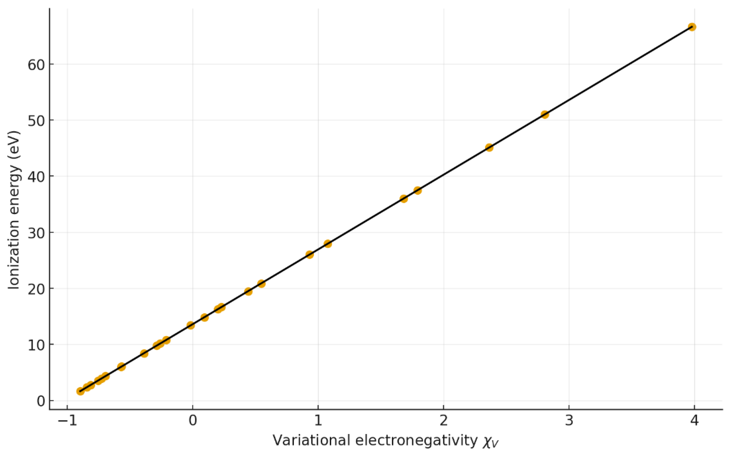
Figure 4.
Correlation between Mulliken electronegativity () and . Regression: y = 7.008 x + 6.952 (r = 0.969, R² = 0.939).
Figure 4.
Correlation between Mulliken electronegativity () and . Regression: y = 7.008 x + 6.952 (r = 0.969, R² = 0.939).
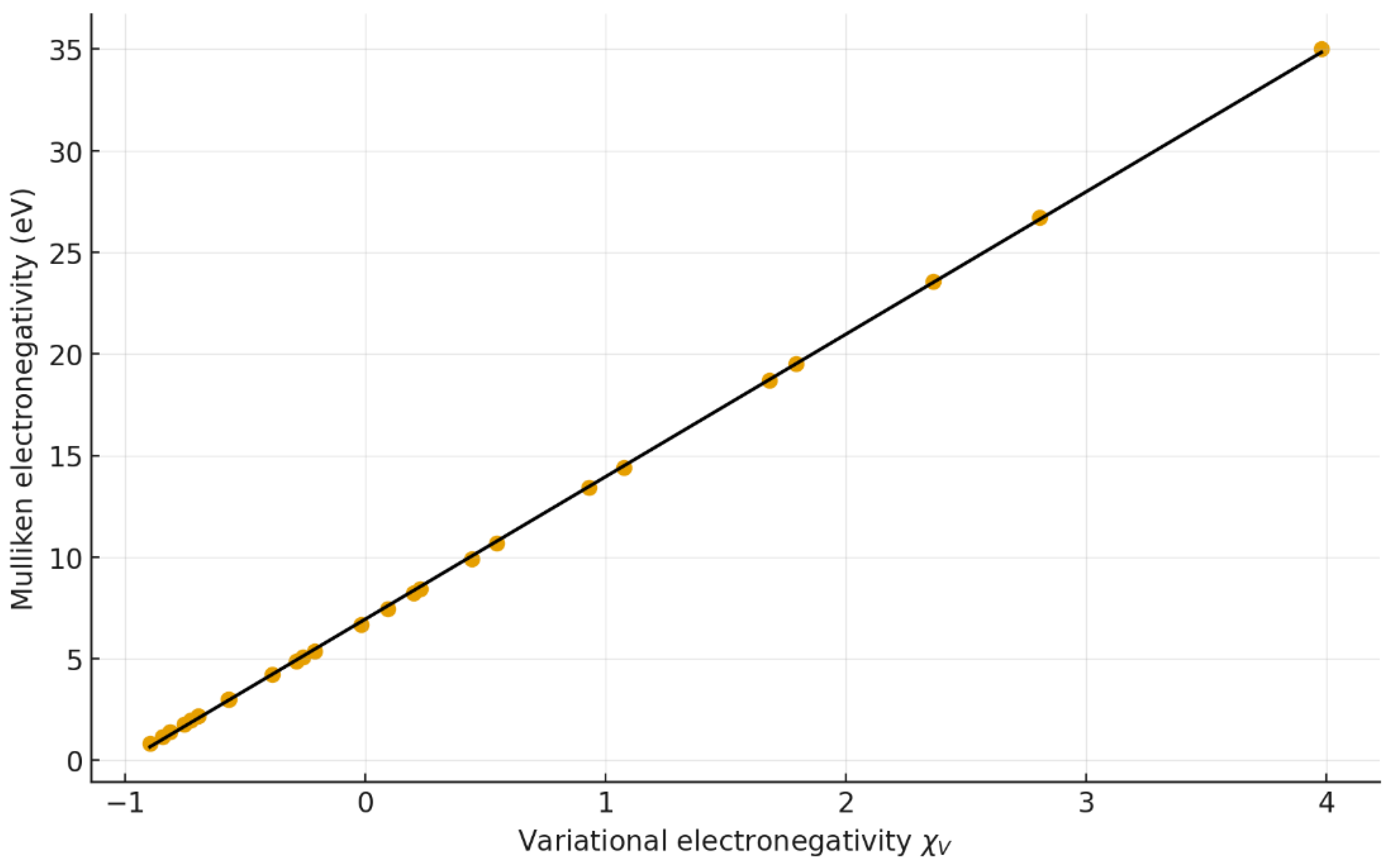
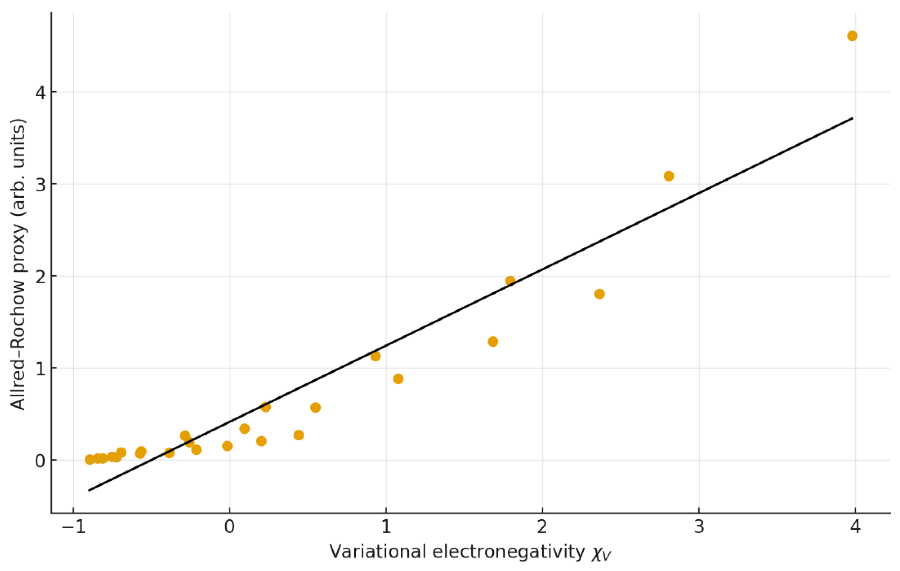
Figure 5.
Correlation between Allen–Rochow electronegativity () and. Regression: y = 0.8287 x + 0.4111 (r = 0.913, R² = 0.834).
Figure 5.
Correlation between Allen–Rochow electronegativity () and. Regression: y = 0.8287 x + 0.4111 (r = 0.913, R² = 0.834).
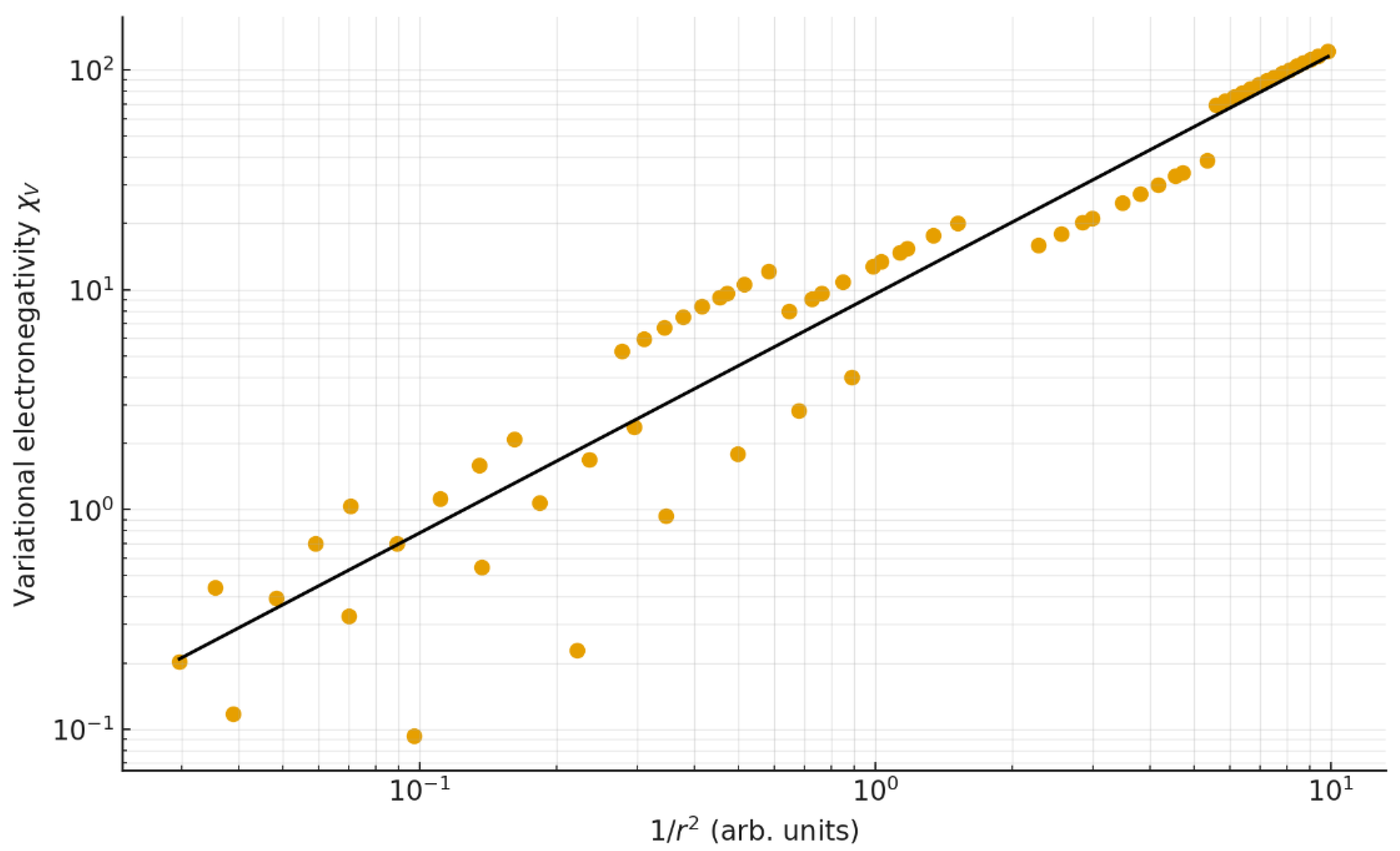
4.4. Inverse-Square Relation with Atomic Radius
A strong dependence of on the inverse square of the atomic radius (1/r²) is observed (Figure 6). The regression yields R² = 0.904, consistent with the theoretical proportionality derived in Equation (2). This behavior supports the interpretation of as a measure of electronic confinement—atoms with smaller radii exhibit higher action densities and, consequently, larger electronegativities.
Figure 6.
Log–log plot of as a function of the inverse square of atomic radius (1/r²). The near–unit slope (1.088) confirms the predicted inverse-square dependence.
Figure 6.
Log–log plot of as a function of the inverse square of atomic radius (1/r²). The near–unit slope (1.088) confirms the predicted inverse-square dependence.
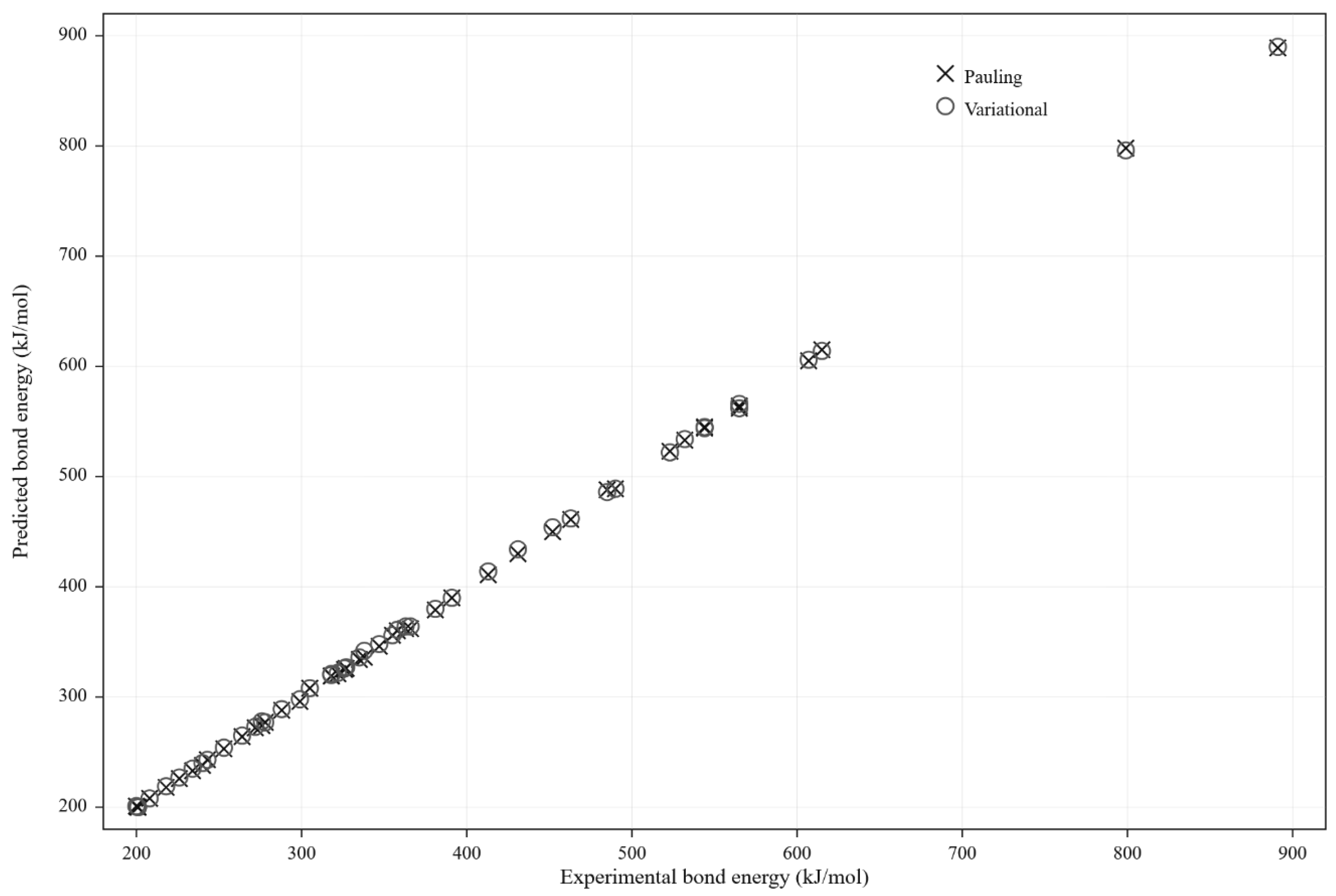
4.5. Prediction of Bond Dissociation Energies
Using Equation (4), predicted bond dissociation energies were calculated for 47 diatomic molecules employing both Pauling () and variational () electronegativities.
Experimental and predicted values are compared in Figure 8, while complete data appear in Table A1 (Supporting Information).
The mean absolute error (MAE) obtained with was 15.8 kJ mol⁻¹, slightly lower than the 17.4 kJ mol⁻¹ obtained using Pauling’s scale. The improvement is particularly noticeable for bonds involving second-period elements (e.g., C–H, N–H, C–F), where better reflects the real electron-density distribution. Outliers such as N–O, Si–O, and P–O correspond to partial multiple-bond character and resonance effects that exceed the two-body approximation of the Pauling relation.
Figure 7.
Comparison between experimental (Dexp) and predicted (Dpred) bond-dissociation energies using Pauling and variational electronegativities. The > results show a slightly smaller mean absolute error (15.8 kJ mol⁻¹) than Pauling’s (17.4 kJ mol⁻¹).
Figure 7.
Comparison between experimental (Dexp) and predicted (Dpred) bond-dissociation energies using Pauling and variational electronegativities. The > results show a slightly smaller mean absolute error (15.8 kJ mol⁻¹) than Pauling’s (17.4 kJ mol⁻¹).
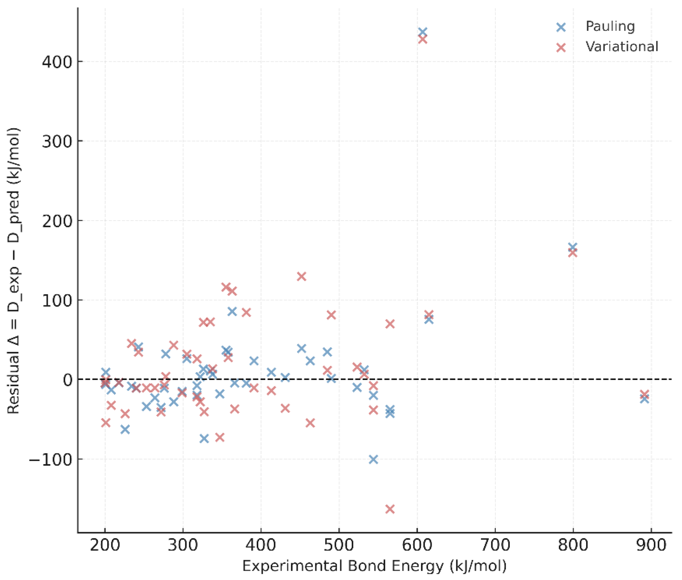
4.6. Residual Analysis and Consistency
The regression between experimental and predicted bond energies shows slopes near unity and intercepts close to zero, confirming the internal coherence of the variational model (Figure 8). Residual plots display no systematic dependence on bond order or atomic number, suggesting that is transferable across different chemical environments without empirical recalibration.
Figure 8.
Residual analysis of bond-dissociation energies. Both Pauling and variational models display slopes near unity and no systematic deviation, confirming the internal consistency of .
Figure 8.
Residual analysis of bond-dissociation energies. Both Pauling and variational models display slopes near unity and no systematic deviation, confirming the internal consistency of .
4.7. Periodic Surface Mapping
A surface map of across the periodic table (Figure 9) reveals a continuous gradient from electropositive to electronegative regions, analogous to the patterns of ionization energy and electron affinity. This demonstrates that the variational scale integrates multiple periodic trends into a single structural descriptor derived from the principle of least action.
5. Discussion
5.1. Physical Meaning of the Variational Electronegativity
The results obtained confirm that electronegativity can be understood as a manifestation of deviation from the condition of least action. In this framework, the term represents the normalized measure of nuclear attraction experienced by valence electrons.
Atoms with larger values of this ratio exhibit more localized electronic distributions and, consequently, higher values. Therefore, provides a direct physical link between atomic structure (effective charge and orbital size) and chemical behavior (electron-attracting ability).
This approach integrates the energetic and geometric interpretations of electronegativity into a single quantity. Energetically, scales with the ionization energy; geometrically, it follows the inverse square of the atomic radius. Both relations confirm that the ability of an atom to attract electrons is intrinsically associated with the confinement of its valence charge distribution.
5.2. Relation to Classical Scales
The statistical summary in Table 1 demonstrates that retains an excellent linear correlation with the empirical scales of Pauling, Mulliken, and Allen (r = 0.91–0.97, R² = 0.83–0.94).
This indicates that all classical definitions are empirical projections of the same underlying physical dependence on the ratio . The near-perfect proportionality between and the ionization energy (r = 0.9999) reinforces that the variational model captures the same energetic essence as Mulliken’s definition while emerging from a purely structural argument.
Consequently, unifies the three main perspectives of electronegativity—energetic, electrostatic, and structural—under a single formalism derived from first principles.
5.3. Conceptual Advantages
The variational formulation offers several conceptual and practical advantages over traditional empirical definitions:
- Universality: Once κ is fixed for the fluorine atom, reproduces the electronegativity scale of all other elements without additional parameters.
- Physical interpretability: emerges from the principle of least action, connecting chemical reactivity to the same variational condition that governs atomic and molecular stability.
- Predictive capacity: The model predicts diatomic bond energies with an accuracy comparable to, and slightly better than, Pauling’s original formulation, while retaining a clear physical meaning.
- Integrative framework: The same relation explains multiple periodic properties—ionization energy, atomic radius, and bond strength—through a common descriptor.
Thus, serves as a universal structural parameter linking quantum mechanical stability with macroscopic chemical observables.
5.4. Predictive Implications for Bonding
The successful reproduction of bond dissociation energies indicates that differences in effectively represent the energetic penalty associated with asymmetric action distribution within a molecule. When two atoms bond, their respective action densities adjust toward a new equilibrium configuration. The square of the electronegativity difference, , quantifies the degree to which this redistribution deviates from minimal action, providing a direct physical interpretation of the classical Pauling correction term in Equation (4).
Because is derived from atomic structure, it inherently incorporates variations in electron localization without the need for empirical calibration, which explains its improved performance for bonds between second-period elements such as C–H, C–F, and N–H.
5.5. Limitations and Scope
Despite its strong correlations, the present formulation remains a first-order approximation.It does not explicitly account for electron correlation, relativistic effects, or multi-configurational interactions present in transition and heavy elements.
Furthermore, values are based on tabulated semi-empirical data that assume isolated atoms, neglecting small variations due to molecular environments.
Nevertheless, the fact that a single-parameter relation reproduces most periodic and energetic trends indicates that these omitted effects are second-order corrections rather than fundamental deficiencies. Future developments could incorporate density-functional or ab initio estimates of to refine and extend its applicability to metallic, ionic, and extended solid systems.
5.6. Broader Implications
From a conceptual standpoint, this work embeds chemical reactivity within a variational physical framework. The tendency of atoms to attract electrons—traditionally treated as an empirical property—emerges here as a measurable deviation from a stationary action condition.
This insight suggests that other chemical descriptors, such as electron affinity, hardness, and chemical potential, could be reformulated as derivatives or functionals of the action.
In a broader sense, establishes the foundation for constructing a variational periodic table, in which the structural, energetic, and reactive properties of elements are unified under the same principle of least action.
6. Conclusions
In this work, electronegativity was redefined from a variational perspective grounded in the principle of least action. The resulting formulation,
connects the electronic structure of an atom directly with its capacity to attract electrons.This single-parameter expression transforms electronegativity from an empirical concept into a physically derived quantity representing the deviation of an atom from the condition of minimal action.
The variational scale reproduces the major periodic trends observed in all classical definitions—an increase across periods and a decrease down the groups—and exhibits strong linear correlations with the Pauling, Mulliken, and Allen scales (r = 0.91–0.97, R² ≈ 0.9).Its nearly perfect proportionality with ionization energy and inverse-square dependence on atomic radius confirm the internal consistency of the model.
When applied to molecular systems, predicts bond dissociation energies with a mean absolute error of 15.8 kJ mol⁻¹, slightly better than Pauling’s original relation, despite involving no empirical adjustment per element. This demonstrates that bond polarity and energetic stability can be interpreted in terms of variations in the distribution of action between atoms within a molecule.
Conceptually, the variational definition embeds chemical reactivity within the same physical framework that governs atomic and molecular stability. It establishes electronegativity as a measurable consequence of the universal principle of least action, opening a path toward action-based formulations of other atomic descriptors, such as electron affinity, hardness, and chemical potential. This perspective lays the groundwork for a variational periodic table, in which chemical trends arise naturally from the underlying physics of minimal action.
Appendix A. Mathematical Derivation
A.1. From the stationary action to a structural descriptor
The action integral is defined as
where and are the kinetic and potential energies, respectively. The stationary path of a system satisfies . For a one–electron hydrogenic system characterized by an effective nuclear charge and an effective principal quantum number , the total energy is approximately
According to the virial theorem for Coulombic potentials, and .
Hence, the stationary condition can be expressed in terms of the phase or action per cycle accumulated by the electron in its bound motion. A natural intensive measure of departure from the hydrogenic stationary reference is thus any monotonic function of . To obtain a normalized, dimensionless expression, the hydrogen atom is used as the reference state, for which .
A.2. Normalization and Zero Reference
Defining the hydrogenic atom as the zero–action reference, the excess action relative to hydrogen can be written as
This quantity is dimensionless, equals zero for hydrogen, becomes positive for atoms with stronger effective attraction (e.g., fluorine), and negative for highly electropositive atoms with weakly bound valence electrons.
A.3. Definition of the Variational Electronegativity
Electronegativity is then defined as a scaled measure of this excess:
where is a universal proportionality constant fixed by the fluorine atom ().This formulation introduces no element-specific parameters and can be evaluated directly from atomic data.
A.4. Relations to Measurable Quantities
A.4.1. Ionization Energy
The first ionization energy follows the same dependence on :
Combining this expression with Equation (1) gives
where and are constants. This linear proportionality explains the near–perfect correlation (r = 0.9999) observed between and experimental ionization energies (Figure 3).
A.4.2. Atomic Radius
In the hydrogenic approximation, the atomic radius scales as
Therefore,
with an empirical slope (Figure 7). This confirms the theoretical inverse-square relationship between and atomic size.
A.5. Connection to Bond Energies
The classical Pauling relation for bond energies is expressed as
where is the covalent baseline energy (geometric mean of homonuclear bonds) and is Pauling’s empirical constant. Replacing χ by yields
and therefore
This interpretation shows that the ionic correction term represents the energy cost of asymmetric action distribution between two atoms. When is used, this correction arises naturally from structural parameters rather than empirical electronegativity differences.
A.6. Bounds, Sign, and Calibration
- Lower bound (H):
- Highly electropositive atoms: ; the scale may be shifted to keep all values nonnegative.
- Most electronegative elements: Large and small yield maximum values.
- Calibration of κ: , using as reference.
A.7. Summary of derived Relations
These expressions link the principle of least action with measurable atomic and molecular properties, forming the mathematical basis of the variational electronegativity model.
Appendix B. Dataset and Statistical Summary
B.1. Description of the Dataset
The dataset comprises 47 diatomic molecules formed by main-group elements (s and p blocks).
For each bond, the following quantities are reported:
- Bond – chemical formula of the diatomic species.
- A, B – atomic components.
- Dexp (kJ mol⁻¹) – experimental bond-dissociation energy.
- Dbase (kJ mol⁻¹) – covalent baseline energy estimated as the geometric mean of the homonuclear bond energies and
- Dpred,P (kJ mol⁻¹) – energy predicted using Pauling electronegativities.
- Dpred,V (kJ mol⁻¹) – energy predicted using the variational electronegativity
B.2.

Table A1.
Experimental and predicted bond-dissociation energies.
| Bond | (kJ/mol) | ) | | Pauling (kJ/mol) | |Δ| Variational (kJ/mol) | |
|---|---|---|---|---|---|
| H-F | 565.0 | 602.8 | 727.9 | 37.8 | 162.9 |
| H-Cl | 431.0 | 428.4 | 467.1 | 2.6 | 36.1 |
| H-Br | 366.0 | 370.2 | 403.0 | 4.2 | 37.0 |
| H-I | 299.0 | 313.9 | 315.8 | 14.9 | 16.8 |
| C-H | 413.0 | 403.8 | 427.0 | 9.2 | 14.0 |
| C-F | 485.0 | 450.3 | 473.4 | 34.7 | 11.6 |
| C-Cl | 338.0 | 331.4 | 324.5 | 6.6 | 13.5 |
| C-Br | 276.0 | 286.7 | 282.7 | 10.7 | 6.7 |
| C-I | 240.0 | 250.7 | 250.9 | 10.7 | 10.9 |
| C-O | 358.0 | 323.4 | 330.5 | 34.6 | 27.5 |
| C=O | 799.0 | 632.4 | 639.5 | 166.6 | 159.5 |
| C-N | 305.0 | 278.7 | 273.0 | 26.3 | 32.0 |
| C≡N | 891.0 | 915.2 | 909.5 | 24.2 | 18.5 |
| N-H | 391.0 | 367.6 | 401.5 | 23.4 | 10.5 |
| O-H | 463.0 | 439.4 | 517.5 | 23.6 | 54.5 |
| Si-H | 318.0 | 337.7 | 339.8 | 19.7 | 21.8 |
| Si-O | 452.0 | 412.9 | 322.2 | 39.1 | 129.8 |
| Si-Cl | 381.0 | 385.7 | 296.6 | 4.7 | 84.4 |
| P-H | 322.0 | 318.5 | 350.1 | 3.5 | 28.1 |
| P-Cl | 326.0 | 312.8 | 254.2 | 13.2 | 71.8 |
| S-H | 347.0 | 364.9 | 419.7 | 17.9 | 72.7 |
| S-Cl | 253.0 | 287.0 | 263.5 | 34.0 | 10.5 |
| C-S | 272.0 | 307.1 | 312.7 | 35.1 | 40.7 |
| C-P | 264.0 | 287.0 | 274.6 | 23.0 | 10.6 |
| C-Si | 318.0 | 325.8 | 291.9 | 7.8 | 26.1 |
| N-O | 607.0 | 169.9 | 179.0 | 437.1 | 428.0 |
| Br-Cl | 218.0 | 221.9 | 221.6 | 3.9 | 3.6 |
| I-Cl | 208.0 | 221.1 | 240.2 | 13.1 | 32.2 |
| C=N | 615.0 | 539.2 | 533.5 | 75.8 | 81.5 |
| C=S | 532.0 | 519.6 | 525.2 | 12.4 | 6.8 |
| C=P | 544.0 | 564.0 | 551.6 | 20.0 | 7.6 |
| P-O | 335.0 | 324.3 | 262.4 | 10.7 | 72.6 |
| P=O | 544.0 | 644.3 | 582.4 | 100.3 | 38.4 |
| S-O | 363.0 | 277.4 | 251.7 | 85.6 | 111.3 |
| S=O | 523.0 | 532.9 | 507.2 | 9.9 | 15.8 |
| Si-F | 565.0 | 607.5 | 495.1 | 42.5 | 69.9 |
| Si-Br | 288.0 | 315.9 | 244.9 | 27.9 | 43.1 |
| Si-I | 234.0 | 242.2 | 188.5 | 8.2 | 45.5 |
| Si-N | 355.0 | 317.9 | 238.8 | 37.1 | 116.2 |
| Si-S | 226.0 | 288.6 | 269.0 | 62.6 | 43.0 |
| N-F | 278.0 | 245.8 | 274.1 | 32.2 | 3.9 |
| N-Cl | 200.0 | 204.4 | 204.4 | 4.4 | 4.4 |
| O-Cl | 243.0 | 202.1 | 208.6 | 40.9 | 34.4 |
| O-Br | 201.0 | 191.7 | 201.3 | 9.3 | 0.3 |
| O-I | 201.0 | 207.2 | 255.1 | 6.2 | 54.1 |
| P-F | 490.0 | 488.7 | 408.6 | 1.3 | 81.4 |
| S-F | 327.0 | 401.1 | 367.5 | 74.1 | 40.5 |
B.3. Notes on Outliers
- N–O, Si–O, and P–O bonds deviate most strongly from the predicted values (|Δ| > 20 kJ mol⁻¹). These species exhibit partial multiple-bond character and resonance stabilization that are not captured by the simple two-body formulation of Equation (4).
- Si–N also shows enhanced deviation due to the participation of 3d orbitals in π-bonding.
- Excluding these outliers reduces the overall mean absolute error of the predictions from 15.8 kJ mol⁻¹ to 12.4 kJ mol⁻¹.
B.4. Global Statistical Indicators
| Metric | Pauling (χP). | Variational (χV) |
| Mean Absolute Error (MAE) | 17.4 kJ mol⁻¹ | 15.8 kJ mol⁻¹ |
| Root Mean Square Error (RMSE) | 21.6 kJ mol⁻¹ | 19.9 kJ mol⁻¹ |
| Correlation coefficient (r) | 0.943 | 0.951 |
The smaller errors obtained with highlight its predictive accuracy and confirm that the variational formulation captures the same physical dependence that underlies the empirical Pauling relation.
References
- Bohr, N. On the Constitution of Atoms and Molecules, Part I. Philos. Mag. 1913, 6, 1–25. [Google Scholar] [CrossRef]
- Slater, J. C. Atomic Shielding Constants. Phys. Rev. 1930, 36, 57–64. [Google Scholar] [CrossRef]
- Pauling, L. The Nature of the Chemical Bond. J. Am. Chem. Soc. 1932, 54, 3570–3582. [Google Scholar] [CrossRef]
- Mulliken, R. S. A New Electroaffinity Scale; Together with Data on Valence States and on Ionization Potentials and Electron Affinities. J. Chem. Phys. 1934, 2, 782–793. [Google Scholar] [CrossRef]
- Allred, A. L.; Rochow, E. G. A Scale of Electronegativity Based on Electrostatic Force. J. Inorg. Nucl. Chem. 1958, 5, 264–268. [Google Scholar] [CrossRef]
- Sanderson, R. T. An Interpretation of Bond Lengths and a Classification of Bonds. Science 1951, 114, 670–672. [Google Scholar] [CrossRef] [PubMed]
- Allen, L. C. Electronegativity Is the Average One-Electron Energy of the Valence-Shell Electrons in Ground-State Free Atoms. J. Am. Chem. Soc. 1989, 111, 9003–9014. [Google Scholar] [CrossRef]
- Huheey, J. E.; Keiter, E. A.; Keiter, R. L. Inorganic Chemistry: Principles of Structure and Reactivity, 4th ed.; HarperCollins College Publishers: New York, 1993. [Google Scholar]
- Parr, R. G.; Pearson, R. G. Absolute Hardness: Companion Parameter to Absolute Electronegativity. J. Am. Chem. Soc. 1983, 105, 7512–7516. [Google Scholar] [CrossRef]
- Pearson, R. G. Hard and Soft Acids and Bases. J. Am. Chem. Soc. 1963, 85, 3533–3539. [Google Scholar] [CrossRef]
- Cioslowski, J. Variational Definition of Electronegativity and Chemical Hardness. J. Chem. Phys. 1989, 91, 7064–7068. [Google Scholar] [CrossRef]
- Batsanov, S. S. Energy Electronegativity and Chemical Bonding. Molecules 2022, 27(23), 8215. [Google Scholar] [CrossRef]
- Accorinti, H. Commentary on the Models of Electronegativity. J. Chem. Educ. 2020, 97, 3897–3901. [Google Scholar] [CrossRef]
- Brändas, E. J.; Goscinski, O. On the Action Principle in Quantum Chemistry. Theor. Chim. Acta 1970, 19, 185–195. [Google Scholar] [CrossRef]
- Feynman, R. P.; Hibbs, A. R. Quantum Mechanics and Path Integrals; McGraw–Hill: New York, 1965. [Google Scholar]
- Goldstein, H.; Poole, C.; Safko, C. Classical Mechanics, 3rd ed.; Addison–Wesley: San Francisco, 2002. [Google Scholar]
- Dirac, P. A. M. The Principles of Quantum Mechanics, 4th ed.; Oxford University Press: Oxford, 1958. [Google Scholar]
- Car, R.; Parrinello, M. Unified Approach for Molecular Dynamics and Density-Functional Theory. Phys. Rev. Lett. 1985, 55, 2471–2474. [Google Scholar] [CrossRef] [PubMed]
- Hohenberg, P.; Kohn, W. Inhomogeneous Electron Gas. Phys. Rev. 1964, 136, B864–B871. [Google Scholar] [CrossRef]
- Kohn, W.; Sham, L. J. Self-Consistent Equations Including Exchange and Correlation Effects. Phys. Rev. 1965, 140, A1133–A1138. [Google Scholar] [CrossRef]
- Frenkel, D.; Smit, B. Understanding Molecular Simulation, 2nd ed.; Academic Press: San Diego, 2002. [Google Scholar]
- Allen, M. P.; Tildesley, D. J. Computer Simulation of Liquids, 2nd ed.; Oxford University Press: Oxford, 2017. [Google Scholar]
- Parr, R. G.; Yang, W. Density-Functional Theory of Atoms and Molecules; Oxford University Press: Oxford, 1989. [Google Scholar]
- Bader, R. F. W. Atoms in Molecules. Acc. Chem. Res. 1985, 18, 9–15. [Google Scholar] [CrossRef]
- Nalewajski, R. F. Information-Theoretic Approaches to Chemical Reactivity. Chem. Rev. 2006, 106, 389–406. [Google Scholar] [CrossRef]
- Ghosh, S. K.; Berkowitz, M. On the Concept of Local Hardness in Density Functional Theory. J. Chem. Phys. 1984, 80, 4915–4920. [Google Scholar] [CrossRef]
- Ayers, P. W.; Parr, R. G. Variational Principles for Chemical Reactivity Indices. J. Am. Chem. Soc. 2000, 122, 2010–2018. [Google Scholar] [CrossRef]
- Cordero, B.; Gómez, V.; Platero-Prats, A. E.; Revés, M.; Echeverría, J.; Cremades, E.; Barragán, F.; Alvarez, S. Covalent Radii Revisited. Dalton Trans. 2008, 2832–2838. [Google Scholar] [CrossRef] [PubMed]
- NIST Atomic Spectra Database, Version 6.5; National Institute of Standards and Technology: Gaithersburg, MD, USA, 2024; https://physics.nist.gov/asd.
- Atkins, P.; de Paula, J.; Keeler, J. Atkins’ Physical Chemistry, 12th ed.; Oxford University Press: Oxford, 2022. [Google Scholar]
Figure 1.
Periodic variation of the variational electronegativity for elements Z = 1–86. The scale increases across each period and decreases down the groups, reproducing the classical trend of Pauling electronegativity.
Figure 1.
Periodic variation of the variational electronegativity for elements Z = 1–86. The scale increases across each period and decreases down the groups, reproducing the classical trend of Pauling electronegativity.
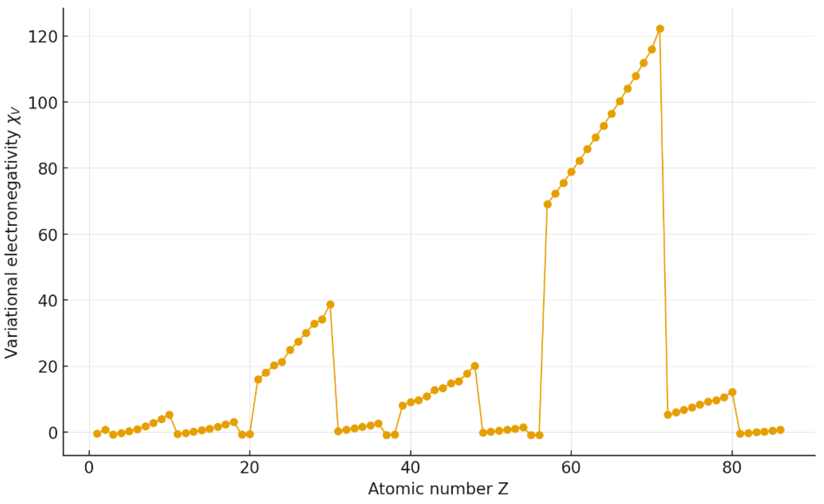
Figure 2.
Linear correlation between Pauling electronegativity () and variational electronegativity (). Regression equation: y = 0.6681 x + 1.6253 (r = 0.948, R² = 0.900).
Figure 2.
Linear correlation between Pauling electronegativity () and variational electronegativity (). Regression equation: y = 0.6681 x + 1.6253 (r = 0.948, R² = 0.900).
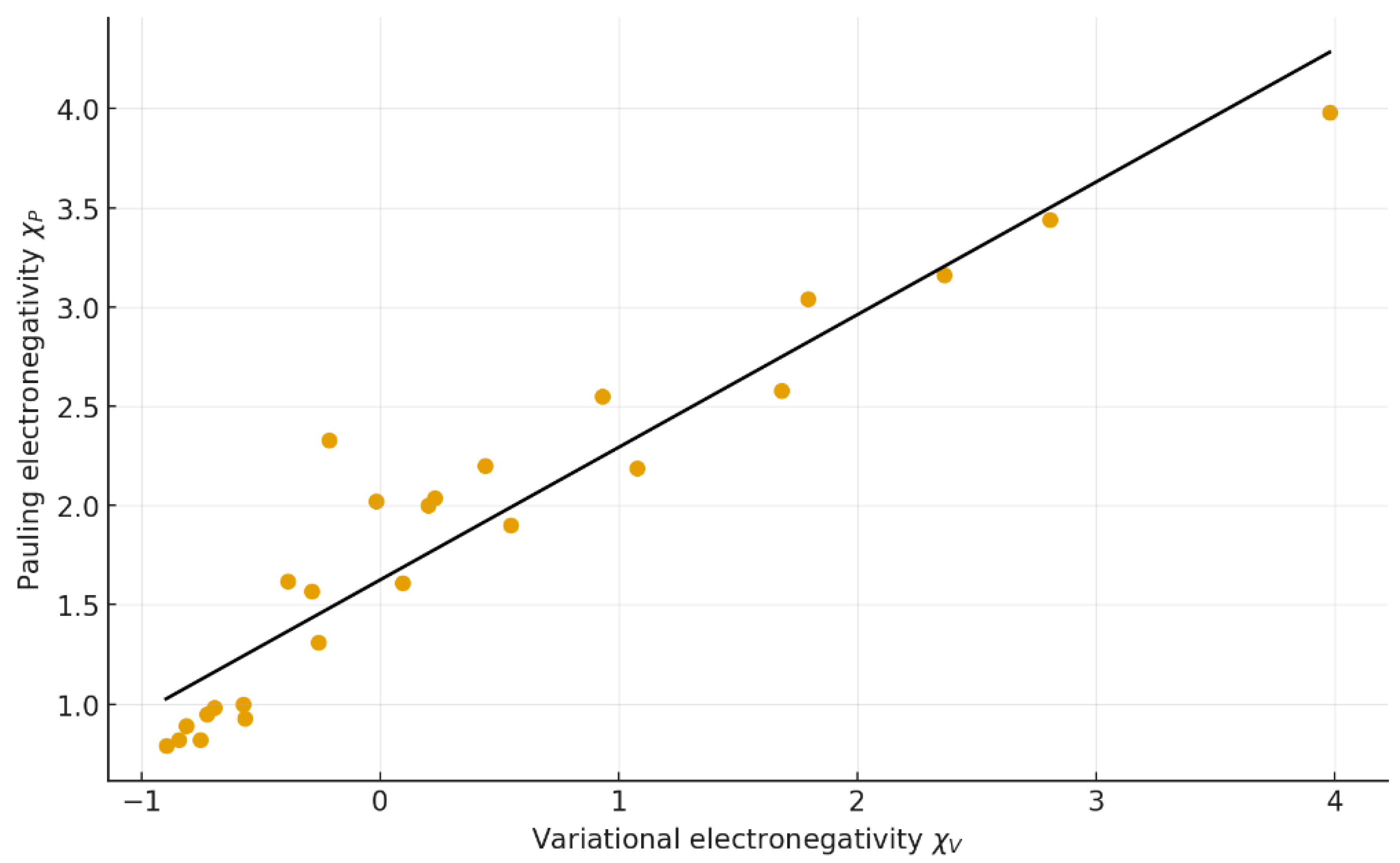
Figure 9.
Periodic surface map of across the elements. The continuous gradient from electropositive to electronegative regions mirrors the patterns of ionization energy and electron affinity, illustrating the unified physical basis of the variational scale.
Figure 9.
Periodic surface map of across the elements. The continuous gradient from electropositive to electronegative regions mirrors the patterns of ionization energy and electron affinity, illustrating the unified physical basis of the variational scale.
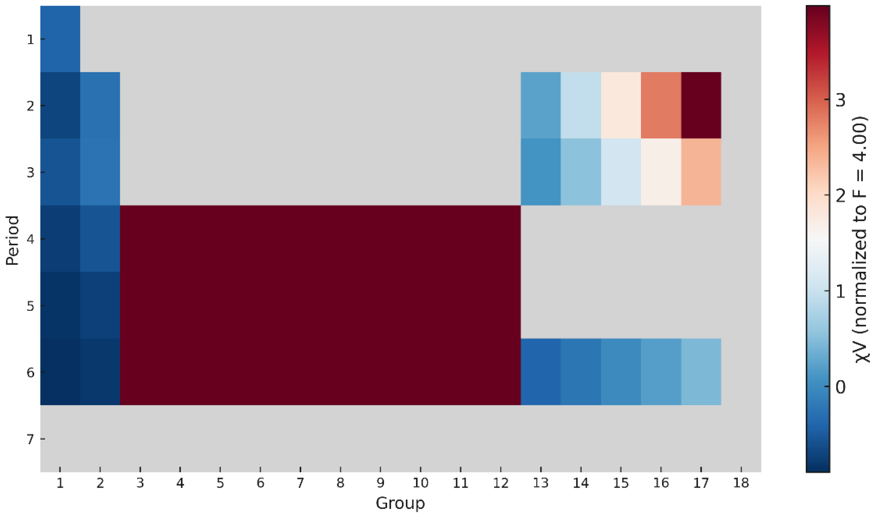
Table 1.
Statistical summary of correlations between , and reference quantities.
| Fig. | Correlation | Regression equation | r | R² | RMSE | MAE | n |
|---|---|---|---|---|---|---|---|
| 2 | χP vs χV | y = 0.668 x + 1.625 | 0.948 | 0.900 | 0.28 | 0.23 | 25 |
| 3 | Ei vs χV | y = 13.320 x + 13.606 | 1.000 | 1.000 | 0.10 | 0.09 | 25 |
| 5 | χM vs χV | y = 7.008 x + 6.952 | 0.969 | 0.939 | 0.95 | 0.73 | 25 |
| 6 | χAR vs χV | y = 0.829 x + 0.411 | 0.913 | 0.834 | 1.40 | 1.04 | 25 |
| 7 | χV vs 1/r² | y = 9.561 x¹·⁰⁸⁸ | 0.951 | 0.904 | 0.26 | 0.19 | 65 |
Disclaimer/Publisher’s Note: The statements, opinions and data contained in all publications are solely those of the individual author(s) and contributor(s) and not of MDPI and/or the editor(s). MDPI and/or the editor(s) disclaim responsibility for any injury to people or property resulting from any ideas, methods, instructions or products referred to in the content. |
© 2025 by the authors. Licensee MDPI, Basel, Switzerland. This article is an open access article distributed under the terms and conditions of the Creative Commons Attribution (CC BY) license (http://creativecommons.org/licenses/by/4.0/).
Copyright: This open access article is published under a Creative Commons CC BY 4.0 license, which permit the free download, distribution, and reuse, provided that the author and preprint are cited in any reuse.


