
Submitted:
31 January 2025
Posted:
03 February 2025
You are already at the latest version
Abstract
This study introduces a fragmentation-based linear-scaling method for strongly correlated systems, specifically the divide-and-conquer Hartree-–Fock-–Bogoliubov (DC-HFB) approach. Two energy gradient formulations of the DC-HFB method are derived and implemented, enabling efficient optimization of molecular geometries in large systems. This method is applied to graphene nanoribbons (GNRs) to explore their geometries and polyradical characters. Numerical results demonstrate that the present DC-HFB method has a potential to treat the static electron correlation and predict diradical character in GNRs, offering new avenues for studying large-scale strongly correlated systems.
Keywords:
quantum chemistry
; electronic structure theory
; electron correlation
; large system
; static correlation
; diradical
1. Introduction
A simple yet accurate description of the static electron correlation, especially in large systems, is still a challenging problem in the electronic structure theory. The static electron correlation is often closely related to the chemical structure. For example, the bond-alternating polyene chain has a weaker static correlation than the chain with a uniform bond length. The transition-state structures often suffer from stronger static correlation than the stable structures. Polyacenes [1] and graphene nanoribbons (GNRs) [2] exhibit different strengths of static correlation depending on their size, shape, and topology (sheet, moebius, or twisted) [3]. In these systems, the strength of the static correlation is related to the diradical character [4]. The diradical character was originally defined in the context of the valence configuration interaction wavefunction [5]. The definition based on the natural orbital occupation numbers obtained from the unrestricted Hartree–Fock (UHF) density matrix was also proposed [6,7]. In particular, Nakano has conducted detailed research into the relationship between the diradical character and excited state properties such as the optical response [8,9,10].
The standard method for describing the static electron correlation is the active-space self-consistent field (SCF) method, typified by the complete active-space SCF (CASSCF) method [11]. These methods require the specification of the active space that defines the strongly correlated orbitals and electrons. Although the recent advent of the density matrix renormalization group method [12,13,14,15] allows much larger active space to be handled than before, its application is still limited to medium-sized systems.
Another way to account for the static correlation is based on the two-electron wavefunction, called geminal [16,17,18]. These schemes, including generalized valence bond methods [19]. only treat two opposite-spin electrons in the variational way, and the other dynamical correlation may be incorporated in the perturbational manner [20,21]. Although the formal computational scaling for these methods can be lower than the CASSCF method with large active space, the simultaneous optimization of orbitals and CI coefficients usually causes serious convergence problems. Note that the geminal method is also related to the pair coupled cluster theories [22,23].
An alternative approach to static correlation problems inspired by the geminal-based method is the Hartree–Fock–Bogoliubov (HFB) method reformulated for quantum chemical problems [24]. Since the HFB wavefunction is related to the antisymmetrized geminal power wavefunction by the particle-number projection [25], the HFB method can effectively describe the static electron correlation, although the obtained as-is HFB wavefunction is contaminated by the different particle-number wavefunctions. The formal computational scaling for the HFB method is similar to that of the Hartree–Fock (HF) method with doubled basis functions. However, we have proposed a method to apply the linear-scaling divide-and-conquer (DC) scheme [26,27,28] to the HFB method [29].
To predict molecular geometry from the quantum chemical calculations, energy gradient must be formulated and implemented in the computational code [30]. One of the authors (MK) has formulated the HFB energy gradient [31]. Note that Chai and coworkers have proposed thermally-assisted occupation density functional theory (TAO-DFT) [32,33,34]. This method can consider the static electron correlation by introducing fictitious electronic temperature and its energy gradient is available. On the other hand, in the DC method, the energy gradient was proposed in the earliest Yang and Lee paper in HF and DFT frameworks [26]. Since this DC energy gradient expression includes an approximation, MK and coworkers delived the exact DC-HF/DFT energy gradient and proposed an improved approximate energy gradient expression [35].
In this paper, we derived two energy gradient expressions for the DC-HFB method in accordance with Refs. [YangDM-DC,KKASNDC-SCFgrad]. The accuracy of these two gradient expressions is investigated in calculations of GNRs including polyacenes. In addition, the strength of the static electron correlation is discussed from the natural orbitals of the HFB wavefunction and their occupation numbers, which are closely related to the diradical, tetraradical, and hexaradical characters. Although the simultaneous consideration of the dynamical electron correlation as well as the static correlation is necessary for the quantitative discussion, we focus here only on the static correlation for the basic evaluation of the method. The organization of this paper is the following. The theoretical perspective of the present method is given in Section 2. The numerical assessment in calculations of GNRs are presented in Section 3. Finally, Section 4 gives the concluding remarks.
2. Theory
2.1. Restricted DC-HFB Method
We here focus on the restricted HFB method for simplicity [31]. Through this paper, Greek-letter indices refer to the basis functions [i.e., atomic orbitals (AOs) that can be non-orthogonal] and refer to the quasiparticle orbitals with negative eigenvalues. The restricted HFB energy can be expressed as the functional of the density matrix and the paring matrix :
where , is the one-electron integral matrix, represents the overlap matrix of the non-orthogonal basis functions, and is a scaling factor introduced by Staroverov and Scuseria [24]. is the chemical potential that is tuned to keep the number of electrons in the system to be . The density and pairing matrices constitute the generalized density matrix :
Variation of the energy (1) with respect to the generalized density matrix (2) leads to the restricted HFB Hamiltonian
where is the shifted Fock matrix,
with , and is the pairing-field matrix,
The eigenvectors of the HFB Hamiltonian (3), ,
represent the quasiparticle orbitals with negative eigenvalues (), which are connected to the density and pairing matrices as follows:
Here, M represents the number of quasiparticle orbitals. Note that the generalized density matrix of the converged HFB solution is idempotent, namely,
In the DC method, the entire system is spatially divided into disjoint subsystems called the central region, where the set of AOs in subsystem is denoted by and the union of becomes the set of basis functions over the entire system denoted by as follows:
When constructing MOs for subsystem , the AOs of atoms adjacent to the central region, called the buffer region denoted by , are taken into consideration in addition to . The union of the central and buffer regions of subsystem is called the localization region, in which the set of AOs is denoted by :
In the DC-HFB method [29], the generalized density matrix of Equation (2) is approximated as sum of subsystem contributions:
where is the partition matrix defined by
Using the submatrices of and for , denoted by and , subsystem density and pairing matrices are obtained with the subsystem quasiparticle orbitals obtained as the eigenvectors of the following subsystem HFB equation
as
with the number of quasiparticle orbitals in subysystem , . Another expression that is consistent to the DC-HF method with the finite electronic temperature of is the following:
where is the Fermi distribution function. Note that the summation over p runs all the quasiparticle orbitals regardless of the sign of the eigenvalues.
2.2. DC-HFB Energy Gradient with Respect to Atomic Coordinate
According to Ref. [KHFBgrad], the differentiation of Equation (1) with respect to atomic coordinate Q gives
The first term, , represents the Hellmann–Feynman (H–F) force that relates to the derivatives of the Hamiltonian matrix elements, and the second term is the so-called Pulay force. In case of the variational solution, the evaluation of and derivatives with respect to Q can be avoided by using the idempotency condition of the generalized density matrix, , as [31]
where is the energy-weighted density matrix defined by
Note that the eigenvalues of Equation (6) are .
As similar to the DC-HF energy gradient [35], the Pulay force of the DC-HFB energy gradient cannot be simplified to the form of Equation (23) because the DC-HFB density and pairing matrices are not variationally determined. However, as Yang and Lee [26] proposed, the Pulay force can be approximated in the similar manner to the DC density and pairing matrices of Equations (14) and (15) as
Therefore, the DC-HFB energy gradient can be approximated as the following:
According to Ref. [KKASNDC-SCFgrad], this formula is referred to as the YL formula throughout this paper.
Alternatively, the Pulay force in the DC-HFB energy can be reformulated as the following:
On the analogy to the formulation in Ref. [KKASNDC-SCFgrad], we here assume that the subsystem generalized density matrix,
also satisfies the idempotency condition, leading
Furthermore, we regard that the subsystem generalized density matrices, , are variationally determined. Then, any simultaneous solution of the derivatives of Equations (30) and (31),
gives the same force [36]. A simple set of solutions is the following [31]:
Applying Equations (34) and (35) to the Pulay force of Equation (28) and considering the subsystem HFB equation of Equation (17) leads to
where is the subsystem energy-weighted pairing matrix defined by
Finally, the following approximated DC-HFB energy gradient can be obtained:
where
3. Numerical Application to Graphene Nanoribbons
Single-layer graphene sheet shows characteristic electronic properties such as fractional quantum Hall effect [37] and ultrafast carrier mobility [38] due to its special band structure derived from the electronic structure confined in a plane. Graphene-based spintronics devices are also expected to be developed, [38,39] although the band gap has to be generated for realizing these devices. GNRs were theoretically expected to generate band gap [40,41] and have also been experimentally reported. Since the electronic properties of GNRs depend on the geometrical factors such as width, length, and edge shape, it is essential to understand their relation with the electronic structure in order to design GNR-based nanodevices. To obtain the correct electronic structures of GNRs, known as strongly correlated systems, high-level ab initio multireference methods such as the density matrix renormalization group (DMRG) [4,42] and the second-order reduced density matrix-based variational method [43] are required. However, due to their large computational demands, their applications to larger GNRs are difficult. In addition, at the current stage, the geometry optimization based on these high-level ab initio methods is not tructable.
Here, we performed the geometry optimizations of GNRs with the DC-HFB energy gradient and investigated the polyradical character of GNRs from the HFB natural orbital occupation. After a (DC-)HFB calculation, the natural orbitals can be obtained by diagonalizing the density matrix, . The eigenvalues correspond to the natural orbital occupation numbers (NOONs), which has been discussed as the indicator of diradical character in UHF calculations [44]. For single-reference systems, NOON is either 0 (unoccupied) or 2 (two-electron occupied), while for singlet diradical systems with electrons, the highest occupied (i.e., -th) and lowest unoccupied (i.e., -th) natural orbitals (HONO and LUNO) are degenerate, resulting in NOON being 1 [45]. Throughout this paper, the modified version of the Gamess program package [46,47] was used for computations of the standard and DC-HFB energy and gradient.
3.1. Determination of Parameter
Before applying the HFB method to GNRs, the scaling factor, , has to be fixed. Here, this parameter was determined by comparing the optimized geometries of phenalenyl cation, anthracene, and phenanthrene (Figure 1) with those by reference all- CASSCF calculations, which were performed with the OpenMolcas 24.10 program [48]. No dynamical correlation correction was introduced to the CASSCF reference since the HFB method basically cannot account for the dynamical correlation. Throughout this paper, the 6-31G** basis set [49,50] was adopted. The obtained CASSCF geometries for phenalenyl cation, anthracene, and phenanthrene have the , , and symmetries, respectively, the stabilities of which are confirmed by the frequency analysis.
Table 1 and Table 2 summarize the optimized C–C and C–H bond lengths, respectively, for these molecules obtained with CASSCF and HFB methods. For HFB calculations, the parameter is varied between 0.75 and 1.0. The mean absolute deviations (MADs) of the HFB results from the CASSCF reference results are also listed. The deviations of the C–C bond lengths are one-order (or more) larger than those of the C–H lengths. The HFB results with include obviously larger deviation than the others. For both the C–C and C–H lengths, the HFB results with gives the smallest MADs from the CASSCF ones. Hereafter, was adopted.
3.2. Polyradicality of Graphene Nanoribbons
The HFB calculations were performed for GNRs of different widths (W) and lengths (L) to investigate the effect of edge structure on polyradicality. The width W and length L are defined as shown in Figure 2. For this sample molecule, we denote . NOONs for (HONO) to (LUNO) were examined as a measure of polyradicality. The geometries were also optimized at the HFB/6-31G** level of theory.
First, we fixed the width and varied the zigzag edge length . NOONs for six frontier natural orbitals are summarized in Figure 3. The occupation number difference between HONO and LUNO rapidly decreases as L increases, indicating that the diradical character of the system is increasing along L. In addition, the differences between (HONO)/(HONO) and (LUNO)/(LUNO) also decreases gradually, indicating the increase of tetra- and hexa-radical characters in these systems.
Next, we fixed the length and varied the armchair edge width , of which the results are depicted in Figure 4. Again, the occupation number difference between HONO and LUNO decreases as W increases, but the rate of decrease is slower than the result in Figure 3. The reason can be deduced from the shapes of HONO and LUNO. The HONOs and LUNOs of the GNRs with and are illustrated in Figure 5 and Figure 6, respectively. Since the occupation numbers for these NOs are , the electron distribution represented by these NOs corresponds to the distribution of the singlet diradical. It can be confirmed that the radical electrons are mainly localized on zigzag edges. Therefore, diradical character is enhanced when the zigzag edge is elongated than when the armchair edge is elongated.
Figure 7 (a) shows the HONO-LUNO occupation number difference of GNRs plotted against the number of carbon atoms. For the same number of carbon atoms, the series, in which the zigzag edge increases with the smallest armchair edge fraction, has the highest diradical character. Conversely, the series, in which the armchair edge increases with the smallest zigzag edge fraction, has the lowest diradical character. The difference in the occupation numbers between HONO and LUNO, which is an indicator of tetraradicality, is shown in Figure 7 (b), and a similar trend is seen especially in W-constant series. In the L-constant series, if the number of carbon atoms is taken as the horizontal axis, the and series are reversed in the middle. This is probably due to the fact that radicals tend to localize at the armchair edge compared to the center of the GNR.
3.3. DC-HFB Optimization of GNR Structures
In this subsection, the geometry optimization of the GNR with was performed by the standard and DC-HFB method. In the DC-HFB calculations, two different gradient formalisms, namely KKASN and YL formulas, as well as two different fragmentation schemes, namely type A and B as shown in Figure 8 were investigated.
First the fragmentation scheme was set to type A. Figure 9 shows the optimized C–C bond lengths at the zigzag edge with respect to the sequential position. In the DC calculations, up to -th nearest fragments were included in the buffer region. Although alternating single and double bond structure can be found around the end points, the bond alternation rapidly decreases around the center. For DC with , the structure obtained with the YL formula significantly differs from the standard one. The difference significantly diminishes when adopting KKASN formula. The mean absolute deviations (MADs) from the standard HFB result are Å and Å for YL and KKASN formulas, respectively. As the buffer size increases to , the structure deviation decreases by about one order of magnitude both for KKASN and YL formulas. The MADs are Å and Å, respectively.
Figure 10 shows the energy convergence process in the geometry optimization of GNR with . The initial structure was set with the uniform bond lengths and angles, namely, Å, Å, and 120 for C–C bond lengths, C–H bond lengths, and bond angles, respectively. For the DC-HFB results with , the energy convergence process is almost equivalent to the standard HFB one. The deviations of the energy at the optimized structure are and for KKASN and YL formulas, respectively. At first glance, the YL formula seems to produce better result than the KKASN one, but the energy difference between the DC and standard HFB results for the initial structure is , so this is due to the error cancellation caused by the slightly poorer structure by the YL formula. For the combination of smaller buffer size of and the YL formula, the energy gradually increased from the third iteration and converged to higher energy structure after more than 20 iterations. However, when combined with the KKASN formula, the energy converged as smoothly as the case, while the energy is lower than the standard HFB result.
Finally, the dependence on the fragmentation scheme was investigated. Figure 11 shows the optimized C–C bond lengths at the zigzag edge with respect to the sequential position. The type A results are equivalent to those given in Figure 9. Especially for the small buffer size of , the trend is different between different fragmentation schemes, namely, the type A fragmentation emphasizes the bond alternation than the type B one. However, for the large buffer size of , the geometry is almost identical. For the type B fragmentation, the MADs from the standard HFB result are Å and Å for and 4, respectively, which are slightly smaller than for the type A fragmentation.
4. Concluding Remarks
This study presented the divide-and-conquer Hartree–-Fock-–Bogoliubov (DC-HFB) method as an effective approach for the treatment of static electron correlation in large molecular systems. The analysis of natural orbitals obtained from the HFB denstiy matrix revealed that GNRs exhibit strong polyradical character, particularly in structures with extended zigzag edges, which is consistent with previous computational reports. The proposed two approximate energy gradient formulations, specifically the YL and KKASN methods, demonstrated their utility in the geometry optimization of graphene nanoribbons (GNRs). In general, the KKASN method gives more accurate gradient and geometry than the YL one. These results highlight the DC-HFB method’s scalability and accuracy for large-scale systems, making it a promising tool for quantum chemical calculations in strongly correlated systems. As mentioned in the introduction, incorporating dynamical electron correlation is required to further enhance the quantitative accuracy of the method. A simple scheme to incorporate dynamical electron correlation is to combine the HFB method with the Kohn-Sham density functional theory (DFT), which has already been accomplished by Tsuchimochi et al. [51]. Its DC-based linear-scaling implementation as well as its energy gradient formulation will be straightforward, since the DC method was originally proposed in DFT.
Recently, we have proposed a time-dependent (TD) HFB method for the excited-state calculation of molecular systems [52]. Since the real-time propagation scheme is adopted in this excited-state calculation method, the DC-TD-HFB formulation will be possible, opening up the excited-state calculation of large-scale statically correlated systems. In addition, the HFB wavefunction (and of course the DC-HFB method) suffers from the contamination of the different particle number wavefunctions, which is related to the spin contamination in the UHF wavefunction. The projected HFB or UHF method, which extracts the desired particle-number or spin states, respectively, from the contaminated wavefunction, has been proposed [25,53]. The application of the DC scheme to these projected HF theories is currently underway and will be presented in the near future.
Author Contributions
Conceptualization, M.K.; methodology, M.K., R.K., and T.A.; software, M.K. and R.K.; investigation, M.K.; writing—original draft preparation, M.K.; writing—review and editing, M.K., T.A., and T.T.; project administration, M.K.; funding acquisition, M.K. All authors have read and agreed to the published version of the manuscript.
Funding
This research was funded by JSPS KAKENHI Grant Numbers JP25810011, JP15H00908, JP17K05738, and JP23H04093, by MEXT as “Program for Promoting Research on the Supercomputer Fugaku” Grant Number JPMXP1020230325.
Acknowledgments
Some of the present calculations were performed using the computer facilities at Research Center for Computational Science, Okazaki (Project: 24-IMS-C017), and at Research Institute for Information Technology, Kyushu University, Japan. The Institute for Chemical Reaction Design and Discovery (ICReDD) was established by the World Premier International Research Initiative (WPI), MEXT, Japan.
Conflicts of Interest
The authors declare no conflicts of interest.
References
- Houk, K.N.; Lee, P.S.; Nendel, M. Polyacene and Cyclacene Geometries and Electronic Structures: Bond Equalization, Vanishing Band Gaps, and Triplet Ground States Contrast with Polyacetylene. The Journal of Organic Chemistry 2001, 66, 5517–5521. [Google Scholar] [CrossRef] [PubMed]
- Tian, C.; Miao, W.; Zhao, L.; Wang, J. Graphene nanoribbons: Current status and challenges as quasi-one-dimensional nanomaterials. Reviews in Physics 2023, 10, 100082. [Google Scholar] [CrossRef]
- Caetano, E.W.S.; Freire, V.N.; dos Santos, S.G.; Galvão, D.S.; Sato, F. Möbius and twisted graphene nanoribbons: Stability, geometry, and electronic properties. The Journal of Chemical Physics 2008, 128. [Google Scholar] [CrossRef] [PubMed]
- Mizukami, W.; Kurashige, Y.; Yanai, T. More π Electrons Make a Difference: Emergence of Many Radicals on Graphene Nanoribbons Studied by Ab Initio DMRG Theory. Journal of Chemical Theory and Computation 2012, 9, 401–407. [Google Scholar] [CrossRef]
- Hayes, E.F.; Siu, A.K.Q. Electronic structure of the open forms of three-membered rings. Journal of the American Chemical Society 1971, 93, 2090–2091. [Google Scholar] [CrossRef]
- Head-Gordon, M. Characterizing unpaired electrons from the one-particle density matrix. Chemical Physics Letters 2003, 372, 508–511. [Google Scholar] [CrossRef]
- Nakano, M.; Fukui, H.; Minami, T.; Yoneda, K.; Shigeta, Y.; Kishi, R.; Champagne, B.; Botek, E.; Kubo, T.; Ohta, K.; et al. (Hyper)polarizability density analysis for open-shell molecular systems based on natural orbitals and occupation numbers. Theoretical Chemistry Accounts 2011, 130, 711–724. [Google Scholar] [CrossRef]
- Nakano, M. Excitation Energies and Properties of Open-Shell Singlet Molecules: Applications to a New Class of Molecules for Nonlinear Optics and Singlet Fission; Springer International Publishing, 2014. [CrossRef]
- Nakano, M. Open-Shell-Character-Based Molecular Design Principles: Applications to Nonlinear Optics and Singlet Fission. The Chemical Record 2016, 17, 27–62. [Google Scholar] [CrossRef]
- Nakano, M.; Champagne, B. Nonlinear optical properties in open-shell molecular systems. WIREs Computational Molecular Science 2016, 6, 198–210. [Google Scholar] [CrossRef]
- Roos, B.O. The Complete Active Space Self-Consistent Field Method and its Applications in Electronic Structure Calculations; Wiley Blackwell (John Wiley & Sons), 1987; pp. 399–445. [CrossRef]
- Zgid, D.; Nooijen, M. The density matrix renormalization group self-consistent field method: Orbital optimization with the density matrix renormalization group method in the active space. The Journal of Chemical Physics 2008, 128. [Google Scholar] [CrossRef]
- Nakatani, N.; Guo, S. Density matrix renormalization group (DMRG) method as a common tool for large active-space CASSCF/CASPT2 calculations. The Journal of Chemical Physics 2017, 146. [Google Scholar] [CrossRef]
- Olivares-Amaya, R.; Hu, W.; Nakatani, N.; Sharma, S.; Yang, J.; Chan, G.K.L. The ab-initio density matrix renormalization group in practice. The Journal of Chemical Physics 2015, 142. [Google Scholar] [CrossRef] [PubMed]
- Baiardi, A.; Reiher, M. The density matrix renormalization group in chemistry and molecular physics: Recent developments and new challenges. The Journal of Chemical Physics 2020, 152. [Google Scholar] [CrossRef] [PubMed]
- Surján, P.R. An Introduction to the Theory of Geminals. In Correlation and Localization; Surján, P.R., Ed.; Springer: Berlin, 1999. [Google Scholar] [CrossRef]
- Limacher, P.A.; Ayers, P.W.; Johnson, P.A.; De Baerdemacker, S.; Van Neck, D.; Bultinck, P. A New Mean-Field Method Suitable for Strongly Correlated Electrons: Computationally Facile Antisymmetric Products of Nonorthogonal Geminals. J. Chem. Theory Comput. 2013, 9, 1394–1401. [Google Scholar] [CrossRef]
- Tarumi, M.; Kobayashi, M.; Nakai, H. Accelerating convergence in the antisymmetric product of strongly orthogonal geminals method. Int. J. Quantum Chem. 2013, 113, 239–244. [Google Scholar] [CrossRef]
- Bobrowicz, F.W.; Goddard, W.A. The Self-Consistent Field Equations for Generalized Valence Bond and Open-Shell Hartree—Fock Wave Functions. In Methods of Electronic Structure Theory; Springer US, 1977; pp. 79–127. [CrossRef]
- Kobayashi, M.; Szabados, Á.; Nakai, H.; Surján, P.R. Generalized Møller-Plesset Partitioning in Multiconfiguration Perturbation Theory. J. Chem. Theory Comput. 2010, 6, 2024–2033. [Google Scholar] [CrossRef]
- Tarumi, M.; Kobayashi, M.; Nakai, H. Generalized Møller-Plesset Multiconfiguration Perturbation Theory Applied to an Open-Shell Antisymmetric Product of Strongly Orthogonal Geminals Reference Wave Function. J. Chem. Theory Comput. 2012, 8, 4330–4335. [Google Scholar] [CrossRef]
- Henderson, T.M.; Bulik, I.W.; Scuseria, G.E. Pair extended coupled cluster doubles. The Journal of Chemical Physics 2015, 142. [Google Scholar] [CrossRef]
- Lehtola, S.; Head-Gordon, M. Coupled-cluster pairing models for radicals with strong correlations, 2025. [CrossRef]
- Staroverov, V.N.; Scuseria, G.E. Optimization of density matrix functionals by the Hartree-Fock-Bogoliubov method. J. Chem. Phys. 2002, 117, 11107–11112. [Google Scholar] [CrossRef]
- Scuseria, G.E.; Jiménez-Hoyos, C.A.; Henderson, T.M.; Samanta, K.; Ellis, J.K. Projected quasiparticle theory for molecular electronic structure. J. Chem. Phys. 2011, 135, 124108. [Google Scholar] [CrossRef]
- Yang, W.; Lee, T.S. A density-matrix divide-and-conquer approach for electronic structure calculations of large molecules. J. Chem. Phys. 1995, 103, 5674–5678. [Google Scholar] [CrossRef]
- Nakai, H.; Kobayashi, M.; Yoshikawa, T.; Seino, J.; Ikabata, Y.; Nishimura, Y. Divide-and-Conquer Linear-Scaling Quantum Chemical Computations. The Journal of Physical Chemistry A 2023, 127, 589–618. [Google Scholar] [CrossRef]
- Kobayashi, M.; Nakai, H. Papadopoulos, M.G., Zalesny, R., Mezey, P.G., Leszczynski, J., Eds.; Divide-and-conquer approaches to quantum chemistry: Theory and implementation. In Linear-Scaling Techniques in Computational Chemistry and Physics: Methods and Applications; Springer: Dordrecht, 2011. [Google Scholar] [CrossRef]
- Kobayashi, M.; Taketsugu, T. Divide-and-Conquer Hartree-Focko-Bogoliubov Method and Its Application to Conjugated Diradical Systems. Chem. Lett. 2016, 45, 1268–1270. [Google Scholar] [CrossRef]
- Pulay, P. Analytical derivatives, forces, force constants, molecular geometries, and related response properties in electronic structure theory. WIREs Computational Molecular Science 2014, 4, 169–181. [Google Scholar] [CrossRef]
- Kobayashi, M. Gradient of molecular Hartree–Fock–Bogoliubov energy with a linear combination of atomic orbital quasiparticle wave functions. The Journal of Chemical Physics 2014, 140, 084115. [Google Scholar] [CrossRef]
- Chai, J.D. Density functional theory with fractional orbital occupations. J. Chem. Phys. 2012, 136, 154104. [Google Scholar] [CrossRef]
- Wu, C.S.; Chai, J.D. Electronic Properties of Zigzag Graphene Nanoribbons Studied by TAO-DFT. J. Chem. Theory Comput. 2015, 11, 2003–2011. [Google Scholar] [CrossRef]
- Chen, B.J.; Chai, J.D. TAO-DFT fictitious temperature made simple. RSC Advances 2022, 12, 12193–12210. [Google Scholar] [CrossRef]
- Kobayashi, M.; Kunisada, T.; Akama, T.; Sakura, D.; Nakai, H. Reconsidering an analytical gradient expression within a divide-and-conquer self-consistent field approach: Exact formula and its approximate treatment. J. Chem. Phys. 2011, 134, 034105. [Google Scholar] [CrossRef]
- Pulay, P. Ab initio calculation of force constants and equilibrium geometries in polyatomic molecules. I. Theory. Mol. Phys. 1969, 17, 197–204. [Google Scholar] [CrossRef]
- Bolotin, K.I.; Ghahari, F.; Shulman, M.D.; Stormer, H.L.; Kim, P. Observation of the fractional quantum Hall effect in graphene. Nature 2009, 462, 196–199. [Google Scholar] [CrossRef] [PubMed]
- Novoselov, K.S.; Geim, A.K.; Morozov, S.V.; Jiang, D.; Katsnelson, M.I.; Grigorieva, I.V.; Dubonos, S.V.; Firsov, A.A. Two-dimensional gas of massless Dirac fermions in graphene. Nature 2005, 438, 197–200. [Google Scholar] [CrossRef] [PubMed]
- Zhang, Y.; Tan, Y.W.; Stormer, H.L.; Kim, P. Experimental observation of the quantum Hall effect and Berry’s phase in graphene. Nature 2005, 438, 201–204. [Google Scholar] [CrossRef] [PubMed]
- Son, Y.W.; Cohen, M.L.; Louie, S.G. Energy Gaps in Graphene Nanoribbons. Physical Review Letters 2006, 97. [Google Scholar] [CrossRef]
- Barone, V.; Hod, O.; Scuseria, G.E. Electronic Structure and Stability of Semiconducting Graphene Nanoribbons. Nano Letters 2006, 6, 2748–2754. [Google Scholar] [CrossRef]
- Hachmann, J.; Dorando, J.J.; Avilés, M.; Chan, G.K.L. The radical character of the acenes: A density matrix renormalization group study. The Journal of Chemical Physics 2007, 127, 134309. [Google Scholar] [CrossRef]
- Pelzer, K.; Greenman, L.; Gidofalvi, G.; Mazziotti, D.A. Strong Correlation in Acene Sheets from the Active-Space Variational Two-Electron Reduced Density Matrix Method: Effects of Symmetry and Size. The Journal of Physical Chemistry A 2011, 115, 5632–5640. [Google Scholar] [CrossRef]
- Pulay, P.; Hamilton, T.P. UHF natural orbitals for defining and starting MC-SCF calculations. The Journal of Chemical Physics 1988, 88, 4926–4933. [Google Scholar] [CrossRef]
- Mizukami, W.; Kurashige, Y.; Yanai, T. More π Electrons Make a Difference: Emergence of Many Radicals on Graphene Nanoribbons Studied by Ab Initio DMRG Theory. Journal of Chemical Theory and Computation 2012, 9, 401–407. [Google Scholar] [CrossRef]
- Schmidt, M.W.; Baldridge, K.K.; Boatz, J.A.; Elbert, S.T.; Gordon, M.S.; Jensen, J.H.; Koseki, S.; Matsunaga, N.; Nguyen, K.A.; Su, S.; et al. General atomic and molecular electronic structure system. J. Comput. Chem. 1993, 14, 1347–1363. [Google Scholar] [CrossRef]
- Gordon, M.S.; Schmidt, M.W. Advances in electronic structure theory: GAMESS a decade later. In Theory and Applications of Computational Chemistry: the first forty years; Dykstra, C.E., Frenking, G., Kim, K.S., Scuseria, G.E., Eds.; Elsevier: Amsterdam, 2005. [Google Scholar]
- Li Manni, G.; Fdez. Galván, I.; Alavi, A.; Aleotti, F.; Aquilante, F.; Autschbach, J.; Avagliano, D.; Baiardi, A.; Bao, J.J.; Battaglia, S.; et al. The OpenMolcas Web: A Community-Driven Approach to Advancing Computational Chemistry. Journal of Chemical Theory and Computation 2023, 19, 6933–6991. [Google Scholar] [CrossRef] [PubMed]
- Hehre, W.J.; Ditchfield, R.; Pople, J.A. Self-consistent molecular orbital methods. XII. Further extensions of Gaussian-type basis sets for use in molecular orbital studies of organic molecules. J. Chem. Phys. 1972, 56, 2257. [Google Scholar] [CrossRef]
- Hariharan, P.C.; Pople, J.A. The influence of polarization functions on molecular orbital hydrogenation energies. Theor. Chim. Acta 1973, 28, 213–222. [Google Scholar] [CrossRef]
- Tsuchimochi, T.; Scuseria, G.E.; Savin, A. Constrained-pairing mean-field theory. III. Inclusion of density functional exchange and correlation effects via alternative densities. J. Chem. Phys. 2010, 132, 024111. [Google Scholar] [CrossRef]
- Nishida, M.; Akama, T.; Kobayashi, M.; Taketsugu, T. Time-dependent Hartree–Fock–Bogoliubov method for molecular systems: An alternative excited-state methodology including static electron correlation. Chemical Physics Letters 2023, 816, 140386. [Google Scholar] [CrossRef]
- Jiménez-Hoyos, C.A.; Henderson, T.M.; Tsuchimochi, T.; Scuseria, G.E. Projected Hartree–Fock theory. The Journal of Chemical Physics 2012, 136. [Google Scholar] [CrossRef]
Figure 1.
Structures of phenalenyl cation, anthracene, and phenanthrene.
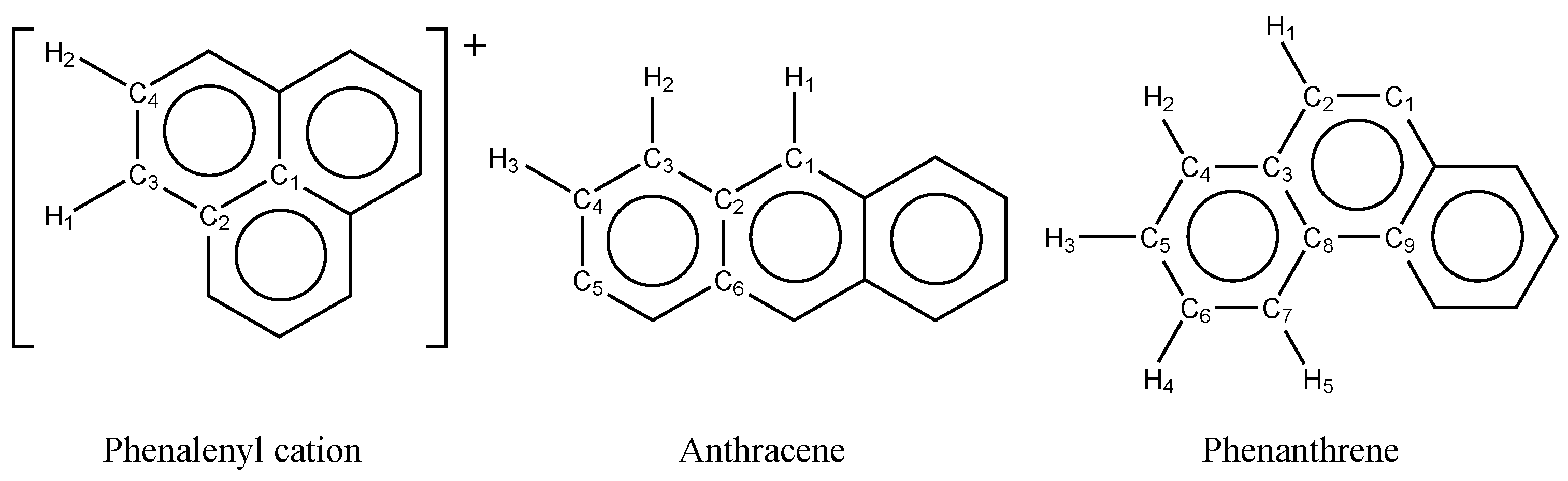
Figure 2.
Structure of GNRs and definitions of length L and width W.
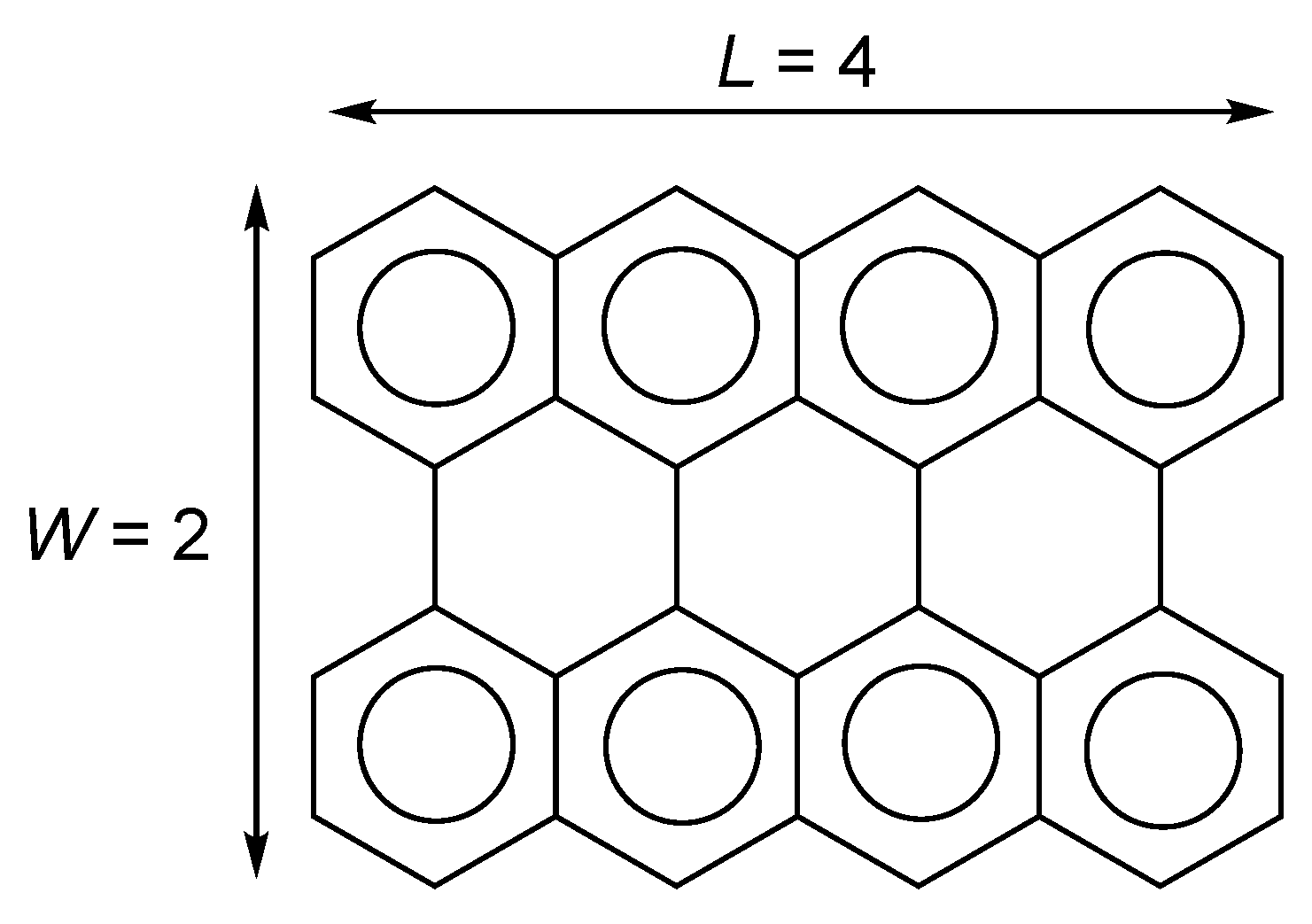
Figure 3.
NOONs for (HONO) to (LUNO) of GNRs with .
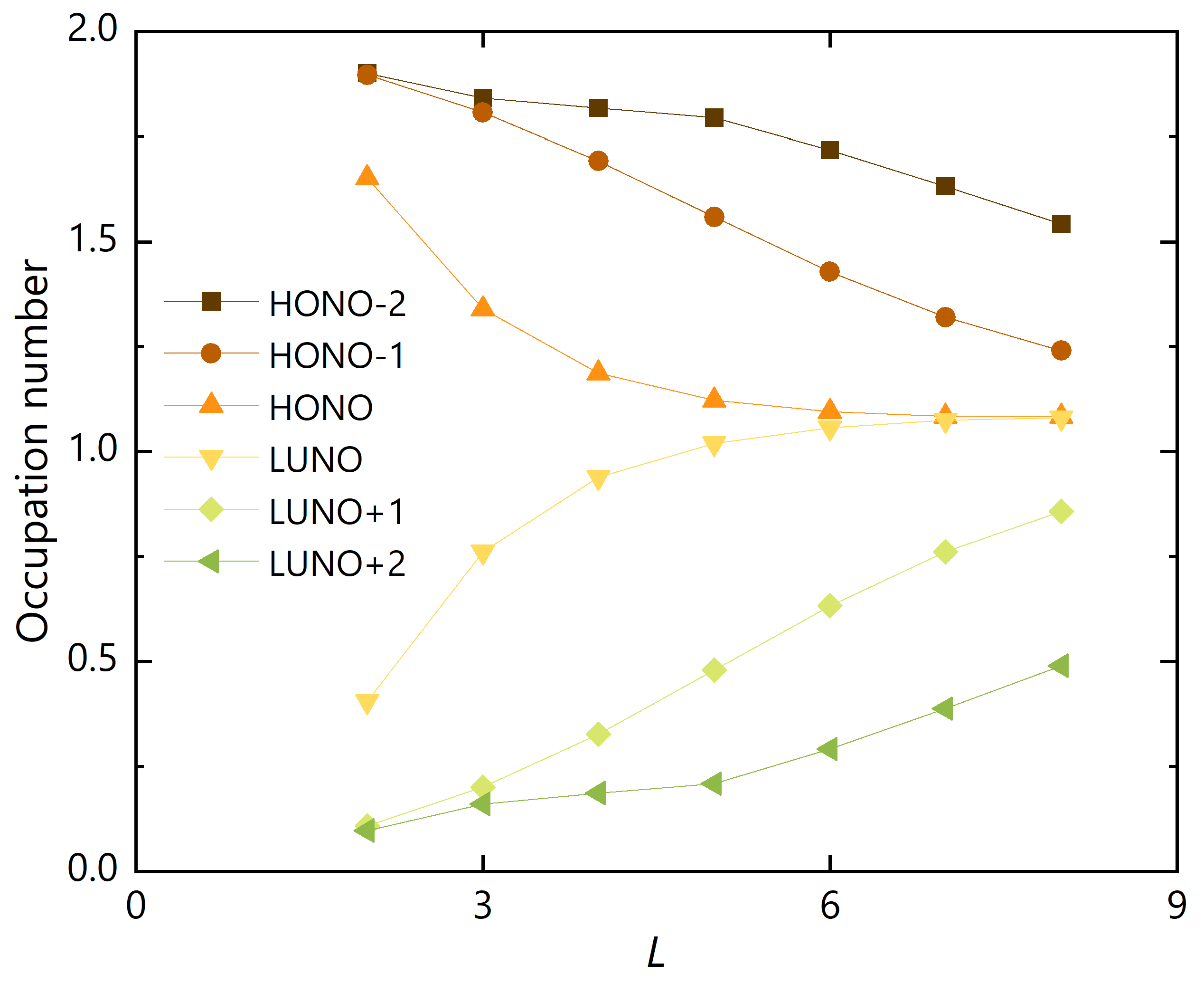
Figure 4.
NOONs for (HONO) to (LUNO) of GNRs with .
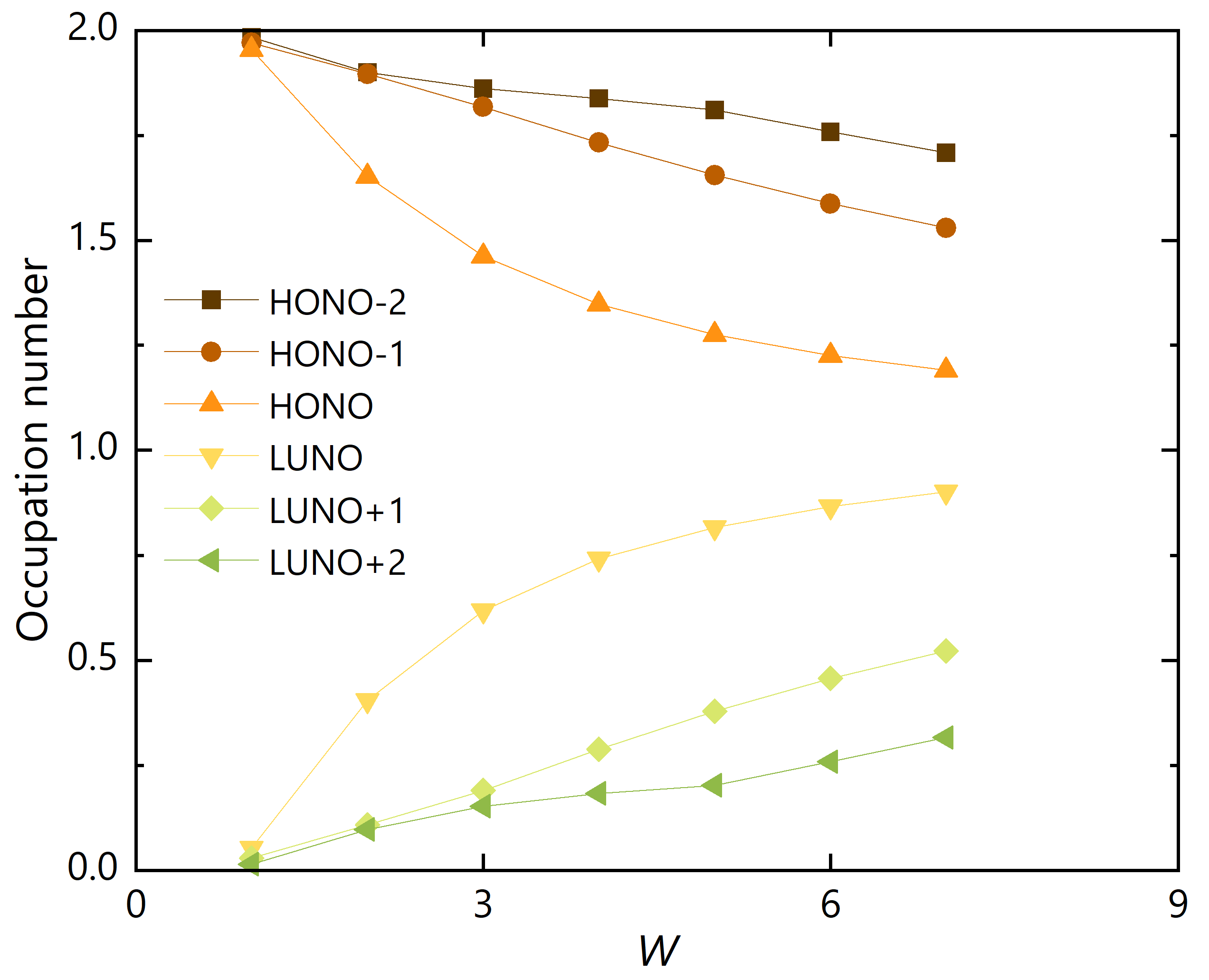
Figure 5.
(a) HONO and (b) LUNO obtained from the HFB calculation of GNR with . The value in parentheses is the occupation number.
Figure 5.
(a) HONO and (b) LUNO obtained from the HFB calculation of GNR with . The value in parentheses is the occupation number.
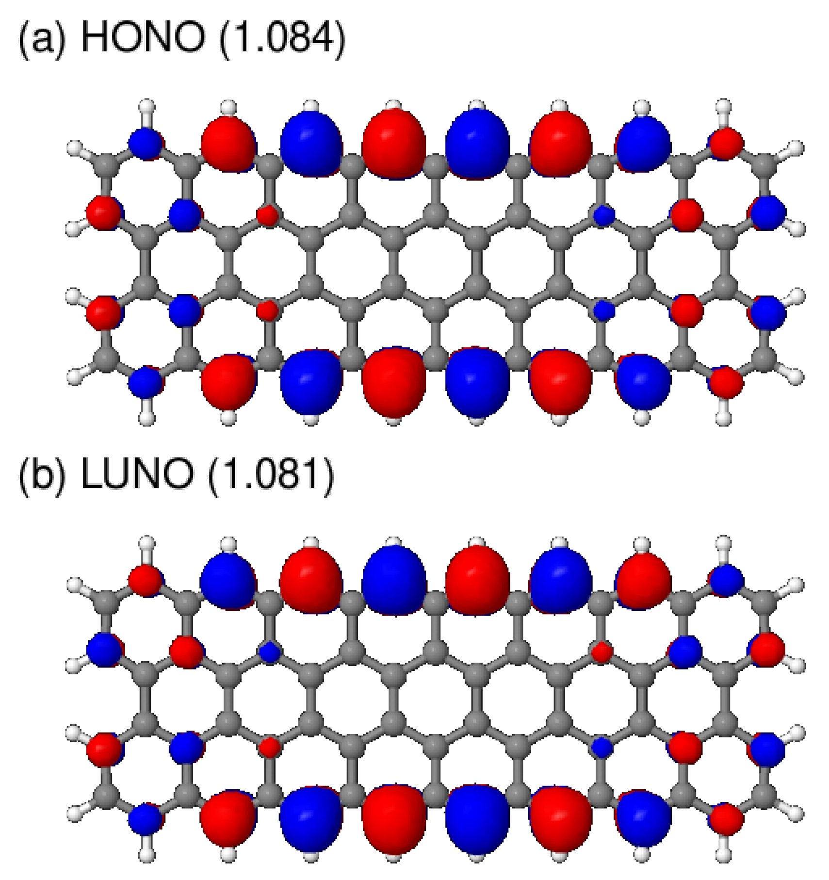
Figure 6.
(a) HONO and (b) LUNO obtained from the HFB calculation of GNR with . The value in parentheses is the occupation number.
Figure 6.
(a) HONO and (b) LUNO obtained from the HFB calculation of GNR with . The value in parentheses is the occupation number.
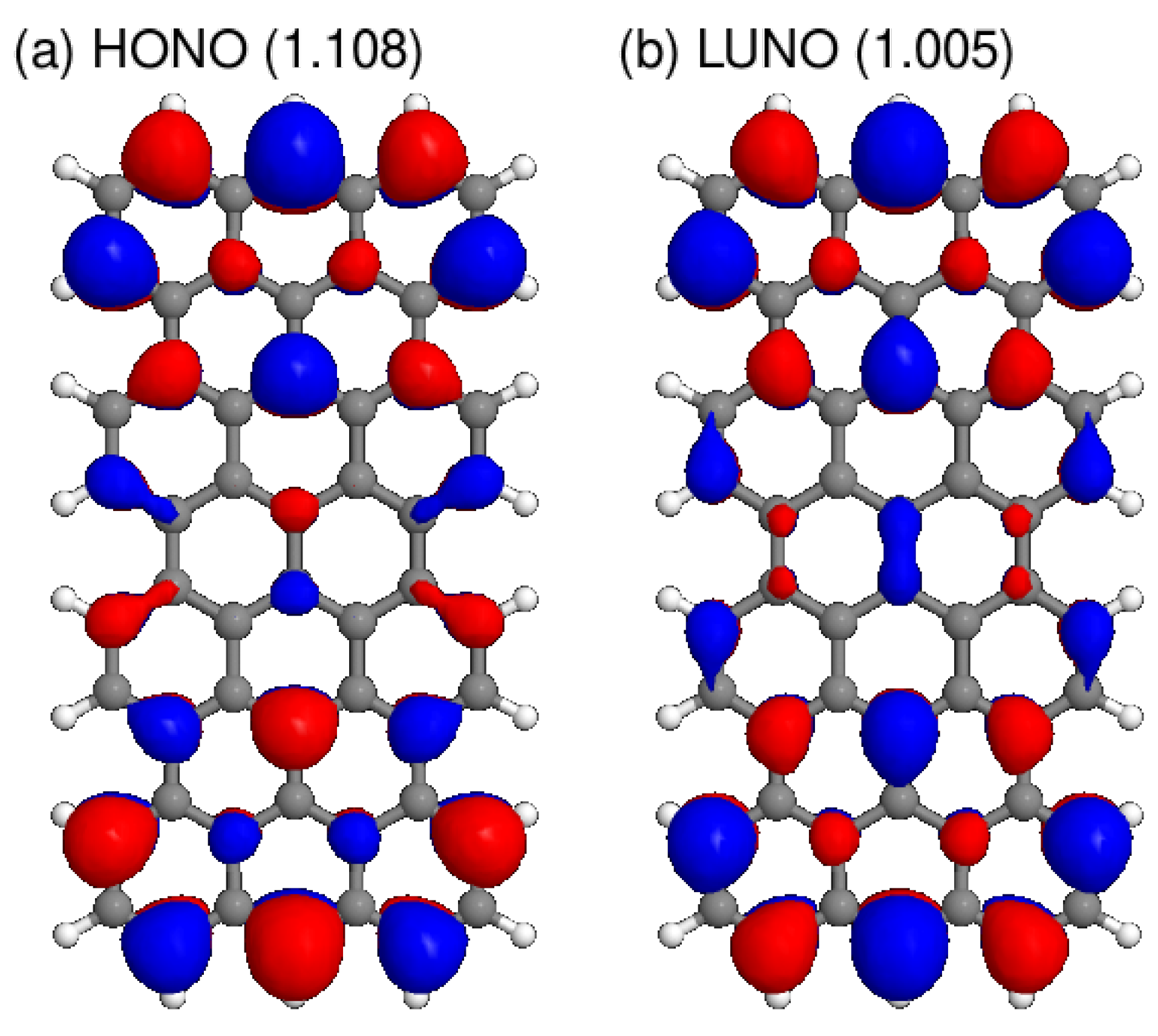
Figure 7.
Occupation number differences of GNRs between (a) HONO and LUNO and (b) (HONO) and (LUNO) against the number of carbon atoms, .
Figure 7.
Occupation number differences of GNRs between (a) HONO and LUNO and (b) (HONO) and (LUNO) against the number of carbon atoms, .
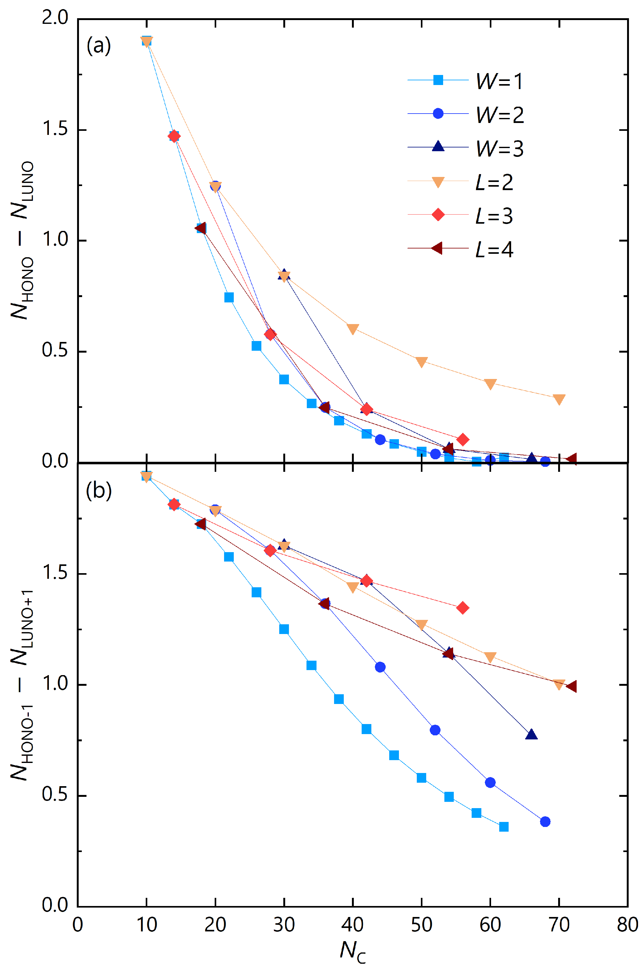
Figure 8.
Two fragmentation schemes adopted in the DC-HFB calculations of GNR with .
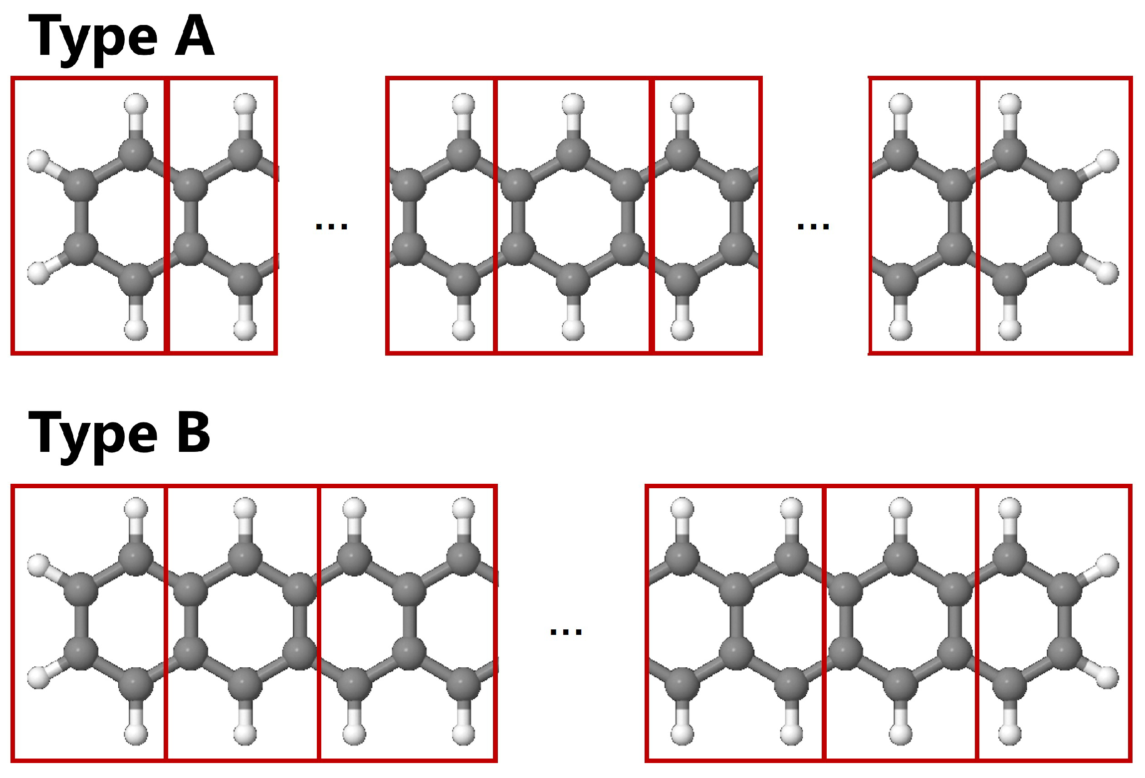
Figure 9.
C–C bond lengths of GNR with optimized with DC and standard HFB methods.
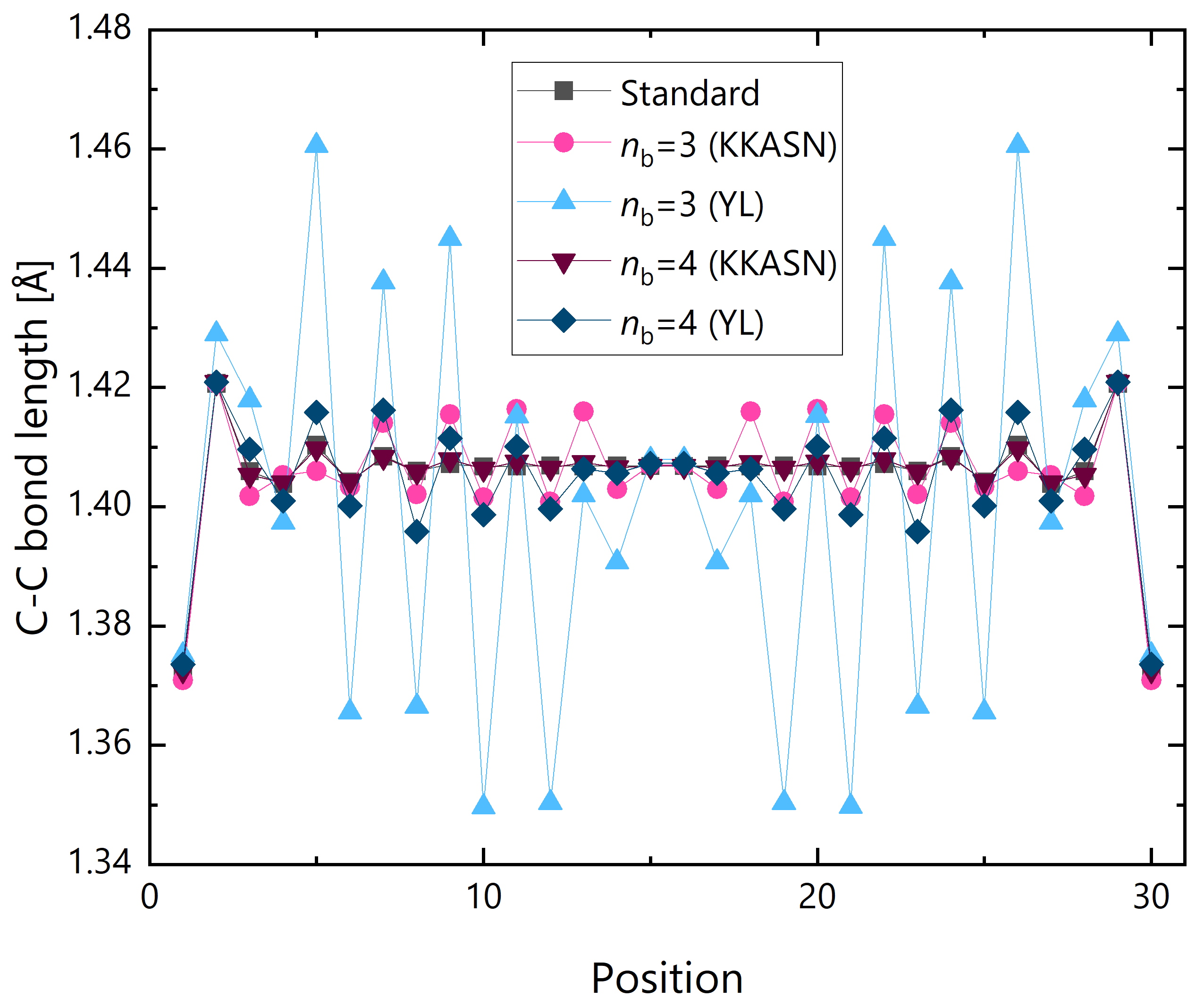
Figure 10.
Energy convergence process in the geometry optimization of GNR with in DC and standard HFB calculations.
Figure 10.
Energy convergence process in the geometry optimization of GNR with in DC and standard HFB calculations.
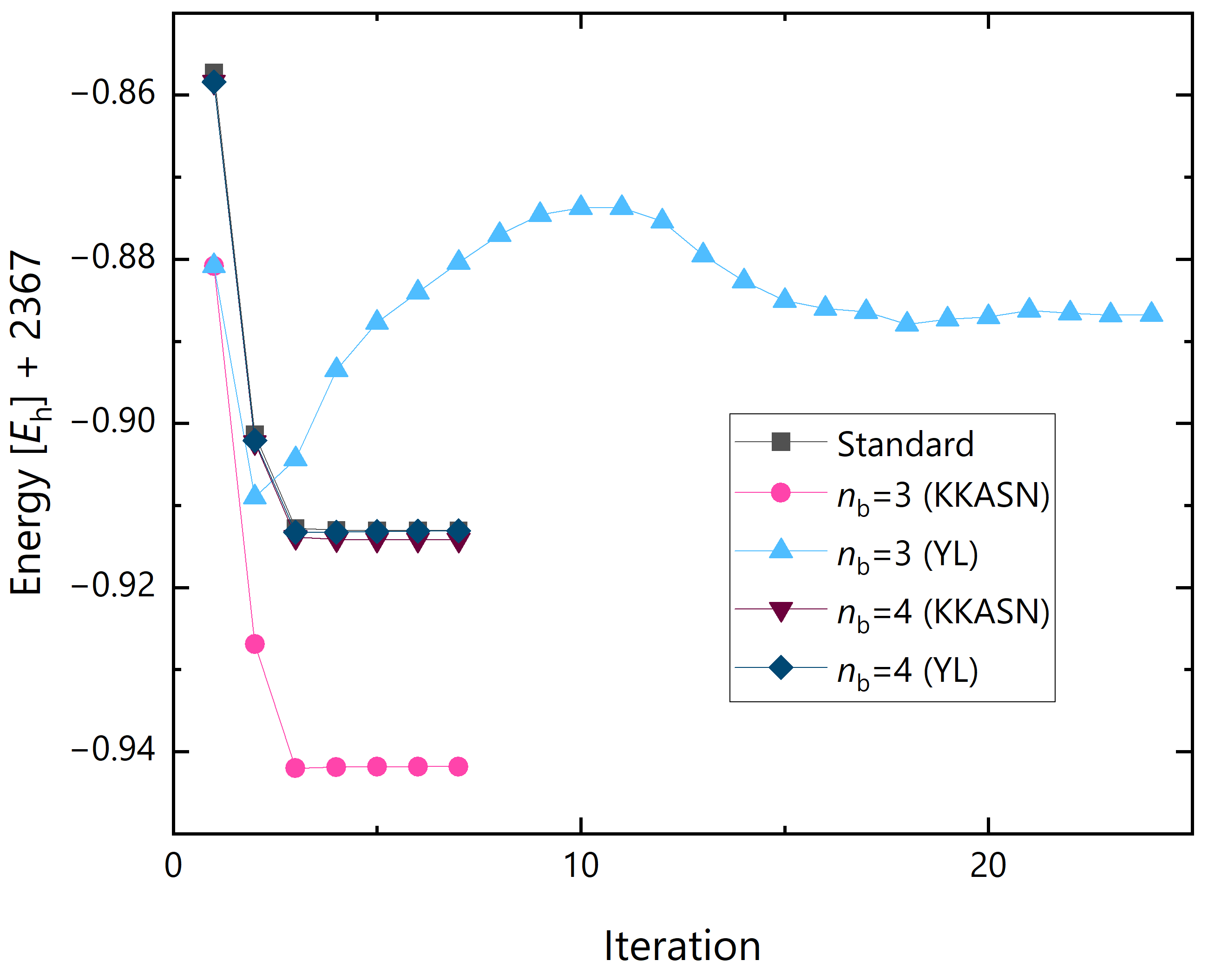
Figure 11.
xxx GNR with .
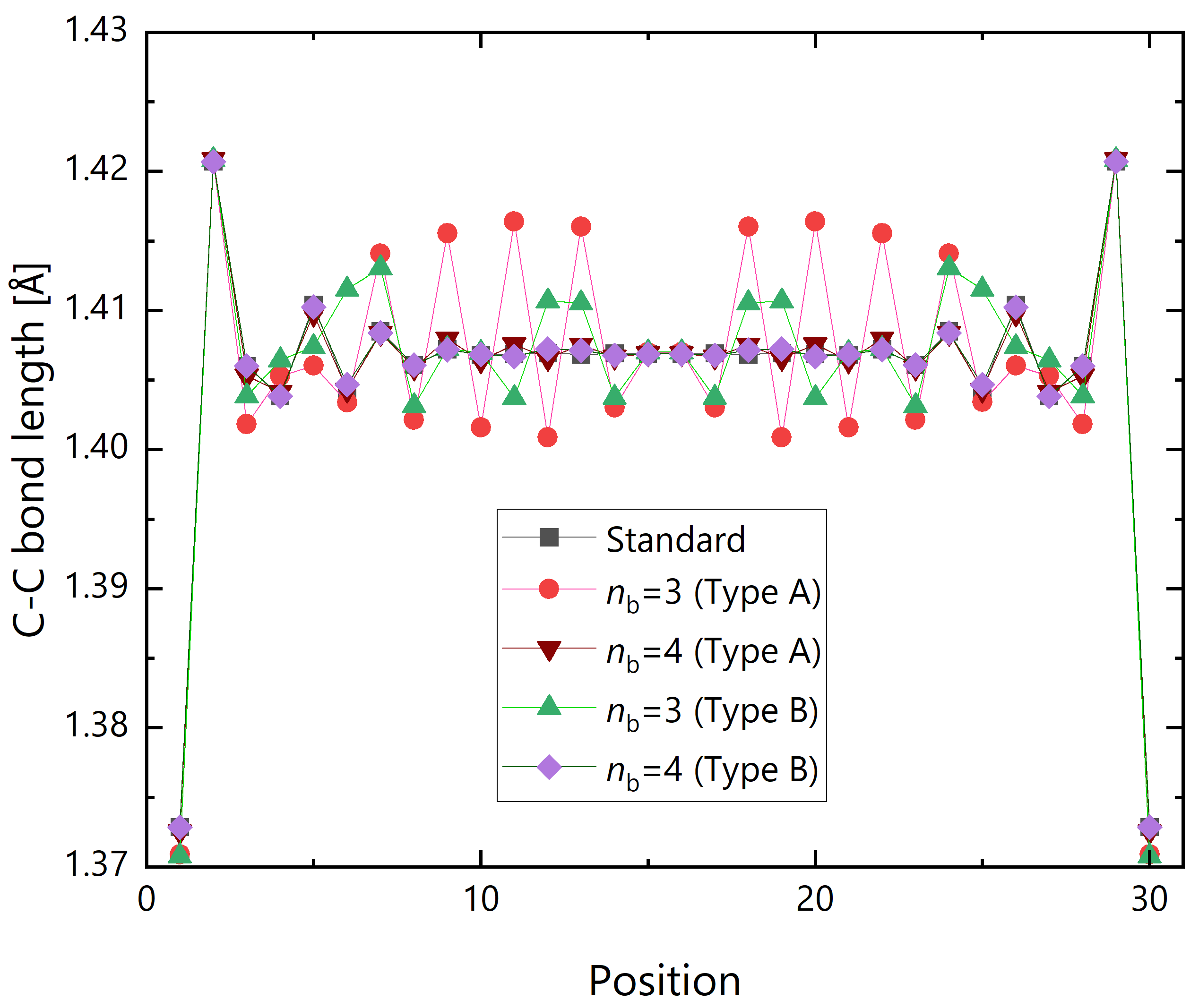

Table 1.
Optimized C–C bond lengths (in Å) of phenalenyl cation, anthracene, and phenanthrene obtained with CASSCF and HFB methods.
Table 1.
Optimized C–C bond lengths (in Å) of phenalenyl cation, anthracene, and phenanthrene obtained with CASSCF and HFB methods.
| HFB | |||||||
| Molecule | Position | CASSCF | |||||
| Phenalenyl cation | C1–C2 | 1.4178 | 1.4107 | 1.4164 | 1.4228 | 1.4297 | 1.4487 |
| C2–C3 | 1.4141 | 1.4087 | 1.4121 | 1.4157 | 1.4198 | 1.4344 | |
| C3–C4 | 1.3921 | 1.3834 | 1.3873 | 1.3921 | 1.3982 | 1.4173 | |
| Anthracene | C1–C2 | 1.4008 | 1.3894 | 1.3893 | 1.4009 | 1.4106 | 1.4299 |
| C2–C3 | 1.4385 | 1.4359 | 1.4359 | 1.4252 | 1.4218 | 1.4343 | |
| C3–C4 | 1.3649 | 1.3473 | 1.3473 | 1.3671 | 1.3863 | 1.4156 | |
| C4–C5 | 1.4337 | 1.4324 | 1.4325 | 1.4183 | 1.4114 | 1.4213 | |
| C2–C6 | 1.4287 | 1.4246 | 1.4245 | 1.4330 | 1.4409 | 1.4557 | |
| Phenanthrene | C1–C2 | 1.3557 | 1.3386 | 1.3386 | 1.3479 | 1.3730 | 1.4080 |
| C2–C3 | 1.4424 | 1.4405 | 1.4405 | 1.4356 | 1.4269 | 1.4329 | |
| C3–C4 | 1.4166 | 1.4084 | 1.4084 | 1.4100 | 1.4163 | 1.4341 | |
| C4–C5 | 1.3780 | 1.3656 | 1.3656 | 1.3707 | 1.3856 | 1.4134 | |
| C5–C6 | 1.4090 | 1.4017 | 1.4017 | 1.4022 | 1.4048 | 1.4188 | |
| C6–C7 | 1.3802 | 1.3677 | 1.3677 | 1.3730 | 1.3886 | 1.4165 | |
| C3–C8 | 1.4127 | 1.4043 | 1.4043 | 1.4127 | 1.4324 | 1.4570 | |
| C7–C8 | 1.4192 | 1.4106 | 1.4106 | 1.4119 | 1.4177 | 1.4370 | |
| C8–C9 | 1.4634 | 1.4612 | 1.4612 | 1.4576 | 1.4520 | 1.4589 | |
| MAD | 0.0080 | 0.0073 | 0.0057 | 0.0113 | 0.0251 | ||
Table 2.
Optimized C–H bond lengths (in Å) of phenalenyl cation, anthracene, and phenanthrene obtained with CASSCF and HFB methods.
Table 2.
Optimized C–H bond lengths (in Å) of phenalenyl cation, anthracene, and phenanthrene obtained with CASSCF and HFB methods.
| HFB | |||||||
| Molecule | Position | CASSCF | |||||
| Phenalenyl cation | C3–H1 | 1.0752 | 1.0758 | 1.0753 | 1.0752 | 1.0755 | 1.0791 |
| C4–H2 | 1.0734 | 1.0731 | 1.0736 | 1.0741 | 1.0747 | 1.0784 | |
| Anthracene | C1–H1 | 1.0769 | 1.0768 | 1.0768 | 1.0768 | 1.0773 | 1.0818 |
| C3–H2 | 1.0763 | 1.0762 | 1.0762 | 1.0763 | 1.0767 | 1.0806 | |
| C4–H3 | 1.0756 | 1.0756 | 1.0756 | 1.0757 | 1.0760 | 1.0796 | |
| Phenanthrene | C2–H1 | 1.0761 | 1.0761 | 1.0761 | 1.0761 | 1.0765 | 1.0806 |
| C4–H2 | 1.0763 | 1.0763 | 1.0763 | 1.0763 | 1.0767 | 1.0806 | |
| C5–H3 | 1.0755 | 1.0755 | 1.0755 | 1.0755 | 1.0759 | 1.0794 | |
| C6–H4 | 1.0756 | 1.0757 | 1.0757 | 1.0757 | 1.0760 | 1.0797 | |
| C7–H5 | 1.0727 | 1.0727 | 1.0727 | 1.0728 | 1.0732 | 1.0776 | |
| MAD | 0.0001 | 0.0001 | 0.0001 | 0.0005 | 0.0044 | ||
Disclaimer/Publisher’s Note: The statements, opinions and data contained in all publications are solely those of the individual author(s) and contributor(s) and not of MDPI and/or the editor(s). MDPI and/or the editor(s) disclaim responsibility for any injury to people or property resulting from any ideas, methods, instructions or products referred to in the content. |
© 2025 by the authors. Licensee MDPI, Basel, Switzerland. This article is an open access article distributed under the terms and conditions of the Creative Commons Attribution (CC BY) license (http://creativecommons.org/licenses/by/4.0/).
Copyright: This open access article is published under a Creative Commons CC BY 4.0 license, which permit the free download, distribution, and reuse, provided that the author and preprint are cited in any reuse.


