Submitted:
06 February 2026
Posted:
09 February 2026
You are already at the latest version
Abstract
In this paper, we propose a metaheuristic optimization algorithm called Adaptive Gold Rush Optimizer (AGRO), a substantial evolution of the original Gold Rush Optimizer (GRO). Unlike the standard GRO, which relies on fixed probabilities in the strategy selection process, AGRO utilizes a novel adaptive mechanism that prioritizes strategies improving solution quality. This adaptive component, that can be applied to any optimization algorithm with fixed probabilities in the strategy selection, adjusts the probabilities of the three core search strategies of GRO (Migration, Collaboration, and Panning), in real-time, rewarding those that successfully improve solution quality. Furthermore, AGRO introduces fundamental modifications to the search equations, eliminating the inherent attraction towards the zero coordinates, while explicitly incorporating objective function values to guide prospectors towards promising regions. Experimental results demonstrate that AGRO outperforms ten state-of-the-art algorithms on the twenty-three classical benchmark functions, the CEC2017, and the CEC2019 datasets. The source code of AGRO algorithm is publicly available at https://sites.google.com/site/costaspanagiotakis/research/agro.
Keywords:
gold rush optimizer
; metaheuristic
; artificial intelligence
; global optimization
; benchmark function
; swarm intelligence
; population-based algorithm
1. Introduction
The goal of optimization is to search for the global optimal value (minimum or maximum). The algorithms used for this search process are called optimization algorithms, which are broadly classified into deterministic methods and metaheuristic algorithms [1].
Deterministic algorithms are capable of locating the exact global optimum for small-scale and simple problems but face significant limitations. These approaches are prone to stagnation in local optima, often require gradient information of the objective functions, and can be computationally expensive [2]. However, as modern scientific and engineering challenges evolve, there is an increasing need to solve large-scale and high-dimensional optimization problems [3]. Due to the complexity, non-linearity, and high dimensionality of these real-world problems, traditional deterministic algorithms often fail to locate the global optimum efficiently. To address these challenges, nature-inspired metaheuristic algorithms have been proposed. Although there were about 150 metaheuristic algorithms before 2012, their number rapidly increased to 540 by 2022 [4], with an almost linear growth rate, indicating that efficient global optimum estimation remains an open problem that attracts significant research interest. In recent decades, seminal metaheuristic algorithms such as Particle Swarm Optimization (PSO) [5], Gravitational Search Algorithm (GSA) [6], Grey Wolf Optimizer (GWO) [7], Whale Optimization Algorithm (WOA) [8] and Weighted Mean of Vectors [9] have demonstrated remarkable success in solving complex optimization tasks.
Metaheuristic optimization algorithms search for the optimal solution via a method called “trial and error” and are classified into single-based and population-based algorithms [9,10]. The search process for single-based algorithms begins with a single solution and updates its position during the optimization process, e.g., simulated annealing [11] and tabu search [12]. These algorithms are typically straightforward to implement and computationally inexpensive. However, their main drawback is the high probability of convergence to local optima. This limitation is addressed by population-based algorithms, in which the optimization process starts from a set of candidate solutions whose positions are iteratively updated during the search.
Most of metaheuristic algorithms search for the optimal solution using exploration and exploitation phases after randomly initializing population and obtaining the first optimal solution [13,14]. During the exploration phase, the algorithm navigates the search space globally to identify promising regions. In contrast, the exploitation phase focuses on refining the search locally within these identified areas to locate the precise optimum. Excessive exploration can lead to insufficient exploitation, which will lead to low accuracy of the search solution, while over-exploitation can cause the candidate solution to fall into local optima. The balance between these two phases is a challenging issue for any optimization algorithm, since no precise rule has been established to distinguish the most appropriate time to transit from exploration to exploitation due to the unexplored form of search spaces. Figure 1 presents a graphical illustration of the task of locating the highest peak by employing both exploration and exploitation strategies. Exploration is characterized by discovering new regions using large steps, and exploitation, focusing on refining the highest peak using small steps.
The foundation of modern metaheuristics was laid by classical evolutionary and physics-based algorithms. Pioneers in the field include Genetic Algorithms (GA) [15,16], which simulate Darwinian natural selection, and Simulated Annealing (SA) [17], inspired by the physical process of slowly cooling metals. Alongside these, Differential Evolution (DE) [18] emerged as a powerful tool for global optimization. Building on these foundations, Swarm Intelligence was introduced with Particle Swarm Optimization (PSO) [5], mimicking the social behavior of bird flocks, Ant Colony Optimization (ACO) [19,20], mimicking the social behavior of ants, and Gravitational Search Algorithm (GSA) [6], based on the laws of gravity and mass interactions.
Subsequently, numerous bio-inspired approaches have been introduced in the literature, many of which are based on imitating animal hunting behaviors, including the Grey Wolf Optimizer (GWO) [7,21] inspired by the hierarchy and hunting of wolves, the Whale Optimization Algorithm (WOA) [8], which models the bubble-net feeding of humpback whales, the Harris Hawks Optimization (HHO) [22] based on the cooperative hunting behavior and social intelligence of Harris’s hawks, and the Snake Optimizer (SO) [23] which mimics the foraging and mating behaviors of snakes. More recently, algorithms like the FOX Optimizer [24] and the Blood-sucking Leech Optimizer (BLSO) [13] have been introduced, simulating the foraging behavior of leeches and foxes, respectively.
Beyond animal-inspired methods, researchers have looked to plant life, proposing the Dandelion Optimizer (DO) [25], based on the wind-driven dissemination of dandelion seeds, and the Sequoia Optimization Algorithm (SOA) [26], inspired by the self-regulating dynamics and resilience of sequoia forest ecosystems. Furthermore, human behavior has inspired the Political Optimizer (PO) [27], which models the multi-phased process of politics such as constituency allocation, party switching, election campaign, inter-party election, and parliamentary affairs, and the Gold Rush Optimizer (GRO) [10], which mimics gold prospectors. Other approaches like INFO [9] rely purely on mathematical concepts, utilizing weighted vector means and computational geometry.
According to the literature review, the majority of metaheuristic optimization algorithms are typically classified into four categories through various inspirations and evolution mechanisms [13,28]:
- Swarm Intelligence Algorithms inspired by the hunting behavior, hierarchy, and reproductive behavior of plants (e.g., Dandelion Optimizer (DO) [25]), and animals among which are Particle Swarm Optimization (PSO) [5], Ant Colony Optimization (ACO) [20], Grey Wolf Optimizer (GWO) [7], Whale Optimization Algorithm (WOA) [8] and Blood-Sucking Leech Optimizer (BLSO) [13].
In this work, we propose a substantial evolution of the original Gold Rush Optimizer (GRO) [10], called Adaptive Gold Rush Optimizer (AGRO). GRO belongs to the Human-Based Algorithms and mimics the behavior of gold prospectors during the gold rush era using three key concepts of gold prospecting: migration, collaboration, and panning. As the method progresses and approaches its maximum number of iterations, the algorithm progressively shifts from the exploration phase to the exploitation phase by adjusting the search spaces of migration, collaboration and panning processes.
GRO demonstrates high performance on optimization problems compared to other state-of-the-art algorithms [10], which is the primary reason for its selection. However, the main motivation for this work lies in its simplicity compared to recent algorithms like BLSO [13] and DO [25]. These methods consist of complex steps with advanced mathematical formulations that are difficult to refine further. In contrast, GRO’s inspiration leads to an intuitive search process divided into three meaningful strategies with simple formulation, providing a solid basis for modifications and improvements.
AGRO introduces fundamental modifications to the search equations, eliminating the inherent attraction towards the zero coordinates, while explicitly incorporating objective function values (fitness) to guide prospectors towards promising regions. Furthermore, unlike the standard GRO, which relies on fixed probabilities in the strategy selection process, AGRO employs a novel dynamic strategy selection mechanism. This adaptive component adjusts the probabilities of the three core search strategies: Migration, Collaboration, and Panning, in real-time, rewarding those that successfully improve solution quality. The proposed method is compared with the state-of-the-art metaheuristic evolutionary algorithms [5,6,7,8,9,10,13,24,25,26] presented in Table 1 in chronological order.
The main contributions of this paper are summarized as follows:
- The proposal of an Adaptive Gold Rush Optimizer (AGRO) that introduces key enhancements to the traditional GRO, a novel adaptive mechanism that prioritizes strategies improving solution quality, that can be applied to any optimization algorithm with fixed probabilities in the strategy selection.
- Additionally, AGRO explicitly incorporates objective function values to guide prospectors to promising regions.
- High performance results of AGRO against ten state-of-the-art algorithms, including GRO, BLSO, INFO, FOX, DO, WOA, GWO, and PSO.
2. Gold Rush Optimizer (GRO)
The Gold Rush Optimizer (GRO) is a population-based metaheuristic algorithm proposed by Zolfi [10], inspired by the historical events of gold prospectors during the Gold Rush era. The algorithm simulates the search for gold deposits through three distinct search strategies: Migration, Collaboration, and Panning (Mining).
Hereafter, we describe the GRO algorithm for solving the minimization problem. Let be the population of N prospectors (search agents) in a d-dimensional space. The position vector of the i-th prospector at iteration t is denoted by . In every iteration t, a prospector randomly selects one of the three strategies to compute a new position . The prospector’s position in the next iteration, indicated by , is updated only if the amount of gold, represented by the value of the objective function , in the new location is better than in the current location . Equation (1) describes this update rule for the minimization problem.
As the method progresses and approaches its maximum number of iterations (T), the algorithm progressively shifts from the exploration phase to the exploitation phase by adjusting the search spaces of migration, collaboration and panning. This adjustment has been modeled by a linear function () and a quadratic function (), as defined below.
where t denotes the iteration step, . Both of them decrease from 2 at the beginning () to at the last iteration (). The exploration ability of the algorithm is high at the beginning due to the spread distribution of the locations of the prospectors. Since prospectors gradually get close to the best gold mine, their distances to each other are reduced, providing a higher exploitation ability. In the algorithm, this is also achieved by the reduction of search spaces over time, controlled by and . Based on and , the d-dimensional vectors and with random values and , , are defined as follows:
where and are random numbers in that follow uniform distribution. The vectors and are used in migration and panning phases, respectively. The range of the vectors determines the size of the phase search space, which decreases with the number of iterations. Figure 2 illustrates the evolution of , and the range of and during the execution of GRO.
2.1. Migration (Global Oriented Search)
This strategy simulates the movement of prospectors towards the most promising gold deposits identified so far. This phase acts as a convergence mechanism, guiding the population towards the neighborhood of a reference point based on the current global best solution , where prospector is given by Equation (6):
To prevent premature convergence and allow local exploration around the optimum, the algorithm introduces a randomized distance vector based on a randomized vector . The mathematical formulation of the migration strategy is defined as follows:
where:
- is the current position of the i-th prospector in the j-th dimension at iteration t.
- is the position of the best solution in the j-th dimension found so far.
- is the position of the reference point in the j-th dimension, that guides the i-th prospector to prevent premature convergence and allow local exploration.
- is a random number in the interval .
- is a random vector that creates a weighted target point, allowing the prospector to explore the region around the destination rather than directly moving to it.
- is a vector that determines the step size of the movement.
- is the proposed position of the i-th prospector in the j-th dimension at iteration t according to the migration phase.
In this model, the term directs the prospector towards the randomized vicinity of the gold mine, rapidly narrowing the search space. Figure 3a illustrates a schematic representation of the migration phase. The blue rectangle represents the phase search space, centered at the reference point, with side length .
2.2. Collaboration (Information Sharing)
In the collaboration phase, the algorithm mimics the social interaction between gold prospectors, who communicate to share information about promising locations. This strategy promotes knowledge exchange within the population, ensuring that the search agents do not act in isolation, but rather benefit from the collective findings of the swarm.
Unlike Migration, which directs prospectors towards the global best, Collaboration introduces a stochastic search direction derived from the relative positions of other prospectors. Specifically, for the i-th prospector, the algorithm randomly selects two other distinct agents from the population, denoted by indices a and b. The mathematical model for this interaction is formulated as:
where:
- and represent the position vectors of two randomly selected prospectors from the population ().
- is the differential vector representing the direction and magnitude of the interaction between the two selected agents.
- is a random number in the interval , acting as a scaling factor for the influence of the collaboration phase.
- is the proposed position of the i-th prospector in the j-th dimension at iteration t according to the collaboration phase.
By utilizing the differential vector , this strategy enhances the diversity of the population. It allows the algorithm to explore search directions that are not necessarily aligned with the current global optimum, thereby reducing the risk of stagnation in local optima and facilitating a broader exploration of the search space. Figure 3b illustrates a schematic representation of the collaboration phase. The blue rectangle corresponds to the phase search space, with bottom-left corner at and side length equal to .
2.3. Panning (Gold Mining)
Panning or Gold Mining corresponds to the exploitation phase, where a prospector carefully searches the immediate vicinity of a promising area to extract gold. During this phase, a prospector randomly selects another prospector and searches within a region determined by the relative positions of the two prospectors. This phase involves smaller, more precise steps to refine the solution. The mathematical formulation is given by:
where is the position of a randomly selected prospector, is the distance vector, and is a scaling coefficient vector that reduces the search radius over time to facilitate convergence. is the proposed position of the i-th prospector in the j-th dimension at iteration t according to the panning phase. Figure 3c illustrates a schematic representation of the panning phase. The blue rectangle corresponds to the phase search space, centered at the and side length equal to .
3. Adaptive Gold Rush Optimizer (AGRO)
In GRO, the algorithm simulates the search for gold deposits through three distinct search strategies: Migration, Collaboration, and Panning. Adaptive Gold Rush Optimizer (AGRO) addresses the following three issues of GRO to further improve its performance.
- Strategy Adaptation: In each iteration of GRO, the prospectors randomly select one of the three strategies to improve their positions. The efficiency of each strategy depends on the optimization data and on the progress of the GRO. To address this issue, AGRO utilizes a novel adaptive mechanism that prioritizes strategies by measuring in real time their performances, so that the most promising strategy is selected with higher probability.
- Search Space of Reference point: In the Migration phase, the prospector computes a reference point (see Equation (8)), that defines the search space of the new proposed position of the prospector, based on the current global best solution . According to Equations (7) and (8), the search space always includes the origin point (), while the j-th dimension of the new position search space is depending on the distance of the prospector from the origin. AGRO redefines (see Equation (14)), to make the search space independent of , while excluding the origin point a priori.
- Incorporating fitness values: In the Panning phase, the prospector randomly selects another prospector and explores a region defined by their positions to search for gold. However, this random selection process increases the exploration ability of the phase, but since it does not take into account the values of the objective function on the prospectors positions, it has low exploitation ability. To overcome this issue AGRO incorporates objective function values in selection of the prospectors to guide prospectors towards promising regions and at the same time to keep the exploration ability of the GRO.
Algorithm 1 presents the pseudocode of the proposed AGRO algorithm. The inputs of the algorithm are the objective function f, the population size N, the dimension d, the domain of f (search space) , and the maximum number of iterations T. The output is the global best solution identified by the gold prospectors.
| Algorithm 1: The pseudocode of the proposed AGRO algorithm. |
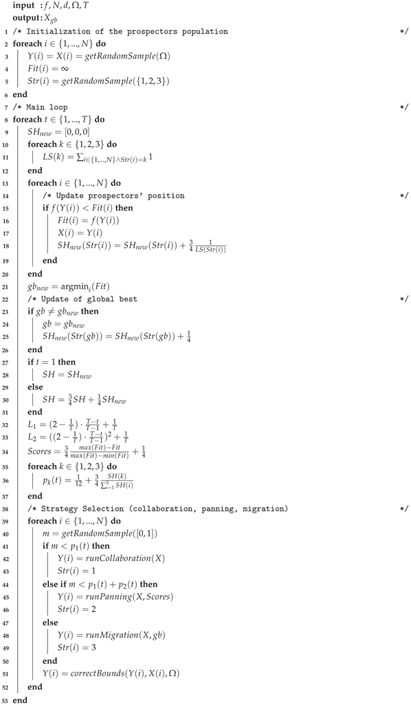 |
Initially, the population of prospectors X and their corresponding candidate positions Y are initialized randomly within the search space , while their fitness values are set to infinity. Furthermore, each prospector is assigned a random initial strategy , corresponding to Collaboration, Panning, and Migration, respectively.
In the main loop, which runs for T iterations, the algorithm first resets the temporary history of successful strategies . Then, it evaluates the candidate solutions. For each prospector i, if the new position yields a better fitness value than the current , the prospector moves to this new position () (see lines 15-19 of Algorithm 1). Crucially, this improvement triggers the adaptive reward mechanism: the strategy responsible for this success is rewarded by increasing its score in normalized by the number of prospectors using it (). This ensures that successful strategies used by fewer agents receive a higher relative reward.
Subsequently, the algorithm updates the global best solution by assigning the index of the best prospector to the variable (see lines 23-26 of Algorithm 1). If a new global optimum is found, the responsible strategy receives an additional fixed reward to further reinforce its probability of selection. The strategy history is then updated using a weighted moving average between the old history and the new rewards (), ensuring a smooth adaptation of probabilities over time. The factors and are updated based on the current iteration t, and a normalized fitness score vector () is calculated to guide the Panning process. The inclusion of the constant term in the Score definition (line 34, Algorithm 1) guarantees a non-zero selection probability even for the prospector with the worst fitness, thus enhancing the exploration capability of the method during the Panning phase.
Finally, as indicated in line 36 of Algorithm 1, the selection probabilities for the three strategies (Migration, Collaboration, Panning) are computed by combining the normalized values with a constant base probability. The probability distribution is defined as follows:
This formulation ensures that the probabilities sum to one (). Crucially, the inclusion of the constant term guarantees that all strategies remain accessible, preventing the complete exclusion of any strategy even if its historical performance score () drops to zero. Figure 4 presents a comparative qualitative analysis of AGRO and GRO, illustrating the evolution of the best fitness values for functions and of CBF23 suite defined in Section 4.1.1, alongside the temporal evolution of the probability distributions , , and . It is observed that AGRO obtains better scores than GRO, since the dynamic update mechanism ensures that all strategies remain accessible, while simultaneously assigning higher probability to the most promising strategy. Notably, the preferred strategy varies significantly over time, even in functions characterized by a single global minimum (see Figure 4a).
For the next iteration, each prospector selects a new strategy probabilistically based on (see lines 41-50 of Algorithm 1). More specifically:
- If Collaboration is selected, the new position is generated using the interaction between random agents.
- If Panning is selected, the algorithm utilizes the computed to guide the local search towards regions with better fitness, enhancing exploitation.
- If Migration is selected, the prospector moves towards the vicinity of the global best.
- Finally, a boundary control mechanism is applied: any proposed position that violates the search space limits is reverted to the prospector’s previous valid position (see line 51 of Algorithm 1).
4. Experimental Evaluation
In this section, the performance of the proposed Adaptive Gold Rush Optimizer (AGRO) is comprehensively evaluated. The algorithm is compared against ten state-of-the-art metaheuristic algorithms (see Table 1) utilizing three distinct sets of benchmark functions: the twenty-three classical benchmark functions, the CEC2017, and the CEC2019 [13]. These datasets provide a comprehensive assessment of the algorithm’s exploration, exploitation, and convergence capabilities across diverse optimization landscapes.
All the analysis has been done using MATLAB 2023b on an Intel i7 core 3.20GHz with 32 GB RAM without the use of code optimization or parallel processing tools. The code implementing the proposed methods along with the data sets will be publicly available online after acceptance of the paper: https://sites.google.com/site/costaspanagiotakis/research/agro.
4.1. Benchmark Test Functions
4.1.1. Classical Benchmark Functions
The first dataset comprises 23 classical benchmark functions [13] (CBF23), categorized into three groups:
- Unimodal Functions (): Characterized by a single global optimum, these functions evaluate the exploitation capability and convergence speed of the algorithm.
- Multimodal Functions (): These functions possess multiple local optima, testing the algorithm’s exploration ability and its robustness against premature convergence.
- Fixed-dimension Multimodal Functions (): These are lower-dimensional problems with fixed search spaces, designed to assess stability in constrained environments.
4.1.2. Classical Benchmark Functions
4.1.3. CEC2017 Benchmark
The CEC2017 benchmark dataset [13,30] consists of 30 complex functions () designed to simulate challenging real-world optimization problems. These functions are shifted, rotated, and shuffled to test the algorithm’s adaptability. The dataset is divided into four categories as shown in Table 5. The CEC2017 benchmark dataset was evaluated using a dimensionality of . In our experiments, the function has been removed from the CEC2017 set due to its unstable behavior [31].
4.1.4. CEC2019 Benchmark
4.2. Evaluation Metrics
To provide a comprehensive and fair assessment of the proposed algorithm’s performance, standard statistical metrics are employed following the methodology established in recent state-of-the-art studies [9,10,13,25,26]. Each algorithm is executed for independent runs for every benchmark function to mitigate the stochastic nature of metaheuristic optimization and the maximum number of iterations is . These parameter settings are consistent with those commonly adopted in state-of-the-art methods [9,13,25]. The following metrics are recorded and analyzed:
The primary indicators of performance are the Best, Average (Mean) and the Standard Deviation (SD) of the optimal fitness values recorded across independent runs.
- : This metric indicates the best score of the algorithm. It is calculated as:where represents the best fitness value found in the i-th run.
- : This metric indicates the accuracy of the algorithm and its ability to converge to the global optimum. This is the most important and robust metric and it is calculated as:
- Standard Deviation (): This metric evaluates the stability and robustness of the algorithm across different runs. A lower SD value indicates that the algorithm produces consistent results. It is defined as:
For each performance indicator, two key metrics are computed. The Ranking (, corresponding to the eleven comparative methods) and the Accuracy ().
- The Rank represents the average ranking of a method across all experiments according to the performance indicator used. Notably, a lower Rank indicates superior performance.
- The Accuracy metric quantifies the relative performance of a method normalized between the best and worst solutions found. It is formulated as:where v is the value obtained by the method, m corresponds to the best value found among all methods (minimum for minimization problems), and M represents the worst value (maximum value). Based on this definition, the top-performing method achieves , while the worst-performing one yields .
4.3. Performance Comparison of AGRO with Other Algorithms
In this section, a comprehensive comparative analysis is conducted to evaluate the efficiency of the proposed AGRO algorithm against ten state-of-the-art metaheuristics, including the original GRO. The experimental results are visualized in Figure 5 and summarized in Table 7, Table 8, Table 9, Table 10, Table 11 and Table 12.
Figure 5 provides a holistic view of the performance, illustrating the average Rank (top row) and Accuracy (bottom row) across all three datasets (CBF23, CEC2017, CEC2019) based on Mean metric. It is evident that AGRO yields the most stable and robust performance, maintaining the lowest rank and highest accuracy in most scenarios. More specifically, regarding the average rank criterion, AGRO demonstrates superior performance by the top position in the challenging CEC2017 and CEC2019 datasets, while ranking second in the CBF23 dataset. In terms of average accuracy, the proposed AGRO algorithm emerges as the leading optimizer, consistently achieving an average accuracy exceeding across all datasets. Notably, AGRO outperforms GRO, in all scenarios, highlighting the efficacy of the proposed modifications, particularly the adaptive mechanism, which significantly enhances the prospectors’ ability to explore the search space effectively.
Table 7, Table 8 and Table 9 report numerical results on the average ranking of the algorithms based on Best, Mean, and Standard Deviation (SD) metrics under the CBF23 dataset, the CEC2017 suite, and the CEC2019 suite, respectively. The algorithms are arranged in descending order based on the Mean criterion. Regarding the Best criterion, AGRO ranks as the second-best method on the CBF23 and CEC2017 suites, and third on the CEC2019 dataset. In terms of the Mean and Standard Deviation (SD) criteria, AGRO exhibits superior performance, by achieving the top position in the challenging CEC2017 and CEC2019 suites, while ranking second in the CBF23 dataset. Among competitor algorithms, BSLO, GRO, INFO, and PSO also demonstrate notable performance results.
Table 10, Table 11 and Table 12 report numerical results on the average accuracy of the algorithms computed by the Best and Mean metrics under the CBF23 dataset, the CEC2017 suite, and the CEC2019 suite, respectively. The algorithms are arranged in descending order based on the Mean criterion. Regarding the Best criterion, AGRO ranks as the third-best method on the CBF23 suite, and second best method on the CEC2017 and CEC2019 datasets. In terms of the Mean criterion, AGRO exhibits superior performance, by the top position in any dataset. Among competitor algorithms, BSLO, GRO, INFO, and PSO also demonstrate notable performance results.
These experimental findings, highlighted by the dominant performance of AGRO regarding the Mean and Standard Deviation criteria, demonstrate the robustness and ability to converge to the global optimum of the AGRO algorithm. Hereafter, we present more detailed results regarding the performance of the AGRO algorithm against ten state-of-the-art metaheuristics on each function of the three suites.
4.3.1. Results on Classical Benchmark Functions
The performance of the best comparative algorithms on the 23 classical benchmark functions (CBF23) is presented analytically in Table 13 and in Figure 6, via the average Rank that is computed on the Mean metric. As illustrated in Table 13, which presents the results of the five top-performing algorithms, AGRO demonstrates high exploitation capabilities. Specifically, it achieves optimal results in seven out of the ten Fixed-dimension Multimodal functions (refer to Table 4). Furthermore, the analysis of Figure 6 highlights the robustness of the proposed method, since AGRO attains high-performance results with an accuracy exceeding (based on the Mean metric) in 22 out of the 23 functions. BLSO achieves optimal results on all Unimodal Classical Benchmark functions (refer to Table 2) and Multimodal Classical Benchmark functions (refer to Table 3).
4.3.2. Results on CEC2017 Suite
The CEC2017 benchmark introduces greater complexity with shifted, rotated, hybrid, and composition functions. The performance of the best comparative algorithms on the CEC2017 benchmark is presented analytically in Table 14 and in Figure 7, based on the average Rank that is computed on the mean metric. As illustrated in Table 14, which summarizes the results of the top five methods, AGRO achieves the best results in 6 out of the 29 functions and secures the second-best position in 16 out of the 29 functions. Furthermore, the analysis of Figure 7 highlights the robustness of the proposed method. AGRO attains high-performance results with an accuracy exceeding (based on the Mean metric) in 26 out of the 29 functions. Similarly, GRO exhibits strong performance, reaching comparable accuracy levels in 24 out of the 29 functions.
4.3.3. Results on CEC2019 Suite
The CEC2019 benchmark tests the algorithms’ ability to locate the global optimum with extreme precision. The performance of the best comparative algorithms on the CEC2019 suite is presented analytically in Table 15 and in Figure 8, based on the average Rank that is computed on the mean metric. As illustrated in Table 15, which presents the results of the five top-performing algorithms, AGRO achieves best results in four out of the ten functions. Furthermore, the analysis of Figure 7 highlights the robustness of the proposed method, since AGRO attains high-performance results with an accuracy exceeding (based on the Mean metric) in eight out of the ten functions. GRO also achieves high performance results with accuracy exceeding (based on the Mean metric) in seven out of ten functions.
5. Conclusions
In this paper, a novel metaheuristic algorithm named Adaptive Gold Rush Optimizer (AGRO) was proposed as a substantial evolution of the standard Gold Rush Optimizer (GRO). The primary motivation behind AGRO was to address the structural limitations of GRO, specifically the inherent bias towards zero coordinates and the static nature of its strategy selection process. To this end, AGRO introduced fundamental modifications to the search equations and incorporated a dynamic strategy selection mechanism that adaptively prioritizes the most effective search behaviors (Migration, Collaboration, or Panning) based on their real-time contribution to the solution quality.
The performance of AGRO was evaluated against ten state-of-the-art algorithms, including the original GRO, BLSO, PSO, INFO, BLSO, GWO and other recent metaheuristics, across three diverse benchmark suites: the 23 Classical Benchmark Functions (CBF23), the CEC2017 suite, and the CEC2019 suite. The experimental results demonstrated that AGRO exhibits superior robustness and efficiency. Specifically:
- In terms of exploration, AGRO successfully avoided premature convergence in complex multimodal landscapes of CBF23 and CEC2017, significantly outperforming algorithms with static parameters.
- In terms of exploitation and precision, the algorithm achieved remarkable accuracy in the CEC2019 dataset, often locating the global optimum with high precision where other methods stagnated.
- Comparative analysis confirmed that AGRO consistently achieved the lowest average rank and highest accuracy across the majority of test functions, validating the effectiveness of the proposed adaptive mechanism.
Furthermore, the qualitative analysis revealed that the dynamic probability update allows the algorithm to fluidly shift between exploration and exploitation, ensuring that the prospectors focus on the most promising regions of the search space.
Future research directions will focus on applying AGRO to complex real-world engineering design problems and constrained optimization tasks. Additionally, since the proposed adaptive strategy selection mechanism is generic, its integration into other metaheuristic frameworks to enhance their adaptability and performance constitutes a promising avenue for future study.
Author Contributions
The author confirms contribution to the paper as follows: Conceptualization, C.P.; Funding acquisition, C.P.; Investigation, C.P.; Methodology, C.P.; Software, C.P.; Validation, C.P.; Supervision, C.P.; Data Curation, C.P.; Writing – original draft, C.P.; Writing – review & editing, C.P.; reviewed the results and approved the final version of the manuscript. C.P.;
Institutional Review Board Statement
Not applicable
Informed Consent Statement
Not applicable
Data Availability Statement
The associated code and datasets are developed for the project can be shared publicly after the paper acceptance. The sharing of parts of the code or datasets could be approved, at the authors’ discretion, upon request.
Conflicts of Interest
The authors declare no conflict of interest.
References
- Zaher, H.; Al-Wahsh, H.; Eid, M.; Gad, R.S.; Abdel-Rahim, N.; Abdelqawee, I.M. A novel harbor seal whiskers optimization algorithm. Alexandria Engineering Journal 2023, 80, 88–109. [Google Scholar] [CrossRef]
- Yang, X.S. Nature-inspired metaheuristic algorithms; Luniver press, 2010.
- Rizk-Allah, R.M.; Saleh, O.; Hagag, E.A.; Mousa, A.A.A. Enhanced tunicate swarm algorithm for solving large-scale nonlinear optimization problems. International Journal of Computational Intelligence Systems 2021, 14, 189. [Google Scholar] [CrossRef]
- Rajwar, K.; Deep, K.; Das, S. An exhaustive review of the metaheuristic algorithms for search and optimization: Taxonomy, applications, and open challenges. Artificial Intelligence Review 2023, 56, 13187–13257. [Google Scholar] [CrossRef] [PubMed]
- Kennedy, J.; Eberhart, R. Particle swarm optimization. In Proceedings of the Proceedings of ICNN’95-International Conference on Neural Networks. IEEE, 1995, Vol. 4, pp. 1942–1948. [CrossRef]
- Rashedi, E.; Nezamabadi-Pour, H.; Saryazdi, S. GSA: A gravitational search algorithm. Information sciences 2009, 179, 2232–2248. [Google Scholar] [CrossRef]
- Mirjalili, S.; Mirjalili, S.M.; Lewis, A. Grey wolf optimizer. Advances in engineering software 2014, 69, 46–61. [Google Scholar] [CrossRef]
- Mirjalili, S.; Lewis, A. The whale optimization algorithm. Advances in engineering software 2016, 95, 51–67. [Google Scholar] [CrossRef]
- Ahmadianfar, I.; Heidari, A.A.; Nouri, N.; Chen, H. INFO: An efficient optimization algorithm based on weighted mean of vectors. Expert Systems with Applications 2022, 195, 116516. [Google Scholar] [CrossRef]
- Zolfi, K. Gold rush optimizer: A new population-based metaheuristic algorithm. Operations Research and Decisions 2023, 33, 113–150. [Google Scholar] [CrossRef]
- Rutenbar, R.A. Simulated annealing algorithms: An overview. IEEE Circuits and Devices magazine 2002, 5, 19–26. [Google Scholar] [CrossRef]
- Prajapati, V.K.; Jain, M.; Chouhan, L. Tabu search algorithm (TSA): A comprehensive survey. In Proceedings of the 2020 3rd International Conference on Emerging Technologies in Computer Engineering: Machine Learning and Internet of Things (ICETCE). IEEE, 2020, pp. 1–8.
- Bai, J.; Nguyen-Xuan, H.; Atroshchenko, E.; Kosec, G.; Wang, L.; Wahab, M.A. Blood-sucking leech optimizer. Advances in Engineering Software 2024, 195, 103696. [Google Scholar] [CrossRef]
- Črepinšek, M.; Liu, S.H.; Mernik, M. Exploration and exploitation in evolutionary algorithms: A survey. ACM computing surveys (CSUR) 2013, 45, 1–33. [Google Scholar] [CrossRef]
- Holland, J.H. Adaptation in natural and artificial systems: An introductory analysis with applications to biology, control, and artificial intelligence; MIT press, 1992.
- Es-Haghi, M.S.; Shishegaran, A.; Rabczuk, T. Evaluation of a novel Asymmetric Genetic Algorithm to optimize the structural design of 3D regular and irregular steel frames. Frontiers of Structural and Civil Engineering 2020, 14, 1110–1130. [Google Scholar] [CrossRef]
- Kirkpatrick, S.; Gelatt, C.D., Jr.; Vecchi, M.P. Optimization by simulated annealing. science 1983, 220, 671–680. [Google Scholar] [CrossRef] [PubMed]
- Storn, R.; Price, K. Differential evolution–a simple and efficient heuristic for global optimization over continuous spaces. Journal of global optimization 1997, 11, 341–359. [Google Scholar] [CrossRef]
- Dorigo, M.; Maniezzo, V.; Colorni, A. Ant system: Optimization by a colony of cooperating agents. IEEE transactions on systems, man, and cybernetics, part b (cybernetics) 1996, 26, 29–41. [Google Scholar] [CrossRef] [PubMed]
- Dorigo, M.; Birattari, M.; Stutzle, T. Ant colony optimization. IEEE computational intelligence magazine 2007, 1, 28–39. [Google Scholar] [CrossRef]
- Nadimi-Shahraki, M.H.; Taghian, S.; Mirjalili, S. An improved grey wolf optimizer for solving engineering problems. Expert Systems with Applications 2021, 166, 113917. [Google Scholar] [CrossRef]
- Heidari, A.A.; Mirjalili, S.; Faris, H.; Aljarah, I.; Mafarja, M.; Chen, H. Harris hawks optimization: Algorithm and applications. Future generation computer systems 2019, 97, 849–872. [Google Scholar] [CrossRef]
- Hashim, F.A.; Hussien, A.G. Snake Optimizer: A novel meta-heuristic optimization algorithm. Knowledge-Based Systems 2022, 242, 108320. [Google Scholar] [CrossRef]
- Mohammed, H.; Rashid, T. FOX: A FOX-inspired optimization algorithm. Applied Intelligence 2023, 53, 1030–1050. [Google Scholar] [CrossRef]
- Zhao, S.; Zhang, T.; Ma, S.; Chen, M. Dandelion Optimizer: A nature-inspired metaheuristic algorithm for engineering applications. Engineering Applications of Artificial Intelligence 2022, 114, 105075. [Google Scholar] [CrossRef]
- Fan, S.; Wang, R.; Su, K.; Song, Y.; Wang, R. A Sequoia-Ecology-Based Metaheuristic Optimisation Algorithm for Multi-Constraint Engineering Design and UAV Path Planning. Results in Engineering 2025, 105130. [Google Scholar] [CrossRef]
- Askari, Q.; Younas, I.; Saeed, M. Political Optimizer: A novel socio-inspired meta-heuristic for global optimization. Knowledge-based systems 2020, 195, 105709. [Google Scholar] [CrossRef]
- Minh, H.L.; Sang-To, T.; Wahab, M.A.; Cuong-Le, T. A new metaheuristic optimization based on K-means clustering algorithm and its application to structural damage identification. Knowledge-Based Systems 2022, 251, 109189. [Google Scholar] [CrossRef]
- Zhang, Y.; Jin, Z. Group teaching optimization algorithm: A novel metaheuristic method for solving global optimization problems. Expert Systems with Applications 2020, 148, 113246. [Google Scholar] [CrossRef]
- Awad, N.H.; Ali, M.Z.; Liang, J.; Qu, B.; Suganthan, P.N. Problem definitions and evaluation criteria for the CEC 2017 special session and competition on single objective bound constrained real-parameter numerical optimization. Technical report, Nanyang Technological University, Singapore, 2016.
- Trojovská, E.; Dehghani, M. A new human-based metahurestic optimization method based on mimicking cooking training. Scientific Reports 2022, 12, 14861. [Google Scholar] [CrossRef]
- Price, K.V.; Awad, N.H.; Ali, M.Z.; Suganthan, P.N. Problem definitions and evaluation criteria for the CEC 2019 special session and competition on single objective bound constrained real-parameter numerical optimization. Technical report, Nanyang Technological University, Singapore, 2018.
Figure 1.
A graphical representation illustrating two distinct search phases of metaheuristic algorithms: (a) exploration, characterized by discovering new regions using large steps, and (b) exploitation, focusing on refining the best solutions using small, fine steps.
Figure 1.
A graphical representation illustrating two distinct search phases of metaheuristic algorithms: (a) exploration, characterized by discovering new regions using large steps, and (b) exploitation, focusing on refining the best solutions using small, fine steps.
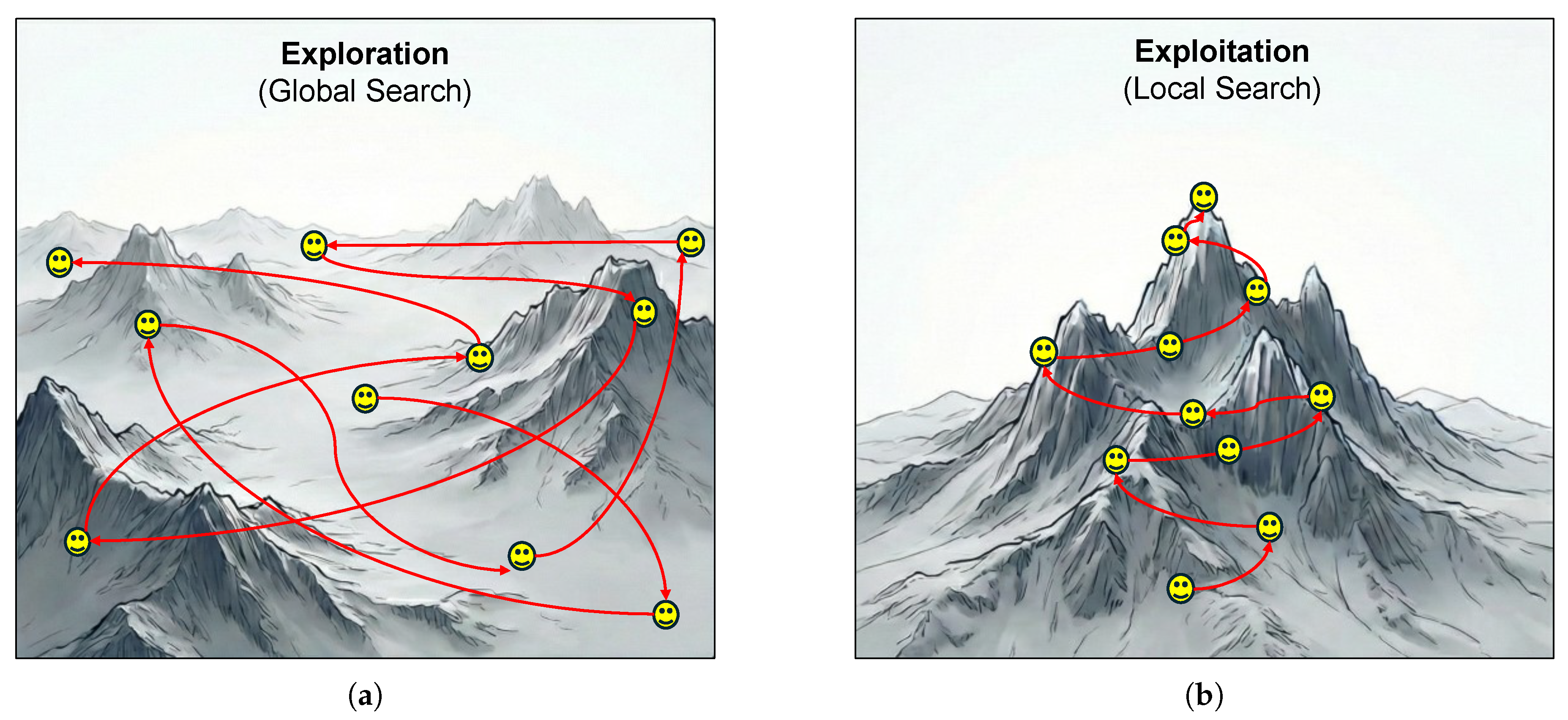
Figure 2.
The evolution of (a) , and the range of (b) and (c) during the execution of GRO.
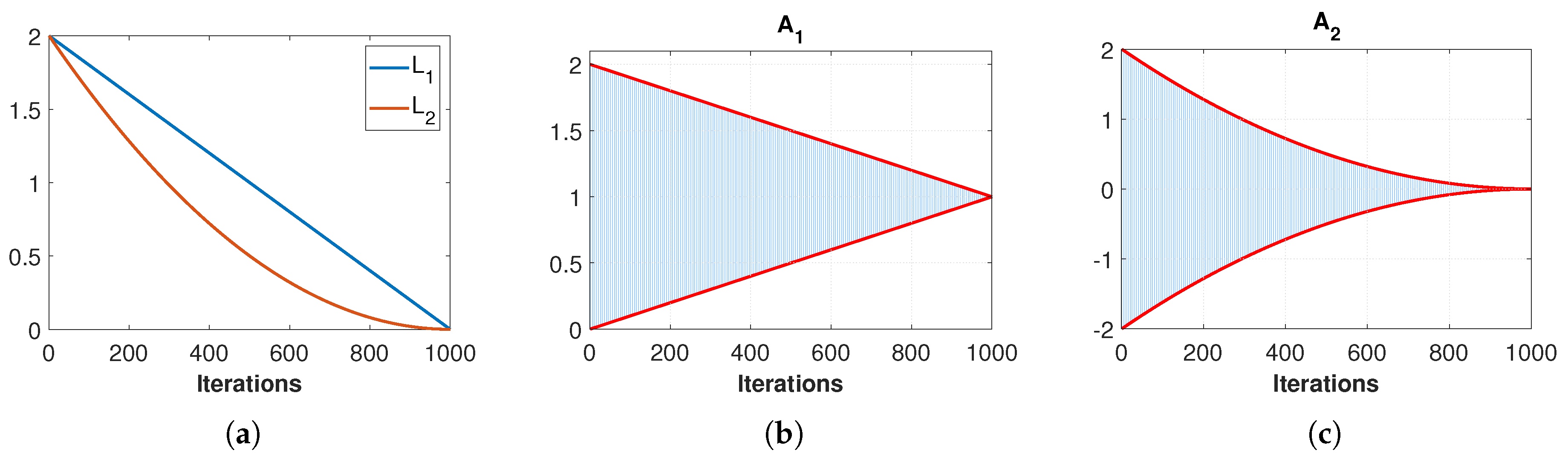
Figure 3.
The schematic representation of the three phases of GRO, (a) migration, (b) collaboration and (c) panning.
Figure 3.
The schematic representation of the three phases of GRO, (a) migration, (b) collaboration and (c) panning.
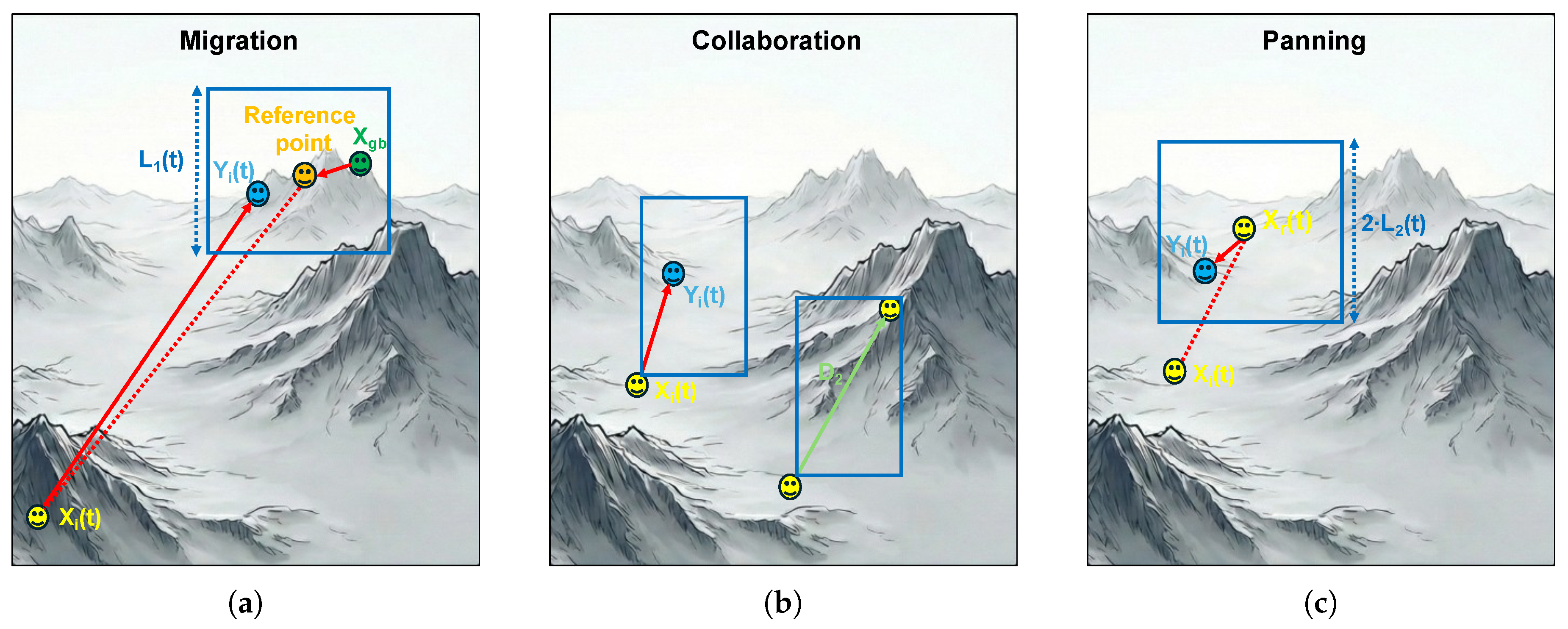
Figure 4.
Qualitative analysis for the (a) and (c) functions from the CBF23 suite. The evolution of probability distributions , and for the (b) and (d) .
Figure 4.
Qualitative analysis for the (a) and (c) functions from the CBF23 suite. The evolution of probability distributions , and for the (b) and (d) .
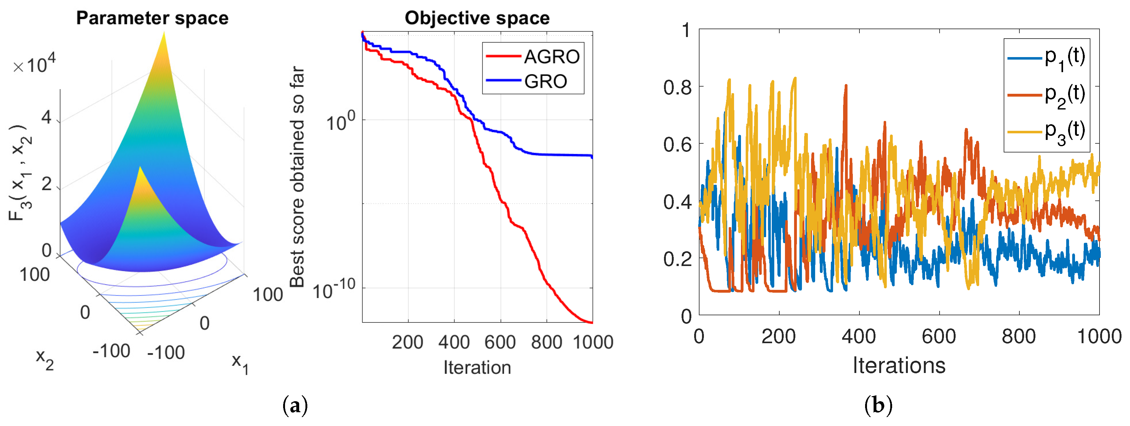
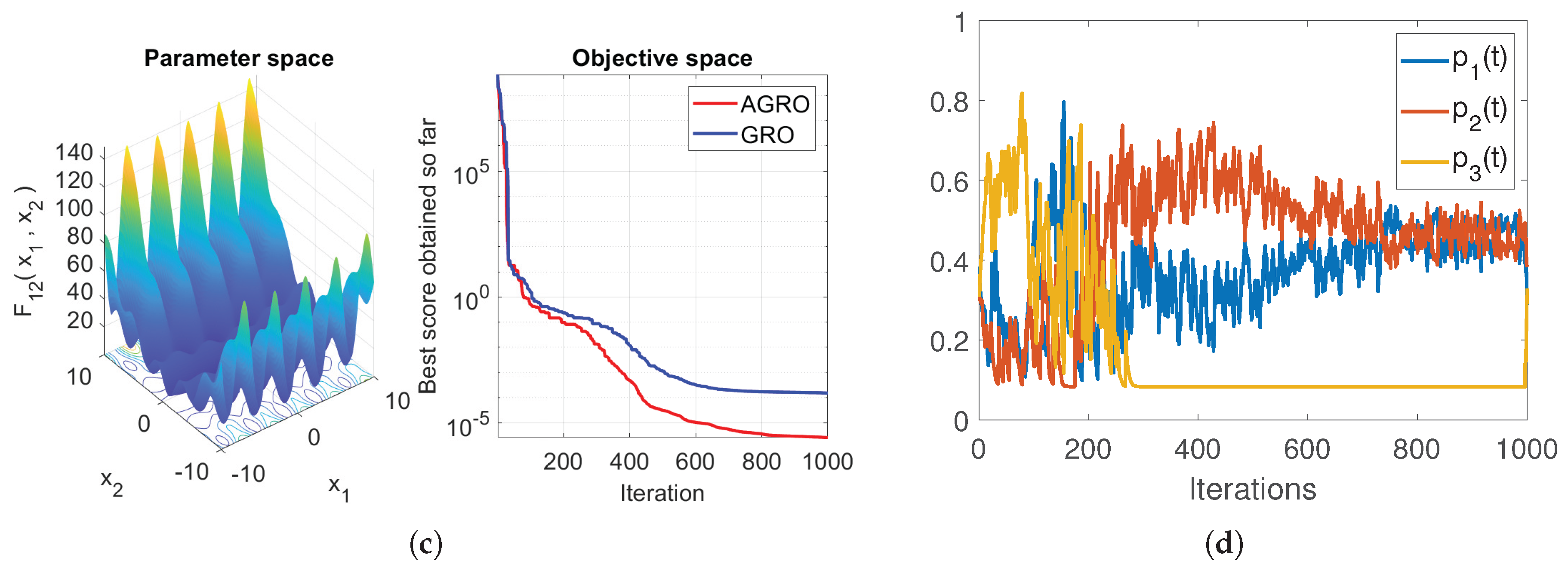
Figure 5.
The average rank (top) and average accuracy (bottom) based on Mean metric for the eleven algorithms evaluated on (a) the 23 Classical Benchmark Functions, (b) the CEC2017 dataset, and (c) the CEC2019 dataset.
Figure 5.
The average rank (top) and average accuracy (bottom) based on Mean metric for the eleven algorithms evaluated on (a) the 23 Classical Benchmark Functions, (b) the CEC2017 dataset, and (c) the CEC2019 dataset.
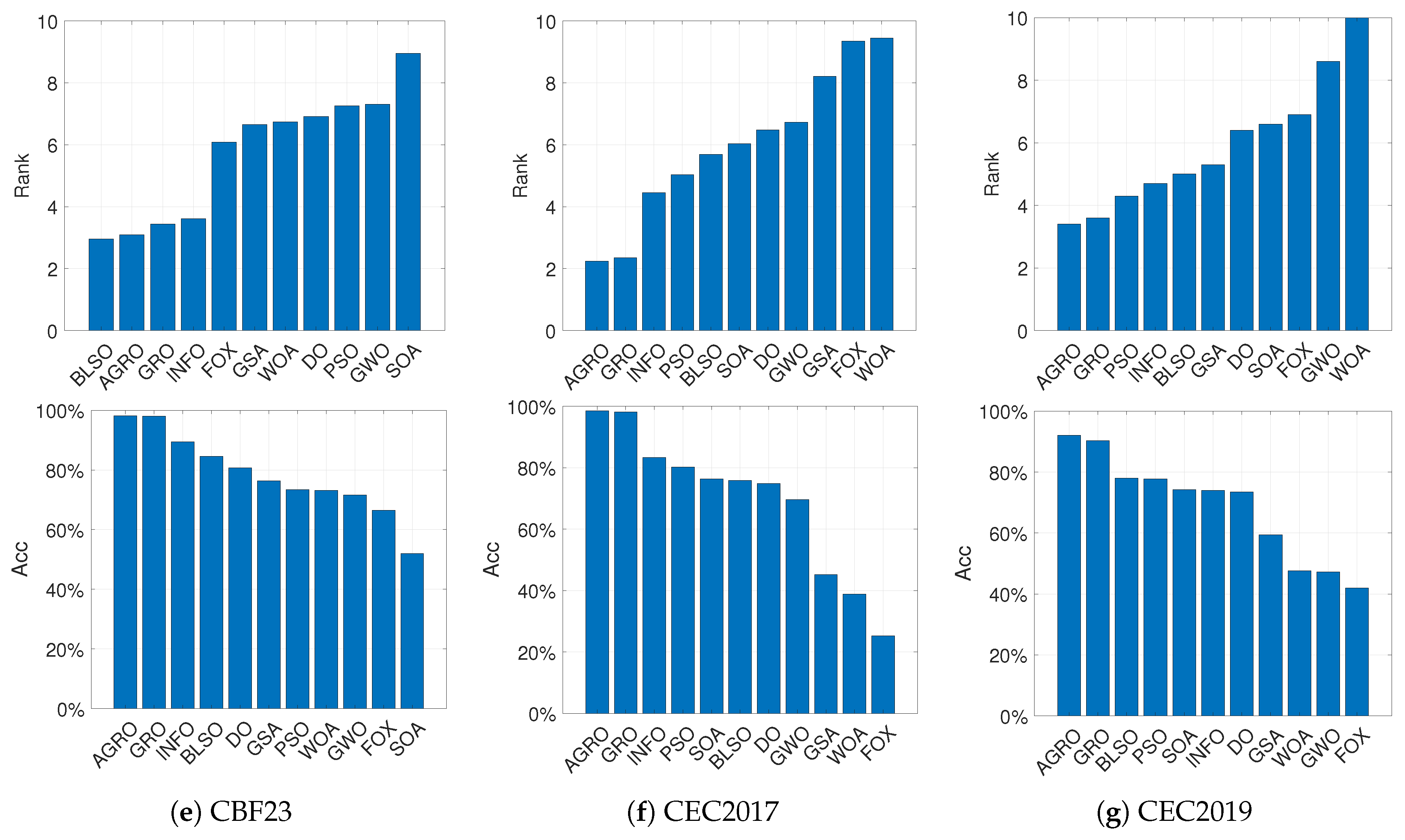
Figure 6.
Rank (top) and Accuracy (bottom) based on Mean metric of the top three performing algorithms for each of the 23 Classical Benchmark Functions.
Figure 6.
Rank (top) and Accuracy (bottom) based on Mean metric of the top three performing algorithms for each of the 23 Classical Benchmark Functions.
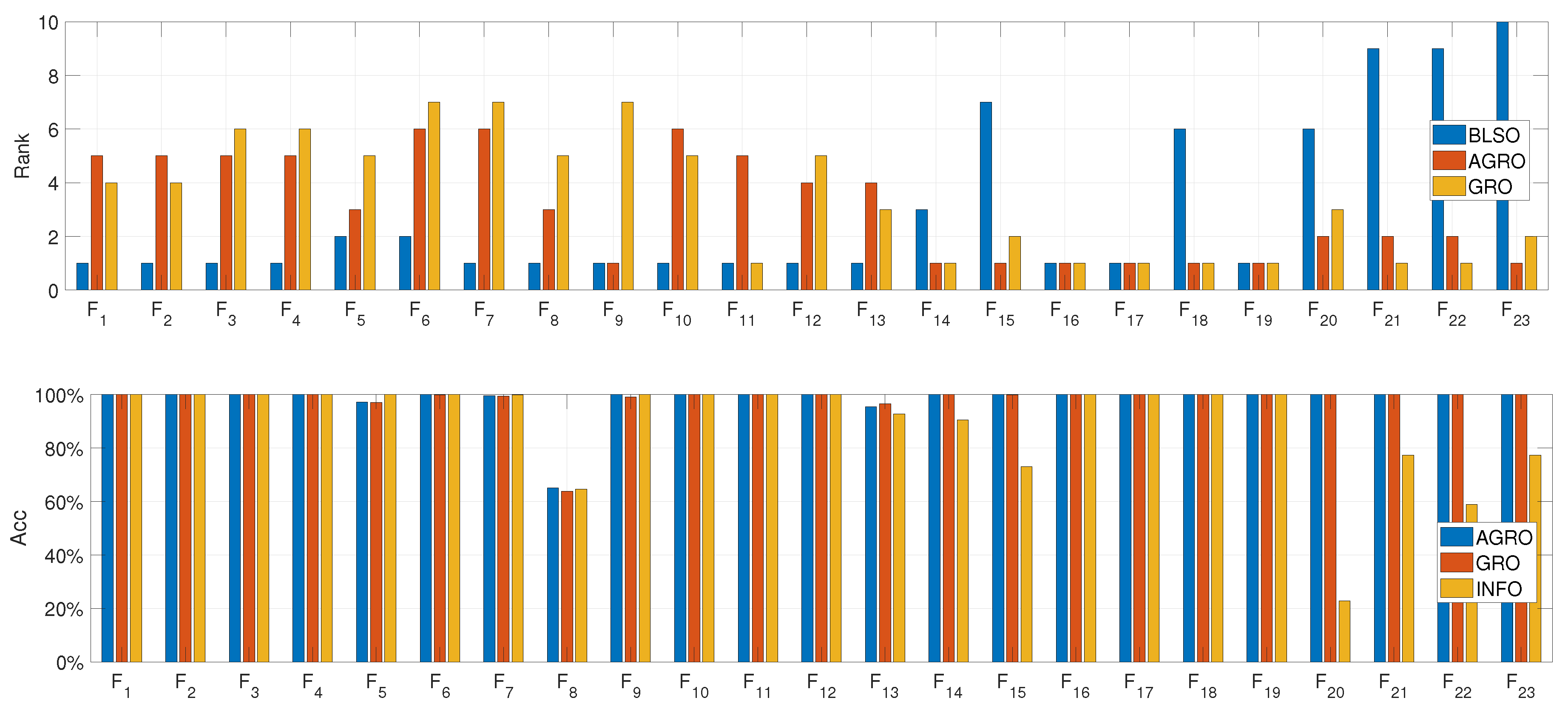
Figure 7.
Rank (top) and Accuracy (bottom) based on Mean metric of the top three performing algorithms across the 29 functions of the CEC2017 dataset.
Figure 7.
Rank (top) and Accuracy (bottom) based on Mean metric of the top three performing algorithms across the 29 functions of the CEC2017 dataset.
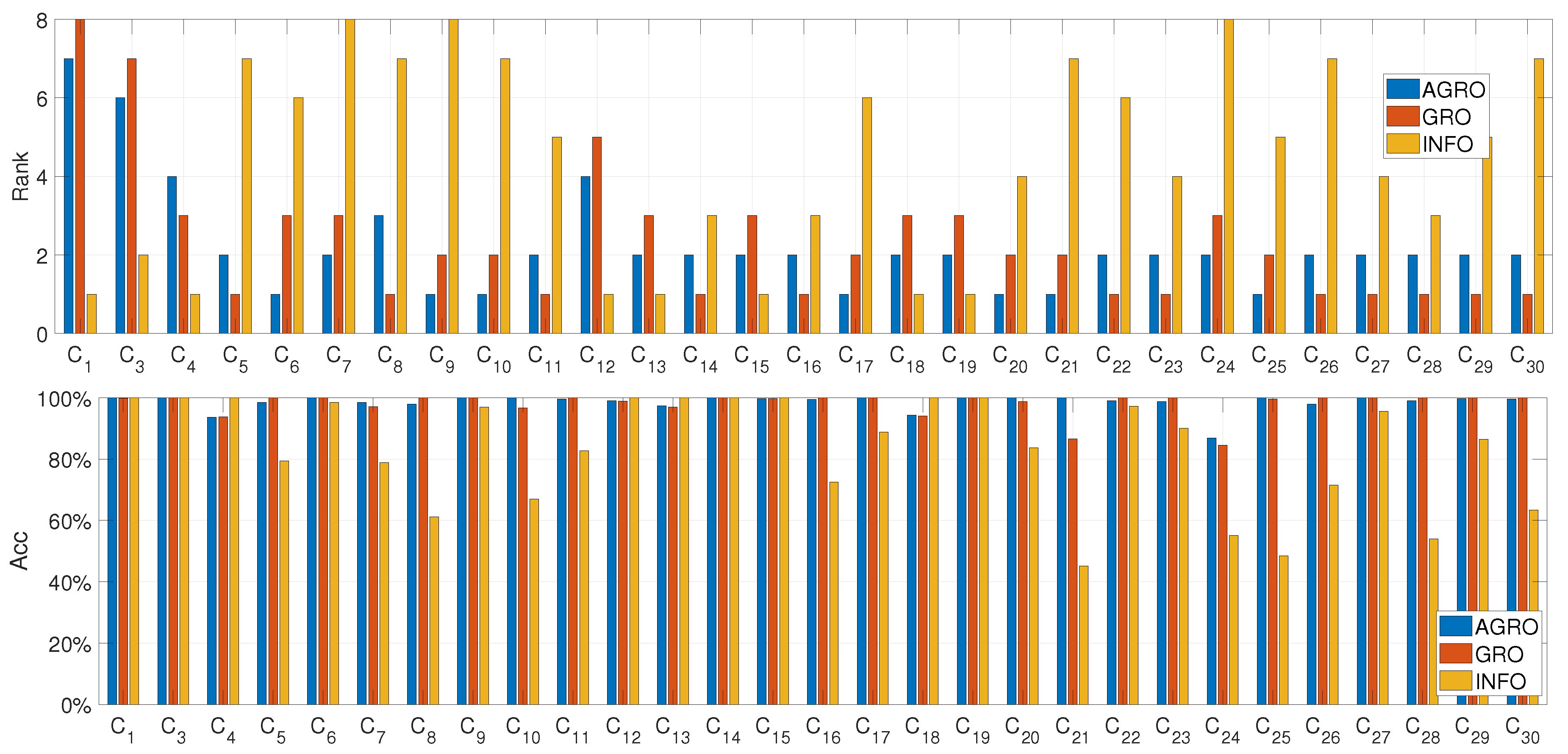
Figure 8.
Rank (top) and Accuracy (bottom) based on Mean metric of the top three performing algorithms across the 10 functions of the CEC2019 dataset.
Figure 8.
Rank (top) and Accuracy (bottom) based on Mean metric of the top three performing algorithms across the 10 functions of the CEC2019 dataset.
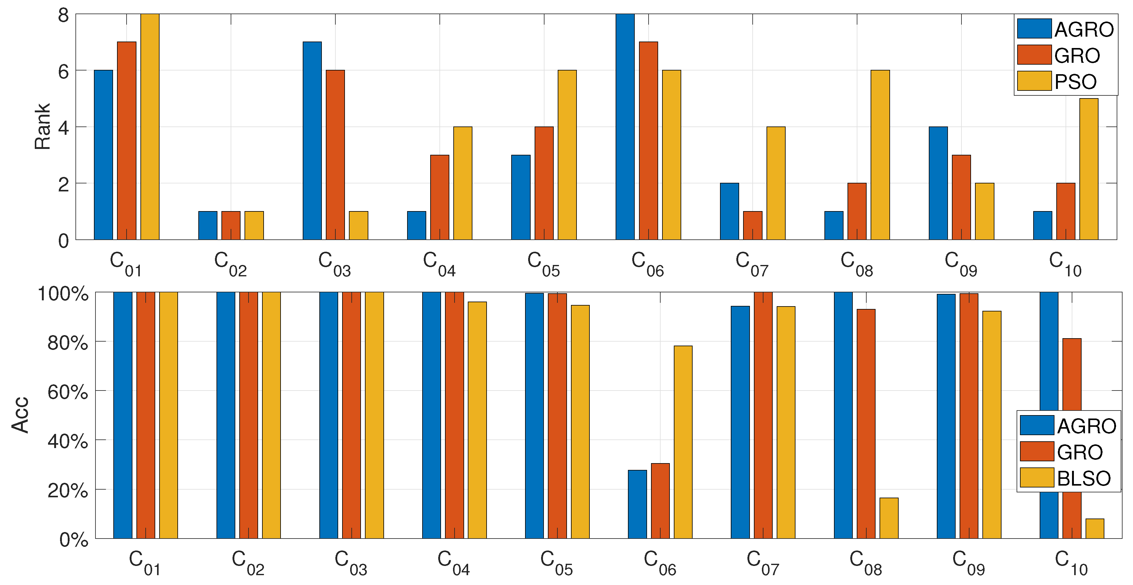

Table 1.
Overview of the optimization algorithms considered in this study.
| Acronym | Algorithm Name | Mechanism | Year |
|---|---|---|---|
| PSO | Particle Swarm Optimization [5] | Animals (birds): Mimics the behavior of bird flocks. | 1995 |
| GSA | Gravitational Search Algorithm [6] | Physics (masses): Based on the law of gravity and mass interactions. | 2009 |
| GWO | Grey Wolf Optimizer [7] | Animals (grey wolves): Mimics the leadership hierarchy and hunting mechanism of grey wolves in nature. | 2014 |
| WOA | Whale Optimization Algorithm [8] | Animals (Whales): Mimics the bubble-net hunting strategy of humpback whales. | 2016 |
| DO | Dandelion Optimizer [25] | Plants (dandelion seed): Inspired by the dissemination of dandelion seeds carried by the wind. | 2022 |
| FOX | FOX Optimizer [24] | Animals (fox): Mimics the foraging behavior of foxes in nature when hunting prey. | 2022 |
| INFO | Weighted Mean of Vectors [9] | Computational Geometry: Based on vector operations (weighted mean). | 2022 |
| GRO | Gold Rush Optimizer [10] | Human (gold prospectors): Mimics the behavior of gold prospectors during the Gold Rush era. | 2023 |
| BLSO | Blood-sucking Leech Optimizer [13] | Animals (leeches): Mimics the blood-sucking foraging behaviour of leeches. | 2024 |
| SOA | Sequoia Optimization Algorithm [26] | Plants (Sequoia): Inspired by the self-regulating and restorative phenomena observed in sequoia forest ecosystems. | 2025 |
Table 2.
Unimodal Classical Benchmark Functions ().
| ID | Function | Range | |
|---|---|---|---|
| 0 | |||
| 0 | |||
| 0 | |||
| 0 | |||
| 0 | |||
| 0 | |||
| 0 |
Table 3.
Multimodal Classical Benchmark Functions ().
| ID | Function | Range | |
|---|---|---|---|
| 0 | |||
| 0 | |||
| 0 | |||
| 0 | |||
| 0 |
Table 4.
Fixed-dimension Multimodal Classical Benchmark Functions.
| ID | Function | Dim (d) | Range | |
|---|---|---|---|---|
| 2 | ||||
| 4 | ||||
| 2 | ||||
| 2 | ||||
| 2 | 3 | |||
| 3 | ||||
| 6 | ||||
| 4 | ||||
| 4 | ||||
| 4 |
Table 5.
Summary of CEC2017 Benchmark Functions. Search Range: .
| Type | Functions | Description |
|---|---|---|
| Unimodal | Shifted and Rotated Unimodal Functions | |
| Multimodal | Shifted and Rotated Multimodal Functions | |
| Hybrid | Combinations of unimodal and multimodal sub-functions | |
| Composition | Merging properties of multiple sub-functions |
Table 6.
CEC2019 Benchmark Functions (100-Digit Challenge).
| Function | Function Name | Dim (d) | Range | |
|---|---|---|---|---|
| Storn’s Chebyshev Polynomial | 9 | 1 | ||
| Inverse Hilbert Matrix | 16 | 1 | ||
| Lennard-Jones Minimum Energy | 18 | 1 | ||
| Rastrigin | 10 | 1 | ||
| Griewank | 10 | 1 | ||
| Weierstrass | 10 | 1 | ||
| Modified Schwefel | 10 | 1 | ||
| Expanded Schaffer F6 | 10 | 1 | ||
| Happy Cat | 10 | 1 | ||
| Ackley | 10 | 1 |
Table 7.
Average ranking of the algorithms in terms of Best, Mean, and Standard Deviation (SD) metrics on the CBF23 dataset. The algorithms are arranged in descending order based on the Mean criterion.
Table 7.
Average ranking of the algorithms in terms of Best, Mean, and Standard Deviation (SD) metrics on the CBF23 dataset. The algorithms are arranged in descending order based on the Mean criterion.
| Rank | Algorithm | Best | Mean | SD |
|---|---|---|---|---|
| 1 | BLSO | 3.00 | 2.96 | 2.78 |
| 2 | AGRO | 3.43 | 3.09 | 3.78 |
| 3 | GRO | 3.43 | 3.43 | 3.74 |
| 4 | INFO | 2.09 | 3.61 | 4.65 |
| 5 | FOX | 5.83 | 6.09 | 4.61 |
| 6 | GSA | 5.83 | 6.65 | 6.48 |
| 7 | WOA | 7.13 | 6.74 | 7.48 |
| 8 | DO | 6.74 | 6.91 | 6.96 |
| 9 | PSO | 4.26 | 7.26 | 7.91 |
| 10 | GWO | 7.57 | 7.30 | 7.26 |
| 11 | SOA | 10.57 | 8.96 | 8.65 |
Table 8.
Average ranking of the algorithms in terms of Best, Mean, and Standard Deviation (SD) metrics on the CEC2017 dataset. The algorithms are arranged in descending order based on the Mean criterion.
Table 8.
Average ranking of the algorithms in terms of Best, Mean, and Standard Deviation (SD) metrics on the CEC2017 dataset. The algorithms are arranged in descending order based on the Mean criterion.
| Rank | Algorithm | Best | Mean | SD |
|---|---|---|---|---|
| 1 | AGRO | 3.24 | 2.24 | 2.86 |
| 2 | GRO | 3.52 | 2.34 | 3.03 |
| 3 | INFO | 2.72 | 4.45 | 4.86 |
| 4 | PSO | 4.34 | 5.03 | 5.17 |
| 5 | BLSO | 5.28 | 5.69 | 6.34 |
| 6 | SOA | 6.66 | 6.03 | 5.31 |
| 7 | DO | 6.93 | 6.48 | 6.45 |
| 8 | GWO | 7.48 | 6.72 | 6.45 |
| 9 | GSA | 8.34 | 8.21 | 6.90 |
| 10 | FOX | 8.17 | 9.34 | 9.21 |
| 11 | WOA | 9.14 | 9.45 | 9.41 |
Table 9.
Average ranking of the algorithms in terms of Best, Mean, and Standard Deviation (SD) metrics on the CEC2019 dataset. The algorithms are arranged in descending order based on the Mean criterion.
Table 9.
Average ranking of the algorithms in terms of Best, Mean, and Standard Deviation (SD) metrics on the CEC2019 dataset. The algorithms are arranged in descending order based on the Mean criterion.
| Rank | Algorithm | Best | Mean | SD |
|---|---|---|---|---|
| 1 | AGRO | 4.3 | 3.4 | 4.5 |
| 2 | GRO | 3.7 | 3.6 | 4.9 |
| 3 | PSO | 3.4 | 4.3 | 4.7 |
| 4 | INFO | 4.3 | 4.7 | 5.9 |
| 5 | BLSO | 4.9 | 5.0 | 4.9 |
| 6 | GSA | 5.8 | 5.3 | 4.9 |
| 7 | DO | 6.2 | 6.4 | 6.2 |
| 8 | SOA | 7.6 | 6.6 | 6.8 |
| 9 | FOX | 7.0 | 6.9 | 6.4 |
| 10 | GWO | 7.8 | 8.6 | 7.7 |
| 11 | WOA | 9.7 | 10.0 | 8.4 |
Table 10.
Average accuracy of the algorithms computed by the Best and Mean metrics on the CBF23 dataset. The algorithms are arranged in ascending order based on the Mean criterion.
Table 10.
Average accuracy of the algorithms computed by the Best and Mean metrics on the CBF23 dataset. The algorithms are arranged in ascending order based on the Mean criterion.
| Rank | Algorithm | Best | Mean |
|---|---|---|---|
| 1 | AGRO | 98.13% | 98.14% |
| 2 | GRO | 97.65% | 98.05% |
| 3 | INFO | 98.52% | 89.43% |
| 4 | BLSO | 98.92% | 84.54% |
| 5 | DO | 97.64% | 80.72% |
| 6 | GSA | 84.53% | 76.32% |
| 7 | PSO | 95.42% | 73.46% |
| 8 | WOA | 87.39% | 73.18% |
| 9 | GWO | 77.66% | 71.65% |
| 10 | FOX | 96.42% | 66.42% |
| 11 | SOA | 20.71% | 51.93% |
Table 11.
Average accuracy of the algorithms computed by the Best and Mean metrics on the CEC2017 dataset. The algorithms are arranged in ascending order based on the Mean criterion.
Table 11.
Average accuracy of the algorithms computed by the Best and Mean metrics on the CEC2017 dataset. The algorithms are arranged in ascending order based on the Mean criterion.
| Rank | Algorithm | Best | Mean |
|---|---|---|---|
| 1 | AGRO | 94.19% | 98.58% |
| 2 | GRO | 95.39% | 98.15% |
| 3 | INFO | 85.00% | 83.33% |
| 4 | PSO | 85.69% | 80.20% |
| 5 | SOA | 80.73% | 76.39% |
| 6 | BLSO | 81.98% | 75.83% |
| 7 | DO | 75.50% | 74.88% |
| 8 | GWO | 74.15% | 69.67% |
| 9 | GSA | 30.45% | 45.25% |
| 10 | WOA | 52.99% | 38.83% |
| 11 | FOX | 54.51% | 25.28% |
Table 12.
Average accuracy of the algorithms computed by the Best and Mean metrics on the CEC2019 dataset. The algorithms are arranged in ascending order based on the Mean criterion.
Table 12.
Average accuracy of the algorithms computed by the Best and Mean metrics on the CEC2019 dataset. The algorithms are arranged in ascending order based on the Mean criterion.
| Rank | Algorithm | Best | Mean |
|---|---|---|---|
| 1 | AGRO | 90.95% | 92.05% |
| 2 | GRO | 92.16% | 90.35% |
| 3 | BLSO | 81.42% | 77.99% |
| 4 | PSO | 88.69% | 77.78% |
| 5 | SOA | 70.80% | 74.27% |
| 6 | INFO | 81.71% | 73.96% |
| 7 | DO | 80.09% | 73.53% |
| 8 | GSA | 58.22% | 59.43% |
| 9 | WOA | 43.32% | 47.57% |
| 10 | GWO | 62.07% | 47.24% |
| 11 | FOX | 52.99% | 42.00% |
Table 13.
Statistical comparison of the top five algorithms on the CBF23 functions based on the average Rank that is computed on the mean metric.
Table 13.
Statistical comparison of the top five algorithms on the CBF23 functions based on the average Rank that is computed on the mean metric.
| Function | Metric | BLSO | AGRO | GRO | INFO | FOX |
|---|---|---|---|---|---|---|
| Mean | 0.00E+00 | 6.19E-76 | 2.54E-131 | 5.67E-55 | 0.00E+00 | |
| SD | 0.00E+00 | 2.88E-75 | 9.94E-131 | 2.53E-55 | 0.00E+00 | |
| Mean | 0.00E+00 | 8.11E-48 | 4.51E-83 | 2.92E-27 | 0.00E+00 | |
| SD | 0.00E+00 | 2.33E-47 | 1.74E-82 | 7.29E-28 | 0.00E+00 | |
| Mean | 0.00E+00 | 5.47E-04 | 2.42E-01 | 8.65E-52 | 0.00E+00 | |
| SD | 0.00E+00 | 2.05E-03 | 8.66E-01 | 1.67E-51 | 0.00E+00 | |
| Mean | 0.00E+00 | 9.01E-05 | 2.84E-04 | 5.23E-28 | 0.00E+00 | |
| SD | 0.00E+00 | 2.89E-04 | 1.26E-03 | 2.75E-28 | 0.00E+00 | |
| Mean | 2.53E+01 | 2.55E+01 | 2.60E+01 | 1.97E+01 | 2.88E+01 | |
| SD | 1.04E-01 | 3.25E-01 | 1.92E-01 | 8.76E-01 | 4.07E-02 | |
| Mean | 2.50E-15 | 1.75E-04 | 1.32E-03 | 6.30E-12 | 2.73E-03 | |
| SD | 6.96E-16 | 1.94E-04 | 1.86E-03 | 3.45E-11 | 1.13E-03 | |
| Mean | 4.88E-05 | 2.20E-03 | 3.82E-03 | 5.68E-04 | 5.60E-05 | |
| SD | 5.47E-05 | 1.42E-03 | 2.66E-03 | 4.05E-04 | 5.19E-05 | |
| Mean | -1.26E+04 | -9.09E+03 | -8.96E+03 | -9.05E+03 | -7.01E+03 | |
| SD | 8.22E-11 | 7.67E+02 | 6.12E+02 | 7.39E+02 | 6.10E+02 | |
| Mean | 0.00E+00 | 0.00E+00 | 1.10E+00 | 0.00E+00 | 0.00E+00 | |
| SD | 0.00E+00 | 0.00E+00 | 5.04E+00 | 0.00E+00 | 0.00E+00 | |
| Mean | 4.44E-16 | 6.60E-15 | 4.12E-15 | 4.44E-16 | 4.44E-16 | |
| SD | 0.00E+00 | 1.60E-15 | 6.49E-16 | 0.00E+00 | 0.00E+00 | |
| Mean | 0.00E+00 | 8.34E-04 | 0.00E+00 | 0.00E+00 | 0.00E+00 | |
| SD | 0.00E+00 | 3.23E-03 | 0.00E+00 | 0.00E+00 | 0.00E+00 | |
| Mean | 3.13E-16 | 7.91E-06 | 4.99E-05 | 4.30E-15 | 6.84E-05 | |
| SD | 1.02E-16 | 1.06E-05 | 4.45E-05 | 1.51E-14 | 2.05E-05 | |
| Mean | 3.33E-15 | 2.19E-02 | 1.66E-02 | 3.54E-02 | 1.00E-01 | |
| SD | 1.15E-15 | 4.10E-02 | 3.37E-02 | 4.73E-02 | 5.43E-01 | |
| Mean | 9.98E-01 | 9.98E-01 | 9.98E-01 | 1.91E+00 | 1.06E+01 | |
| SD | 1.13E-16 | 0.00E+00 | 0.00E+00 | 2.50E+00 | 3.97E+00 | |
| Mean | 8.24E-04 | 3.10E-04 | 3.21E-04 | 1.77E-03 | 3.71E-04 | |
| SD | 3.80E-04 | 4.38E-06 | 3.02E-05 | 5.06E-03 | 2.32E-04 | |
| Mean | -1.03E+00 | -1.03E+00 | -1.03E+00 | -1.03E+00 | -9.77E-01 | |
| SD | 5.05E-16 | 6.78E-16 | 6.78E-16 | 6.65E-16 | 2.07E-01 | |
| Mean | 3.98E-01 | 3.98E-01 | 3.98E-01 | 3.98E-01 | 3.98E-01 | |
| SD | 0.00E+00 | 0.00E+00 | 0.00E+00 | 0.00E+00 | 1.08E-10 | |
| Mean | 3.00E+00 | 3.00E+00 | 3.00E+00 | 3.00E+00 | 1.29E+01 | |
| SD | 2.50E-14 | 1.42E-15 | 1.26E-15 | 1.22E-15 | 2.51E+01 | |
| Mean | -3.86E+00 | -3.86E+00 | -3.86E+00 | -3.86E+00 | -3.86E+00 | |
| SD | 1.82E-15 | 2.71E-15 | 2.71E-15 | 2.71E-15 | 1.19E-07 | |
| Mean | -3.27E+00 | -3.32E+00 | -3.32E+00 | -3.27E+00 | -3.25E+00 | |
| SD | 5.99E-02 | 2.19E-14 | 4.20E-10 | 6.03E-02 | 5.96E-02 | |
| Mean | -5.76E+00 | -1.02E+01 | -1.02E+01 | -9.15E+00 | -5.74E+00 | |
| SD | 2.38E+00 | 3.77E-08 | 6.33E-12 | 2.60E+00 | 1.76E+00 | |
| Mean | -6.24E+00 | -1.04E+01 | -1.04E+01 | -8.21E+00 | -5.62E+00 | |
| SD | 2.89E+00 | 1.48E-13 | 1.51E-15 | 3.43E+00 | 1.62E+00 | |
| Mean | -6.28E+00 | -1.05E+01 | -1.05E+01 | -9.51E+00 | -6.03E+00 | |
| SD | 3.21E+00 | 1.98E-15 | 1.14E-15 | 2.66E+00 | 2.05E+00 |
Table 14.
Statistical comparison of the top five algorithms on the CEC2017 functions based on the average Rank that is computed on the mean metric.
Table 14.
Statistical comparison of the top five algorithms on the CEC2017 functions based on the average Rank that is computed on the mean metric.
| Function | Metric | AGRO | GRO | INFO | PSO | SOA |
|---|---|---|---|---|---|---|
| Mean | 5.47E+03 | 1.52E+04 | 1.00E+02 | 2.00E+03 | 2.17E+04 | |
| SD | 1.33E+04 | 3.51E+04 | 1.38E-02 | 1.89E+03 | 7.08E+03 | |
| Mean | 3.02E+02 | 3.04E+02 | 3.00E+02 | 3.00E+02 | 5.78E+03 | |
| SD | 4.41E+00 | 7.28E+00 | 4.01E-11 | 8.77E-14 | 3.33E+03 | |
| Mean | 4.03E+02 | 4.03E+02 | 4.00E+02 | 4.03E+02 | 4.05E+02 | |
| SD | 1.70E+00 | 1.77E+00 | 1.71E-01 | 9.76E-01 | 2.03E+00 | |
| Mean | 5.09E+02 | 5.07E+02 | 5.25E+02 | 5.23E+02 | 5.14E+02 | |
| SD | 2.92E+00 | 2.62E+00 | 1.02E+01 | 9.97E+00 | 8.33E+00 | |
| Mean | 6.00E+02 | 6.00E+02 | 6.01E+02 | 6.03E+02 | 6.00E+02 | |
| SD | 3.34E-04 | 8.90E-04 | 1.37E+00 | 8.03E+00 | 2.80E-01 | |
| Mean | 7.18E+02 | 7.19E+02 | 7.37E+02 | 7.27E+02 | 7.22E+02 | |
| SD | 2.61E+00 | 3.71E+00 | 1.31E+01 | 7.18E+00 | 5.75E+00 | |
| Mean | 8.09E+02 | 8.08E+02 | 8.21E+02 | 8.19E+02 | 8.08E+02 | |
| SD | 3.90E+00 | 2.87E+00 | 9.89E+00 | 7.85E+00 | 4.32E+00 | |
| Mean | 9.00E+02 | 9.00E+02 | 9.26E+02 | 9.00E+02 | 9.00E+02 | |
| SD | 1.94E-06 | 1.77E-05 | 4.96E+01 | 5.90E-01 | 2.67E-02 | |
| Mean | 1.32E+03 | 1.37E+03 | 1.77E+03 | 1.73E+03 | 1.69E+03 | |
| SD | 2.19E+02 | 1.87E+02 | 3.08E+02 | 2.83E+02 | 2.46E+02 | |
| Mean | 1.10E+03 | 1.10E+03 | 1.12E+03 | 1.13E+03 | 1.11E+03 | |
| SD | 1.11E+00 | 1.04E+00 | 1.78E+01 | 2.50E+01 | 5.16E+00 | |
| Mean | 4.06E+04 | 4.78E+04 | 7.50E+03 | 1.28E+04 | 1.10E+06 | |
| SD | 3.55E+04 | 5.77E+04 | 1.21E+04 | 1.17E+04 | 9.80E+05 | |
| Mean | 1.97E+03 | 2.06E+03 | 1.47E+03 | 1.02E+04 | 9.66E+03 | |
| SD | 3.07E+02 | 4.78E+02 | 1.92E+02 | 7.54E+03 | 4.50E+03 | |
| Mean | 1.44E+03 | 1.44E+03 | 1.45E+03 | 2.41E+03 | 5.17E+03 | |
| SD | 1.26E+01 | 1.38E+01 | 2.15E+01 | 9.86E+02 | 2.89E+03 | |
| Mean | 1.61E+03 | 1.62E+03 | 1.55E+03 | 2.74E+03 | 4.84E+03 | |
| SD | 4.81E+01 | 4.58E+01 | 4.59E+01 | 1.43E+03 | 2.55E+03 | |
| Mean | 1.61E+03 | 1.61E+03 | 1.76E+03 | 1.86E+03 | 1.82E+03 | |
| SD | 3.03E+01 | 2.18E+01 | 1.36E+02 | 1.07E+02 | 1.22E+02 | |
| Mean | 1.73E+03 | 1.73E+03 | 1.76E+03 | 1.78E+03 | 1.76E+03 | |
| SD | 9.52E+00 | 6.45E+00 | 4.81E+01 | 7.12E+01 | 3.22E+01 | |
| Mean | 3.31E+03 | 3.37E+03 | 1.86E+03 | 1.04E+04 | 6.94E+03 | |
| SD | 1.15E+03 | 1.08E+03 | 4.52E+01 | 8.09E+03 | 4.84E+03 | |
| Mean | 1.94E+03 | 1.96E+03 | 1.92E+03 | 4.78E+03 | 6.49E+03 | |
| SD | 1.83E+01 | 3.35E+01 | 1.48E+01 | 3.81E+03 | 3.95E+03 | |
| Mean | 2.01E+03 | 2.01E+03 | 2.06E+03 | 2.10E+03 | 2.09E+03 | |
| SD | 9.19E+00 | 1.02E+01 | 5.46E+01 | 6.26E+01 | 6.56E+01 | |
| Mean | 2.25E+03 | 2.27E+03 | 2.31E+03 | 2.30E+03 | 2.31E+03 | |
| SD | 5.44E+01 | 5.32E+01 | 4.46E+01 | 4.66E+01 | 1.80E+01 | |
| Mean | 2.29E+03 | 2.29E+03 | 2.30E+03 | 2.30E+03 | 2.30E+03 | |
| SD | 2.26E+01 | 2.54E+01 | 1.13E+00 | 7.88E-01 | 1.03E+00 | |
| Mean | 2.61E+03 | 2.61E+03 | 2.62E+03 | 2.63E+03 | 2.63E+03 | |
| SD | 4.11E+00 | 3.54E+00 | 1.08E+01 | 1.39E+01 | 1.55E+01 | |
| Mean | 2.67E+03 | 2.67E+03 | 2.75E+03 | 2.73E+03 | 2.75E+03 | |
| SD | 1.10E+02 | 1.02E+02 | 1.34E+01 | 7.84E+01 | 1.66E+01 | |
| Mean | 2.90E+03 | 2.90E+03 | 2.93E+03 | 2.93E+03 | 2.93E+03 | |
| SD | 8.18E+00 | 8.53E+00 | 2.26E+01 | 2.33E+01 | 2.05E+01 | |
| Mean | 2.90E+03 | 2.87E+03 | 3.22E+03 | 3.01E+03 | 3.33E+03 | |
| SD | 1.83E+01 | 7.76E+01 | 4.57E+02 | 3.68E+02 | 4.76E+02 | |
| Mean | 3.09E+03 | 3.09E+03 | 3.10E+03 | 3.12E+03 | 3.12E+03 | |
| SD | 2.45E+00 | 2.22E+00 | 1.91E+01 | 3.47E+01 | 2.34E+01 | |
| Mean | 3.14E+03 | 3.14E+03 | 3.28E+03 | 3.29E+03 | 3.34E+03 | |
| SD | 9.64E+01 | 9.64E+01 | 1.48E+02 | 1.44E+02 | 1.11E+02 | |
| Mean | 3.16E+03 | 3.16E+03 | 3.22E+03 | 3.23E+03 | 3.23E+03 | |
| SD | 1.28E+01 | 1.39E+01 | 6.67E+01 | 5.42E+01 | 5.24E+01 | |
| Mean | 2.12E+04 | 1.59E+04 | 5.34E+05 | 2.89E+05 | 2.81E+05 | |
| SD | 1.92E+04 | 9.01E+03 | 7.72E+05 | 4.92E+05 | 4.18E+05 |
Table 15.
Statistical comparison of the top five algorithms on the CEC2019 functions based on the average Rank that is computed on the mean metric.
Table 15.
Statistical comparison of the top five algorithms on the CEC2019 functions based on the average Rank that is computed on the mean metric.
| Function | Metric | AGRO | GRO | PSO | INFO | BLSO |
|---|---|---|---|---|---|---|
| Mean | 1.09E+08 | 1.16E+08 | 1.66E+08 | 1.56E+05 | 4.08E+04 | |
| SD | 1.32E+08 | 1.36E+08 | 1.35E+08 | 2.34E+05 | 1.49E+03 | |
| Mean | 1.73E+01 | 1.73E+01 | 1.73E+01 | 1.73E+01 | 1.73E+01 | |
| SD | 6.66E-15 | 6.53E-15 | 7.23E-15 | 7.23E-15 | 6.60E-10 | |
| Mean | 1.27E+01 | 1.27E+01 | 1.27E+01 | 1.27E+01 | 1.27E+01 | |
| SD | 4.81E-10 | 1.73E-10 | 3.61E-15 | 3.61E-15 | 3.61E-15 | |
| Mean | 7.85E+00 | 8.21E+00 | 2.18E+01 | 4.43E+01 | 4.49E+01 | |
| SD | 2.65E+00 | 3.34E+00 | 1.11E+01 | 3.27E+01 | 2.39E+01 | |
| Mean | 1.03E+00 | 1.04E+00 | 1.13E+00 | 1.12E+00 | 1.24E+00 | |
| SD | 1.59E-02 | 2.33E-02 | 8.91E-02 | 9.35E-02 | 1.46E-01 | |
| Mean | 7.98E+00 | 7.70E+00 | 5.71E+00 | 5.25E+00 | 3.11E+00 | |
| SD | 9.83E-01 | 1.07E+00 | 1.65E+00 | 2.15E+00 | 1.12E+00 | |
| Mean | 1.04E+02 | 7.66E+01 | 1.18E+02 | 2.76E+02 | 1.05E+02 | |
| SD | 1.01E+02 | 1.16E+02 | 1.29E+02 | 2.19E+02 | 1.23E+02 | |
| Mean | 2.68E+00 | 2.89E+00 | 5.09E+00 | 4.94E+00 | 5.20E+00 | |
| SD | 6.86E-01 | 7.91E-01 | 5.08E-01 | 1.09E+00 | 6.93E-01 | |
| Mean | 2.38E+00 | 2.37E+00 | 2.36E+00 | 2.40E+00 | 2.55E+00 | |
| SD | 2.35E-02 | 2.00E-02 | 1.68E-02 | 4.08E-02 | 1.20E-01 | |
| Mean | 1.50E+01 | 1.60E+01 | 1.94E+01 | 2.00E+01 | 2.00E+01 | |
| SD | 8.70E+00 | 7.80E+00 | 3.66E+00 | 3.48E-02 | 2.15E-02 |
Disclaimer/Publisher’s Note: The statements, opinions and data contained in all publications are solely those of the individual author(s) and contributor(s) and not of MDPI and/or the editor(s). MDPI and/or the editor(s) disclaim responsibility for any injury to people or property resulting from any ideas, methods, instructions or products referred to in the content. |
© 2026 by the authors. Licensee MDPI, Basel, Switzerland. This article is an open access article distributed under the terms and conditions of the Creative Commons Attribution (CC BY) license (http://creativecommons.org/licenses/by/4.0/).
Copyright: This open access article is published under a Creative Commons CC BY 4.0 license, which permit the free download, distribution, and reuse, provided that the author and preprint are cited in any reuse.


