
Submitted:
29 January 2026
Posted:
02 February 2026
You are already at the latest version
Abstract
Parallel electric-hydraulic hybrid (PEHH) powertrains offer benefits of lower energy consumption and increased battery lifetime compared to pure electric ones. These merits can be extended with advanced control methods that optimally deploy on-board energy sources. This work proposes a nonlinear model predictive control (NMPC) energy management strategy (EMS) for a PEHH wheel loader. The optimization minimizes energy usage and battery degradation by selecting the optimal power ratio between the electric and hydraulic subsystems. The state prediction is based on a discrete nonlinear dynamic model and an estimate of the future exogenous inputs developed from a high-fidelity digital-twin model of a wheel loader. The NMPC formulation is compared to a baseline rule-based EMS inspired by offline optimal control. The proposed NMPC results in 38.8\% less battery degradation and 7.5\% energy consumption reduction, even with 20\% error in the preview information. Hardware-in-the-loop (HiL) experiments validate our results and show that the NMPC EMS can be implemented in real-time, even with higher prediction error increasing the maximum computational time.
Keywords:
nonlinear model predictive control
; energy management
; hybrid electric vehicles
; wheel loader
1. Introduction
The growing concerns on emissions and the need for higher fuel economy, productivity, and reliability [1] as well as government mandates [2] are pushing off-road vehicles toward replacing diesel engines with alternative energy sources. Electric construction machinery has received increased attention since 2020 when industry prototypes were showcased, with a significant surge in 2022 with the introduction of the first products to the market [3]. Nonetheless, these machines face significant challenges including restricted on-board energy, especially for heavy-duty operations, high costs compared to the fuel-powered counterparts, and limited battery life [3].
Hybridizing the powertrain with hydraulic components has been shown to overcome these challenges in on-road vehicles. A particularly effective powertrain configuration for heavy-duty vehicles is parallel electric-hydraulic hybrid (PEHH). In one study, the driving range of an electric city bus is extended by 40% with a PEHH powertrain and the battery discharging stress of an electric delivery truck is reduced by 30% in PEHH configuration [4]. Another study shows that a PEHH semi-trailer truck has an extended battery lifespan and over 20% reduction in energy consumption compared to a fully electric vehicle [5].
These studies have confirmed that combining the high power density of a hydraulic system with the electric powertrain can increase the battery lifetime and decrease energy consumption for on-road vehicles. Off-road vehicles, particularly construction machinery such as wheel loaders which have cyclic operation with frequent direction changes, can similarly benefit from a PEHH powertrain. Zhang et al. [6] have shown that converting a battery electric wheel loader to a PEHH powertrain reduced the battery capacity fade by 7.61%. Additionally, Wang et al. [7] improved the productivity of the wheel loader operation by 17.4% with the hydraulic subsystem addition.
Developing an effective energy management strategy (EMS) is central to fully realizing the benefits of hybrid vehicle architectures. Significant efforts have been made in the past toward this topic [8,9]. The control strategy which defines the power-split ratio between the two power sources, can be classified into two categories: rule-based and optimization-based methods. Rule-based EMS determines the control input based on a set of pre-defined and condition-based strategies. These rules are developed based on experience, heuristics, or mathematical models [9]. Rule-based EMS is often employed commercially since it offers a simple design with minimal computational time [10]. However, rule-based EMS cannot provide an optimal strategy under a variety of operational requirements. Optimization-based EMS, on the other hand, determines the ideal strategy by solving an optimization problem subject to powertrain dynamics and operational constraints. The optimization problem is either solved globally offline or through real-time optimization. Dynamic programming (DP) and its derivatives are among popular approaches that solve for the globally optimum solution backward in time [11]. Nonetheless, to enable this optimal solution to be implemented in real-time, it must be converted into a set of rules [12]. Alternatively, real-time optimization-based methods solve optimization problems at each time step [9]. Notable methods include model predictive control (MPC) and equivalent consumption minimization strategy (ECMS) [13,14].
While ECMS minimizes a cost function only based on the current powertrain state and power demand, MPC uses an information preview and solves a constrained optimization problem over a finite, receding horizon, therefore providing a superior solution to ECMS. MPC improves on DP by being solvable in real-time and adapting to new conditions and MPC exceeds rule-based methods by finding a locally optimal solution and being robust to changes in operating condition. Therefore, significant attention has been paid toward the development of MPC-based EMS for vehicles with hybrid powertrains [15,16,17,18,19,20]. Notable examples include Deppen et al. [15] who have employed linear MPC to increase the fuel economy for an on-road parallel hydraulic hybrid vehicle by 48.5% compared to a non-hybrid vehicle. Vu et al. [16] increased the fuel economy for an on-road series hydraulic hybrid vehicle by 35% with a linear MPC EMS over a PID EMS. Curiel-Olivares et al. [17] developed a linear MPC for a series hybrid electric tractor which decreases fuel consumption by 12.17% while reducing battery degradation by 56.19% compared to a rule-based EMS. Serpi and Porru [18] presented an MPC-based EMS to minimize the operating costs of an HEV with a fuel cell, super capacitor, and battery pack. Wang and Jiao [19] have developed a multilevel MPC for energy management and engine tracking for a parallel hydraulic hybrid construction vehicle resulting in an improvement in miles per gallon of 7.3% compared to RB-PID strategy. Borhan et al. [20] have improved the fuel economy up to 10.7% with a nonlinear MPC EMS compared to commercial PSAT software for a power-split hybrid electric on-road vehicle.
For wheel loaders, Gao et al. [21] have generated a nonlinear MPC EMS which decreases the equivalent diesel consumption of a series hybrid electric wheel loader. Overall, the NMPC reduces the total economic cost by 5.12% compared to ECMS. For PEHH wheel loaders, rule-based EMS have been implemented which are designed manually from the preferred operation of the hydraulic and electric subsystems [6,7] or based on offline DP results in order to reduce costs associated with electricity and battery aging [22]. For on-road vehicles with a PEHH powertrain, neural networks have been trained offline to develop an EMS that minimizes the energy consumption rate [23]. Despite these significant advancements, to the best of the author’s knowledge, an MPC-based EMS for a PEHH wheel loader has not yet been developed.
The cyclic operation of wheel loaders is predictable and has frequent start-stops, which provides an ideal opening for predictive control. Additionally, including battery degradation in the cost function can surmount the aging challenge hindering the widespread adoption of the electric construction machinery. Therefore, this work:
- provides a control-friendly model for a PEHH wheel loader powertrain.
- formulates the nonlinear model predictive control problem which defines the energy management strategy by minimizing the energy usage and battery health degradation.
- evaluates the results of the NMPC EMS compared to a rule-based baseline EMS with realistic drive cycles from a digital-twin wheel loader model that captures accurate soil-tool interaction forces.
- validates the NMPC results for real-time operation through hardware-in-the-loop (HiL) simulation.
The rest of this paper is organized as follows: Section 2 describes the high-order model of the PEHH powertrain and the simplifications to formulate the optimization-friendly model. In Section 3 the rule-based baseline and NMPC energy management problem are introduced. In Section 4, the HiL simulation results are presented and discussed, and finally Section 5 summarizes the conclusions of this work.
2. System Modeling
This section details the modeling of the PEHH wheel loader pictured in Figure 1.
The electric and hydraulic subsystems of the powertrain operate in parallel to power the final drive of the vehicle. The powertrain includes the following components:
- Electric motor: A permanent magnet synchronous motor (PMSM) which has a wide torque-speed range and high power density [24].
- Battery: A lithium iron phosphate (LiFeP, LFP) battery that provides electrical energy to the motor and auxiliary components, including the hydraulic actuators that power the movement of the bucket. This chemistry is chosen for its slow aging and low risk of thermal runaway [25].
- Hydraulic pump/motor: A variable displacement pump/motor that operates in either pumping or motoring mode at various volumetric displacements.
- Accumulator: hydraulic accumulator which stores energy to power the hydraulic pump/motor.
2.1. High-Order Model for PEHH Powertrain
This section describes the high-order model developed to accurately describe dynamics of the PEHH wheel loader. To describe the full operation of the PEHH wheel loader, the model for each powertrain component is developed from experimentally validated sources and the duty cycle is described from a validated digital-twin model.
2.1.1. Vehicle Model
The vehicle dynamics describe the position, x, and velocity, v, of the wheel loader body as
where is the traction force provided by the powertrain, is the rolling resistance force, and is the force associated with impacting the soil pile. The total wheel loader mass, is defined as
where the vehicle mass, , includes the equivalent mass from rotational components, and is the mass of the soil in the bucket.
The rolling resistance is calculated as
where is the rolling resistance coefficient and g is the gravitational acceleration.
The traction force is described by
where is the torque on the wheels and is the radius of the wheels. The wheel torque is calculated as
where is the final drive ratio, is the traction efficiency. is the total powertrain torque provided by both the electric and hydraulic motor torque, and , respectively,
The power required at the wheel, , determines the direction of the flow of energy
where the angular velocity of the wheels, , is described as
A 1:1 gear ratio is assumed between the hydraulic and electric motors where they are connected to the final drive with a torque converter. Therefore, the angular velocity of the electric motor, , and hydraulic motor, , are given as
To analyze the operation of the wheel loaders, often a V-type loading cycle with simple forces are assumed [6,7]. However, in this work the wheel loader digging cycles are described from a validated digital-twin model of the wheel loader [26]. Figure 2(a) depicts the compact diesel wheel loader (ER-12) available at UC Davis Advanced Highway Maintenance and Construction Technology (AHMCT) research center, and Figure 2(b) displays the verified digital-twin model developed in [27] AGX Dynamics software by Karanfil et al. [28]. AGX Dynamics allows for modeling of soil interactions with both a volumetric and particle-based approach as well as physics-based multi-body dynamics. Thus, it is an ideal environment for the physics-based digital-twin that models the bucket-soil interactions during the digging cycle based on physical measurements from the ER-12 diesel wheel loader [28].
The position of the wheel loader is informed from experimental digging cycles to create the input for the Algoryx simulation. The digital-twin model then outputs the required forces based on specified soil parameters [29]. The drive cycle contains the following steps: (I) drive forward, (II) hit pile of material, scoop, and lift material, (III) reverse, (IV) turn and drive forward, (V) dump material, and (VI) return to the start of the cycle. The vehicle model then converts the variables of wheel loader position, thrust force, and soil pick-up mass, into the powertrain inputs of rotational speed of the motors, total torque requested, and required auxiliary power. For 10 digging cycles, the vehicle model inputs and powertrain inputs are shown in Figure 3.
2.1.2. Electric Motor Model
An electric motor model is developed based on the 2004 Toyota Prius 50 kW PMSM. The control action for the hybrid powertrain is the power-split ratio, , which describes the fraction of the total powertrain torque required from the electric motor. The vehicle is completely driven by the electric motor with a power split ratio of 1, and fully driven by the hydraulic motor at 0. Thus a value of from 0 to 1 requires the hydraulic and electric subsystems to be simultaneously powering the vehicle, while a value between 1 and 2 results in the battery powering the drive cycle and re-pressurizing the accumulator, and a negative from to 0 results in the hydraulic subsystem driving the wheels and recharging the battery.
The torque dynamics for the motor are modeled as
where is the first order motor time constant and is the produced torque.
The electrical power required by the electric motor involves including the motor/inverter efficiency, , as follows:
where the value of the the motor/inverter efficiency is described as a function of the angular velocity, , and torque, , based on the experimentally derived map by Oak Ridge National Laboratory (ORNL) [30] assuming axial scaling [31]. In regenerating mode, the electric motor has 1/2 the maximum torque and 1/2 the maximum power capacity compared to motoring mode [32].
2.1.3. Battery Model
The battery model describes electrical dynamics as an equivalent circuit model (ECM) based on experimental measurements and aging dynamics from a validated semi-empirical model. The battery provides power to the electric motor and the bucket hydraulics. Thus the battery power, is computed as
where describes the auxiliary power required to operate the lift and tilt cylinders.
The power required by each cell in the battery pack is assumed to be identical and given as
where is the number of cells connected in parallel and is the number of cells connected in series. The state of charge (SOC) of each battery cell is described through Coulomb counting as
where is the current applied to the cell, with battery discharging associated with a positive current, and is each cell’s nominal capacity in Ampere-hours (Ah).
The ECM describes the cell voltage, , as a combination of voltages across circuit components
where is the open circuit voltage, is the RC voltage, and the voltage across the internal resistance element is described with the current and the resistance, .
The RC voltage, , has dynamics of
based on values of the resistor, , and capacitor, . The values for , , , and are a function of the SOC and displayed in Figure 4. These dependencies are identified through experiments on a 25 Ah cell as detailed in the author’s previous work [33].
The battery cell’s power is described by
Battery health is correlated with the capacity of the battery and as the battery ages it loses some of its ability to store energy. The capacity fade of LFP type batteries relates to the loss of active lithium ions, which form a solid electrolyte interface (SEI) at the anode. To describe the battery aging, a model of the state of health (SOH) defined by Hu et al. [34] based on the semi-empirical model by Wang et al. [35] is deployed. This model captures the impacts of various temperatures, depth of discharge, and discharge rates on the capacity loss of LFP cells. A vehicle battery is defined to be at the end-of-life (EOL) when its capacity has degraded by 20%, therefore SOH ranges from 1 to 0 as the fresh battery degrades to its EOL.
The SOH is described by
where N is defined as the total number of charge-discharge cycles until EOL, computed as
where is the total ampere-hour throughput until EOL. The throughput is calculated as
where z is the constant power law factor with a value of 0.55. M is the pre-exponential factor and is the activation energy, which are both dependent on the c-rate, c, as defined by Wang et al. [35]. The c-rate describes the ratio between the cell current and the cell capacity as
The throughput is scaled by the ratio of the model’s cell capacity, , and the cell capacity for this work, [36].
2.1.4. Hydraulic Pump/Motor Model
The hydraulic pump/motor operates as a pump when converting mechanical energy into hydraulic energy and as a motor when converting hydraulic energy into mechanical energy. The variable displacement element controls the torque and flow rate directly. The torque provided by the hydraulic pump/motor is described as
where is the maximum volumetric displacement, is the pressure provided to the motor from the accumulator, and is the mechanical efficiency of the pump/motor. is the pump/motor displacement fraction which describes the variable displacement of the hydraulic pump/motor. The device is operating in pumping mode when and in motoring mode when [6].
The flow rate through the hydraulic pump/motor is modeled as
where is the volumetric efficiency of the pump/motor. The Parker Hannifin Corporation [37] outlines specified mechanical and volumetric efficiencies as a function of pressure and flow rate for pumps of various sizes. At any given time, the values for , and are produced from a look-up table modeled after the Parker Hannifin Corporation [37] plots.
2.1.5. Hydraulic Accumulator Model
The accumulator is composed of two sections, one which contains the hydraulic oil and the other is a gas bladder filled with an inert gas. As hydraulic oil flows into the accumulator, the pressure increases and the gas compresses. A polytropic quasi-static process models this process as
where , is the pressure of the gas, and is the volume of gas in the accumulator [22]. The gas and hydraulic oil are assumed to be at the same pressure, , which has dynamics of
found by taking the time derivative of Equation (25). is the pre-charged pressure of the accumulator which occurs at the total accumulator volume, [5].
The state of pressure of the accumulator, SOP, is defined to describe the fraction of pressure available from the accumulator as
where is the minimum working pressure and is the maximum pressure constrained by the hydraulic system design.
2.2. Control-Oriented Model
Nonlinear model predictive control requires a differentiable model that defines the components with discrete formulations. This section describes the simplifications made to the full-order model to transform it into one that can be used in an online optimization problem.
2.2.1. Electric Subsystem Model
The motor torque dynamics are faster than the NMPC sample times, therefore the motor torque is modeled as quasi-static
based on the input power-split ratio, , and the predicted total torque, at that time step (k). We convert the efficiency to a power loss function as
in which describes the powerloss through the electric motor. The powerloss is combination of polynomial and hyperbolic tangent function in angular velocity and torque at that time step as
where the values of the powerloss coefficients are described in Table 1.
The true powerloss and predicted powerloss are displayed in Figure 5 for every combination of electric motor angular velocity and torque. The model is shown to fall close to the exact prediction for various degrees of powerloss.
The battery cell’s current is computed as
which combines Equation (16) and Equation (18) in discrete time. To describe the dynamics of , the battery voltage is discretized assuming a zero-order hold approximation as
where is the length of each time step, specified as 0.1 seconds for the NMPC. The values of , , and are defined as constants from the battery model described in the author’s previous work [36] and given in Table 3.
Similarly, the future battery SOC is found as
Finally, the SOH of the battery is described by a similar formation as
2.2.2. Hydraulic Subsystem Model
The formulations for the hydraulic motor torque and volumetric flow rate are converted into torque loss and volumetric leakage functions as described in our previous work [36]
where the torque loss, , and volumetric leakage, are functions of the current pump/motor displacement fraction, the accumulator pressure, and angular velocity of the pump/motor. The functions are described as
where the values of the torque loss and volumetric leakage coefficients are described in Table 2.
The pressure dynamics of the accumulator are discretized assuming a zero-order hold with small pressure fluctuations
where is the same time step defined for the electrical subsystem.
The accumulator power, , at each time step is defined as
The control-oriented model parameters for the PEHH powertrain are described in Table 3.
2.2.3. Model Validation
The control-oriented model provides a simplified representation of the high-order model for feasible implementation in the optimization problem. Nonetheless, the optimal EMS relies on the accuracy of the control-oriented model. Figure 6 compares the simplified model and the high-order model for one representative wheel loader cycle.
As seen, the open-loop prediction of the control-oriented model closely follows the high-order one, even for 25 seconds of prediction. The maximum error in the battery SOC and accumulator SOP over the cycle is shown to be 0.017% and 0.021%, respectively. The maximum error of the battery SOH is very low at only 2.56E-7%. Thus, the nonlinear discrete control-oriented model can provide a valid prediction of future states with a 1 second prediction horizon for the model predictive control energy management strategy.
3. Energy Management
The energy management strategy specifies the power-split ratio between the electric and hydraulic subsystems at each time step. The battery is the main energy source, while the hydraulic system provides power to minimize battery aging and maximize system efficiency. This section first details the rule-based control that is used to provide a performance benchmark and then formulates the proposed nonlinear model predictive control framework.
3.1. Rule-Based Control
A rule-based controller determines the value of the input, the power-split ratio, based on a set of rules. Zhang et al. [6] have previously developed a rule-based scheme for a PEHH wheel loader which has driving and regenerating modes and keeps the accumulator state of pressure within a specified range. The algorithm employed in this work is presented in Figure 7 and is inspired by this methodology; however, this work allows for a larger range of the power-split ratio and thus there is more complexity to the defined rules. The author’s previous work solved the simultaneous design and optimal control problem for the PEHH wheel loader [36]. Thus, the optimal sizes from this work are used for this powertrain as described in Table 3 and the rule-based control is designed to mimic the optimal control results from this prior work.
The rule-based controller uses information on the current velocity, total torque required, and accumulator SOP to determine the value of the power-split ratio, . When in driving mode, if the velocity is low, the electric motor provides the required torque. Otherwise, the electric motor provides up to the maximum torque and then the excess is provided by the hydraulic pump/motor. In regenerating mode, if the velocity is low, the energy is funneled to the electric motor, but at high speeds, the torque re-pressurizes the hydraulic accumulator up to the maximum torque, at which point the excess energy will be received by the battery. Additionally, as Zhang et al. [6] have described, when the accumulator SOP is outside its limits, the powertrain will attempt to force it back inside such limits.
The rule based parameters include the following: the high pressure limit, , the low pressure limit, , the switching speed, , the maximum torque, , and the limiting torque, . The values of the rule-based parameters chosen to recreate the optimal control policy for the PEHH wheel loader [36] are shown in Table 4.
For one wheel loader cycle, the values of the input, , are shown in Figure 8 along with the rule-based mode defined for each time step. The controller tends to operate with purely hydraulic, mixed acceleration, or purely electric power, and rarely uses the hydraulic powertrain to charge the battery, or the electric powertrain to pressurize the accumulator since this energy flow introduces significant inefficiencies.
3.2. Nonlinear Model Predictive Control
Model predictive control uses a preview of the future inputs to define the optimal control input over a receding horizon by minimizing a cost function at each step. This requires a prediction of the future power demand and a discretized model of the system dynamics.
The optimization problem for NMPC minimizes the following cost function
where u represents the control input, the power-split ratio, and denotes the the state or input k steps ahead, given the current time, t. The first term in the cost function describes the total battery energy usage and the second term corresponds to the total accumulator energy over the prediction horizon. Positive power values relate to energy flowing out of the respective energy sources, and negative powers correspond with recharging the battery or repressurizing the accumulator. Weighting factors, and , penalize the battery aging and the deviation from the nominal SOP with values of 1E6 and 1E16, respectively. This work requires the accumulator to sustain its pressure and act as a pathway for energy savings, thus the SOP at the end of the cycles should not deviate significantly from the nominal SOP. The optimization is subject to the following constraints:
in which the state variable x includes , SOC, SOH, and SOP ( and Equation (42a) represents the nonlinear state transition equations defined by the discretized control-oriented model described in Equation (28) - Equation (39) and prediction of the exogenous inputs, . Additionally, Equation (42b) constrains the accumulator state of pressure to be within the same high and low limits developed in the rule-based scheme and detailed in Table 4. Equation (42c) constrains the battery state of charge to safe limits. Finally, Equation (42d) restricts the control input to the specified range from -1 to 2.
The exogenous inputs, w, describe the total traction torque, angular speed of the motors, and auxiliary power associated with each digging cycle, examples of which are shown in Figure 3. The problem step time, , is defined as 0.1 seconds and the prediction horizon, , is 10 steps.
The NMPC is evaluated for five scenarios: assuming perfect future knowledge of these exogenous inputs and a prediction error of 5, 10, 15, and 20%. The error in each exogenous input prediction is defined as a gaussian normal distribution with zero mean. The standard deviation is determined based on a fraction of the maximum value of that exogenous input throughout the cycles. This fraction is defined as the percentage error for each scenario. Note that the prediction of the wheel loader duty cycle is not a focus of this study. As mentioned, due to the repetitive nature of the wheel loader operations, such prediction models can be built from historical data as shown in existing literature [38,39]. In this work, instead we investigate the performance of the NMPC under significant errors in preview information. Nonetheless, we should emphasize that the preview information at a one second horizon can be acquired accurately as shown by Huang et al. [38]. In this work the noisy inputs are assigned as the actual inputs because the real-world wheel loader operation can include sudden acceleration-deceleration and sudden changes in requested torque and auxiliary power due to bucket-soil impacts, while data-driven prediction models often predict smoother profiles. Figure 9 displays one cycle of the wheel loader operation with the red line showing the predicted exogenous inputs and the blue line showing the actual values constructed by adding 20% error to the predicted values. In this case, the controller has some limited information on the cyclic nature of the exogenous inputs, but not the exact deviations.
The proposed optimization problem is solved using Matlab’s sequential quadratic programming (SQP) algorithm in fmincon.
4. Results
The NMPC problem solves a nonlinear optimization problem at each time step. Thus, it is imperative to test the real-time capabilities of the strategy. Hardware-in-the-loop (HiL) testing allows for real-time evaluation of the controller by separating the model of the plant and the model of the controller and simulating each in real-time. This provides a more practical simulation of applying the energy management strategy on the powertrain, since it accounts for computational limits on the controller and communication requirements.
The HiL test platform configuration is shown in Figure 10. The high-order model of the wheel loader powertrain described in Section 2.1. and the rule-based and NMPC controllers are developed in Simulink. These models are separated and converted to C-code using dSPACE Configuration Desk software. The dSPACE Control Desk software provides the testing environment that evaluates the plant model and controller individually and communicates the states and inputs between the two models. Table 5 displays the hardware specifications for the HiL testing.
For the 10 cycles of wheel loader operation, the rule-based and NMPC EMS are simulated on the high-order wheel loader model. The NMPC controller is tested for five preview scenarios: exact prediction, 5% prediction error, 10% prediction error, 15% prediction error, and 20% prediction error. The resulting power-split ratio, battery SOC, and accumulator SOP are compared in Figure 11 for the baseline rule-based controller and NMPC with exact prediction and a prediction error of 20%. As seen, the NMPC controller uses the accumulator far more than the rule-based controller. Consequently, the battery SOC fluctuates more and decreases more throughout the 10 cycles for the rule-based EMS compared to the NMPC controller. The final SOP for each case is not exactly the same as the initial value of 0.75, but the deviation is less than 2% for all cases. This ensures that the wheel loader operation is scalable to long working hours constrained only by the battery life.
Included in the cost function for the NMPC EMS is the battery degradation throughout the cycle. Figure 12 shows the battery SOH throughout the 10 cycles. For all proposed EMS, SOH is normalized with respect to the change in SOH for the rule-based case. Each NMPC controller has very similar battery aging, which is significantly lower than the rule-based energy management scheme. Even with 20% prediction error in the exogenous inputs, the NMPC EMS results in a 38.8% decrease in battery aging compared to the baseline rule-based EMS.
The algorithm for NMPC minimizes the total energy usage of the powertrain along with the battery aging, while keeping the accumulator SOP close to its nominal value. Thus, for a fair comparison of energy usage, it is assumed that the accumulator SOP must be returned to the nominal value using energy from the battery which is subject to losses through the electric motor and hydraulic pump/motor. The total energy usage includes the change in battery energy and the change in energy from the accumulator that is transferred to the battery. The total energy is calculated as
where is the battery energy difference and is the accumulator energy difference throughout the cycles. The energy difference for the accumulator is multiplied by the nominal efficiency of the hydraulic pump/motor system, , and the nominal efficiency of the electric motor, depending on the direction of the energy flow. The values for the nominal efficiencies are assumed to encapsulate the typical losses for energy flow through the hydraulic and electric systems without knowledge of the exact conditions of the energy transfer. Since the accumulator SOP is constrained to end close to its nominal value, the energy usage of the accumulator is significantly lower than the battery usage, thus these assumptions have negligible impact on the final energy usage.
Figure 13 displays the energy usage for each controller for the studied cycles, along with the percentage energy savings from the baseline rule-based case. The NMPC EMS which has perfect knowledge of the future cycle power requirements saves 22.7% of the total energy throughout the 10 cycles compared to the rule-based case, but even with reduced prediction precision, the NMPC EMS can still save 7.5% of the total energy. These results confirm that the NMPC EMS is more robust than one based on predetermined rules and thus can lead to significant benefits. These improvements include both a longer battery life and maximized operational time on a single battery charge which are both vital for construction vehicle electrification.
For the various levels of prediction error, the computation time for each controller step are shown in Figure 14. Every calculation has been completed in less than the step time of 100 ms, but when more error is introduced to the prediction, the maximum computation time increases to close to the step time.
Table 6 shows the minimum, maximum, and average compute time as well as standard deviation for NMPC with various levels of prediction error. The minimum and mean computation times differ slightly between each case, but the maximum computation time shows a significant increase with higher error levels. Additionally, the standard deviation in the computation time generally increases for higher error levels. Testing the NMPC with HiL experiments allows for real time application of the control system and thus proves that this algorithm can be implemented on real-world hardware.
5. Conclusions
In this paper, a nonlinear model predictive controller has been developed to manage the energy of a PEHH wheel loader. The performance of the NMPC EMS is compared for different levels of preview accuracy and against a baseline rule-based EMS developed from offline optimal control. All controllers are tested in real-time through hardware-in-the-loop simulations on a dSPACE SCALEXIO AutoBox. For all levels of prediction accuracy, the NMPC EMS outperforms the rule-based controller in battery aging and energy usage. However, higher errors in the prediction of exogenous inputs lead to decreased energy savings and longer maximum computational times.
Future work can investigate techniques to develop a linear model of the powertrain. Linear MPC inherently decreases computational time, but generally faces drawbacks from reduced model accuracy. Additionally, using prediction methods such as neural networks can produce robust previews for increasingly varied operational cycles. Pairing powertrain control with vehicle control can permit high accuracy in future predictions and increased energy savings.
Author Contributions
Conceptualization, S.N.; methodology, M.H.; investigation, M.H.; writing—original draft preparation, M.H.; writing—review and editing, S.N.; visualization, M.H.; supervision, S.N. All authors have read and agreed to the published version of the manuscript.
Funding
This research received no external funding.
References
- Beltrami, D.; Iora, P.; Tribioli, L.; Uberti, S. Electrification of compact off-highway vehicles—Overview of the current state of the art and trends. Energies 2021, 14, 5565. [Google Scholar] [CrossRef]
- Newsom, G. Exec. Order No. N-79-20, 2020.
- Huang, X.; Yan, W.; Cao, H.; Chen, S.; Tao, G.; Zhang, J. Prospects for purely electric construction machinery: Mechanical components, control strategies and typical machines. Automation in Construction 2024, 164, 105477. [Google Scholar] [CrossRef]
- Niu, G.; Shang, F.; Krishnamurthy, M.; Garcia, J.M. Design and analysis of an electric hydraulic hybrid powertrain in electric vehicles. IEEE Transactions on Transportation Electrification 2016, 3, 48–57. [Google Scholar] [CrossRef]
- Taaghi, A.; Yoon, Y. Optimal Control Co-Design of a Parallel Electric-Hydraulic Hybrid Vehicle. Technical report, SAE Technical Paper 2024-01-2154, 2024.
- Zhang, H.; Wang, F.; Xu, B.; Fiebig, W. Extending battery lifetime for electric wheel loaders with electric-hydraulic hybrid powertrain. Energy 2022, 261, 125190. [Google Scholar] [CrossRef]
- Wang, F.; Zhang, Q.; Wen, Q.; Xu, B. Improving productivity of a battery powered electric wheel loader with electric-hydraulic hybrid drive solution. Journal of Cleaner Production 2024, 440, 140776. [Google Scholar] [CrossRef]
- Xu, N.; Kong, Y.; Chu, L.; Ju, H.; Yang, Z.; Xu, Z.; Xu, Z. Towards a smarter energy management system for hybrid vehicles: A comprehensive review of control strategies. Applied sciences 2019, 9, 2026. [Google Scholar] [CrossRef]
- Panday, A.; Bansal, H.O. A review of optimal energy management strategies for hybrid electric vehicle. International Journal of Vehicular Technology 2014, 2014, 160510. [Google Scholar] [CrossRef]
- Hofman, T.; Steinbuch, M.; Van Druten, R.; Serrarens, A. Rule-based energy management strategies for hybrid vehicle drivetrains: A fundamental approach in reducing computation time. IFAC Proceedings Volumes 2006, 39, 740–745. [Google Scholar] [CrossRef]
- Nazari, S.; Siegel, J.; Stefanopoulou, A. Optimal energy management for a mild hybrid vehicle with electric and hybrid engine boosting systems. IEEE Transactions on Vehicular Technology 2019, 68, 3386–3399. [Google Scholar] [CrossRef]
- Pam, A.; Bouscayrol, A.; Fiani, P.; Noth, F. Rule-based energy management strategy for a parallel hybrid electric vehicle deduced from dynamic programming. In Proceedings of the 2017 IEEE Vehicle Power and Propulsion Conference (VPPC). IEEE, 2017; pp. 1–6.
- Nazari, S.; Middleton, R.; Siegel, J.; Stefanopoulou, A. Equivalent consumption minimization strategy for a power split supercharger. Technical report, SAE Technical Paper. 2019. [Google Scholar]
- Nazari, S.; Siegel, J.; Middleton, R.; Stefanopoulou, A. Power split supercharging: A mild hybrid approach to boost fuel economy. Energies 2020, 13, 6580. [Google Scholar] [CrossRef]
- Deppen, T.O.; Alleyne, A.G.; Stelson, K.; Meyer, J. A model predictive control approach for a parallel hydraulic hybrid powertrain. In Proceedings of the Proceedings of the 2011 American Control Conference. IEEE, 2011; pp. 2713–2718. [Google Scholar]
- Vu, T.V.; Chen, C.K.; Hung, C.W. A model predictive control approach for fuel economy improvement of a series hydraulic hybrid vehicle. Energies 2014, 7, 7017–7040. [Google Scholar] [CrossRef]
- Curiel-Olivares, G.; Escobar, G.; Johnson, S.; Schacht-Rodríguez, R. MPC-based EMS for a series hybrid electric tractor. IEEE Access 2024, 12, 135999–136010. [Google Scholar] [CrossRef]
- Serpi, A.; Porru, M. An MPC-based energy management system for a hybrid electric vehicle. In Proceedings of the 2020 IEEE vehicle power and propulsion conference (VPPC). IEEE; 2020; pp. 1–6. [Google Scholar]
- Wang, Z.; Jiao, X. Hierarchical model predictive control for hydraulic hybrid powertrain of a construction vehicle. Applied Sciences 2020, 10, 745. [Google Scholar] [CrossRef]
- Borhan, H.; Vahidi, A.; Phillips, A.M.; Kuang, M.L.; Kolmanovsky, I.V.; Di Cairano, S. MPC-based energy management of a power-split hybrid electric vehicle. IEEE Transactions on Control Systems Technology 2011, 20, 593–603. [Google Scholar] [CrossRef]
- Gao, R.; Zhou, G.; Wang, Q. Real-time three-level energy management strategy for series hybrid wheel loaders based on WG-MPC. Energy 2024, 295, 131011. [Google Scholar] [CrossRef]
- Zhang, H.; Wang, F.; Wu, J.; Xu, B.; Geimer, M. A Cycle-Adaptive Control Strategy to Minimize Electricity and Battery Aging Costs of Electric-Hydraulic Hybrid Wheel Loaders. Energy 2025, 134655. [Google Scholar] [CrossRef]
- Zhang, Z.; Zhang, T.; Hong, J.; Zhang, H.; Yang, J. Energy management strategy of a novel parallel electric-hydraulic hybrid electric vehicle based on deep reinforcement learning and entropy evaluation. Journal of Cleaner Production 2023, 403, 136800. [Google Scholar] [CrossRef]
- Hasnain, A.; Gamwari, A.S.; Resalayyan, R.; Sadabadi, K.F.; Khaligh, A. Medium and heavy duty vehicle electrification: Trends and technologies. IEEE Transactions on Transportation Electrification, 2024. [Google Scholar]
- Camargos, P.H.; dos Santos, P.H.; dos Santos, I.R.; Ribeiro, G.S.; Caetano, R.E. Perspectives on Li-ion battery categories for electric vehicle applications: a review of state of the art. International Journal of Energy Research 2022, 46, 19258–19268. [Google Scholar] [CrossRef]
- Karanfil, D. Developing Scalable Digital Twins of Construction Vehicles. PhD thesis, University of California, Davis, 2025. [Google Scholar]
- Algoryx. AGX Dynamics. 19 05 2025. Accessed: 2025-05-19. Available online: https://www.algoryx.se/agx-dynamics/.
- Karanfil, D.; Lindmark, D.; Servin, M.; Torick, D.; Ravani, B. Developing a calibrated physics-based digital twin for construction vehicles. arXiv preprint 2025, arXiv:2508.08576. [Google Scholar] [CrossRef]
- Abdolmohammadi, A.; Mojahed, N.; Nazari, S.; Ravani, B. Data-Efficient Excavation Force Estimation for Wheel Loaders. IEEE Access 2025, 13, 181846–181862. [Google Scholar] [CrossRef]
- Staunton, R.H.; Ayers, C.W.; Marlino, L.; Chiasson, J.; Burress, B. Evaluation of 2004 Toyota Prius hybrid electric drive system. Technical report, Oak Ridge National Lab.(ORNL), Oak Ridge, TN (United States), 2006.
- Stipetic, S.; Zarko, D.; Popescu, M. Ultra-fast axial and radial scaling of synchronous permanent magnet machines. IET Electric Power Applications 2016, 10, 658–666. [Google Scholar] [CrossRef]
- Schauer, E.; Moskalik, A.; Kargul, J.; Stuhldreher, M.; Butters, K.; Barba, D.; Drallmeier, J.; Gross, M. Development of Benchmarking Methods for Electric Vehicle Drive Units. Technical report, SAE Technical Paper; 2024. [Google Scholar]
- Haas, M.; Nemati, A.; Moura, S.; Nazari, S. LiFePO4 Battery Thermal Modeling: Bus Bar Thermal Effects. IFAC-PapersOnLine 2024, 58, 887–892. [Google Scholar] [CrossRef]
- Hu, X.; Perez, H.E.; Moura, S.J. Battery charge control with an electro-thermal-aging coupling. Proceedings of the Dynamic Systems and Control Conference. American Society of Mechanical Engineers 2015, Vol. 57243, V001T13A002. [Google Scholar]
- Wang, J.; Liu, P.; Hicks-Garner, J.; Sherman, E.; Soukiazian, S.; Verbrugge, M.; Tataria, H.; Musser, J.; Finamore, P. Cycle-life model for graphite-LiFePO4 cells. Journal of power sources 2011, 196, 3942–3948. [Google Scholar] [CrossRef]
- Haas, M.; Abdolmohammadi, A.; Nazari, S. Combined control and design optimization of a parallel electric-hydraulic hybrid wheel loader to prolong battery lifetime. Authorea Preprints, 2025. [Google Scholar]
- Parker Hannifin Corporation. PAVC Medium Pressure Super Charged Piston Pumps. 2018. Available online: https://www.parker.com/content/dam/Parker-com/Literature/Hydraulic-Pump-Division/PAVC-Files/PAVC-Pump-Catalog—HY28-2662-CD-US.pdf.
- Huang, J.; Cheng, X.; Shen, Y.; Kong, D.; Wang, J. Deep learning-based prediction of throttle value and state for wheel loaders. Energies 2021, 14, 7202. [Google Scholar] [CrossRef]
- Zauner, M.; Altenberger, F.; Knapp, H.; Kozek, M. Phase independent finding and classification of wheel-loader work-cycles. Automation in construction 2020, 109, 102962. [Google Scholar] [CrossRef]
Figure 1.
PEHH powertrain schematic.
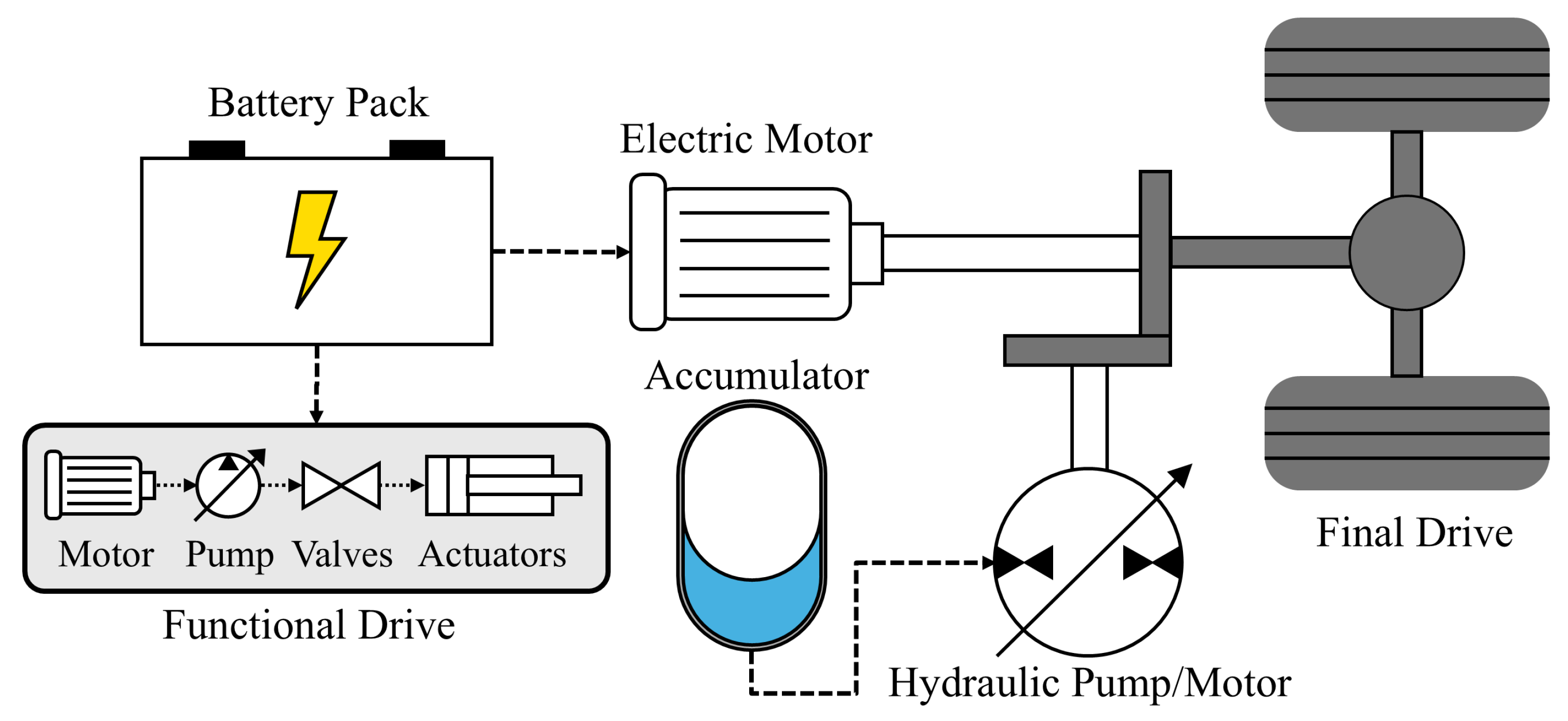
Figure 2.
Wheel loaders available to develop the input duty cycle including: (a) AHMCT ER-12 wheel loader and (b) Algoryx digital-twin simulation.
Figure 2.
Wheel loaders available to develop the input duty cycle including: (a) AHMCT ER-12 wheel loader and (b) Algoryx digital-twin simulation.
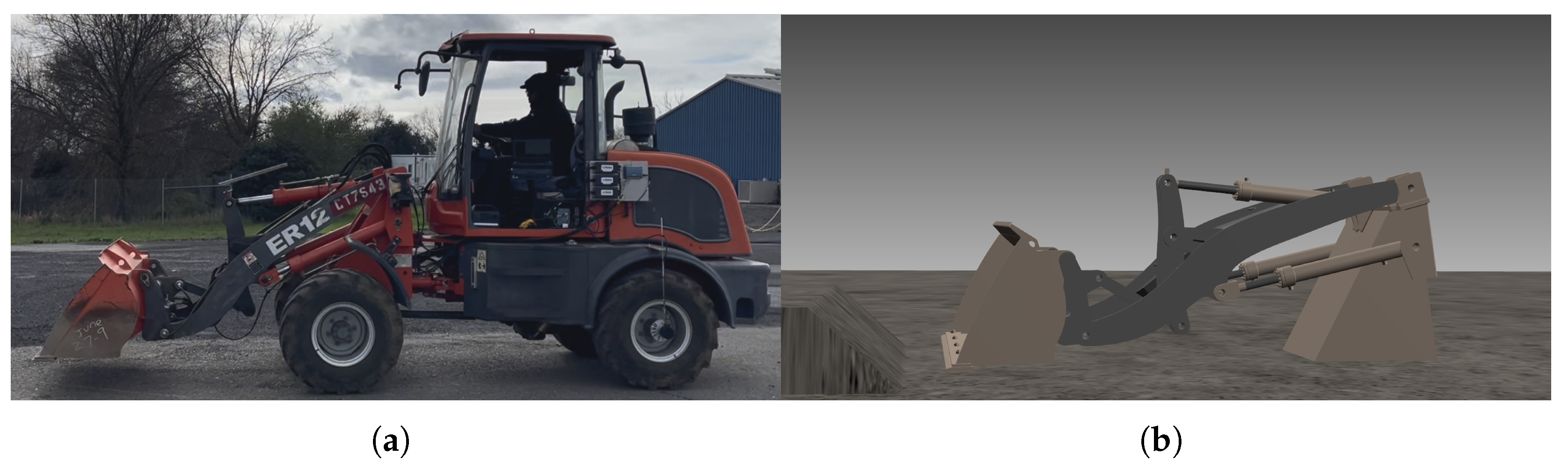
Figure 3.
Vehicle model inputs for 10 cycles which include: (a) the vehicle position, (b) the thrust force from the bucket contacting the material pile, and (c) the soil mass in the bucket. The vehicle dynamics convert these values into the powertrain model inputs of (d) the total torque required from the powertrain, (e) the rotational speed of the motors, and (f) the auxiliary power to lift and tilt the bucket.
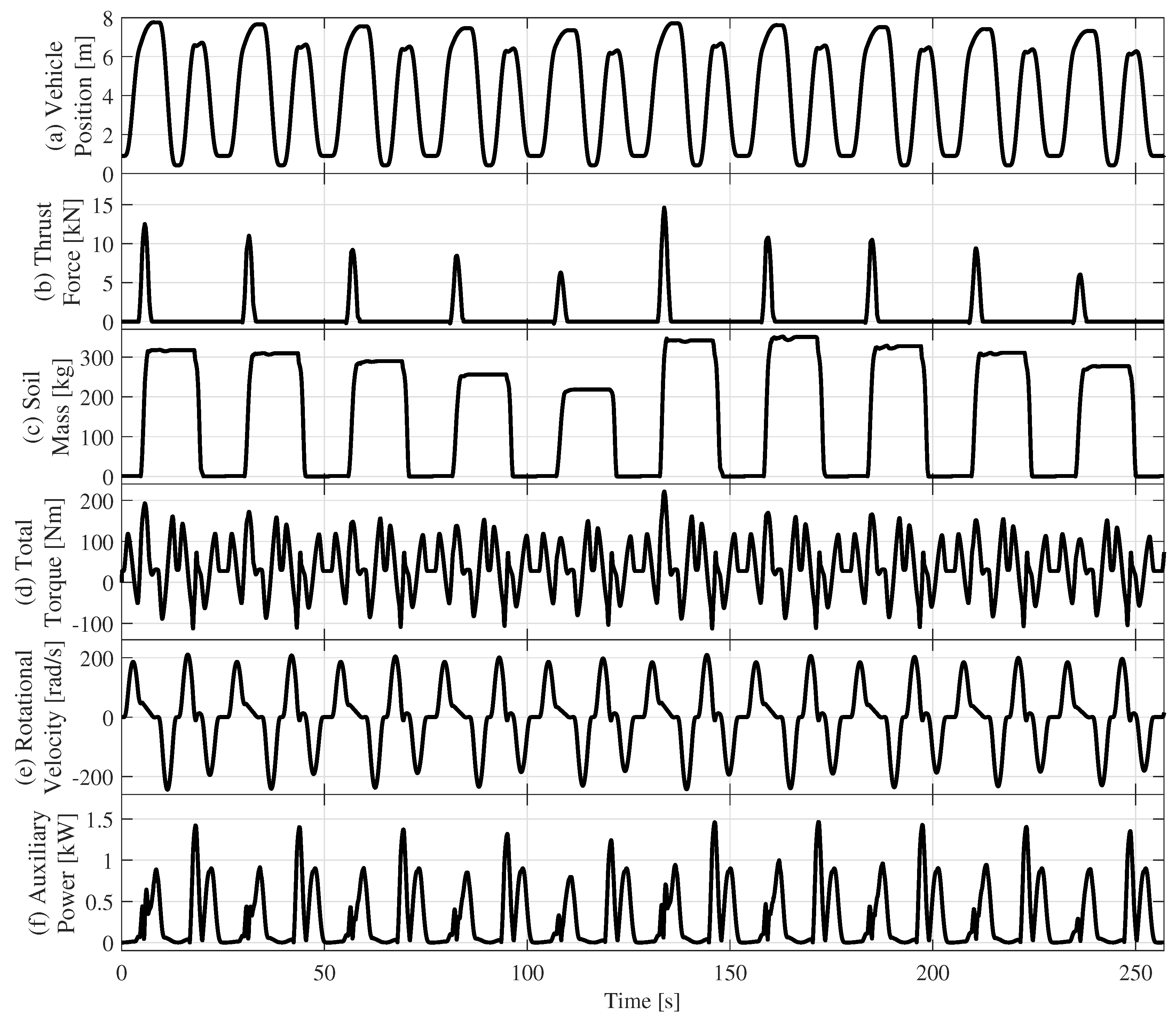
Figure 4.
Battery electrical model parameters developed from experiments on a 25 Ah LFP cell including: (a) open circuit voltage, (b) internal resistance, and (c) the resistance and (d) capacitance of the RC element as a function of the cell state of charge (SOC).
Figure 4.
Battery electrical model parameters developed from experiments on a 25 Ah LFP cell including: (a) open circuit voltage, (b) internal resistance, and (c) the resistance and (d) capacitance of the RC element as a function of the cell state of charge (SOC).
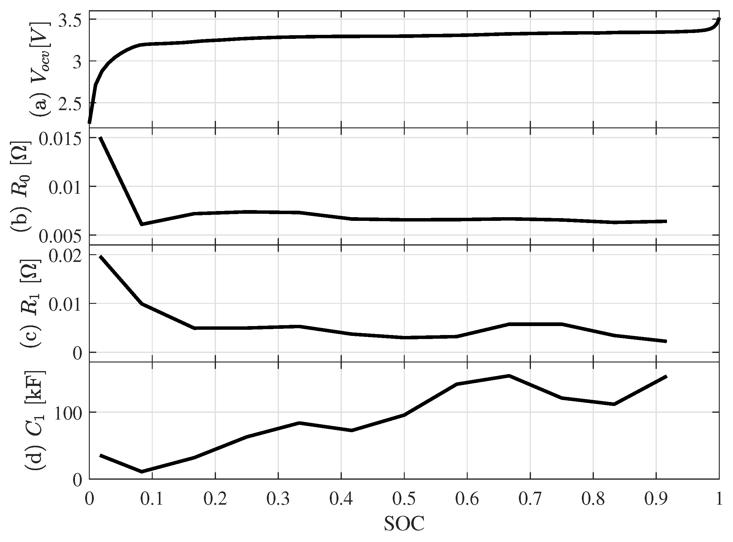
Figure 5.
Electric motor powerloss function model fit.
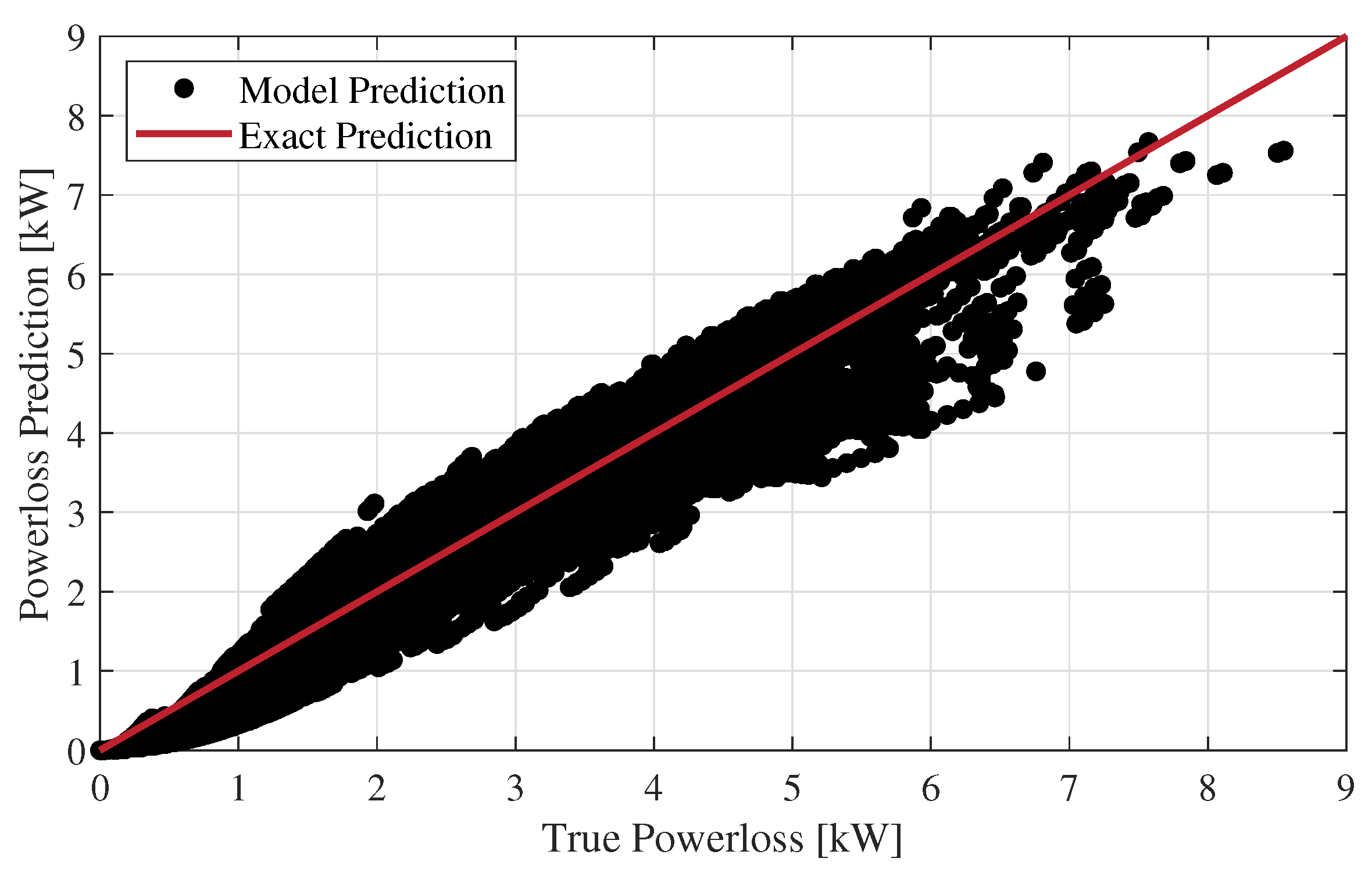
Figure 6.
Model validation results for one cycle described by: (a) the vehicle position. The following states are displays for both the high-order model and the control-oriented model: (b) battery SOC, (c) accumulator SOP, (d) battery power, (e) accumulator power, and (f) battery SOH.
Figure 6.
Model validation results for one cycle described by: (a) the vehicle position. The following states are displays for both the high-order model and the control-oriented model: (b) battery SOC, (c) accumulator SOP, (d) battery power, (e) accumulator power, and (f) battery SOH.
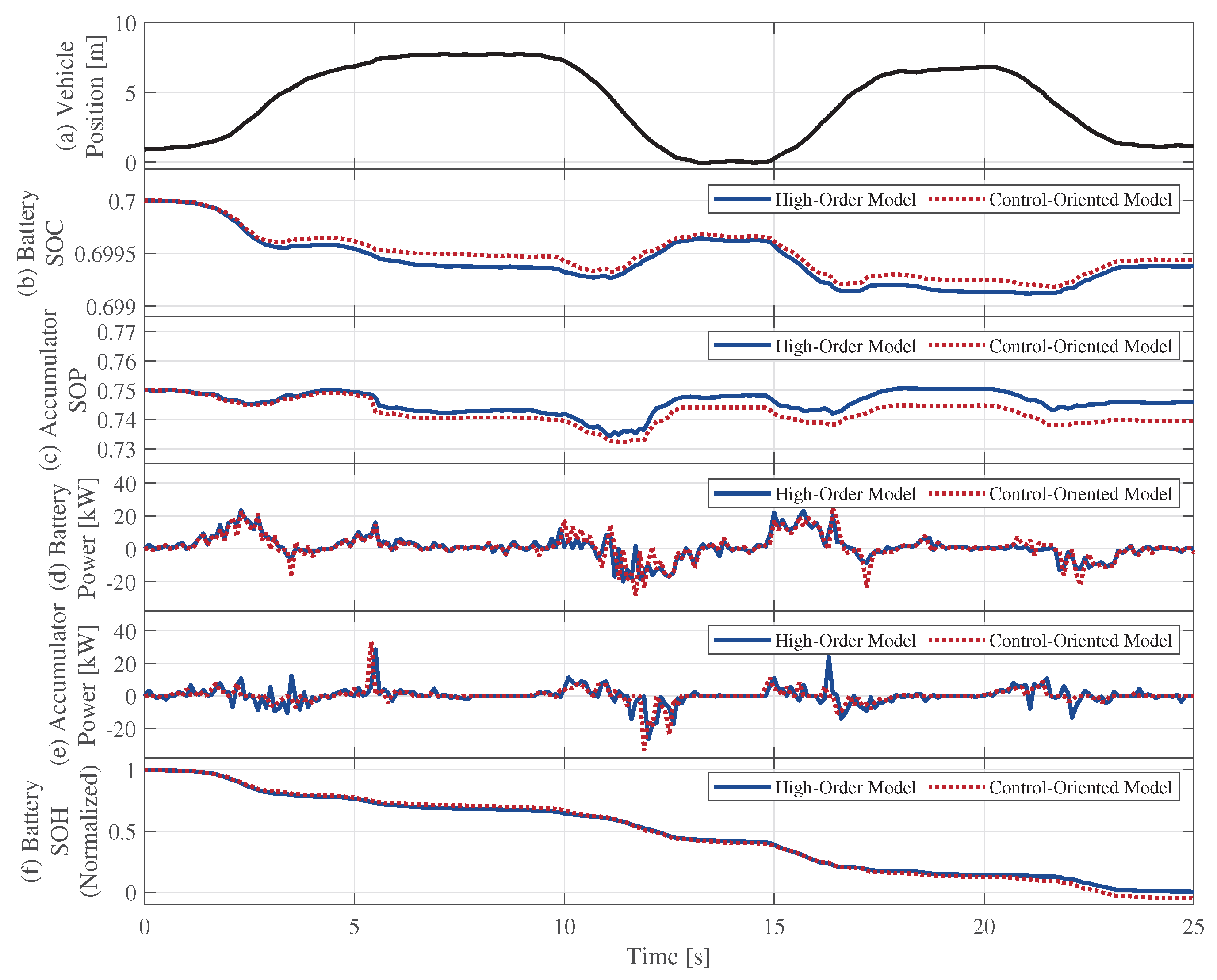
Figure 7.
Flow chart of Rule-Based energy management strategy.
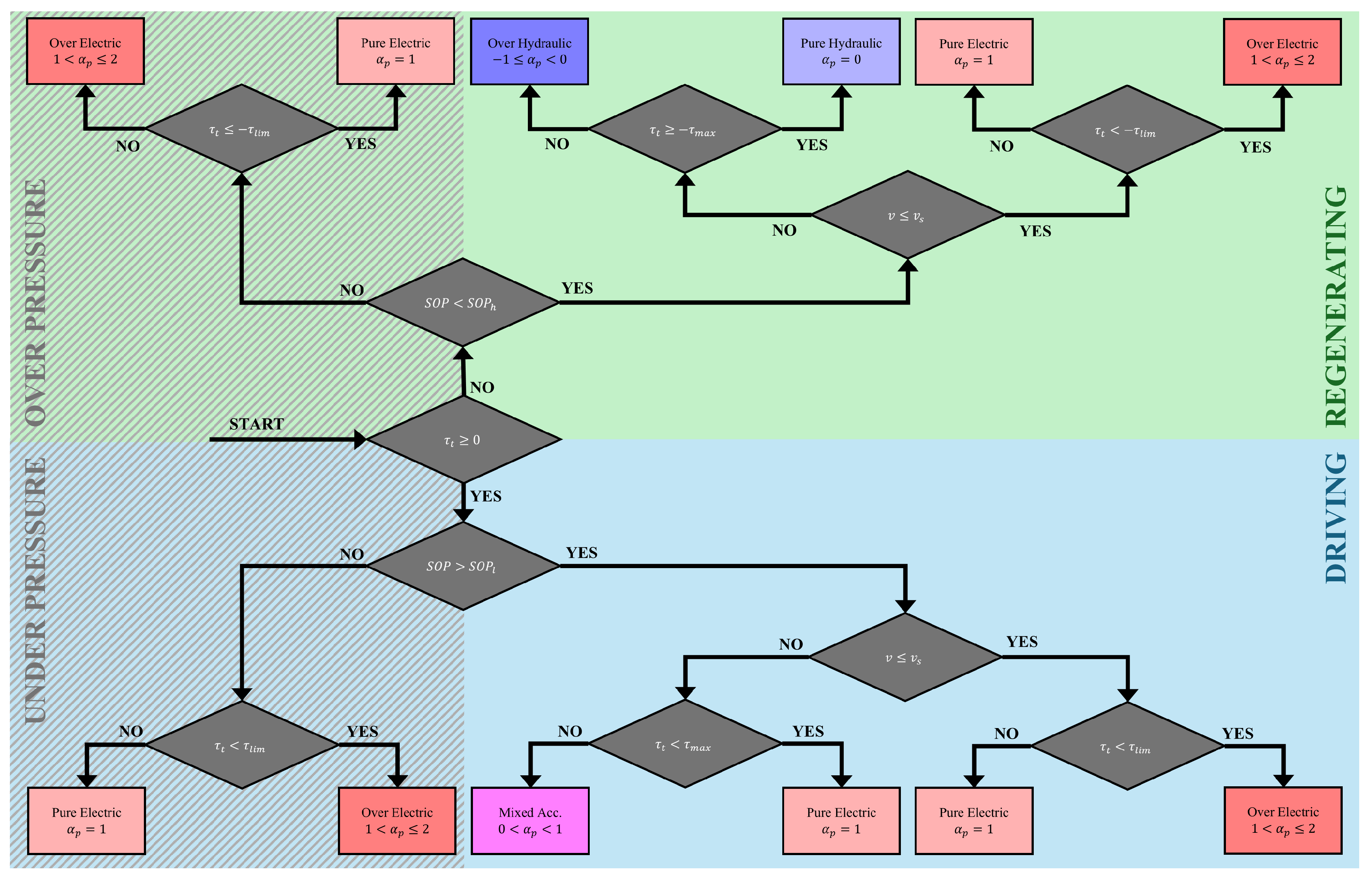
Figure 8.
The values of: (a) vehicle position, (b) motor angular velocity, and (c) total required torque, as well as the resulting control input of power-split ratio for one cycle of Rule-Based operation.
Figure 8.
The values of: (a) vehicle position, (b) motor angular velocity, and (c) total required torque, as well as the resulting control input of power-split ratio for one cycle of Rule-Based operation.
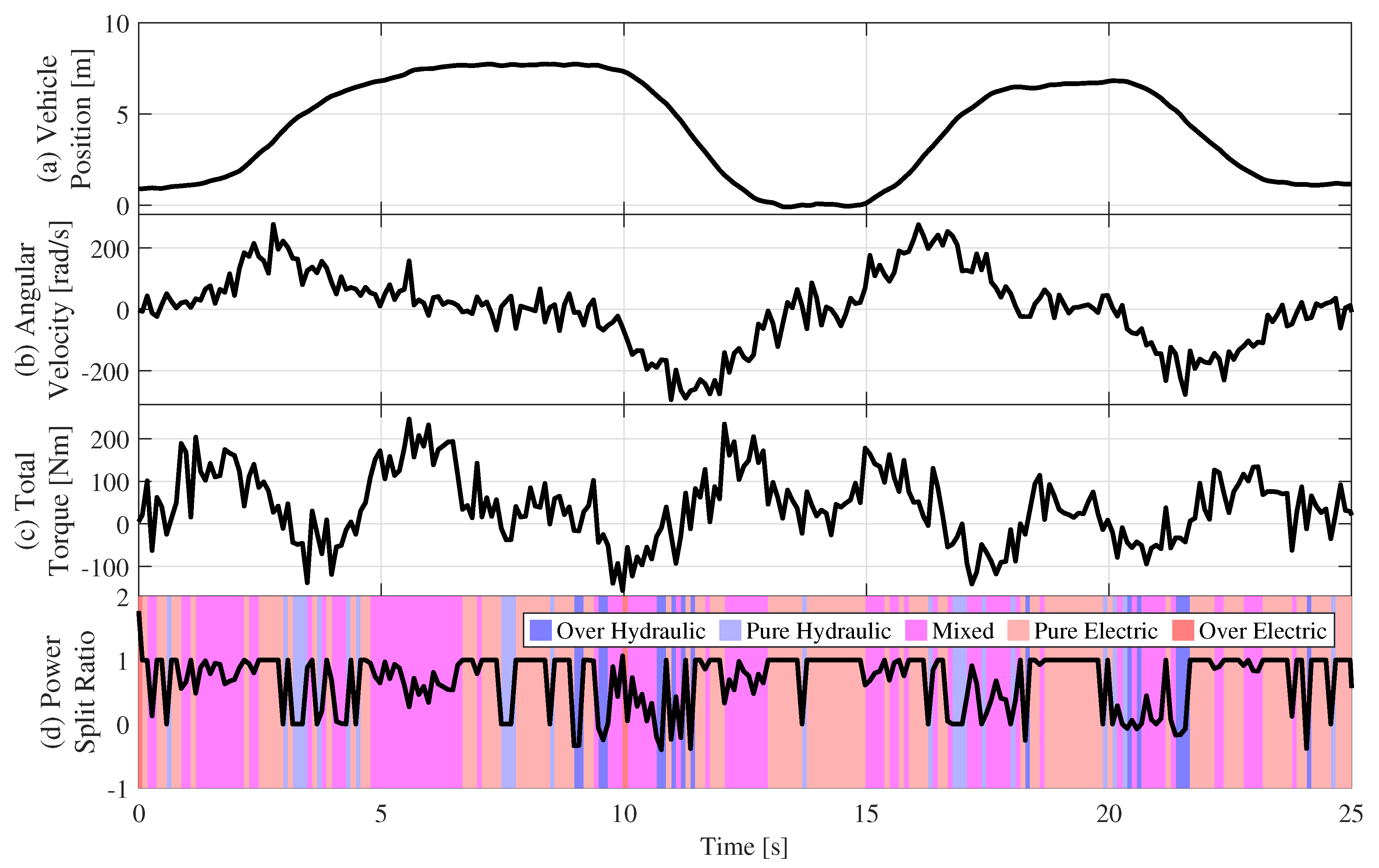
Figure 9.
One cycle of the actual versus predicted exogenous inputs with prediction having 20% error in: (a) the angular velocity of the motors, (b) the total torque required by the powertrain, and (c) the auxiliary power from the working hydraulics.
Figure 9.
One cycle of the actual versus predicted exogenous inputs with prediction having 20% error in: (a) the angular velocity of the motors, (b) the total torque required by the powertrain, and (c) the auxiliary power from the working hydraulics.
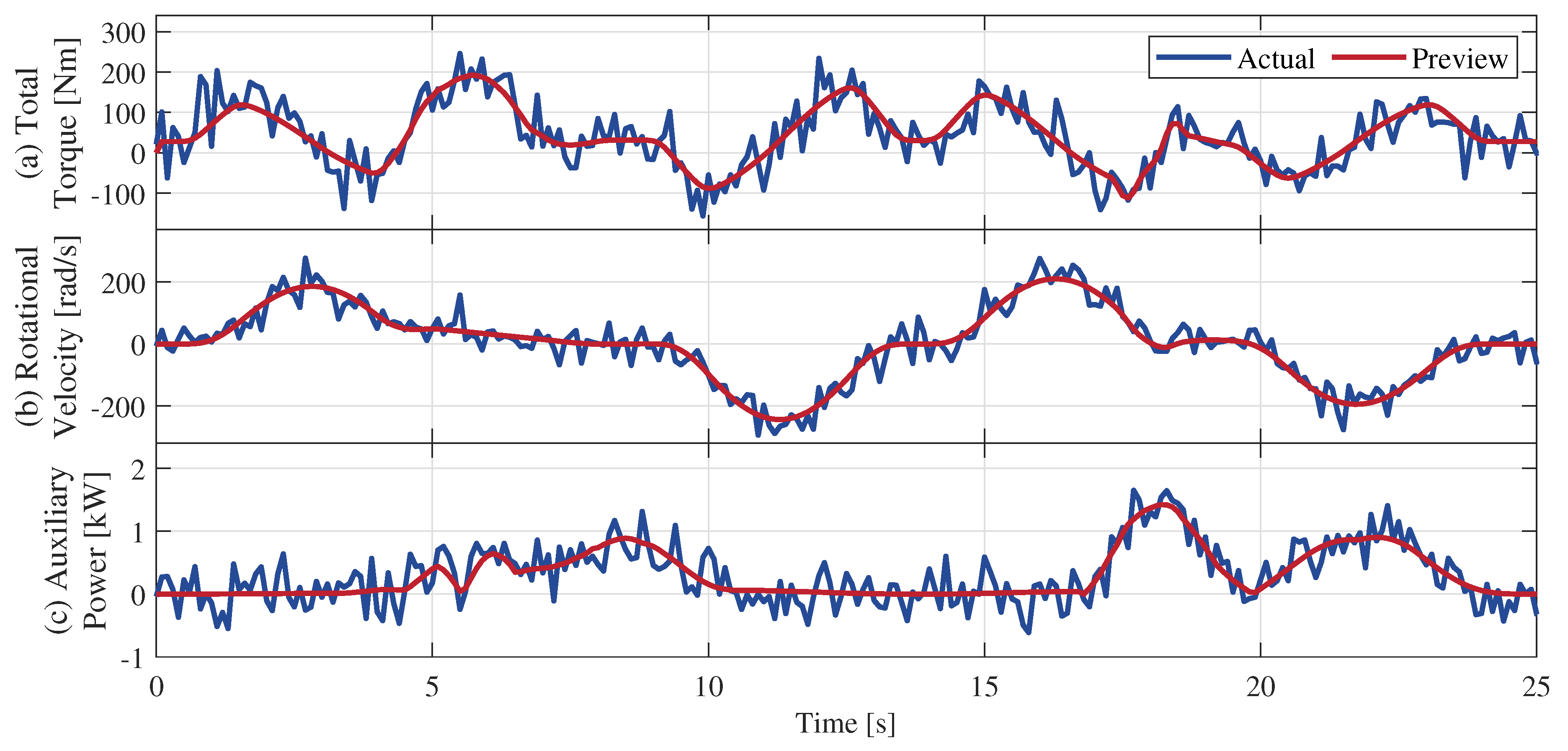
Figure 10.
Hardware-in-the-Loop test platform.
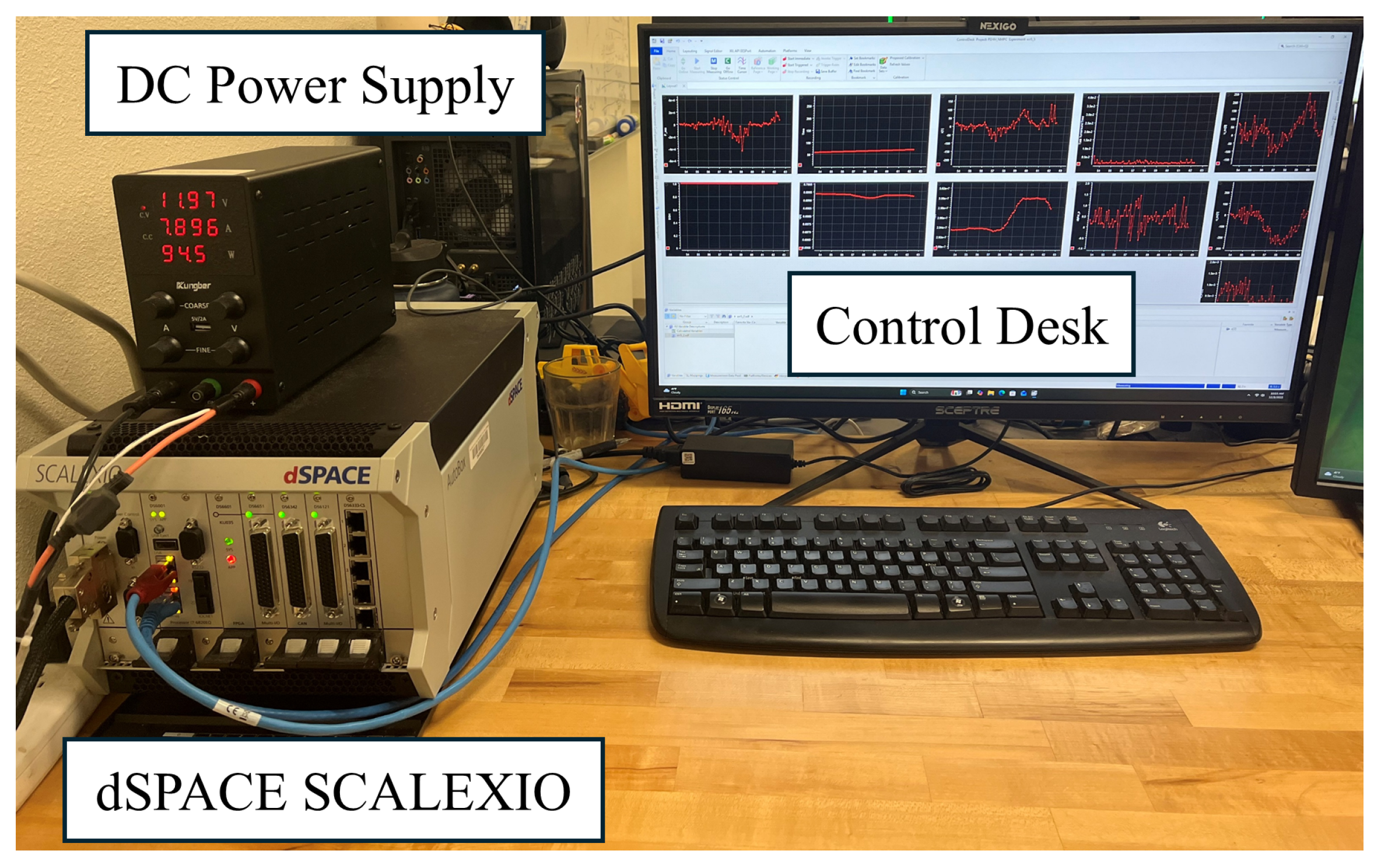
Figure 11.
Results for 10 cycles with inputs of: (a) the wheel loader position, (b) the motor angular velocity, and (c) the total torque required. The resulting (d) power-split ratio, (e) battery SOC, and (f) accumulator SOP are shown for 3 controllers: the Rule-Based energy management, NMPC with exact prediction, and NMPC with 20% prediction error.
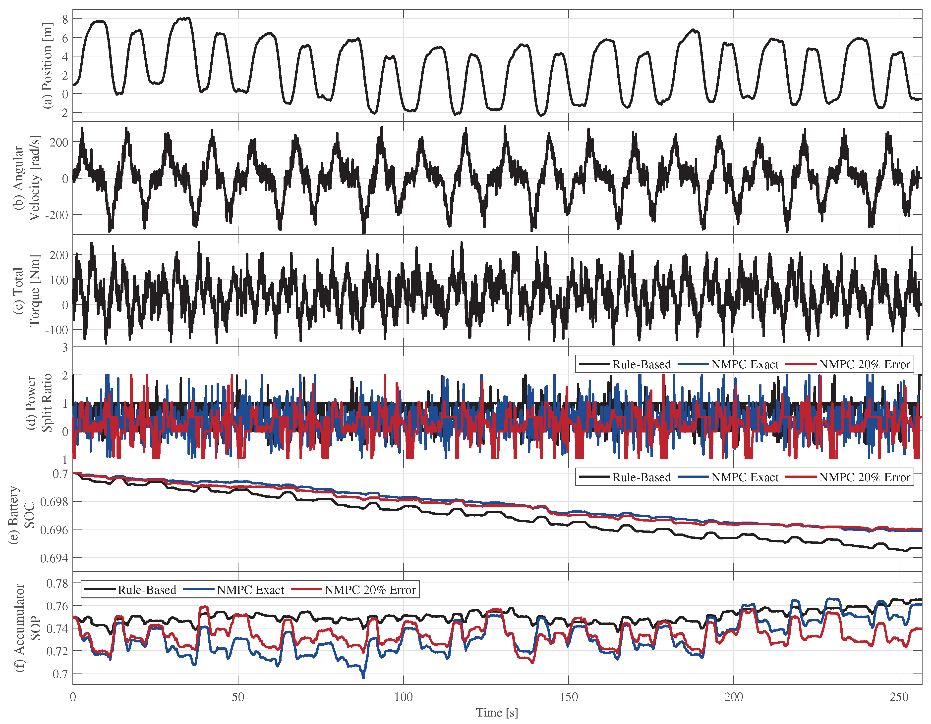
Figure 12.
Normalized SOH for Rule-Based and NMPC EMS with various levels of prediction error.
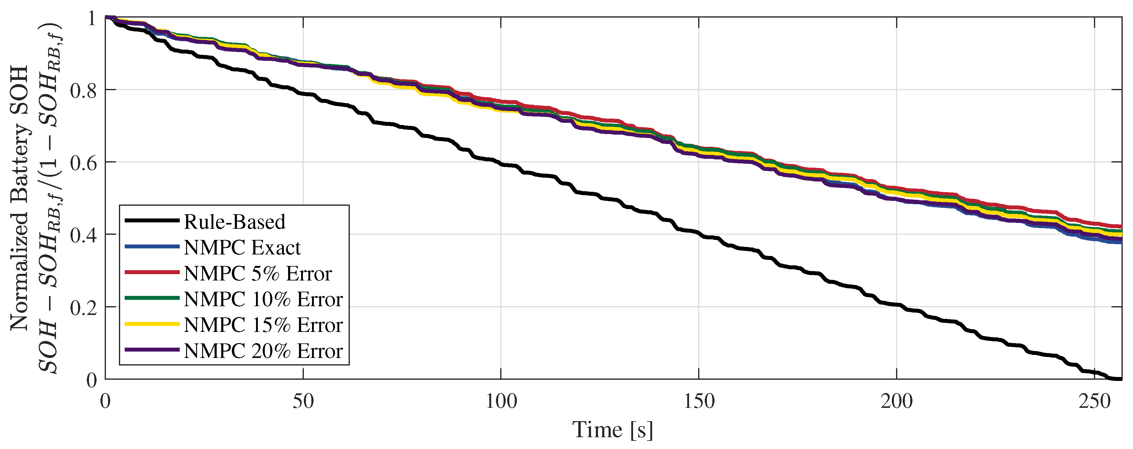
Figure 13.
Energy usage for Rule-Based and NMPC EMS with various levels of prediction error.
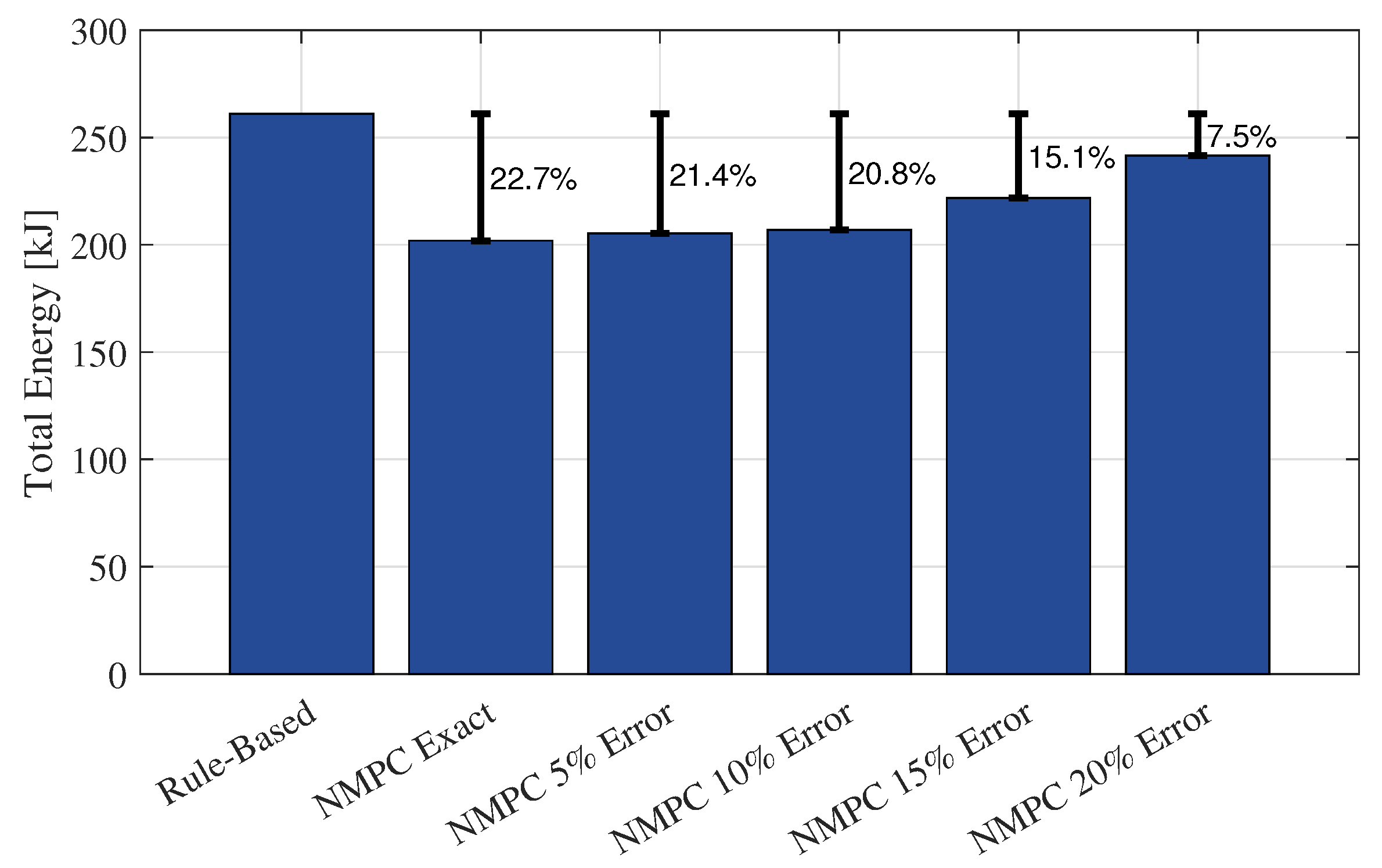
Figure 14.
Computation time for NMPC with various levels of prediction error.
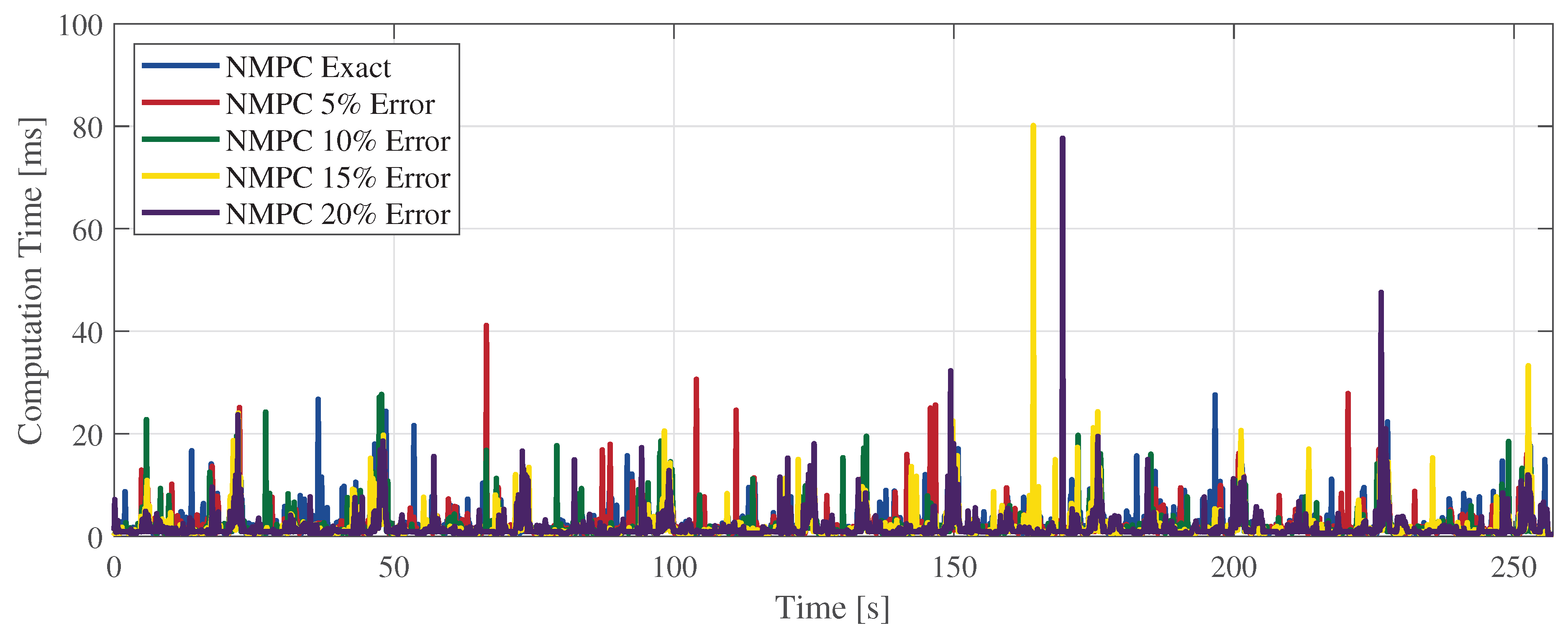

Table 1.
Electric motor powerloss function coefficients.
| Coefficient | ||||||
|---|---|---|---|---|---|---|
| Value | 6.21E-3 | 7.65E-9 | -3.36E-6 | -1.52E-2 | 9.07E-4 | 3.87E-4 |
Table 2.
Hydraulic motor torque loss and volumetric leakage functions coefficients.
| Coefficient | ||||||||
|---|---|---|---|---|---|---|---|---|
| Value | -0.290 | 3.42E-2 | 5.47E-9 | -8.96E-10 | 3.52E-3 | 738E-4 | -1.79E-9 | -6.44E-11 |
Table 3.
Control-oriented parallel electric-hydraulic hybrid powertrain model constant parameters.
| Variable | Description | Value | Units |
|---|---|---|---|
| Vehicle Model | |||
| Base Vehicle Mass | 3356 | kg | |
| Wheel Radius | 0.4 | m | |
| Final Drive Ratio | 30.39 | - | |
| Rolling Resistance Coefficient | 0.06 | - | |
| Traction Efficiency | 0.94 | - | |
| Electric Subsystem | |||
| Motor Time Constant | 50 | ms | |
| Battery Cells in Parallel | 3 | - | |
| Battery Cells in Series | 61 | - | |
| Battery Cell Capacity | 25 | Ah | |
| Battery Internal Resistance | 7.81E-3 | ||
| Battery RC Resistance | 6.19E-3 | ||
| Battery RC Capacitance | 7.84E3 | F | |
| Hydraulic Subsystem | |||
| Pump/Motor Volumetric Displacement | 131.44 | cc/rev | |
| Accumulator Volume | 100 | L | |
| Maximum Accumulator Pressure | 35 | MPa | |
| Minimum Accumulator Pressure | 15 | MPa | |
| Pre-Charge Pressure | 15 | MPa | |
| Nominal Accumulator SOP | 0.75 | - | |
Table 4.
Rule-Based energy management parameters.
| Parameter | |||||
|---|---|---|---|---|---|
| Value | 0.85 | 0.65 | 0.5 | 100 | 50 |
| Units | - | - | m/s | Nm | Nm |
Table 5.
Hardware-in-the-loop test platform specifications.
| Component | Specifications |
|---|---|
| dSPACE SCALEXIO AutoBox DS6001 | i7-6820EQ |
| PC Interface | i9-14900F |
Table 6.
NMPC computation time statistics for various levels of preview error.
| Error Level | 0% | 5% | 10% | 15% | 20% |
|---|---|---|---|---|---|
| Min time [ms] | 0.371 | 0.371 | 0.372 | 0.371 | 0.371 |
| Max time [ms] | 27.58 | 41.12 | 27.67 | 80.12 | 77.66 |
| Avg time [ms] | 2.014 | 1.836 | 1.747 | 1.684 | 1.707 |
| Std time [ms] | 2.496 | 2.612 | 2.517 | 2.981 | 2.871 |
Disclaimer/Publisher’s Note: The statements, opinions and data contained in all publications are solely those of the individual author(s) and contributor(s) and not of MDPI and/or the editor(s). MDPI and/or the editor(s) disclaim responsibility for any injury to people or property resulting from any ideas, methods, instructions or products referred to in the content. |
© 2026 by the authors. Licensee MDPI, Basel, Switzerland. This article is an open access article distributed under the terms and conditions of the Creative Commons Attribution (CC BY) license (http://creativecommons.org/licenses/by/4.0/).
Copyright: This open access article is published under a Creative Commons CC BY 4.0 license, which permit the free download, distribution, and reuse, provided that the author and preprint are cited in any reuse.


