
Submitted:
29 January 2026
Posted:
30 January 2026
You are already at the latest version
Abstract
Background: Sepsis remains a leading cause of mortality in Intensive Care Units (ICUs) worldwide. Machine learning models for clinical prediction must be accurate, fair, transparent, and reliable to ensure that physicians feel confident in their decision-making process. Methods: We used the MIMIC-IV, version 3.1, database to evaluate several machine learning architectures, including Logistic Regression, XGBoost, LightGBM, LSTM (Long Short-Term Memory) networks and Transformer models. We predicted three main clinical targets: hospital mortality, length of stay, and septic shock onset. Model interpretability was assessed using Shapley Additive Explanations (SHAP). Results: The XGBoost model demonstrated superior performance in prediction tasks, particularly for hospital mortality (AUROC 0.874), outperforming traditional LSTM networks, transformers and linear baselines. Importance analysis of the variables confirmed the clinical relevance of the model. Conclusions: While XGBoost and ensemble algorithms demonstrate superior predictive power for sepsis prognosis, their clinical adoption necessitates robust explainability mechanisms to gain the doctors trust.
Keywords:
sepsis
; machine learning
; artificial intelligence
; responsible artificial intelligence
; mimic-iv
; intensive care unit
1. Introduction
According to the World Health Organization [1], sepsis is one of the leading causes of death worldwide, with 48.9 million cases and 11 million deaths in 2020 alone, representing 20% of all deaths worldwide.
In addition to the high mortality rate, sepsis treatment is excessively expensive, given the occupancy of intensive care unit (ICU) beds, long hospital stays, need for constant monitoring, and complex treatments. The average hospital-wide cost of sepsis was estimated to be more than US$32,000 per patient in high-income countries [2].
Sepsis-3, since the 2016 consensus conference, has been defined as an infectious episode leading to life-threatening organ dysfunction caused by an inadequate host response to infection [3].
Although physicians have an abundance of information about patients in the ICU for the treatment of sepsis, such as laboratory results, imaging studies, and clinical documentation, this cognitive overload can often hinder the identification of relevant patterns and the decision-making process [4].
Artificial Intelligence (AI) and Machine Learning (ML) have demonstrated great potential for predicting, diagnosing, and providing individualized treatment for sepsis. In diagnosis, AI has shown advantages over traditional sepsis classification systems, such as the Systemic Inflammatory Response Syndrome (SIRS), Sequential Organ Failure Score (SOFA), and quick SOFA (qSOFA), identifying sepsis several hours in advance [5,6]. Early detection allows clinicians to intervene faster, increasing the chances of successful treatment [7].
However, the "black-box" nature of advanced Machine Learning Models (MLMs) poses a significant barrier to clinical adoption [8]. Machine learning models for clinical prediction must be accurate, fair, transparent, and reliable [9] so that physicians feel confident in their decision-making process [10]. Responsible AI practices are crucial for predicting sepsis, a disease with high mortality rates and length of hospital stay [11,12,13,14,15].
This study explored the prediction of mortality, length of stay, and septic shock in patients with sepsis using Artificial Intelligence algorithms, respecting the following principles regarding responsible AI:
- Transparent and Explicable: Can physicians understand why a prediction was made?
- Trust: Are the predictions reliable and free of data leaks?
- Fairness: Do the models perform equally well in all patient subgroups?
- Privacy: Are patient data handled responsibly?
In this study, we used a sepsis-3 cohort extracted from MIMIC-IV [16], version 3.1 [17], containing 35.215 ICU admissions that met the criteria for Sepsis-3, with selected and time-aligned characteristics, including vital signs, laboratory test results, and therapeutic interventions, such as vasopressors, intravenous fluids, and antibiotics.
2. Materials and Methods
This study used Machine Learning (ML) for the prediction of mortality, length of stay, and septic shock in patients with sepsis, respecting the principles of Responsible AI, and was developed following the Transparent Reporting of a Multivariable Prediction Model for Individual Prognosis or Diagnosis, with Artificial Intelligence (TRIPOD-AI) reporting guidelines [18], aligning with the standards that balance innovation with clinical responsibility suggested in recent editorials [19].
This study was developed based on a public benchmark on Sepsis-3 using the MIMIC-IV database, version 3.1, which is a large, freely available database comprising de-identified health-related data associated with patients who stayed in the critical care units of the Beth Israel Deaconess Medical Center [20].
2.1. Data Source
The MIMIC-IV database version 3.1, officially released in October 2024, was used. It contains hospitalization data for 364,627 unique patients between 2008 and 2022. This database aligns with ethical and safety principles, as its structure and governance incorporate many ethical pillars required for the development of safe healthcare systems.
The privacy and security principles are guaranteed when providing an anonymized database, meaning that personal identifiers of patients and healthcare professionals have been removed or altered to protect their identity, in accordance with the Health Insurance Portability and Accountability Act (HIPAA). Unlike open databases, access to MIMIC-IV requires researchers to complete research ethics training provided by the PhysioNet platform and sign a Data Use Agreement (DUA). The PhysioNet platform is managed by members of the MIT Laboratory for Computational Physiology [17,21].
MIMIC-IV promotes the principle of transparency by making the code for the data processing scripts (SQL and Python) available on the GitHub platform, allowing the scientific community to audit and reproduce the results. Furthermore, the community is encouraged to contribute to the project, either by proposing improvements or reporting possible errors.
2.2. Cohort Selection
This section describes how the cohort was generated according to the authors. The cohort process was based on methodologies from prior sepsis studies [22] that preserved the temporal structure of the clinical trajectories. The data were extracted and grouped into categories such as (1) demographics, such as age, sex, and gender; (2) clinical measurements, such as laboratory tests and vital signs; and (3) clinical interventions, such as vasopressors, fluids, and mechanical ventilation.
To identify suspected infection, the Sepsis-3 definition was used [3], using either antibiotic administration records or positive microbiological cultures as potential infection triggers, the earliest time point where a patient’s SOFA score increased by two or more points from baseline. A 24-hour window before and 72 hours after the onset of sepsis was defined. This window aims to capture early detection signs up to the acute phase of infection. The clinical measurements in this window were standardized, and outliers were removed. The data were regrouped at 4-hour intervals. The mean was computed when multiple values were present within an interval.
The missing data shortage is addressed through a layered imputation strategy inspired [22]. Linear interpolation was used for variables with low amounts of missing data (<5%) to preserve local temporal trends, and K-nearest neighbors (KNN) imputation [23] was applied for moderate amounts of missing data to explore correlations between similar patient profiles in the multivariate feature space.
Variables with more than 80% of the data missing were removed to avoid the risk of introducing bias when performing imputation. Some variables are estimated based on clinical rules, such as FiO2, which is derived from the oxygen flow rate and device type, and the Glasgow Coma Scale (GCS), which is calculated from the RASS Score [24]. SOFA, NEWS, and SIRS scores were calculated from the cleaned data.
Four types of central interventions for the treatment of sepsis were extracted: (1) mechanical ventilation (mode and parameters), (2) antibiotics (timing and number of unique agents), (3) fluid resuscitation (standardized to 0.9% NaCl equivalent volume), and (4) vasopressors (converted to norepinephrine-equivalent dosage). Every 4h, cumulative vasopressor levels, doses, and volumes were recorded. These variables allow us to observe not only the patient’s status but also the dynamics of the treatment.
Septic shock is defined using three conditions: (1) administration of at least 2000 mL of fluids in the prior 12 hours, (2) MAP < 65 mmHg despite fluid resuscitation, and (3) vasopressor requirement with lactate > 2 mmol/L [3,25].
Patients under 18 years of age, patients with insufficient data, and individuals who died shortly after admission to the ICU were excluded, indicating that they did not have time for adequate treatment.
2.3. Data Preprocessing
Clinical data were extracted and processed into time-series formats using the reproducible pipeline established by [20]. After review by clinicians, we calculated and added the NEWS Score [26] to this pipeline, an important score to help identify sepsis early [27].
Table 1 lists the predictor variables used in the tasks, excluding identifiers and target variables such as mortality, length of stay (LOS), and septic shock. The predictor variables were grouped into the following categories: demographic data, vital signs, laboratory tests, hematological tests, arterial blood gas analysis, ventilation and oxygenation, liver function, clinical scores, and fluid administration.
In total, the cohort contained 78 predictor variables, some of which were derived from other information, such as score variables like NEWS, and some variables could be considered redundant, such as temp_C (temperature Celsius) and temp_F (temperature Fahrenheit). The complete list in alphabetical order is presented in Table A1.
Records with outliers were excluded. The initial cohort contained 36,613 records identified as sepsis. Within this set, 13 records were excluded due to extreme urine values, exceeding 12.000 ml within a 4-hour period, possibly due to typing or sensor errors.
Twelve records of patients who received over 10.000 ml of fluids within a 4-hour period were also excluded. A total of 870 records were excluded due to premature death occurring within less than 24h after ICU admission, as these patients were considered to have advanced sepsis, and the model would not be able to systematically track the progression of the condition, potentially introducing future bias.
A further 503 records were excluded because they did not have a SOFA score greater than 2 throughout their hospital stay, failing to meet the sepsis-3 criteria. Therefore, 1.374 records were excluded, resulting in a final model with 35.215 records.
2.4. Data Statistics
Table 2 presents the cohort characteristis. The average age of the patients is 65 years, with a standard deviation of 16.3 years plus or minus, with 38.1% between 41 and 65 years old. There was a relative predominance of male patients (approximately 55%). The median Charlson comorbidity index of 5.0 suggests a considerable burden of comorbidities in this population. According to the BMI criteria, more than 60% of the patients were overweight or obese.
The Mortality rate during hospitalization was 14.5%. However, mortality within 90 days was 25.5%, reflecting the difference between patients who were discharged alive but subsequently died. The average Length of ICU Stay (LOS) was 5.1 days, with a standard deviation of 7.1 days. Because the standard deviation (7.1) is greater than the mean (5.1), this confirms that the distribution is very asymmetrical (some patients stay for a long time, pulling the mean upwards). The median (2.65 [1.37-5.73]) was the best measure of central tendency for the LOS.
The mean SOFA Score of 5.5 (± 2.8) reflects substantial organ dysfunction, typical of patients who meet the Sepsis-3 criteria, indicating a significant but not extreme risk of in-hospital mortality. The mean NEWS score of 6.06 (± 2.57) indicates a medium-to-intermediate risk of clinical deterioration in a patient. This score indicates that the patient’s vital signs vary significantly from normal levels and require frequent monitoring.
The mean values of the Glasgow Coma Scale (GCS) and RASS scores were consistent with septic conditions, indicating that these patients frequently have altered mental status or are sedated, and may also be drowsy. Most patients were treated with antibiotics (66.3%), while 35.1% required mechanical ventilation and 16.9% used vasopressors.
Table 3 presents the baseline characteristics of the survivors and non-survivors. Most variables showed statistically significant differences (). Non-survivors were older and had a higher burden of comorbidities, as shown by the Charlson Index. Admission severity scores, including SOFA and NEWS scores, were significantly elevated in this group. Laboratory markers also confirmed the presence of greater organ dysfunction. In contrast, sex, SIRS score, and temperature did not differ significantly between outcomes.
2.5. Machine Learning Models
This study evaluated predictive models across three critical clinical tasks in the context of sepsis: mortality prediction, Length of Stay(LOS), and septic shock. These tasks were grouped into two categories based on their temporal structures:
- 1.
- Static Prediction: for mortatility and LOS, the models use only the first 24 hours after sepsis detection. Clinical data were aggregated into 4-hour time steps, and six time steps (equivalent to 24 hours) of data were used to make predictions. We represent the time steps for , where N represents the time steps; for example, represents the more recent moment and represents five time steps before (between 20h and 24h).
- 2.
- Dynamic Prediction with sliding window: for the septic shock, the model take the last 24h (window_size = 6) an try to predict if the event (sepsis shock) will occur in the next 24h (prediction_horizon=6). Therefore, the model learns to predict the event at any point during the stay by looking at the recent 24-hour history.
Table 4 summarizes the prediction tasks, modeling setup, and evaluation metrics. Mortality and septic shock prediction are defined as binary classification problems and LOS as a regression. We standardized the metrics across tasks to enable consistent and fair comparisons between the models.
For the Mortality and septic shock tasks, we used binary classification to predict the probability of event occurrence. To evaluate these models, we employed the Area Under the Receiver Operating Characteristic curve (AUROC) and the Area Under the Precision-Recall Curve (AUPRC). While AUROC measures the overall discriminative power, AUPRC is particularly informative in clinical datasets, where class imbalances are prevalent. The general performance was also measured using accuracy.
where , , , and represent true positives, true negatives, false positives, and false negatives, respectively.
The Length of Stay (LOS) task is addressed as a regression problem. The performance was quantified using the Mean Absolute Error (MAE), which provides a direct interpretation of the average error magnitude, and the Root Mean Squared Error (RMSE), which is more sensitive to large outliers:
where is the actual value, is the predicted value, and n is the total number of observations.
We evaluated a diverse set of algorithms to capture both linear and non-linear patterns. The specific configurations of each algorithm were as follows:
- Linear Models: For Classification tasks (Mortality, Septic Shock), Logistic Regression is used. For Regression tasks, LOS, Ridge Regression were used, which is a Linear Regression with L2 regularization (alpha=1.0) to mitigate overfitting in the high-dimensional feature space.
- Random Forest: Build many Decision Trees () with fully grown depth and a minimum sample split of 2 [28].
- XGBoost: Gradient boosting configured with 100 estimators, a maximum tree depth of 6, and a learning rate of 0.1 [29].
- LightGBM: Optimized with 100 boosting iterations, a maximum depth of 6, and a learning rate of 0.1 [30].
- Long Short-Term Memory (LSTM): Recurrent Neural Network (RNN) architecture designed to capture long-term dependencies in time-series data, used with 2 stacked layers, 64 hidden units per layer, and a dropout rate of 0.1. The model was trained using an Adam learning rate of 0.001 [31].
- Transformer: Neural Network (NN) with Attention-based model with 2 encoder layers, 8 attention heads, a feed-forward dimension of 256, and a dropout rate of 0.1. The model was trained using a learning rate of 0.001.
All experiments adhered to reproducibility standards. The data were partitioned into 80% training and 20% validation sets using a stratified split at the patient level. A fixed random seed (seed=42) was applied to all data splits to ensure consistent reproducibility across all models. Experiments were implemented in Python, utilizing Pandas and NumPy for data manipulation, Scikit-learn for linear models, Random Forest, and evaluation metrics, PyTorch for deep learning architectures, and the official XGBoost and LightGBM libraries for gradient boosting.
SHAP (SHapley Additive exPlanations) analysis was employed to ensure the model’s transparency and clinical interpretability [32]. SHAP analysis provides three levels of explainability through three graphics: (1) overall importance of the feature (summary bar), (2) distribution of the feature’s impact among patients (beeswarm), and (3) individual explanations of the predictions (waterfall plot). This multi-level transparency meets the key requirements of responsible AI in healthcare applications.
3. Tasks and Results
Three types of tasks were prepared from the cohort: mortality, length of stay, and septic shock. This section describes the tasks, the test results and which features were most important to the results.
3.1. Mortality Task
The predictive efficacy was quantified using a combination of AUROC, AUPRC, and Accuracy. Given the prevalence of class imbalance in the MIMIC-IV dataset, where septic events are significantly less frequent than non-events, the AUPRC serves as a critical metric for evaluating the trade-off between sensitivity and positive predictive value [33]. This was complemented by the AUROC to determine the global discriminative capacity and accuracy to assess the total proportion of correct classifications, ensuring a comprehensive validation of the model’s clinical utility. Table 5 presents the results of the tests for all algorithms.
Comparative analysis of mortality prediction revealed that gradient-boosted decision trees (GBDTs) outperformed both traditional linear models and complex deep learning architectures. XGBoost achieved the highest performance across all metrics, with an AUROC of 0.874 and AUPRC of 0.606. XGBoost demonstrated superior precision in identifying the positive class, as evidenced by its higher AUPRC.
Despite having the same AUROC as LightGBM, XGBoost performed better in terms of AUPRC, indicating that it made fewer errors in predicting death (fewer false-positives in the minority class).
Deep learning models, such as transformers and LSTM, achieve good results but are often outperformed by tree-based models on tabular data [34,35]. Unlike studies utilizing unstructured clinical text [36], our structured approach facilitates integration into standard workflows.
Figure 1 presents the confusion matrices for the four best algorithms in this task. The layout follows the Scikit-Learn Python library standard, where class 0 (negative/survivor) is presented in the first row/column and class 1 (positive/death) in the second.
The confusion matrix can be interpreted as follows:
- Upper left quadrant: True Negatives (TN), representing patients who survived (negative), and the model correctly predicted survival.
- Upper right quadrant: False Positives (FP), representing patients who survived (negative), but the model incorrectly predicted death (positive). This situation is a false alarm that can be ignored.
- Lower left quadrant: False Negatives (FN), representing patients who died (positive), but the model incorrectly predicted survival (negative). This is a critical error.
- Lower right quadrant: True Positives (TP), representing patients who died (positive), and the model correctly predicted death.
The main diagonal (TN and TP) contains the correct predictions (starting with ’True’). The secondary diagonal (FN and FP) contains incorrect predictions (starting with ’False’). The first and second rows represent surviving and deceased patients, respectively.
The random forest model (Figure 1(d)) exhibited highly conservative behavior; while it minimized the lowest false-positive count (85), it exhibited a clinically concerning rate of False Negatives (776), failing to identify a significant proportion of patients at high mortality risk. On the other hand, the Transformer, Figure 1(c), identified the highest number of True Positives (380), but it had a higher rate of false positives, which could contribute to excess alarms in a clinical setting.
The XGBoost (a) and LightGBM (b) models exhibited the most balanced diagnostic performances. In particular, XGBoost showed superior consistency. It demonstrated better control over false positives (161 against 177 for LightGBM) and achieved the highest overall discriminative ability, with AUROC = 0.874 and AUPRC = 0.606, respectively.
Figure 2 shows a summary bar for XGBoost mortality prediction. The top-15 predictors are displayed along with their relevance to the model. According to the XGBoost algorithm, the Oxygen Flow Device (serving as a proxy for respiratory severity and need for intervention), Charlson Comorbidity Index, Urea Nitrogen, and the Sofa Score were the main predictors of mortality.
On the predictor variables side, we have the measurement time, which was taken every 4 hours, as explained earlier. For the mortality prediction task, the first 24 hours were used to predict mortality. The interval T-0 represents the most recent measurements, taken 24 hours after sepsis identification, while T-1 refers to measurements within 20 hours of sepsis identification, and T-5 refers to measurements at the time of sepsis identification.
The SHAP beeswarm plot visualizes the global importance and directional effects of each feature. The variables were ranked vertically according to their overall influence on the models. The horizontal axis represents the SHAP value: positive deviations to the right of the vertical line indicate an increased probability, whereas negative values to the left of the vertical line suggest the opposite effect. The color gradients denote the original feature magnitudes: red for high values and blue for low values.
The SHAP analysis in Figure 3 reveals that the Oxygen Flow Device, Charlson Comorbidity Index and Urea Nitrogen are the top predictors of mortality, where high values (red points) correspond to positive SHAP values, indicating an increased risk. In contrast, the Glasgow Coma Scale (GCS) score and Urine Output (Uo) showed an inverse relationship: high values, red color, shift towards the negative SHAP region, and reduced risk of mortality. Low values (blue), representing reduced consciousness, were strongly associated with higher mortality.
The SHAP waterfall plot shows the decision-making process of the model for a single instance, visualizing how each feature changes the prediction from the population baseline expected value to the final individual probability. Features are displayed in descending order of impact, where red bars indicate factors that increase the probability model and blue bars represent factors that decrease the probability.
In the case represented by Figure 4, the model estimated a low mortality probability, represented by the vertical line and the function value , which was significantly lower than the baseline of .
Despite the presence of static risk factors, such as advanced age () and comorbidities (Charlson Comorbidity Index, ), the prediction was driven down by the dominant protective clinical indicators. Specifically, the absence of high-risk respiratory support requirements (Oxygen Flow Device, ), combined with timely antibiotic administration (Hours Since First Abx, ) and stable physiological parameters (News Score and Urea Nitrogen, each), effectively mitigated the risk, leading to a favorable survival prediction.
3.2. Length of ICU Stay Task
For the regression task of predicting Length of Stay (LOS), the results shown in Table 6 confirm the dominance of gradient boosting algorithms over deep learning architectures in tabular clinical data.
LightGBM achieved the best performance, registering the lowest errors across all metrics (RMSE: 4.801; MAE: 2.599), closely followed by XGBoost. This indicates that tree-based ensemble methods are more effective at capturing non-linear relationships and interactions between clinical variables in tabular data [34,35] than recurrent or attention-based networks.
Complex deep learning models, such as Transformers and LSTMs, performed worse in this regression task, resulting in higher error rates (RMSE of 5.486 and 5.049, respectively). Complexity is not always associated with high accuracy.
Clinically, the Mean Absolute Error (MAE) of approximately 2.6 days achieved by the LightGBM model represents a good parameter for resource planning, offering a reasonably accurate margin for bed management and discharge scheduling.
There are no confusion matrices for LOS because this is a regression task (we are predicting a continuous number of days, e.g., 2.5 days) and not a classification (yes/no) task.
Feature importance analysis for the Length of Stay (LOS) regression task, Figure 5 reveals that indicators of organ dysfunction and therapeutic intensity are the primary drivers of hospitalization duration. Length of stay (LOS) prediction is heavily influenced by dynamic physiological responses and resource utilization.
Renal function and fluid balance were the primary determinants of the LOS. Respiratory support followed closely, with the oxygen flow device and mechanical ventilation ranking second and third, respectively. These findings align with clinical reality, confirming that dependence on invasive ventilation and aggressive fluid resuscitation are important drivers of prolonged hospitalization.
The SHAP beeswarm analysis for Length of Stay (LOS), Figure 6, provides insight into how specific feature values influence hospitalization duration. This reveals that the impact of the top predictors, specifically Uo Total, Oxygen Flow Device, and Mechvent, was heavily skewed towards increasing LOS.
The long tails of the red points extending to the right demonstrate that high values of these therapeutic intensity markers specifically drive predictions of significantly extended hospitalization, whereas lower values (blue) cluster near the baseline, indicating standard recovery timelines.
In contrast to the expected LOS baseline of 5.2 days, the instance shown in Figure 7 presents an outlier case that predicts a prolonged length of stay of 16.6 days. The dominant driver was cumulative urine output (Uo Total T-5), which alone added over 7 days to the estimate, likely serving as a proxy for high-volume fluid resuscitation and physiological recovery. This primary factor is reinforced by the ongoing need for respiratory support (oxygen flow devices and mechanical ventilation).
3.3. Septic Shock Task
For the septic shock prediction task (Table 7), the gradient boosting algorithms demonstrated superior performance compared to deep learning architectures. XGBoost achieved the highest discriminative ability across all metrics, with an AUROC of 0.955 and AUPRC of 0.799. This high Area Under the Precision-Recall Curve is particularly significant for clinical implementation, as it indicates the model’s robustness in minimizing false alarms while accurately detecting the minority class (shock events). Although the transformer model remained competitive (AUROC 0.947), it exhibited a noticeable drop in precision-recall performance (0.742) compared with the tree-based ensembles, reinforcing XGBoost as the most reliable candidate for an early warning system in this context.
In the confusion matrix for the XGBoost model, Figure 8, the model successfully excluded 36,704 patients (True Negatives), generating only 551 False Positives. This implies a high Positive Predictive Value, indicating that when the system signals a risk of septic shock, it is highly reliable.
However, the high number of 1,731 false negatives at the standard decision threshold () suggests that the model was conservative. Given the high AUPRC (0.799), this indicates that for clinical screening purposes, the decision threshold could be reduced to capture more high-risk patients without causing an uncontrollable increase in false alarms.
Given the life-threatening nature of septic shock, the decision threshold could be lowered (e.g., to 0.2 or 0.3) to prioritize sensitivity. This adjustment would convert a significant portion of False Negatives into True Positives, ensuring earlier intervention for high-risk patients, although at the cost of a managed increase in alert frequency.
Global feature importance analysis (Figure 9) confirmed that the XGBoost model prioritizes physiological hallmarks of septic shock. Lactic Acid levels at multiple time points, notably T-5 and T-0, emerged as the dominant predictors. This was closely followed by Mean Arterial Pressure (MAP) features, validating the model’s focus on hemodynamic instability.
The SHAP beeswarm plot, Figure 10, extends this analysis by visualizing the directional impact of these biomarkers. This reveals a distinct pattern for Lactic Acid, where elevated values (represented by red points) consistently shift the predictions toward a higher probability of septic shock.
Conversely, Mean Arterial Pressure (MAP) exhibited a clear inverse relationship: lower values (blue points) aligned with positive SHAP values, correctly identifying hypotension as an important factor. This bidirectional validation, high lactate level, and low pressure arterial confirmed that the XGBoost model effectively learned the characteristics of patients with septic shock.
In this case, as shown in Figure 11, the model successfully avoided a false-positive alert and calculated a final probability , which remained slightly below the population baseline .
The dominant protective effect of Lactic Acid (blue bar) counterbalanced the drops in blood pressure, allowing the algorithm to correctly conclude that, despite hypotension, the patient was not at immediate risk of septic shock.
4. Discussion
For mortality prediction, we used a window of the first 24h with data aggregated into 4-hour timesteps, to predict whether the patient would die. The mortality prediction model achieved good performance with the XGBoost algorithm (AUROC = 0.874 and accuracy = 0.881), demonstrating that this algorithm works well for the outcomes of patients with sepsis. SHAP analysis revealed that the Oxygen Flow Device, the Charlson Comorbidity Index, Urea Nitrogen and Sofa Score were the main predictors.
The regression task for predicting the Length of ICU Stay achieved good performance. LightGBM with MAE=2.599 is an acceptable error in the context of the number of days of hospitalization, representing a good parameter for resource planning, offering a reasonable margin for bed management and discharge scheduling. SHAP analysis showed that renal function and fluid balance were determinants of LOS. Respiratory support was closely followed by the Oxygen Flow Device and Mechanical Ventilation.
For sepsis shock prediction, we used the last 24h to predict if in the next 24h the patient would experience sepsis shock. The sepsis shock prediction model achieved excellent performance using the XGBoost algorithm (AUROC = 0.955 and accuracy = 0.956). SHAP analysis revealed that Lactic Acid levels across multiple time steps, notably T-5 and T-0, emerged as the dominant predictors, followed by Mean Arterial Pressure (MAP).
These results align with recent benchmarks demonstrating that tree-based models, such as XGBoost, consistently outperform deep learning architectures on tabular datasets [34,35].
This study developed tasks related to sepsis prediction using the Responsible AI principles suggested in a recent editorial [19]. The MIMIC-IV database ensures that the data are aligned with ethical and safety principles. This is because it is free, has anonymized data, and has been approved by an ethics committee. Researchers are also required to complete an ethics course and make a formal request for data, declaring the purpose of its use. To access the data, the user agrees not to leak or provide the data to any third parties. The pipeline for extracting the sepsis cohort used, as well as the code for data processing, are also available.
The principles of explainability and transparency were satisfied. SHAP analysis allows physicians to better understand the model results, aiding their decision-making. We did not find any other studies in the literature that present and discuss all types of SHAP charts for each task with their peculiarities focused on sepsis, including temporal analysis of features, at what point a feature was determinant for the model, using the MIMIC-IV database in its most recent version (3.1), released in October 2024.
Regarding equity and bias mitigation, the statistical analyses of the cohort showed that the population was well-distributed in relation to sex and age group. Regarding mortality due to sepsis, the number of patients who died (5,110) was much lower than the number of survivors (30,105) in this study.
To mitigate this, one of the chosen algorithms, XGBoost, handled the unbalanced data well. XGBoost uses the parameter to control the balance of weights between the positive and negative classes (binary classification). This makes it possible to increase the weight given to the minority (positive) class during training, penalizing the model more when it makes a mistake in that class.
The model used in this study contained 78 predictor variables, using a 24-hour time window, with average extractions every 4 hours. Considering the effect of a variable at a given moment, we have six time windows, resulting in 78 × 6 = 468 variables. [4] suggests using dynamic Bayesian networks (DBNs) instead of SHAP for explainability for physicians, which is very interesting. However, although DBNs are excellent for representing temporal dependencies and uncertainties, their complexity grows exponentially with an increase in the number of variables and time steps, resulting in a high computational cost.
The integration of SHAP values provides a necessary layer of trust in clinical applications [37]. A critical finding of our study is the bridge we built between high-performance ’black box’ models and clinical usability. A recent systematic review [38] highlighted that while SHAP is the most dominant XAI method (used in 38% of studies), there is a significant gap in translating these interpretability tools into clinical practice because of their static and complex visualizations [39].
4.1. Limitations
Although the MIMIC data are of high quality and have already been validated in academia, the database may contain some biases. The data models were trained from a single hospital center, the Beth Israel Deaconess Medical Center, limiting generalization to other hospitals and geographic regions, which may adopt different protocols for managing the disease.
Clinical protocols and demographic data vary across institutions. This study relied exclusively on the MIMIC-IV database. To attest to the robustness and clinical transferability of the algorithms, external validation on independent, multi-center cohorts is necessary. Future studies could test this model on other datasets, such as the eICU Collaborative Research Database [40]. Another limitation is that while we used imputation, real-time clinical data often have gaps that can affect the model inference.
The clinical utility of the model remains theoretical. We analyzed retrospective data and not real-time inputs. No prospective trials have been conducted to validate the tool in a hospital setting. Therefore, the actual impact on physician decision-making and workflows remains unknown. Future work must assess how these predictions influence daily medical practice.
5. Conclusions
This study presents a comprehensive framework for predicting sepsis mortality, length of ICU stay, and septic shock using the MIMIC-IV v3.1 dataset. Developed under strict Responsible AI principles, the study adhered to explainability, transparency, privacy, impartiality, fairness, and the TRIPOD-AI guidelines.
The test results showed that the algorithms performed well, and the SHAP plots identified features that were consistent with the task. The results demonstrated that tree-based models, specifically XGBoost, consistently outperformed deep learning architectures for tabular clinical data.
Beyond predictive accuracy, the high AUPRC addresses a critical challenge in intensive care: alarm fatigue. By minimizing false positives, the framework reduces the cognitive burden on medical staff, ensuring that alerts correspond to patients truly at risk of deterioration.
From an operational perspective, the accurate prediction of Length of Stay (MAE ≈ 2.6 days) offers tangible benefits for resource allocation, enabling better bed turnover planning and discharge scheduling, directly impacting the cost-effectiveness and operational efficiency of critical care units.
Crucially, the SHAP analysis served as a physiological validation layer. By identifying clinical hallmarks such as respiratory support (Oxygen Flow Device), comorbidities (Charlson Index), and metabolic markers (Urea/Lactate) as top predictors, the model demonstrated alignment with established medical knowledge. This confirms that the algorithm relies on causal physiological drivers rather than spurious correlations, distinguishing it from opaque ’black-box’ solutions that often fail in clinical practice.
In future work, we plan to expand the model to predict specific interventions, such as the need for mechanical ventilation, and explore its integration with real-time web tools such as Shapash.
This study demonstrates that high predictive power can coexist with interpretability. Although external validation is still needed, this framework provides a reliable method for the adoption of AI in intensive care units.
Author Contributions
Conceptualization, T.Q.O. and J.B.F.F.; methodology, T.Q.O.,F.R.C.S,J.B.F.F.; software, T.Q.O.,L.A.C. and D.A.B.T.,formal analysis, T.Q.O.,L.A.C.,J.B.F.F.,K.F.O.; data curation, T.Q.O.; writing—original draft preparation, T.Q.O.; writing—review and editing, T.Q.O., L.A.C., J.B.F.F., K.F.O.,D.A.B.T.; visualization, T.Q.O., L.A.C., F.R.C.S., J.B.F.F., K.F.O., D.A.B.T.;All authors have read and agreed to the published version of the manuscript.
Funding
Thanks to FUNCAP (Cearense Foundation for Scientific and Technological Development Support) for the research grant funding for this study.
Institutional Review Board Statement
Ethical review and approval were waived for this study due to the use of fully de-identified data from the MIMIC-IV database, in accordance with the policies of the Institutional Review Boards of the Massachusetts Institute of Technology and Beth Israel Deaconess Medical Centre.
Informed Consent Statement
Patient consent was waived due to the use of de-identified retrospective data.
Data Availability Statement
The data that support the findings of this study are derived from the MIMIC-IV database, which is publicly available at https://physionet.org/content/mimiciv/ 3.1/ (accessed on 20 October 2025) for credentialed number researchers who complete the required data use agreement.
Conflicts of Interest
The authors declare no conflicts of interest.
Abbreviations
The following abbreviations are used in this manuscript:
| AI | Artificial Intelligence |
| AUC | Area Under the Curve |
| AUPRC | Area Under the Precision-Recall Curve |
| AUROC | Area Under the Receiver Operating Characteristic curve |
| BMI | Body Mass Index |
| BUN | Blood Urea Nitrogen |
| CCI | Charlson Comorbidity Index |
| CRP | C-Reactive Protein |
| DL | Deep Learning |
| EHR | Electronic Health Record |
| DNN | Deep Neural Networks |
| FiO2 | Fraction of Inspired Oxygen |
| FN | False Negative |
| FP | False Positive |
| GCS | Glasgow Coma Scale |
| HR | Heart Rate |
| LightGBM | Light Gradient Boosting Machine |
| LIME | Local Interpretable Model-agnostic Explanations |
| LOS | Length of ICU Stay |
| LR | Logistic Regression |
| LSTM | Long Short-Term Memory |
| MAE | Mean Absolute Error |
| MAP | Mean Arterial Pressure |
| MIMIC | Medical Information Mart for Intensive Care |
| ML | Machine Learning |
| MLMs | Machine Learning Models |
| NEWS | National Early Warning Score |
| NN | Neural Network |
| O2 | Oxygen Flow Rate |
| PaCO2 | Partial Pressure of Arterial Carbon Dioxide |
| PaCO2/FiO2 | Partial Pressure of Arterial Oxygen/Fraction of Inspired Oxygen |
| pH | Arterial pH |
| KNN | K-nearest neighbors |
| ICU | Intensive Care Unit |
| qSOFA | quick Sequential Organ Failure Assessment |
| RASS | Richmond Agitation-Sedation Scale |
| RMSE | Root Mean Squared Error |
| RNN | Recurrent Neural Network |
| RR | Respiratory Rate |
| SaO2 | Arterial Oxygen Saturation |
| SBP | Systolic Blood Pressure |
| SHAP | SHapley Additive exPlanations |
| SIRS | Systemic Inflammatory Response Syndrome |
| SOFA | Sequential Organ Failure Score |
| TN | True Negative |
| TP | True Positive |
| SpO2 | Peripheral Oxygen Saturation |
| WBC | White Blood Cell count |
| WHO | World Health Organization |
| xAI | Explainable Artificial Intelligence |
| XGBoost | eXtreme Gradient Boosting |
Appendix A. Predictor Variables
Table A1 lists the 78 predictor variables used in the experiments, in alphabetical order.

Table A1.
List of 78 predictor variables in alphabetical order.
| abx_given (Antibiotics Given - Binary) | minute_volume (Minute Volume) |
|---|---|
| age (Age) | news_score (National Early Warning Score) |
| albumin (Albumin) | num_abx (Number of Antibiotics) |
| alt (Alanine Aminotransferase) | oxygen_flow (Oxygen Flow Rate) |
| arterial_base_excess (Arterial Base Excess) | oxygen_flow_device (Oxygen Flow Device) |
| arterial_co2_pressure (PaCO2) | peak_inspiratory_pressure (Peak Inspiratory Pressure) |
| arterial_o2_pressure (PaO2) | peep (Positive End-Expiratory Pressure) |
| ast (Aspartate Aminotransferase) | pf_ratio (PaO2/FiO2 Ratio) |
| balance (Fluid Balance) | ph_arterial (pH - Arterial) |
| bilirubin_direct (Direct Bilirubin) | platelets (Platelets Count) |
| bilirubin_total (Total Bilirubin) | potassium (Potassium) |
| calcium_ionized (Ionized Calcium) | pt (Prothrombin Time) |
| calcium_non_ionized (Non-ionized Calcium) | ptt (Partial Thromboplastin Time) |
| calcium_total (Total Calcium) | re_admission (Readmission Flag) |
| charlson_comorbidity_index (Charlson Index) | red_blood_cells (RBC Count) |
| charttime (Chart Time) | respiratory_rate (Respiratory Rate) |
| chloride (Chloride) | richmond_ras (RASS Scale) |
| creatinine (Creatinine) | sbp_arterial (Systolic BP - Arterial) |
| dbp_arterial (Diastolic BP - Arterial) | shock_index (Shock Index) |
| fio2 (Fraction of Inspired Oxygen) | sirs_score (SIRS Score) |
| fluid_step (Fluid Intake per Step) | sodium (Sodium) |
| fluid_total (Total Fluid Intake) | sofa_cns (SOFA CNS Component) |
| gcs (Glasgow Coma Scale) | sofa_coag (SOFA Coagulation Component) |
| gender (Gender) | sofa_cv (SOFA Cardiovascular Component) |
| glucose (Glucose) | sofa_liver (SOFA Liver Component) |
| hco3 (Bicarbonate) | sofa_renal (SOFA Renal Component) |
| heart_rate (Heart Rate) | sofa_resp (SOFA Respiratory Component) |
| height_cm (Height in cm) | sofa_score (Total SOFA Score) |
| height_inch (Height in inches) | spo2 (Pulse Oximetry Saturation) |
| hematocrit (Hematocrit) | temp_C (Temperature in Celsius) |
| hemoglobin (Hemoglobin) | temp_F (Temperature in Fahrenheit) |
| hours_since_first_abx (Hours since First Abx) | tidal_volume (Tidal Volume) |
| inr (International Normalized Ratio) | total_co2 (Total CO2) |
| lactate (Lactate) | uo_step (Urine Output per Step) |
| lactic_acid (Lactic Acid) | uo_total (Total Urine Output) |
| magnesium (Magnesium) | urea_nitrogen (BUN) |
| map (Mean Arterial Pressure) | wbc (White Blood Cells Count) |
| mean_airway_pressure (Mean Airway Pressure) | weight_kg (Weight in kg) |
| mechvent (Mechanical Ventilation - Binary) | weight_lb (Weight in lb) |
References
- Fact Sheets, Detail, Sepsis. World Health Organization (WHO). 2024. Available online: https://www.who.int/news-room/fact-sheets/detail/sepsis (accessed on 30 November 2025).
- Arefian, H; Heublein, S; Scherag, A; Brunkhorst, FM; Younis, MZ; Moerer, O; Fischer, D; Hartmann, M. Hospital-related cost of sepsis: a systematic review. The Journal of Infection 2017, 74(2), 107–117. [Google Scholar] [CrossRef] [PubMed]
- Singer, M.; Deutschman, C.S.; Seymour, C.W.; Shankar-Hari, M.; Annane, D.; Bauer, M.; Bellomo, R.; Bernard, G.R.; Chiche, J.D.; Coopersmith, C.M.; et al. The Third International Consensus Definitions for Sepsis and Septic Shock (Sepsis-3). JAMA 2016, 315, 801–810. [Google Scholar] [CrossRef] [PubMed]
- Agard, G.; Roman, C.; Guervilly, C.; Ouladsine, M.; Boyer, L.; Hraiech, S. Improving Sepsis Prediction in the ICU with Explainable Artificial Intelligence: The Promise of Bayesian Networks. Journal of Clinical Medicine 2025, 14(18), 6463. [Google Scholar] [CrossRef] [PubMed]
- Bignami, E. G.; Berdini, M.; Panizzi, M.; Domenichetti, T.; Bezzi, F.; Allai, S.; Damiano, T.; Bellini, V. Artificial intelligence in sepsis management: an overview for clinicians. Journal of Clinical Medicine 2025, 14(1), 286. [Google Scholar] [CrossRef] [PubMed]
- Reyna, M. A.; Josef, C. S.; Jeter, R.; Shashikumar, S. P.; Westover, M. B.; Nemati, S.; Sharma, A. Early prediction of sepsis from clinical data: the PhysioNet/Computing in Cardiology Challenge 2019. Critical care medicine 2020, 48(2), 210–217. [Google Scholar] [CrossRef] [PubMed]
- O’Reilly, D.; McGrath, J.; Martin-Loeches, I. Optimizing artificial intelligence in sepsis management: Opportunities in the present and looking closely to the future. Journal of Intensive Medicine 2024, 4(1), 34–45. [Google Scholar] [CrossRef] [PubMed]
- Kelly, C. J.; Karthikesalingam, A.; Suleyman, M.; Corrado, G.; King, D. Key challenges for delivering clinical impact with artificial intelligence. BMC medicine 2019, 17(1), 195. [Google Scholar] [CrossRef] [PubMed]
- Wiens, J.; Saria, S.; Sendak, M.; et al. Do no harm: a roadmap for responsible machine learning for health care. Nat Med 2019, 25, 1337–1340. [Google Scholar] [CrossRef] [PubMed]
- Tonekaboni, S.; Joshi, S.; McCradden, M. D.; Goldenberg, A. What clinicians want: contextualizing explainable machine learning for clinical end use. Machine learning for healthcare conference, University of Michigan, Ann Arbor, USA, Oct 2019; pp. 359–380. [Google Scholar]
- Mikalef, P.; Conboy, K.; Lundström, J. E.; Popovič, A. Thinking responsibly about responsible AI and ‘the dark side’ of AI. European Journal of Information Systems 2022, 31(3), 257–268. [Google Scholar] [CrossRef]
- Benjamins, R.; Barbado, A.; Sierra, D. Responsible AI by design in practice. arXiv 2019, arXiv:1909.12838. [Google Scholar] [CrossRef]
- Chen, P.; Wu, L.; Wang, L. AI Fairness in Data Management and Analytics: A Review on Challenges, Methodologies and Applications. Applied sciences 2023, 13(18), 10258. [Google Scholar] [CrossRef]
- Dignum, Virginia. Responsible Artificial Intelligence. How to Develop and Use AI in a Responsible Way, 1ed.; Publisher: Springer Cham, USA, 2019; Volume VIII, p. 127. [Google Scholar] [CrossRef]
- Zhou, H.; Li, F.; Liu, X. Early prediction of septic shock in ICU patients using machine learning: development, external validation, and explainability with SHAP. International Journal of Medical Informatics 2026, 106169. [Google Scholar] [CrossRef] [PubMed]
- Johnson, A.E.W.; Bulgarelli, L.; Shen, L.; et al. MIMIC-IV, a freely accessible electronic health record dataset. Scientific Data 2023, 10. [Google Scholar] [CrossRef] [PubMed]
- Johnson, A.; Bulgarelli, L.; Pollard, T.; Gow, B.; Moody, B.; Horng, S.; Celi, L. A.; Mark, R. MIMIC-IV (version 3.1). PhysioNet 2024, RRID:SCR_007345. [Google Scholar] [CrossRef]
- Collins, G.S.; Moons, K.G.M.; Dhiman, P.; Riley, R.D.; Beam, A.L.; Van Calster, B.; Ghassemi, M.; Liu, X.; Reitsma, J.B.; van Smeden, M.; et al. TRIPOD+AI statement: updated guidance for reporting clinical prediction models that use regression or machine learning methods. BMJ (Clinical research ed.) 2024, 385, e078378. [Google Scholar] [CrossRef]
- Andrès, E.; Escobar, C.; Doi, K. Machine Learning and Artificial Intelligence in Clinical Medicine—Trends, Impact, and Future Directions. Journal of Clinical Medicine 2025, 14(22), 8137. [Google Scholar] [CrossRef] [PubMed]
- Huang, Y.; Yang, Z.; Rahmani, A. M. MIMIC-Sepsis: A Curated Benchmark for Modeling and Learning from Sepsis Trajectories in the ICU. IEEE-EMBS International Conference on Biomedical and Health Informatics 2025, Atlanta, Geórgia, USA, 26 October 2025. [Google Scholar] [CrossRef]
- Goldberger, A.; et al. PhysioBank, PhysioToolkit, and PhysioNet: Components of a new research resource for complex physiologic signals. Circulation [Online] 2000, 101(23), e215–e220. [Google Scholar] [CrossRef] [PubMed] [PubMed Central]
- Komorowski, M.; Celi, L.A.; Badawi, O.; et al. The Artificial Intelligence Clinician learns optimal treatment strategies for sepsis in intensive care. Nature Medicine 2018, 24, 1716–1720. [Google Scholar] [CrossRef] [PubMed]
- Troyanskaya, O.; Cantor, M.; Sherlock, G.; Brown, P.; Hastie, T.; Tibshirani, R.; Altman, R. B. Missing value estimation methods for DNA microarrays. Bioinformatics 2001, 17(6), 520–525. [Google Scholar] [CrossRef] [PubMed]
- Ely, EW; Truman, B; Shintani, A; et al. Monitoring Sedation Status Over Time in ICU Patients: Reliability and Validity of the Richmond Agitation-Sedation Scale (RASS). JAMA 2003, 289(22), 2983–2991. [Google Scholar] [CrossRef] [PubMed]
- Evans, L.; Rhodes, A.; Alhazzani, W.; Antonelli, M.; Coopersmith, C.M.; French, C.; Machado, F.R.; Mcintyre, L.; Ostermann, M.; Prescott, H.C.; et al. Surviving Sepsis Campaign: International Guidelines for Management of Sepsis and Septic Shock 2021. Critical care medicine 2021, 47, 1181–1247. [Google Scholar] [PubMed]
- Smith, G. B.; Prytherch, D. R.; Meredith, P.; Schmidt, P. E.; Featherstone, P. I. The ability of the National Early Warning Score (NEWS) to discriminate patients at risk of early cardiac arrest, unanticipated intensive care unit admission, and death. Resuscitation 2013, 84(4), 465–470. [Google Scholar] [CrossRef] [PubMed]
- Churpek, M. M.; Snyder, A.; Han, X.; Sokol, S.; Pettit, N.; Howell, M. D.; Edelson, D. P. Quick Sepsis-related Organ Failure Assessment, Systemic Inflammatory Response Syndrome, and Early Warning Scores for Detecting Clinical Deterioration in Infected Patients outside the Intensive Care Unit. American journal of respiratory and critical care medicine 2017, 195(7), 906–911. [Google Scholar] [CrossRef] [PubMed]
- Breiman, L. Random Forests. Machine learning 2001, 45((1), 5–32. [Google Scholar] [CrossRef]
- Chen, T.; Guestrin, C. XGBoost: A Scalable Tree Boosting System. In Proceedings of the 22nd ACM SIGKDD International Conference on Knowledge Discovery and Data Mining, San Francisco, USA, August 2016; pp. 13–17. [Google Scholar] [CrossRef]
- Ke, G.; Meng, Q.; Finley, T.; Wang, T.; Chen, W.; Ma, W.; Liu, T. Y. Lightgbm: A highly efficient gradient boosting decision tree. In Proceedings of the Advances in Neural Information Processing Systems (NeurIPS), Long Beach Convention Center, USA, 4 Dec 2017; 30. [Google Scholar]
- Zhang, Z. Improved adam optimizer for deep neural networks. In Proceedings of the 26th international symposium on quality of service (IWQoS), Banff, Canada, 04-06 June 2018; 2018, June. [Google Scholar]
- Lundberg, S. M.; Lee, S. I. A unified approach to interpreting model predictions. In Proceedings of the 31st International Conference on Neural Information Processing Systems (NeurIPS), Long Beach, California, USA, 2017; pp. 4768–4777. [Google Scholar]
- Saito, T.; Rehmsmeier, M. The Precision-Recall Plot Is More Informative than the ROC Plot When Evaluating Binary Classifiers on Imbalanced Datasets. PLoS ONE 2015, 10(3), e0118432. [Google Scholar] [CrossRef]
- Grinsztajn, L.; Oyallon, E.; Varoquaux, G. Why do tree-based models still outperform deep learning on typical tabular data? In Proceedings of the Advances in neural information processing systems (NeurIPS), New Orleans Convention Center, USA, 28 Nov 2022; 35, pp. 507–520. [Google Scholar]
- Shwartz-Ziv, R.; Armon, A. Tabular data: Deep learning is not all you need. Information Fusion 2022, 81, 84–90. [Google Scholar] [CrossRef]
- Goh, K. H.; Wang, L.; Yeow, A. Y. K.; Poh, H.; Li, K.; Yeow, J. J. L.; Tan, G. Y. H. Artificial intelligence in sepsis early prediction and diagnosis using unstructured data in healthcare. Nature communications 2021, 12(1), 711. [Google Scholar] [CrossRef] [PubMed]
- Amann, J.; Blasimme, A.; Vayena, E.; Frey, D.; Madai, V. I. & Precise4Q Consortium. Explainability for artificial intelligence in healthcare: a multidisciplinary perspective. BMC medical informatics and decision making 2020, 20(1), 310. [Google Scholar] [PubMed]
- Alkhanbouli, R.; Almadhaani, H.M.A.; Alhosani, F.; Simsekler, M.C.E. The role of explainable artificial intelligence in disease prediction: a systematic literature review and future research directions. BMC Medical Informatics and Decision Making 2025, 25(1), 110. [Google Scholar] [CrossRef] [PubMed]
- Adadi, A.; Berrada, M. Peeking Inside the Black-Box: A Survey on Explainable Artificial Intelligence (XAI). IEEE Access 2018, 6, 52138–52160. [Google Scholar] [CrossRef]
- Pollard, T. J.; Johnson, A. E.; Raffa, J. D.; Celi, L. A.; Mark, R. G.; Badawi, O. The eICU Collaborative Research Database, a freely available multi-center database for critical care research. Scientific Data 2018, 5(1), 1–13. [Google Scholar] [CrossRef] [PubMed]
Figure 1.
Confusion matrices for mortality task for the four best algorithms. Note: The layout follows the Scikit-Learn standard, where class 0 (Negative/Survivor) is presented in the first row/column and class 1 (Positive/Deceased) in the second. (a) Confusion matrix for XGBoost. (b) Confusion matrix for LightGBM. (c) Confusion matrix for Transformer. (d) Confusion matrix for Random Forest.
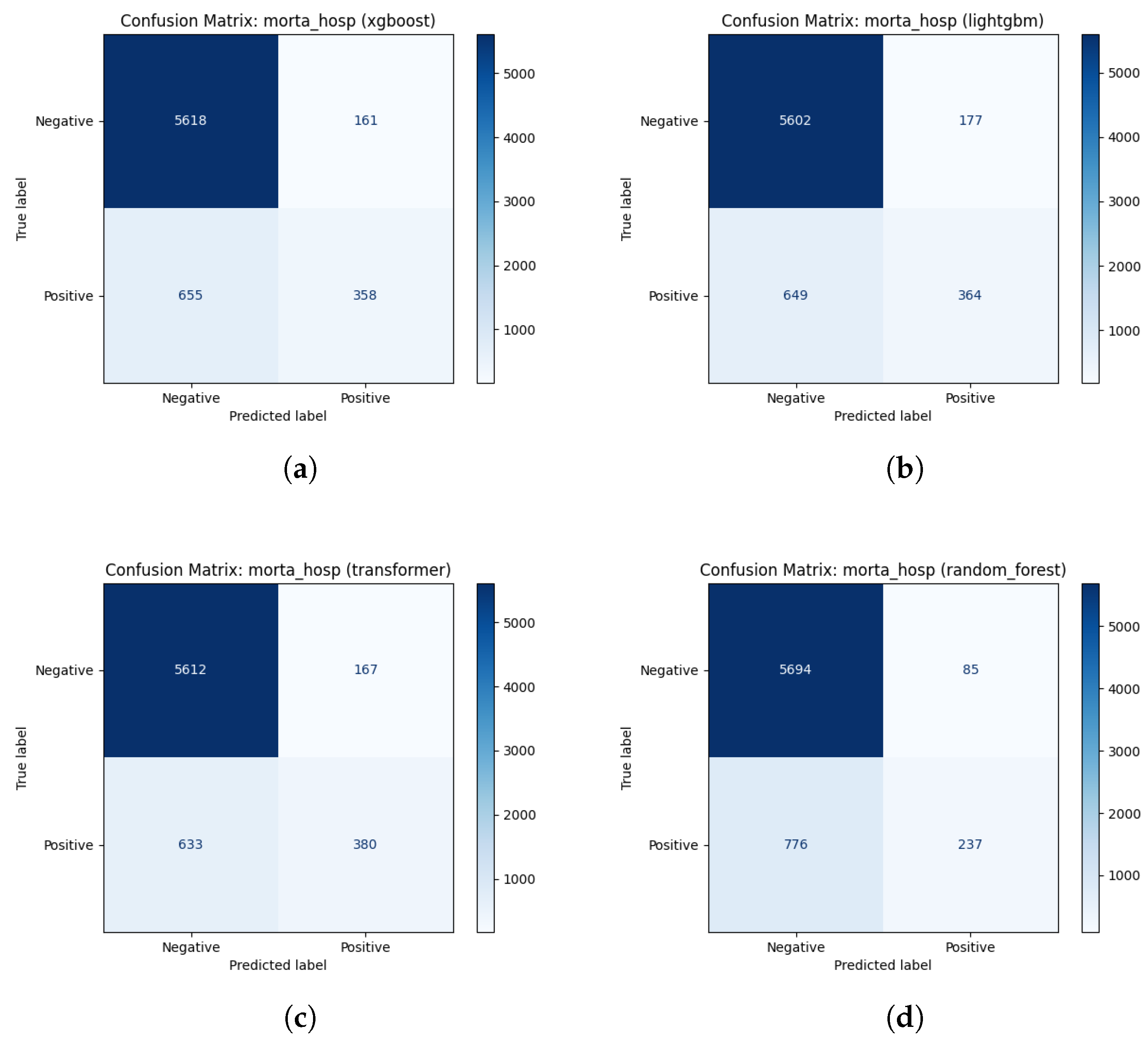
Figure 2.
Top-15 features ranked by mean absolute SHAP value for mortality prediction for XGBoost.
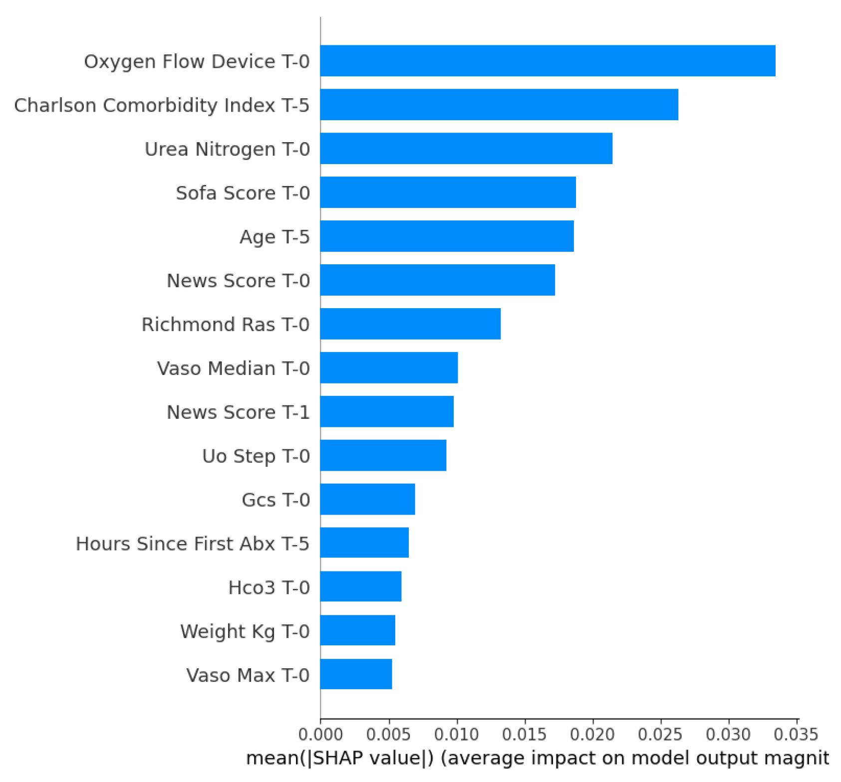
Figure 3.
SHAP beeswarm plot for Mortality used by the XGBoost model.
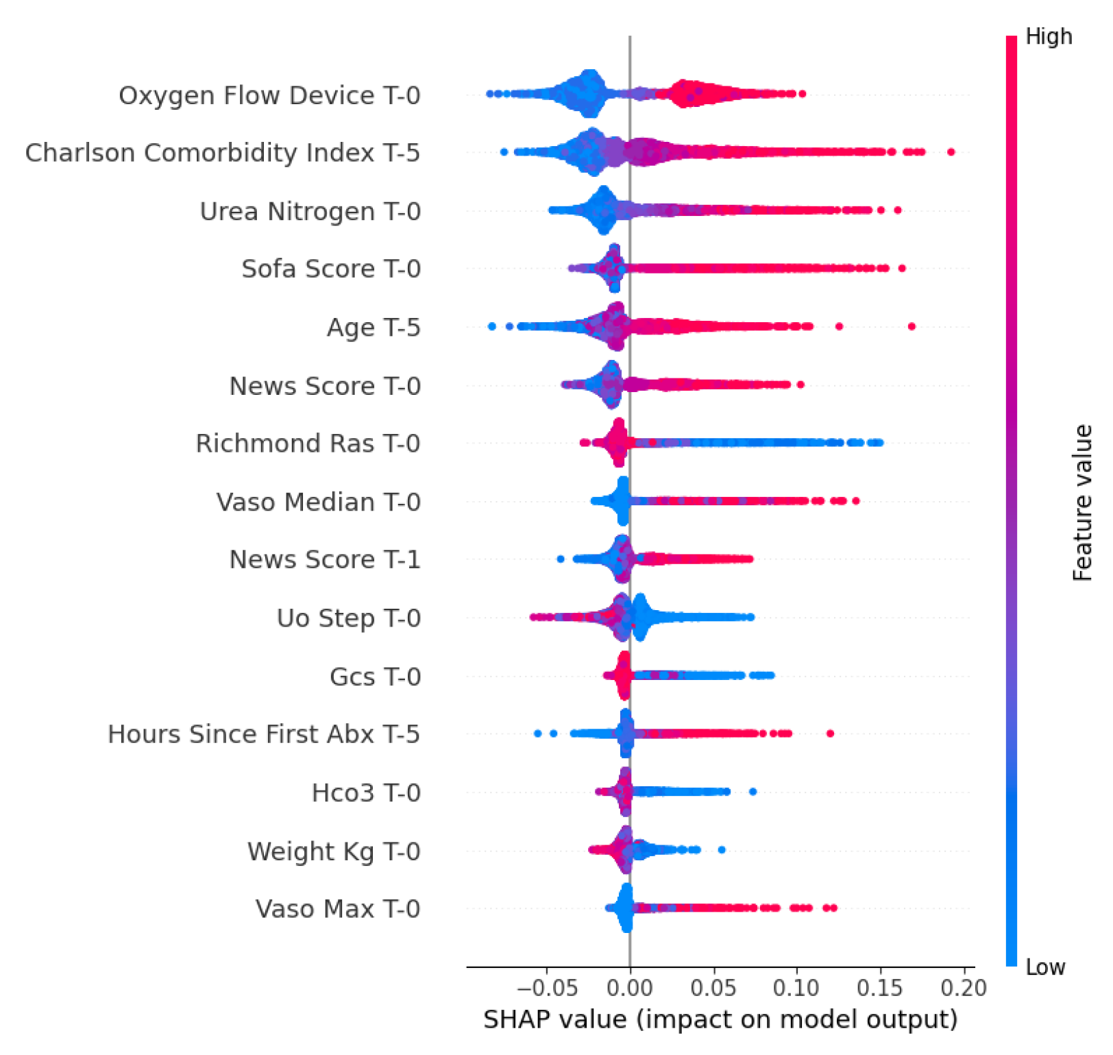
Figure 4.
SHAP waterfall plot for Mortality used by the XGBoost model.
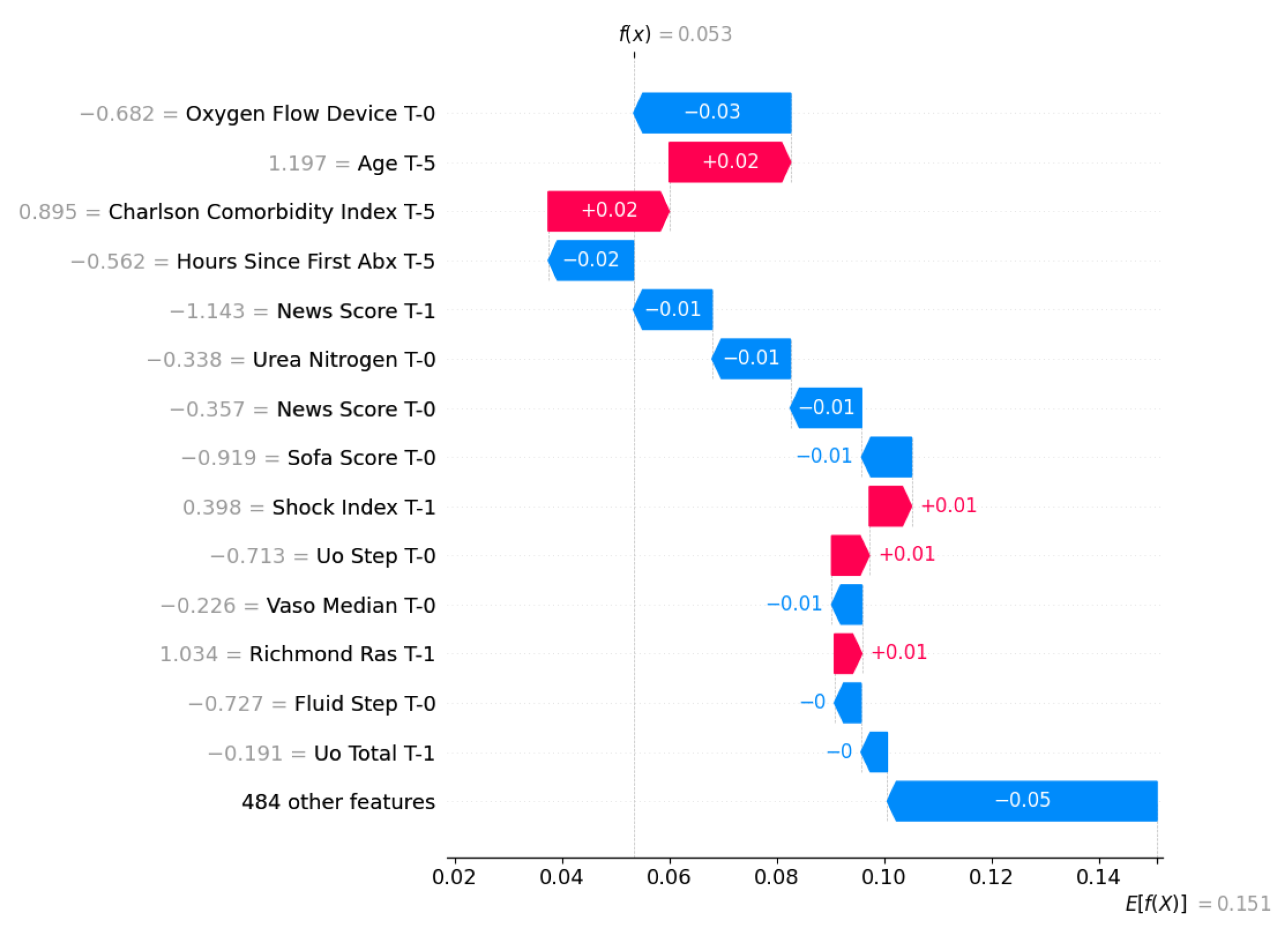
Figure 5.
Top-15 features ranked by mean absolute SHAP value for LOS task used by LightGBM.
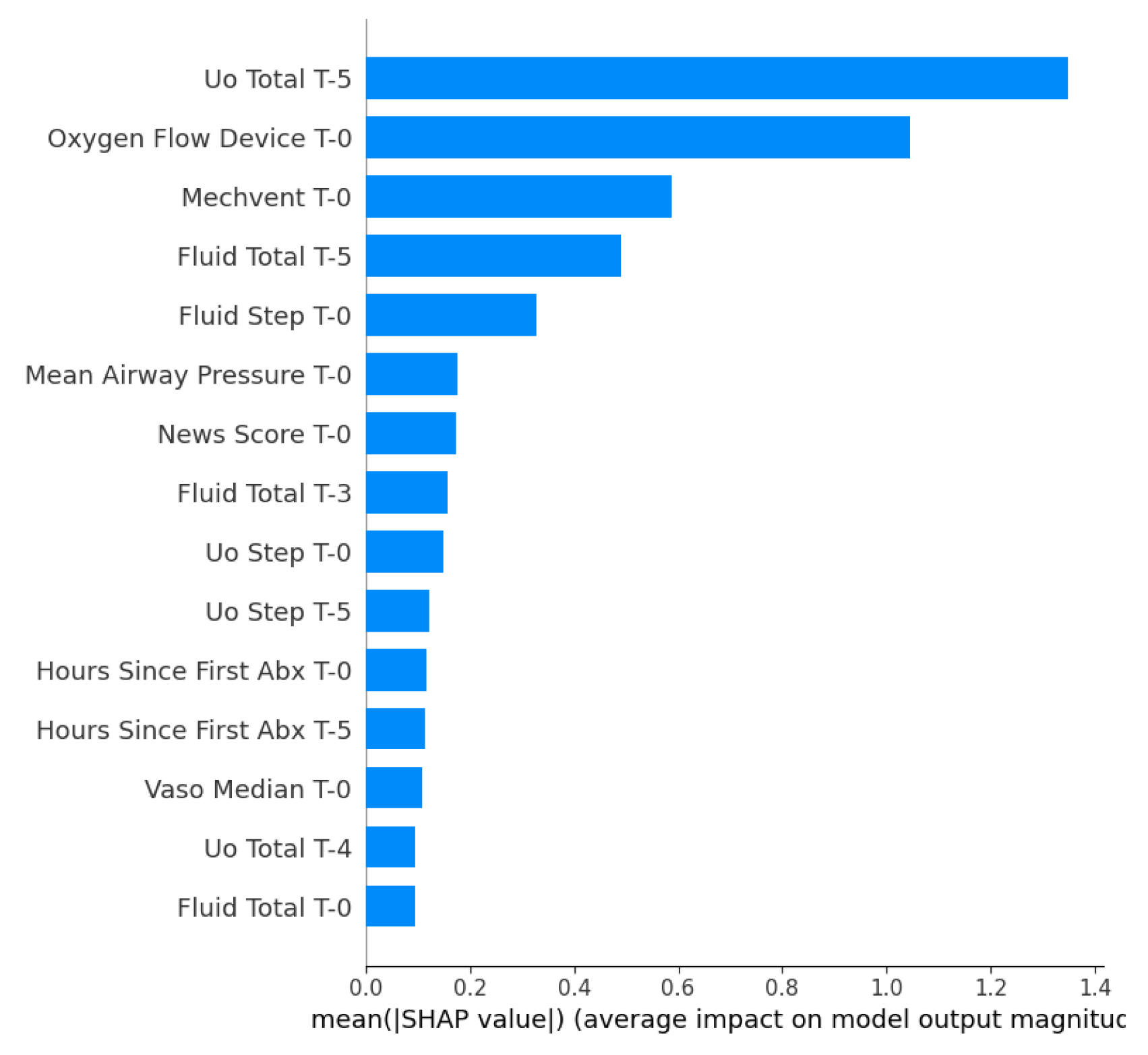
Figure 6.
SHAP beeswarm plot for LOS used by the LightGBM model.
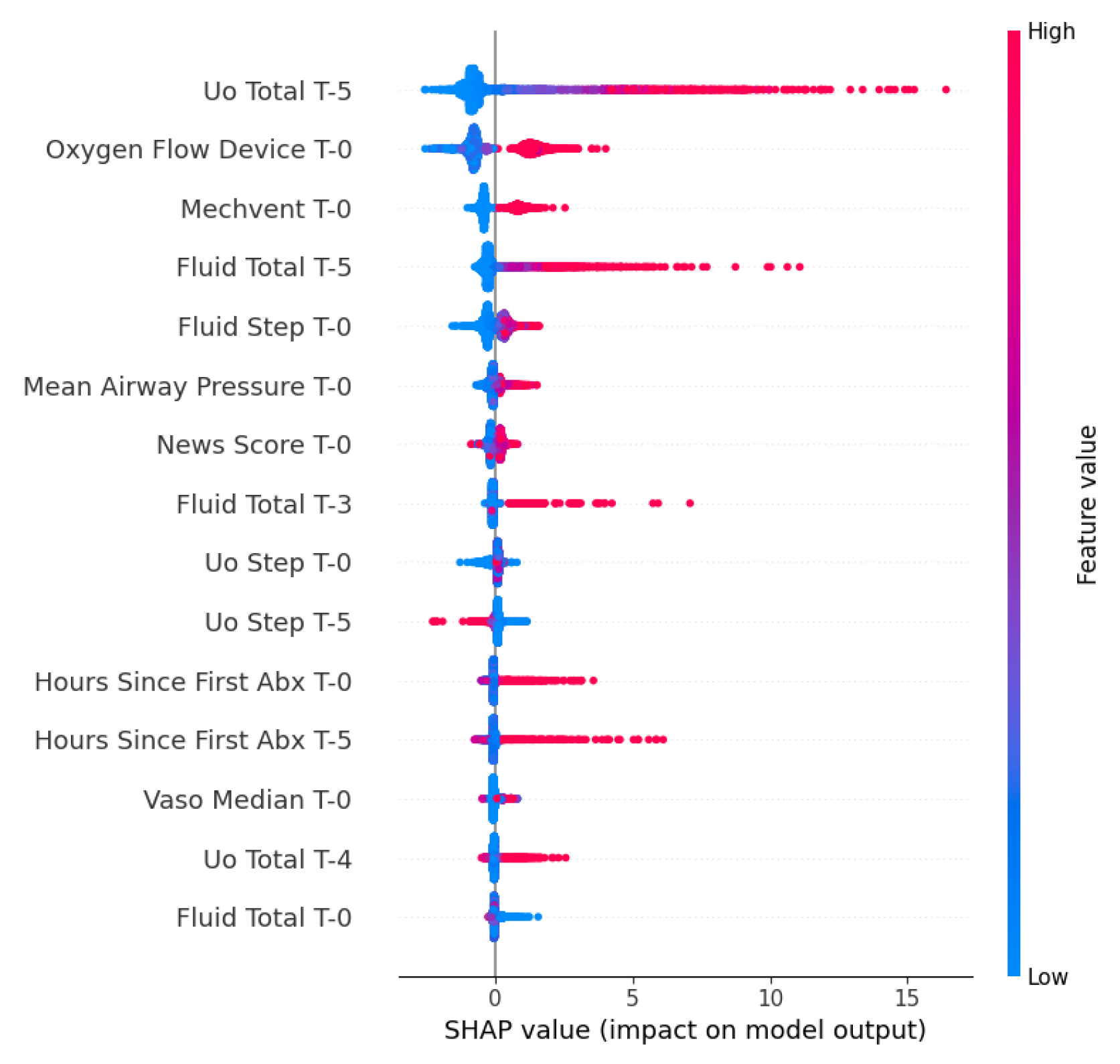
Figure 7.
SHAP Waterfall plot for LOS used by the LightGBM model.
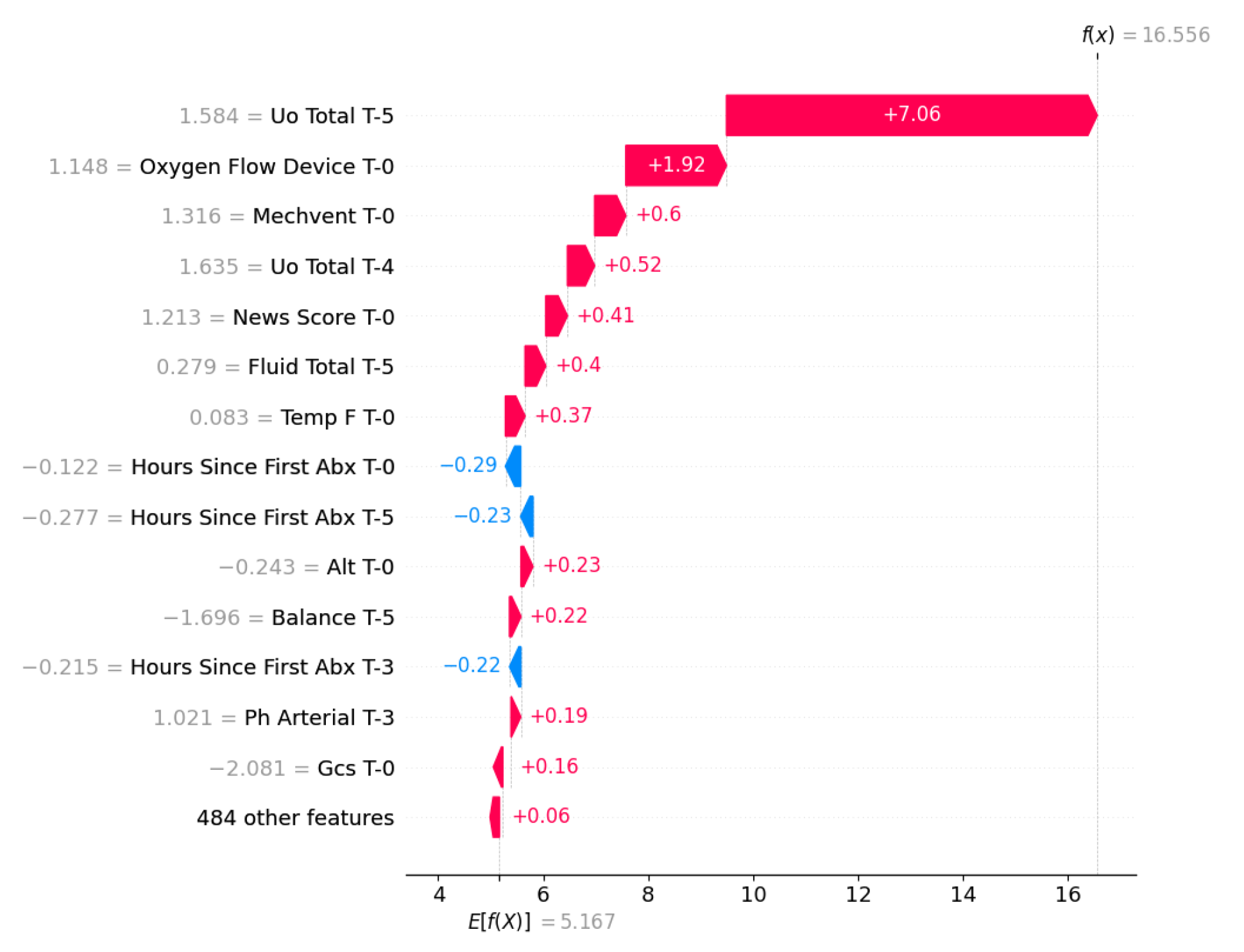
Figure 8.
Confusion Matrix for Septic Shock Task using XGBoost.
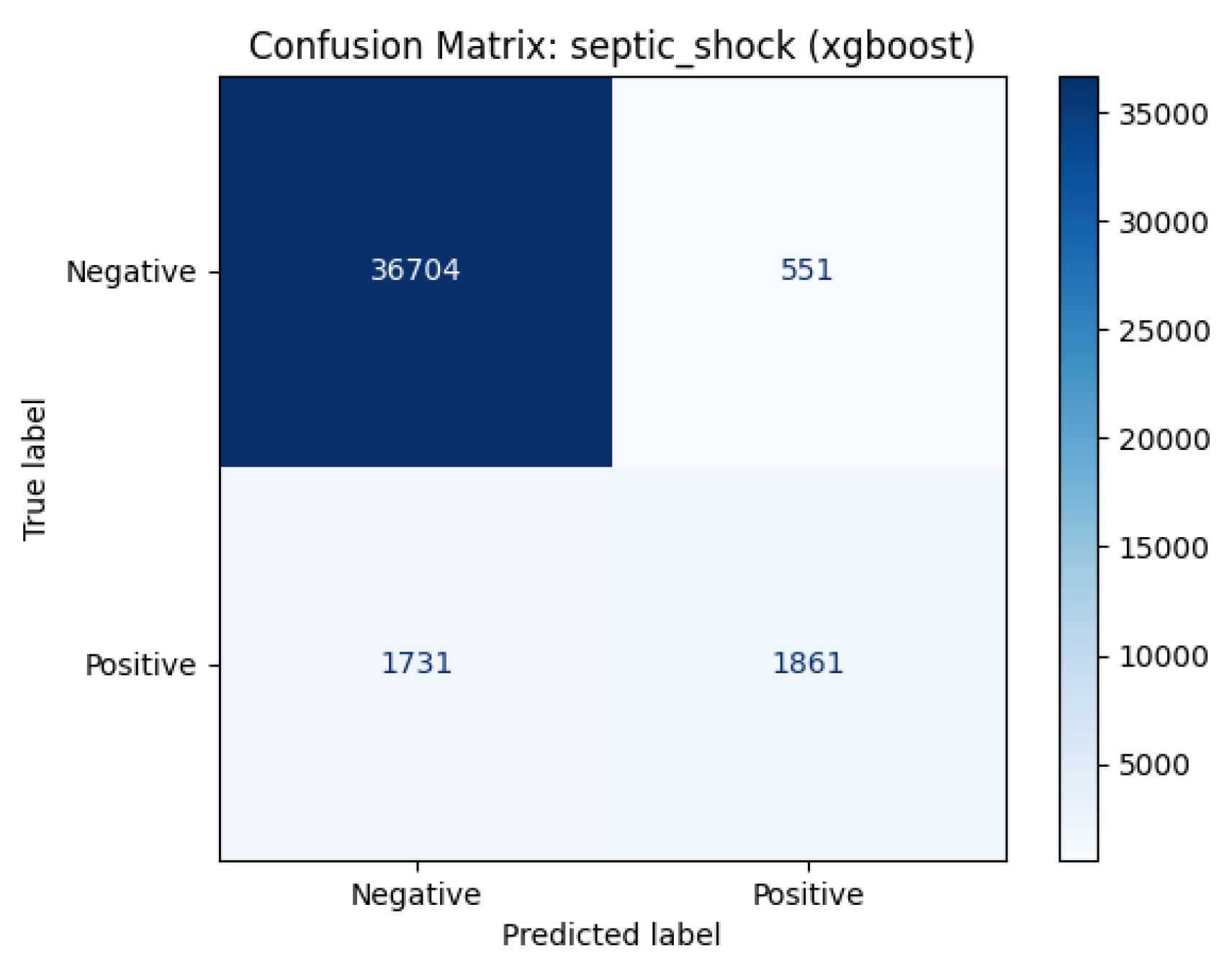
Figure 9.
Top-15 features ranked by mean absolute SHAP value for sepsis shock prediction using XGBoost.
Figure 9.
Top-15 features ranked by mean absolute SHAP value for sepsis shock prediction using XGBoost.
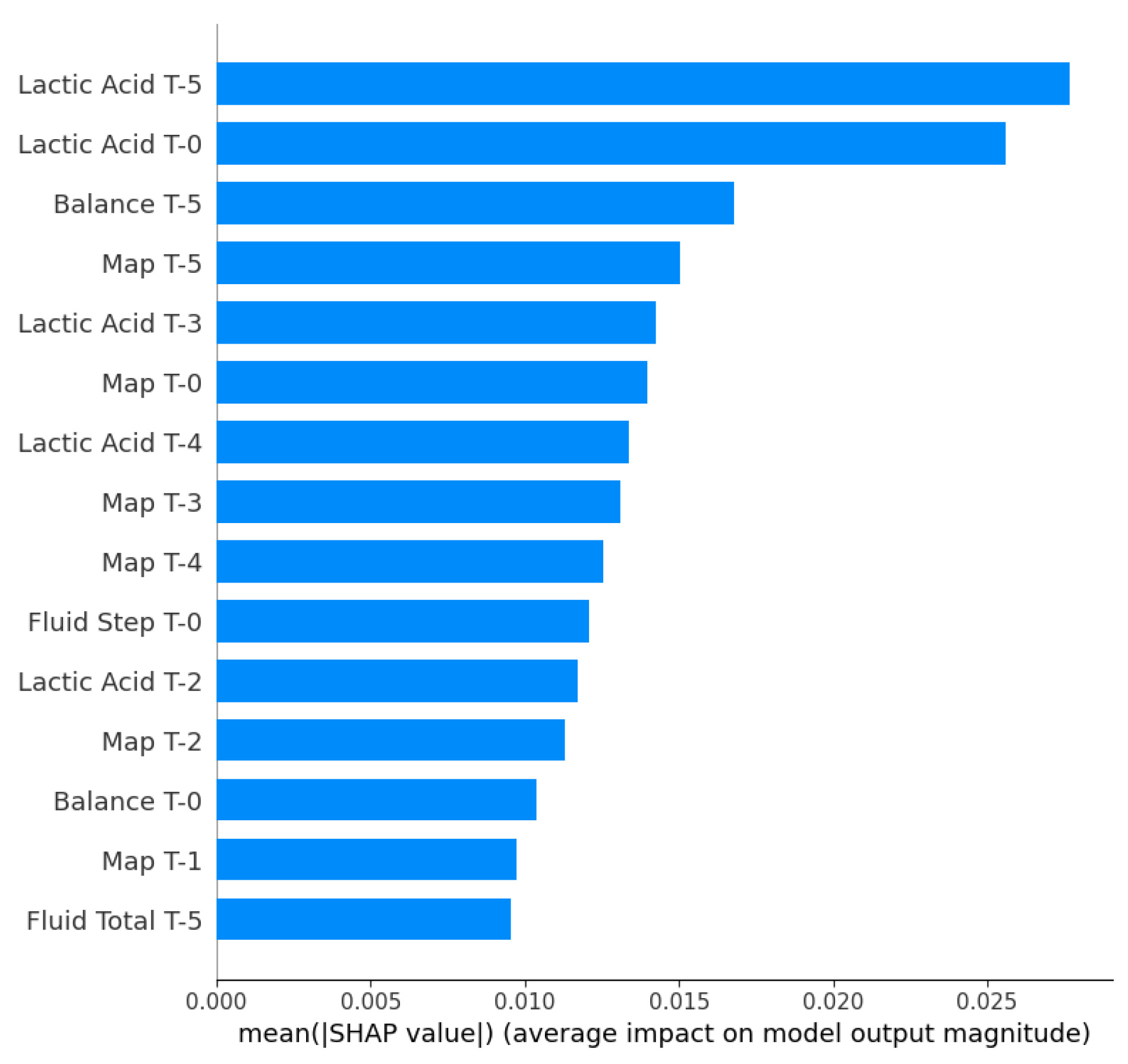
Figure 10.
SHAP beeswarm plot for septic shock prediction used by the XGBoost model.
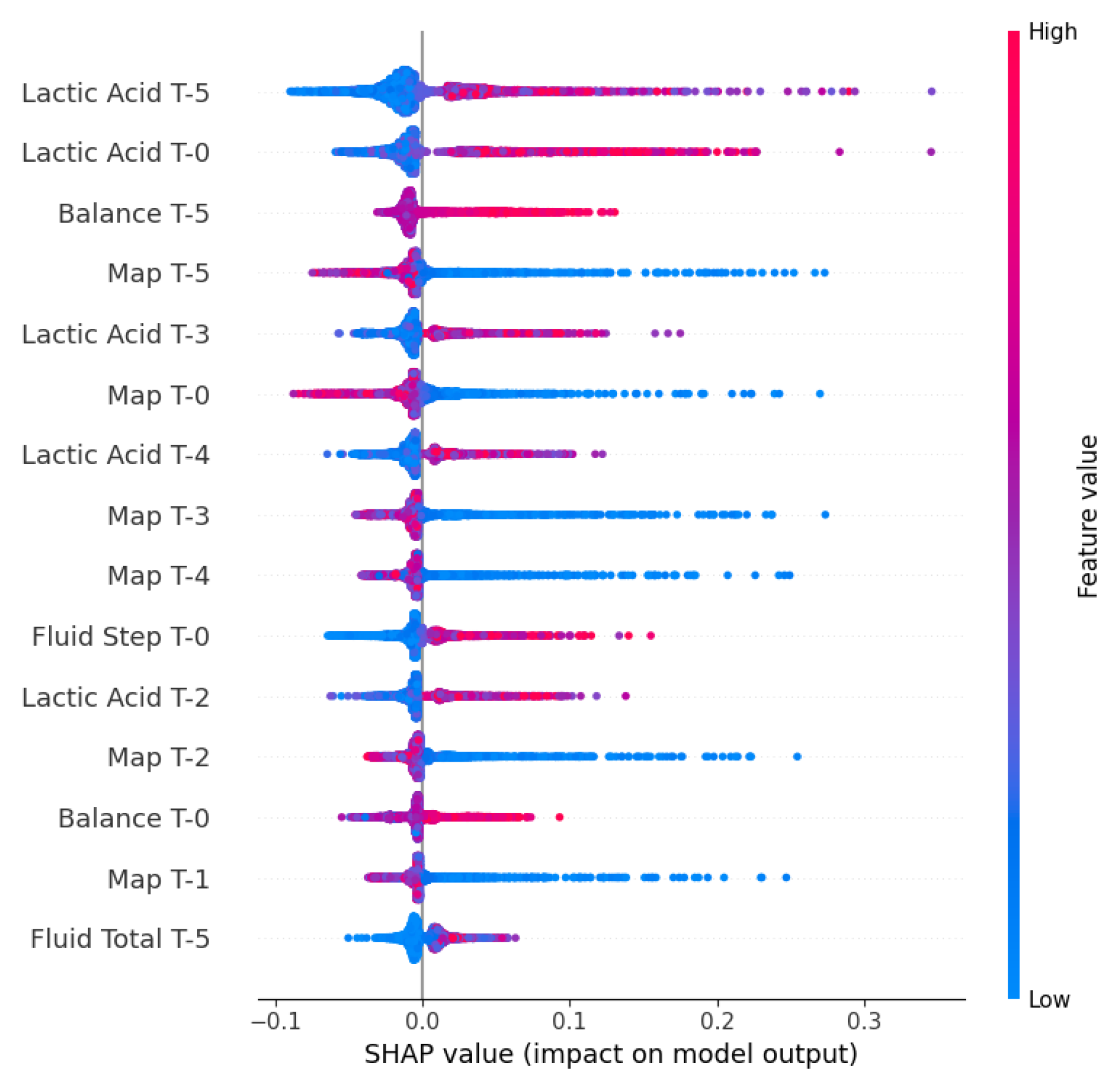
Figure 11.
SHAP waterfall plot for septic shock prediction used by the XGBoost model.
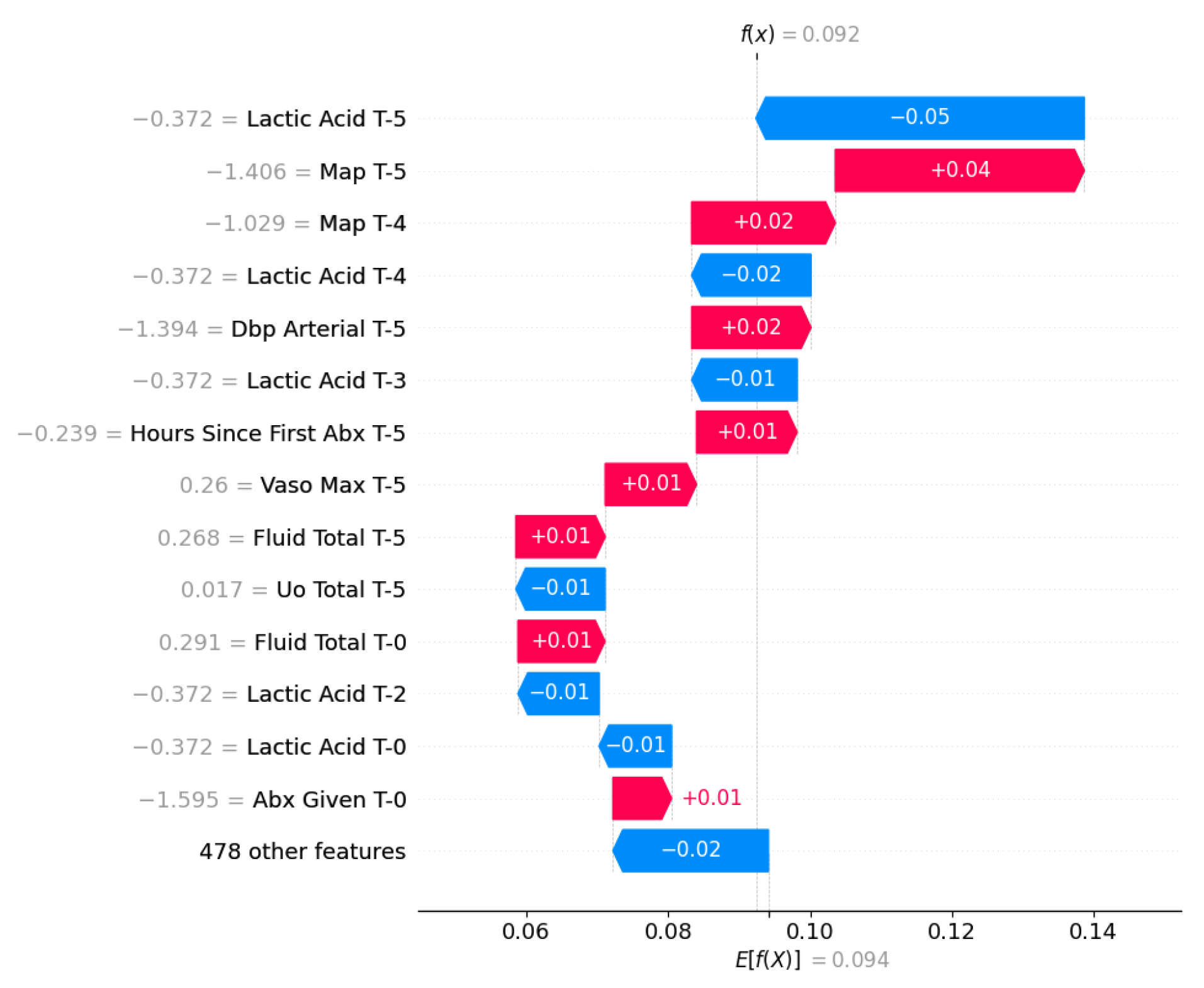
Table 1.
List of main predictor variables used in the models, grouped by clinical category.
| Category | Features |
|---|---|
| Demographics | Age, Gender, Weight, Height, Readmission Flag |
| Vital Signs | Heart Rate, Respiratory Rate, BP (Systolic, Diastolic, MAP), SpO2, Temperature, Shock Index |
| Laboratory | Glucose, Creatinine, BUN (Urea Nitrogen), Potassium, Sodium, Chloride, Magnesium, Calcium (Total, Ionized, Non-ionized), Bicarbonate (HCO3), Albumin, Lactate |
| Exams | WBC Count, Hemoglobin, Hematocrit, Platelets, RBC Count, Coagulation (INR, PT, PTT) |
| Arterial Blood Gas | pH, PaO2, PaCO2, Base Excess, Total CO2, PaO2/FiO2 Ratio |
| Ventilation | Mechanical Ventilation (Binary), FiO2, PEEP, Tidal Volume, Minute Volume, Peak Insp. Pressure, Mean Airway Pressure, Oxygen Flow/Device |
| Liver Function | ALT, AST, Bilirubin (Total, Direct) |
| Clinical Scores | SOFA Score (Total and Components), NEWS Score, SIRS Score, Glasgow Coma Scale (GCS), RASS (Sedation score), Charlson Comorbidity Index |
| Fluids, Output | Fluid Intake (Total/Step), Urine (Total/Step), Fluid Balance, Antibiotics (Given, Count, Time since 1st) |
Table 2.
Cohort Characteristics. Extended from [20].
Table 2.
Cohort Characteristics. Extended from [20].
| Category | Value |
|---|---|
| Demographics | |
| Total Patients | 35.215 |
| Age (mean ± std) | 65.4 ± 16.3 |
| Gender (% female) | 44.5% |
| Charlson Index (median [IQR]) | 5.0 [3.0-7.0] |
| Age Distribution (%) | |
| 18-40 | 8.5% |
| 41-65 | 38.1% |
| 66-80 | 33.9% |
| > 80 | 19.4% |
| BMI Distribution (%) | |
| Underweight (< 18.5) | 7.2% |
| Normal (18.5-24.9) | 29.0% |
| Overweight (25-29.9) | 26.5% |
| Obese (≥ 30) | 37.3% |
| Clinical Outcomes | |
| Hospital mortality (%) | 14.5% |
| 90-day mortality (%) | 25.1% |
| Length of stay (days) | 5.1 ± 7.1 |
| Readmission rate (%) | 7.3% |
| Septic shock (%) | 12.4% |
| Disease Severity (mean ± std) | |
| SOFA score | 5.5 ± 2.8 |
| SIRS score | 1.5 ± 1.0 |
| NEWS Score | 6.06 ± 2.57 |
| Glasgow Coma Scale | 12.87 ± 3.76 |
| Richmond Agitation-Sedation Scale | -0.94 ± 1.85 |
| Interventions | |
| Mechanical ventilation (%) | 35.1% |
| Vasopressor use (%) | 16.9% |
| Antibiotics given (%) | 66.3% |
| Patients receiving all 3 interventions (%) | 23.3% |
| Fluid Management | |
| Mean fluid balance (mL) | -931.2 ± 8142.5 |
| Fluid rate per 4h (mL) | 458.9 ± 645.2 |
| Cumulative fluid at 24h (mL) | 3017.3 ± 5566.5 |
| Patients with negative fluid balance (%) | 56.9% |
Table 3.
Statistical data for survivor and non-survivor groups.
| Variable | Survivors | Non-Survivors | P-Value |
|---|---|---|---|
| (n=30105) | (n=5110) | ||
| Demographics | |||
| Age, median [IQR] | 66.0 [55.0-77.0] | 71.0 [60.0-81.0] | |
| Male Sex, n (%) | 13463 (44.7%) | 2222 (43.5%) | 0.103 |
| Charlson Index, median [IQR] | 5.0 [3.0-7.0] | 6.0 [4.0-9.0] | |
| Clinical Scores (Admission) | |||
| SOFA Score, median [IQR] | 5.0 [3.0-7.0] | 7.0 [5.0-9.0] | |
| NEWS Score, median [IQR] | 6.0 [4.0-7.0] | 7.0 [6.0-9.0] | |
| SIRS Score, median [IQR] | 2.0 [1.0-2.0] | 2.0 [1.0-3.0] | 1.000 |
| Vital Signs (Admission) | |||
| Heart Rate (bpm), median [IQR] | 87.0 [75.7-100.8] | 91.5 [78.7-106.2] | |
| MAP (mmHg), median [IQR] | 79.2 [70.6-89.6] | 75.6 [67.6-85.8] | |
| Respiratory Rate (bpm), [IQR] | 19.3 [16.3-23.0] | 21.4 [18.0-25.2] | |
| SpO2 (%), median [IQR] | 97.2 [95.2-99.0] | 96.9 [94.7-98.8] | |
| Temperature (C), median [IQR] | 36.8 [36.5-37.2] | 36.8 [36.4-37.2] | 1.000 |
| Laboratory Values (Admission) | |||
| Lactate (mmol/L), median [IQR] | 1.6 [1.1-2.4] | 2.0 [1.3-3.3] | |
| Creatinine(mg/dL), median [IQR] | 1.0 [0.7-1.5] | 1.3 [0.8-2.2] | |
| Bilirubin (mg/dL), median [IQR] | 0.6 [0.4-1.4] | 0.8 [0.4-2.2] | |
| Platelets (K/uL), median [IQR] | 197.0 [137.0-271.0] | 174.0 [103.0-259.0] | |
| WBC (K/uL), median [IQR] | 10.4 [7.2-14.6] | 12.4 [8.3-17.8] | |
| Outcomes | |||
| LOS (hours), median [IQR] | 2.3 [1.3-5.0] | 4.9 [2.5-9.7] | |
Table 4.
Tasks descritptions.
| Task | Type | Approach | Metrics |
|---|---|---|---|
| Mortality | Binary Classification | Static (initial 24h) | AUROC, AUPRC, Accuracy |
| LOS | Regression | Static (initial 24h) | RMSE, MAE |
| Septic Shock | Binary Classification | Dynamic (last 24h) | AUROC, AUPRC, Accuracy |
Table 5.
Results for Mortality Prediction.
| Model | AUROC | AUPRC | Accuracy |
|---|---|---|---|
| XGBoost | 0.874 | 0.606 | 0.881 |
| LightGBM | 0.874 | 0.597 | 0.879 |
| Transformer | 0.854 | 0.565 | 0.876 |
| Random Forest | 0.854 | 0.556 | 0.875 |
| Logistic Regression | 0.845 | 0.527 | 0.870 |
| LSTM | 0.824 | 0.507 | 0.856 |
Table 6.
Results for Length of Stay Prediction.
| Model | RMSE | MAE | MSE |
|---|---|---|---|
| LightGBM | 4.801 | 2.599 | 23.045 |
| XGBoost | 4.912 | 2.601 | 24.128 |
| Random Forest | 4.950 | 2.740 | 24.507 |
| LSTM | 5.049 | 2.726 | 25.493 |
| Transformer | 5.486 | 2.811 | 30.093 |
| Linear Regression | 5.499 | 2.885 | 30.242 |
Table 7.
Results for Septic Shock Prediction.
| Model | AUROC | AUPRC | Accuracy |
|---|---|---|---|
| XGBoost | 0.955 | 0.799 | 0.956 |
| LightGBM | 0.954 | 0.790 | 0.953 |
| Transformer | 0.947 | 0.742 | 0.946 |
| Random Forest | 0.934 | 0.732 | 0.948 |
| LSTM | 0.898 | 0.583 | 0.923 |
| Linear | 0.880 | 0.455 | 0.919 |
Disclaimer/Publisher’s Note: The statements, opinions and data contained in all publications are solely those of the individual author(s) and contributor(s) and not of MDPI and/or the editor(s). MDPI and/or the editor(s) disclaim responsibility for any injury to people or property resulting from any ideas, methods, instructions or products referred to in the content. |
© 2026 by the authors. Licensee MDPI, Basel, Switzerland. This article is an open access article distributed under the terms and conditions of the Creative Commons Attribution (CC BY) license (http://creativecommons.org/licenses/by/4.0/).
Copyright: This open access article is published under a Creative Commons CC BY 4.0 license, which permit the free download, distribution, and reuse, provided that the author and preprint are cited in any reuse.


