Submitted:
06 February 2026
Posted:
09 February 2026
You are already at the latest version
Abstract
The constant external electric field, applied to a semiconductor nanostructure, changes the symmetry. It can be cylindrical symmetry, for the field parallel to the z-axis, or a symmetry breaking, for the field parallel to the x-y plane. The symmetry changes affect the optical properties of the system, which are subject of the presented considerations. Below we present a theoretical calculation of optical functions for CdSe Nanoplatelets with excitons, in an external homogeneous electric field. We consider various configurations, with the external field perpendicular and parallel to the platelet planes. With the help of the real density matrix approach, we calculate the linear electro-optical functions of CdSe nanoplatelets, taking into account the effect of a dielectric confinement on excitonic states. The impact of platelet geometry (thickness, lateral dimension), and on the applied field strength, on the spectrum, is discussed.
Keywords:
electroabsorption
; nanoplatelets
; CdSe
; exciton states
; Franz-Keldysh effect
1. Introduction
We concentrate our attention on semiconductor nanostructures, called nanoplatelets (NPL), which are quantum dots (QDs), but with different confinement mechanism, compared with other (for example GaAl/GaAlAs) QDs and quantum wells (QWs) which we call standard QDs (QWs). In the standard QDs the electrons and the holes, created by the wave propagating in a QW, are confined in a nanostrukture of one type of semiconductors by an impenetrable barrier of a different semiconductor. In the considered below CdSe NPLs the confinement is of electrostatic origin and is made by a large dielectric contrast between the semiconductor (here CdSe) and its environment. Despite this difference, electrons and holes interact by a screened Coulomb potential, and bound electron-hole pairs, named excitons, are created. Colloidal group II-VI semiconductor nanostructures have emerged as one of the most studied inorganic systems. The quite uncomplicated synthesis and the ability to tune optical properties depending on their crystalline size due to the quantum confinement effect1 make them good candidates for highly efficient light emitters, bioimaging markers, and photovoltaic cells. Colloidal nanoplatelets (NPLs) are cuboid nanostructures with the thickness of several atomic layers and much larger lateral size so that the confinement is strong only in the thinnest dimension. In the two last decades, after the first synthesize of CdSe NPLs, [1], a large number of works dedicated to this topic, appeared. A small selection of them is given in references [1]-[18].
As in standard QDs, the optical properties of NPLs are dominated by excitons. So the major part of the initial research on NPLs was concentrated on the calculation of exciton characteristics, such as exciton binding energy, confinement eigenfunctions, and eigenvalues.
Similar to the case of other nanostructures, the next development was directed at electro- and magneto-optical properties. CdSe nanoplatelets (NPLs) have unique electro-optical properties due to strong 1D quantum confinement, featuring giant oscillator strength (GOST), narrow absorption/emission, large absorption cross-sections, high exciton binding energies, and excellent optical gain, making them ideal for LEDs, lasers, and sensors, with thickness dictating color and surface chemistry (ligands/doping) tuning efficiency and spectral features like their strong Stark effect under electric fields. Beginning with the pioneering work by Miller et. al. [19], where the term ’Quantum Confined Stark Effect’ (QCSE) was introduced, the optical response of quantum semiconductor nanostructures (wells, dots, wires) subjected to an interaction with the external constant electric field, has attracted many interest over the past decades, for example, [20]-[22]). Besides the cognitive value, this attention is motivated by possible technological applications of QCSE, for example, Self-Electrooptic Effect Devices (SEEDs), fast optical switches and modulators, crucial for optical communications (for example, [23]).
The optical properties of NPLs, including electro-absorption, were subject of extensive experimental and theoretical studies (for example, [22]). However, it seems, that there are few theoretical articles on electro-optical effects. This makes an inspiration to the present work. We will discuss the effects of applied static electric field on NPL with dielectric confinement. The electron-hole Coulomb potential dielectrically screened with the static dielectric constant is adopted, and the valence band structure is considered in the cylindrical approximation, thus separating light- and heavy hole motions. In calculations we use the so-called Real Density Matrix Approach (RDMA) (see Ref. [24] for details about RDMA). This method enables to obtain analytic expressions for the NPLs electro-optical functions, where we have chosen the electro-absorption coefficient.
The paper is organized as follows. In Sect. 2 we present the calculation method, based on RDMA. In Section 3 and Section 4 we discuss the case of the electric field applied parallel to the NPL growth axis (z-axis). In the next section we analyze the case of the field applied parallel to the NPL plane, when the exciting electromagnetic wave energy is below the fundamental gap. The case with the field applied parallel to the NPL plane, when the exciting wave energy exceeds the fundamental gap, is discussed in Sect. 6. We close with conclusions in Sect. 7. Appendices A and B contain calculation details.
2. The Method
The real density matrix approach (RDMA) seems to be especially appropriate for computing the effects of external fields since it includes both the relative motion of the carriers and the center-of-mass motion, where the interaction with the radiation field takes place.
We analyze the weak field limit, where the set of basic RDMA equations (’constitutive equations’) reduces to a set of linearized equations which are the inter-band equations with only the linear source on the right-hand-side retained. The resulting linearized equations for the coherent amplitudes for the electron-hole pair of coordinates and between any pair of bands (valence band) and b (conduction band) read:
where is a phenomenological damping coefficient, E is the electric vector of the impinging electromagnetic wave, and is the inter-band transition dipole density. The notation is used. When external static fields F (electric field), and B (magnetic field), are applied, the effective-mass two-band Hamiltonian with gap for any pair of bands is
choosing appropriate values of and the effective mass tensors , and are the surface potentials for electrons and holes. The coherent amplitudes determine the total NPL polarization
where the summation includes all allowed excitonic transitions between the valence and conduction bands, R and r are the electron-hole pair center-of-mass and the relative coordinate, respectively. The equations (1)-(3) connect the polarization to the electric field. In addition, the electric field must obey the Maxwell equation
where the polarization is given in Eq.(3), and is the dielectric constant of the material contained inside the NPL.
- 1.
- 2.
- Having calculated the amplitudes, we use them in Eq. (3) and, in the long wave approximation, determine the NPL susceptiblity.
- 3.
- The so obtained susceptibility enables to calculate the optical functions (electro-reflectivity, transmissivity, absorption).
We consider dipole-allowed transitions at the point of the Brillouin zone within a simple two-band model. Further, we assume that the electric field E is linearly polarized with a component and that the vector M has a non-vanishing component in the same direction. For the quantities the center-of-mass dependence is of the plane-wave form . As in previous works, in the NPL internal region we separate the exciton center-of-mass and relative motion, and consider the case . This assumption forces the cylindrical symmetry, and the Hamiltonian (2) is transformed into the form
where the cyclotron frequency is
and the reduced mass is defined as
The operator is the z-component of the angular-momentum operator. We must solve the constitutive equations with the above Hamiltonian to obtain the polarization and finally the optical functions. Since we aim to analyze the electro-optical effects, all terms in the Hamiltonian (5) related to the magnetic field will be put equal zero.
3. The Electric Field Parallel to the Z-Axis
We will discuss the changes of the NPL optical response when a constant external electric field F is applied in the z-direction. We consider a CdSe nanoplatelet of cuboid shape, located at the plane, and with the barriers located at . Typically, for NPLs the vertical dimension (’thickness’) is of the order of a few monolayers, which, for example, in the below considered CdSe NPLs, means 1-2 nm. The lateral extension is much larger, mostly several dozen nm. A schematic picture of a nanoplatelet is displayed in Figure 1.
As was merely proved, the small vertical extension forces changes in electron and hole effective masses. They increase with decreasing thickness. This situation is illustrated in Table 1. We consider the response of the NPL to a normally incident electromagnetic wave, linearly polarized in the x-direction

Table 1.
Masses, reduced masses, Rydberg energies, Luttinger parameters, and coherence radii, from Ref. [14]. Lengths in nm, masses in free electron mass , energies in meV, ML means ’monolayers’.
Table 1.
Masses, reduced masses, Rydberg energies, Luttinger parameters, and coherence radii, from Ref. [14]. Lengths in nm, masses in free electron mass , energies in meV, ML means ’monolayers’.
| Parameter | 3ML | 4ML | 5ML |
| 1 | 1.33 | 1.67 | |
| 0.2567 | 0.2015 | 0.1635 | |
| 0.3208 | 0.2519 | 0.2044 | |
| 1.236 | 1.575 | 1.94 | |
| 1.1925 | 0.9754 | 0.8153 | |
| 0.4957 | 0.4337 | 0.3879 | |
| 0.4149 | 0.3659 | 0.3302 | |
| 0.8121 | 0.6887 | 0.5963 | |
| 0.2112 | 0.167 | 0.1362 | |
| 0.1586 | 0.13 | 0.1094 | |
| 1.236 | 1.575 | 1.94 | |
| 0.989 | 1.26 | 1.55 | |
| 0.266 | 0.325 | 0.389 | |
| 0.765 | 0.867 | 0.961 | |
| 918.13 | 686.81 | 530 | |
| 221.13 | 162.1 | 130 | |
| 579.53 | 352.26 | 277.58 | |
| 1139.4 | 816.8 | 636 | |
| 1497.4 | 1036.5 | 783.1 | |
| 96.98 | 76.12 | 61.77 | |
| 73.58 | 60.20 | 51.28 | |
| 450.5 | 368.5 | 308 | |
| 156.74 | 138.23 | 124,66 | |
| 86.88 | 69.67 | 57.49 | |
| 1.6243 | 1.8789 | 2.1062 | |
| 0.3929 | 0.4269 | 0.4488 | |
| 0.20 | 0.18 | 0.17 | |
| 0.22 | 0.19 | 0.18 |
The movement of electrons and the holes in the z direction is affected by the dielectric confinement potential, which we take in the form
The coefficient is proportional to dielectric permittivities [25]-[27]
where and are the permittivities of surrounding environment (ligands) and internal media, respectively, and . Using the potential (9) we solve the corresponding Schrödinger equation [14]. The resulting eigenvalues, demonstrating the impact of the permittivities, are given in Appendix A, Eq. (A1). In the calculations we have used the values [5].
The calculations of electro-optical properties become much simpler when we consider an NPL of thickness , with parabolic confinement potentials in the form of an harmonic oscillator potential
where the energies correspond to the electron and hole barriers. When concerning the in-plane electron and hole motion, we retain the assumptions presented in Ref. [14], where the cuboidal NPL is replaced by a cylinder of hight , and a radius We neglect the motion of the hole, and the electron moves under the influence of the Coulomb attraction with the hole located at the point , and the confinement potential
where we put . In this case, and with the applied constant electric field, the NPL Hamiltonian has the form
containing the one-dimensional oscillator Hamiltonians
and the two-dimensional Coulomb Hamiltonian
Using the substitution
we obtain the QW Hamiltonians in the form
With the above QW Hamiltonians we can solve the constitutive equations
We use the long wave approximation, and seek solutions in the form
where are the eigenfunctions of the Hamiltonian (15),
Here j and m are the principal and magnetic quantum numbers of the 2-dimensional excitonic state, is the confluent hypergeometric function (notation by Ref. [28]), , and we used notation
where is the free electron mass, and the hydrogen Bohr radius. The functions (N=0,1,...) are the quantum oscillator eigenfunctions of the Hamiltonian (14),
being Hermite polynomials . We consider in detail the lowest confinement state .
For further calculations we must define the dipole density M. Having in mind the experiments from Refs. [22], and [6], where resonances due to 1SH and 1SL excitons were observed, we choose M in the form
where are the so-called coherence radii
and are normalization constants
The integrated dipole strengths for CdSe NPLs od various sizes, are given in Ref. [14]
Inserting the series (20) into constitutive equation (19) we calculate the expansion coefficients . The so obtained exciton amplitudes are used in Eq. (3), giving the NPL polarization and, by relation , the susceptibility
where the summation runs over the excitonic transitions taken into account. The exciton resonance energies are defined by the relation
where
and are the eigenvalues of the operator (15), is the Stark shift. The excitonic binding energy is defined as
4. Results of Specific Calculations for
We performed calculations for 3 CdSe nanoplatelets analyzed in Ref. [6], with sizes
- 3ML ,,
- 4ML ,
- 5 ML .
All the parameters used in the calculations are collected in Table 1. We have calculated the Stark shift, depending on the lateral dimension , and the applied field strength F, obtaining the result
where
and is the total exciton mass in the z-direction. The quantity represents the ionization field strength
The details of the calculations are given in Appendix A
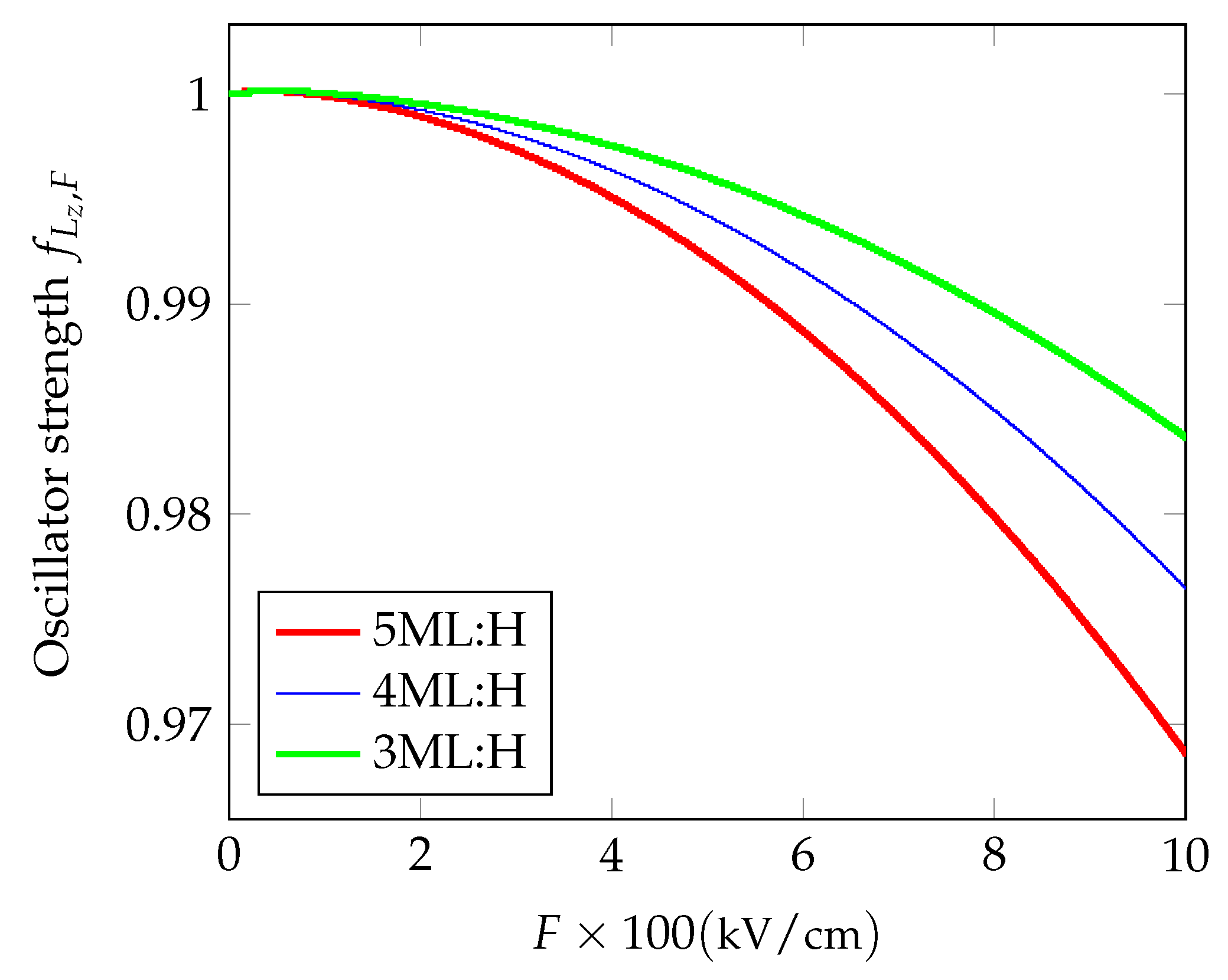
Using the eigenfunctions (22), and the dipole densities (23), we calculated the oscillator strengths (the part related to the vertical motion), obtaining the expression
The dependence on the applied field strength is depicted in Figure 2. We observe the decreasing of oscillator strengths with the increasing field strength.
Figure 3.
Oscillator strengths dependence on applied field strength.
Finally, we have calculated the absorption coefficient, as the imaginary part of the susceptibility (26). In this equation the resonance energies are needed. An important component of the resonance energy is the exciton binding energy, defined in Eq. (31). We observe that the binding energy decreases with the increasing field, as shown in Figure 4 In consequence, the resonance energies increase, despite of the Stark shift, acting in opposite direction. The absorption maxima are shifted versus higher energies (smaller wave lengths), in difference to the behavior in quantum wells. Such shift was observed in experiments by Baghdasaryan et al. [22]. Besides, the heavy- end light exciton absorption maxima are nearing and merge in the limit of high fields (Figure 6). The dependence of the binding and resonance energies, and the absorption coefficient, on the applied field strength, is shown in Figure 4, Figure 5 and Figure 6.
Figure 4.
Exciton binding energy for heavy holes versus applied field strength.
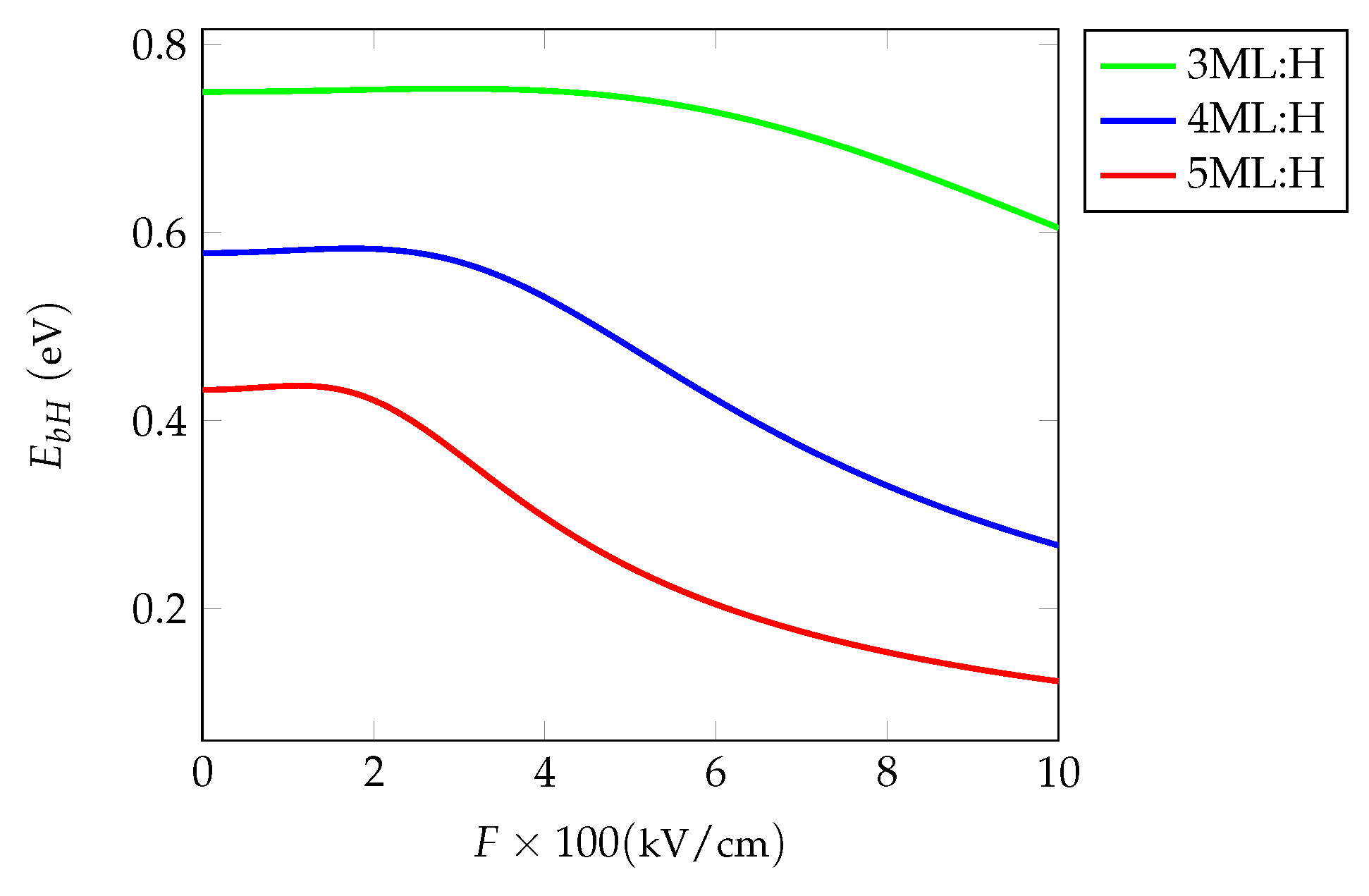
Figure 5.
Resonance energies for heavy (H) and light (L) hole exciton vs applied field strength.
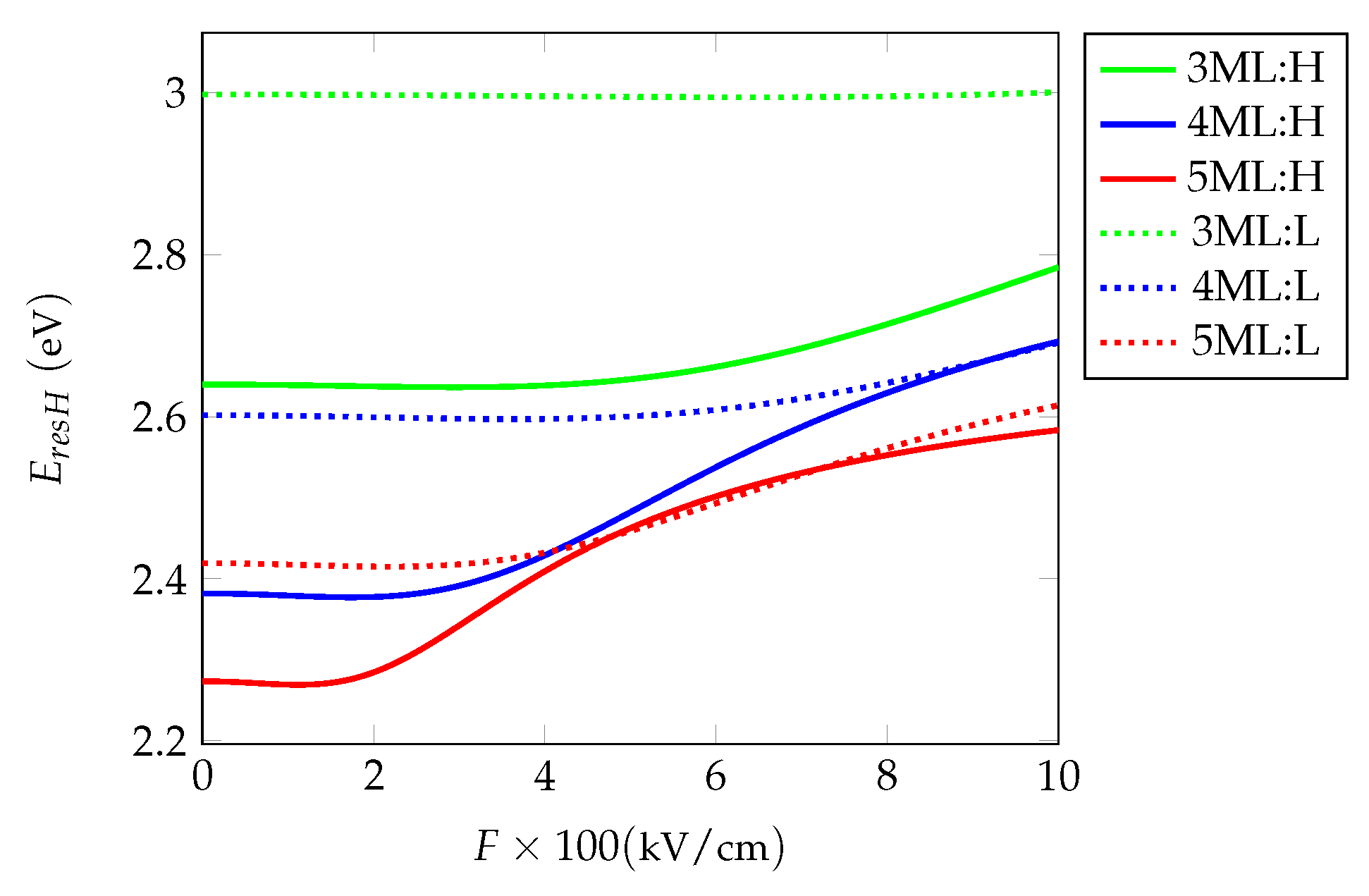
Figure 6.
Normalized absorption for the case ’Thickness’ at 273 K, for three values of the applied field in the case 4ML thickness. The dashed curve represents experimental data from Ref. Geiregat et al. [9]
Figure 6.
Normalized absorption for the case ’Thickness’ at 273 K, for three values of the applied field in the case 4ML thickness. The dashed curve represents experimental data from Ref. Geiregat et al. [9]
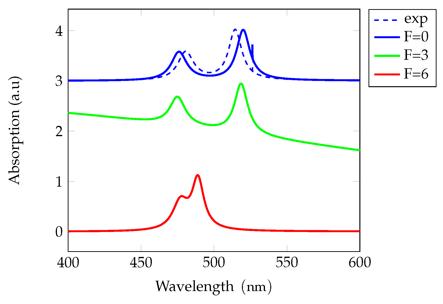
Table 2.
Sizes and exciton states energies, transition matrix elements M, oscillator strengths, and damping parameters, for disks analyzed by Brumberg et al. [6], lengths in nm, matrix elements M in , energies in meV, the energy gap at room temperature 1750 meV, notation: 1: , 2: 3: , 4: , 5: , 6: .
| lat. extension | 1 | 2 | 3 | 4 | 5 | 6 |
| 1 | 1.26 | 1.553 | 1.26 | 1.26 | 1.26 | |
| 27 | 9 | 10.25 | 9 | 10.25 | 27 | |
| 27 | 7.15 | 6.6 | 7.15 | 8.134 | 21.455 | |
| 1SH | 2640.44 | 2382.2 | 2242.2 | 2540 | 2537.7 | 2531 |
| 469.2 | 520.5 | 553 | 488.6 | 489 | 490.4 | |
| 1SL | 3178.4 | 2745.25 | 2498.4 | 2761 | 2758.7 | 2752 |
| 390 | 451.68 | 496.31 | 449.5 | 449.8 | 450.9 | |
| 0.625 | 0.22 | 0.19 | 0.22 | 0.19 | 0.625 | |
| 4.16 | 4.77 | 5.47 | 4.77 | 4.6 | 4.96 | |
| 3.72 | 3.75 | 4.77 | 3.75 | 4.44 | 4.41 | |
| 4.63 | 2.53 | 2.86 | 2.53 | 2.86 | 2.86 |
5. The Electric Field Parallel to the NPL Plane, Excitation Below Gap
In this section we analyze the electro-optical effects, when the external electric field F is applied parallel to the NPL-plane, choosing the axis . The considered case is more complicated than the case , where the electric field was decoupled from the 2-dimensional Coulomb potential, acting in the plane. Here the field, parallel to the x-axis, acts in the same plane as the cylindrically symmetric Coulomb potential, which makes impossible to find analytic solution of the relevant Schrödinger equation. To have an insight into the effects of the electric field, we have chosen a 2-dimensional model, where the electron is moving along the x axis in the interval , and we maintain the electron and hole movement in the z-direction, in the plane . With this assumptions the relevant Hamiltonian has the form
where
The eigenfunctions of the operator have the form
see Appendix B. Repeating the method used in the case , i.e. replacing the eigenfunction (38) by the function (22), with appropriate values for the coefficient , we obtain the Stark shift in the form
where the results is given in meV. The magnitude of depends, besides of the field strengths F, on the NPL size, represented here by , see Eq. (12). The values of , for NPLs with different sizes, are displayed in Figure 7. It should be noted, that the presented values are larger, in order of magnitude, than the Stark shift for the field applied in the z- direction (Figure 1). The curves representing the Stark shift in Figure 7 should begin at the point . However, they are very close, therefore, for a better presentation, they are spread out by a small amount. Interestingly, that despite of the large simplification, the obtained eigenvalues are in a good agreement with the experimental values for presented in Ref. [6], see Figure 8. Using the data presented in Tab. 3 we have calculated the normalized absorption, which shows the dependence on the NPL size, and on the applied field strength.
Figure 9.
Normalized absorption for the case ’Lateral Area’ at 273 K, for three values of the applied field in the case 4ML thickness and area (S="small)", field strength in .
Figure 9.
Normalized absorption for the case ’Lateral Area’ at 273 K, for three values of the applied field in the case 4ML thickness and area (S="small)", field strength in .
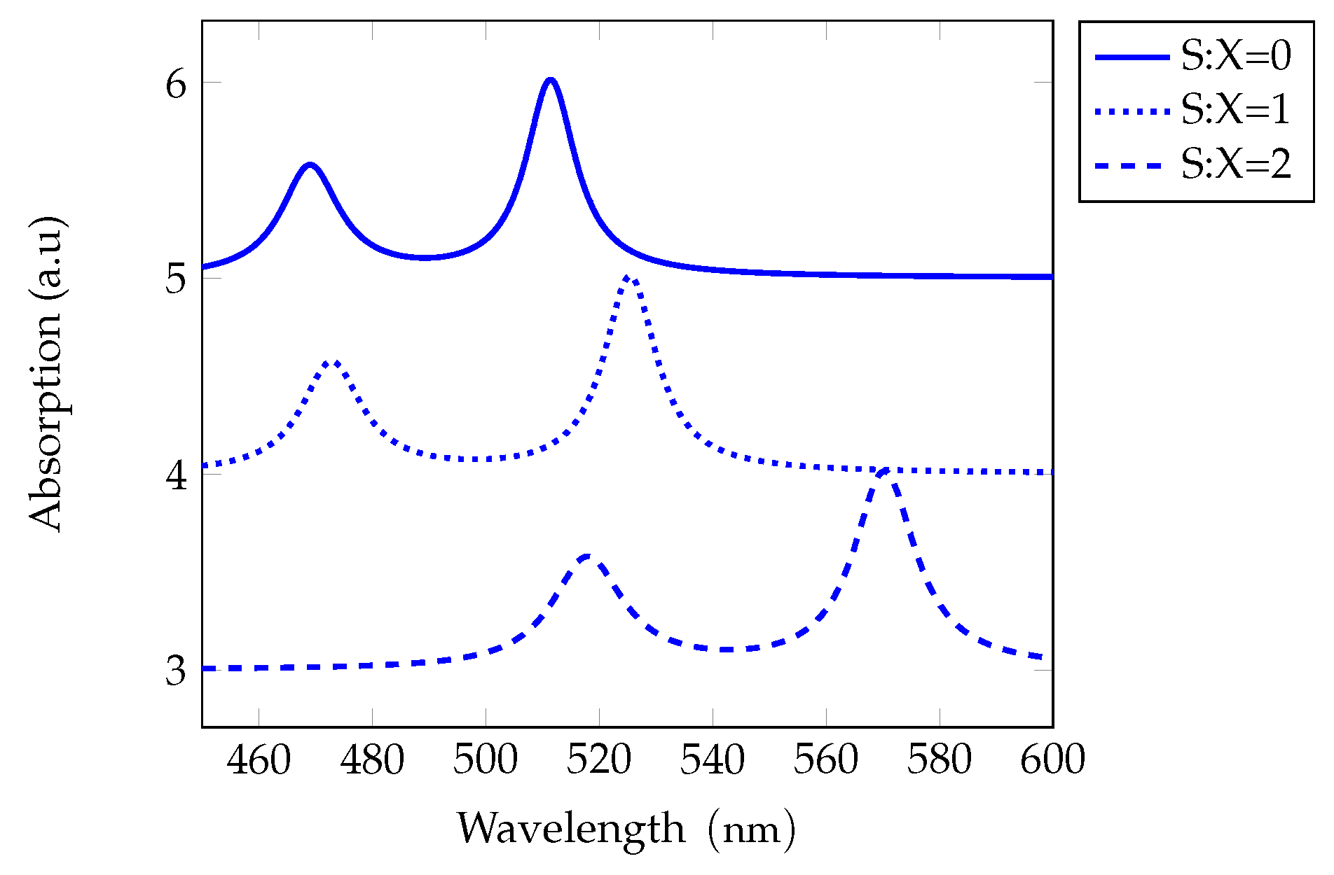
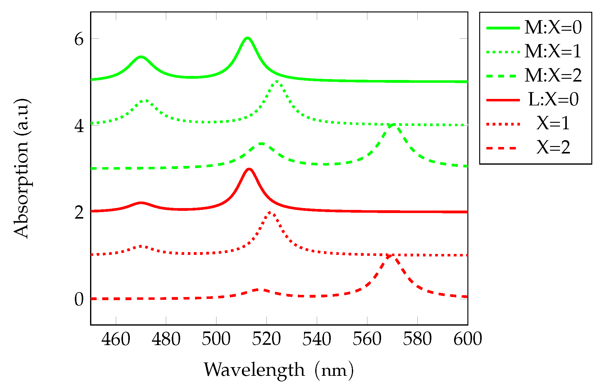
Figure 10.
Normalized absorption for the case ’Lateral Area’ at 273 K, for three values of the applied field in the case 4ML thickness and area (M="medium"), (L="large"), field strength in .
Figure 10.
Normalized absorption for the case ’Lateral Area’ at 273 K, for three values of the applied field in the case 4ML thickness and area (M="medium"), (L="large"), field strength in .
6. Quantum Confined Franz-Keldysh Effect
When the excitation energy exceeds the total confinement energy (including the energy gap), and an external electric field is applied parallel to the NPL plane, oscillations in the optical functions appear which, in the case of unbounded media, are known as the Franz-Keldysh effect (see, for example, [29]). For the unbounded media they have the form of outgoing waves, with variable periodicity and amplitudes (see, for example, [30,31]). The situation changes, when the medium, as considered here NPL, is finite. Instead of outgoing waves, standing waves appear, with periodicity and amplitude depending both on the applied field strength, and on the NPL size. This effect can be called Quantum Confined Franz-Keldysh effect (QCFKE). Such term appeared previously [32], but in the cited paper only a partial confinement was considered (QW), the field was applied in the z-direction, and the effect appears in the limits . The situation considered below is quite different, the confinement is applied in 3 direction, and the term Quantum Confined Franz-Keldysh effect seems to be justified. In the considered excitation region one can, in lowest approximation, neglect the e-h Coulomb interaction. Then the remaining terms in the Hamiltonian correspond to kinetic energies, and compose the total confinement. Therefore, to analyze the NPL’s QCFKE, we use the constitutive equation in the form
where
In the above equations the electric field F is parallel to the x-axis, and we retained the assumptions about the hole located in the NPL center. As in the case of unbounded media, the equation (40) can be solved by using appropriate Green’s function, which has the form
Here are the Airy functions ([28]), and the notation means , and . The confinement effect is included since
When the dipole density is defined, we obtain the NPL susceptibility in the form
The absorption coefficient is proportional to the imaginary part of the susceptibility. Its shape, showing Franz-Keldysh oscillations, is presented in Figure 11, for two values of the applied fields, and two lateral NPL dimensions. We notice the large dependence on the NPL both on the field strength, and on the size.
7. Conclusions
In this paper we have studied the electro-optical properties of CdSe NPLs with excitons, for various orientations of the applied static electric field. This properties, compared with analogous for bulk materials and QWs, show strong modifications, which are due to the total confinement of electrons and holes, with a resulting dependence of the spectra on NPLs sizes. Besides of various orientations, we have separately analyzed the two possibilities of the exciting wave energy, below and above the gap. For the energy below the gap and for both orientations of the field, we observe exciton resonances, shifted red (electric field parallel to the NPL plane), and shifted blue (electric field parallel to the z-axis). The latter effect is due to the lowering of the exciton binding energy, which prevails over the, also observed, quadratic Stark shift. In the case of the excitation energy exceeding the gap (enlarged by the confinement energy), we observe the Franz-Keldysh oscillations, with periodicity depending both on the applied field strength, and NPLs sizes. Thus, we have demonstrated that CdSe NPLs have an additional mechanism to control the exciton states not only by their thicknes (z-direction) and lateral size variation, but also by the strength and orientation of an applied constant electric field. It paves the way for construction of high sensitivity modulators, based on NPLs. The obtained results agree well with the available experimental results.
Funding
The authors have no funding to declare.
Data Availability Statement
The original contributions presented in this study are included in the article/supplementary material. Further inquiries can be directed to the corresponding author.
Conflicts of Interest
The authors declare no conflicts of interest and have no competing interests.
Appendix A. Calculations of Stark Shift and Oscillator Strengths for F‖z
For calculations of the Stark shift we have to specify the confinement parameters . They are related to the eigenvalues, which we identify with the eigenenergies for the vertical motion obtained in the case of dielectric confinement, and having the form
which give the confinement energy
with
where , and are the hydrogen Bohr energy and hydrogen Bohr radius, respectively. Using the value of , and the definitions
we obtain the confinement energy
where
with E given in meV and L in nm. By the relation
one obtains
The quantities are obtained by the relations
In the above calculations we have taken into account that the electron and hole effective masses given in Table 1 are in units of the free electron mass . Making use of the obtained expressions we arrive at the Stark shift
where
With regard to definitions (A1) and
we arrive at the Stark shift for heavy-hole and light-hole excitons in the form
where
and is the total exciton mass in the z-direction.
The oscillator strength is defined in terms of the function
which gives
Using the expressions for we arrive at
The final expression for the oscillator strength reads
Appendix B. Calculations of Stark Shift and Oscillator Strengths for F in NPL Plane
In the case of applied field parallel to the NPL plane, discussed in Sec. 5, one has to solve the 1-dimensional Schrödinger equation
with the confinement potential V defined in Eq. (37). Using scaled variables
we obtain equation
It has the form of the Whittaker equation (see Ref. [28])
with 2 linearly independent solutions , from which we choose the function finite at . It is related to the confluent hypergeometric function by the relation
The Eq. (A14) is a special case of Eq. (A15) for , thus the solution of (A14) reads
The eigenvalues will be obtained from the equation
Using the expansion of and retaining the terms at most quadratic in , we obtain the equation for eigenvalues
with , and the solutions
The equation defines the critical size , which means that positive solutions exist for . The above considered NPLs satisfy this condition.
Having calculated t, we obtain the eigenvalues by the equation
The quantity t also determines the eigenfunctions, having the form
where C is the normalization constant.
References
- Joo, J.;, Son, J.S.; Kwon, S.G.; Yu, J.H; and Hyeon, T. Low-temperature solution-phase synthesis of quantum well structured CdSe nanoribbons. J. Am. Chem. Soc. 2006, 128, 5632.
- Achtstein, A.W.; Schliwa, A.; Prudnikau, A.; Hardzei. M.; Artemyev, M.V.; Thomsen, C.; and Woggon, U. Electronic Structure and Exciton-Phonon Interaction in Two-Dimensional Colloidal CdSe Nanosheets. Nano Lett. 2012, 3151-7. doi: 10.1021/nl301071n. Epub 2012 May 29.
- Benchamekh, R.; Gippius, N.A.; Even, J.; Nestoklon, M.O.; Jancu, J.M.; Ithurria, S.; Dubertret, B.; Efros, A.L.; and Voisin, P. Tight-binding calculations of image-charge effects in colloidal nanoscale platelets of CdSe. Phys. Rev. B 2014, 89, 035307. [CrossRef]
- Zelewski, S.J.; Nawrot, K.C.; Żak, A.; Gładysiewicz, M.; Nyk, M.; and Kudrawiec, R. Exciton Binding Energy of Two-Dimensional Highly Luminescent Colloidal Nanostructures Determined from Combined Optical and Photoacoustic Spectroscopies. J. Phys. Chem. Lett. 2019, 10, 3459. doi: 10.1021/acs.jpclett.9b00591.
- Shornikova, E.V.; Yakovlev, D.R.; Gippius, N.A.; Qiang, G.; Dubertret, B., Khan, A.H.; Di Giacomo, A.; Moreells, I.; and Bayer, M. Exciton binding energy in CdSe nanoplatelets measured by one- and two-photon absorption. Nano Lett. 2021, 21, 10525. [CrossRef]
- Brumberg, A.; Harvey, S.M.; Philbin, J.P.; Diroll, T.; Lee, B.; Crooker, S.A.; Wasielewski, M.R; Rabani,E.; and Schaller, R.D. Determination of the In-Plane Exciton Radius in 2D CdSe Nanoplatelets via Magneto-optical Spectroscopy, ACS Nano 2019, 13, 8589. [CrossRef]
- Yu, J.; and Chen, R. Optical properties and applications of two-dimensional CdSe nanoplatelets. InfoMat 2020, 2, 905. DOI: 10.1002/inf2.12106.
- Dutta A.; Medda, A.; and Patra, A. Recent Advances and Perspectives on Colloidal Semiconductor Nanoplatelets for Optoelectronic Applications. The Journal of Physical Chemistry C 2021, 125, 20. [CrossRef]
- Geiregat, P.; Rodá, C.; Tanghe, I.; Singh, S.; Alessio Di Di Giacomo, A.; Lebrun, D.; Grimaldi, G.; Maes, J.; Van Thourhout, D.; Moreels, I.; Houtepen, A.J.; and Hens, Z. Localization-limited exciton oscillator strength in colloidal CdSe nanoplatelets revealed by the optically induced stark effect. Light: Science & Applications 2021, 10, 112. [CrossRef]
- Gonçalves, I.M.; Medda, A.; Bautista, J.E.Q.; Campos, C.L.A.V.; Ghosh, S.; Patra, A.; and Gomes, S.L.A. Saturable absorption and third-order nonlinear refraction of 2D CdSe nanoplatelets resonant with heavy-hole excitonic transitions. Appl. Phys. Lett. 2023, 123, 251108. [CrossRef]
- Akhmetova, A.; Kainarbay, A.; Daurenbekov, D.; Nurakhmetov, T.; Zhangylyssov, K.; and Yussupbekova, B. Effect of Nanoplatelets Thickness on Photoluminescent, Optical, and Electronic Properties of Synthesized CdTe Semiconductor Nanoplatelets. Crystals 2023, 13, 1450. [CrossRef]
- Koshkinbayev, Y.; Ospanova, A.; Akhmetova, A.; Nurakhmetov, T.; Kainarbay, A.; Zhangylyssov, K.; Dorofeev, S.; Vinokurov, A.; Bubenov, S.; and Daurenbekov, D. The Influence of Temperature and Stoichiometry on the Optical Properties of CdSe Nanomaterials 2024, 14(22), 1794; [CrossRef]
- Ngo, H.T. Optical and electronic properties of colloidal CdSe nanoplatelets and related heterostructures. Micro and nanotechnologies/Microelectronics. Université de Lille; Universiteit Gent 2024. ffNNT : 2024ULILN025.
- Czajkowski, G. Optical properties of excitons in CdSe nanoplatelets. J. Biomed. Res. Environ. Sci. 2026 Jan 08;7(1):19. Doi: 10.37871/jbres2230, also: arxiv 2025. arxiv.org/pdf/2511.02857.
- Silva, C.R. da;, Bechstedt, F.; Teles, L.K.; and Marques, M. Electronic and Optical Properties of highly Complex Ga2O3 Polymorphs using approximate quasiparticle DFT+A+1/2. 2024. [CrossRef]
- Grillo, S.; Cignarella , Ch.; Bechstedt, F.; Gori, P.; Palumno, M.; Campi, D.; Marzari, N.; and Pulci, O. Quasiparticle Effects and Strong Excitonic Features in Exfoliable 1D Semiconducting Materials, ACS Nano 2026, 20, 2664. [CrossRef]
- Capellini, G.; Furthmüller, J.; Bechstedt, F.; and Botti, S. Electronic and Optical Properties of Alkaline Earth Metal Fluoride Crystals with the Inclusion of Many-Body Effects: A Comparative Study on Rutile MgF2 and Cubic SrF2, 2023. Symmetry, 15,539. .https://doi:10.3390/sym15020539.
- Furthmüller, J.; Bechstedt, F.; Botti, S.; and Cappellini, G. Influence of spin-orbit interaction and self-consistency on quasiparticle electronic structure and exciton optical spectra beyond Tamm-Dancoff: The case of BaF2 and SrF2. Physical Review B 2025. 112, 195112. [CrossRef]
- Miller, D.A.B.; Chemla, D.S.; Damen, T.C.; Gossard, A.C.; Wiegmann, W.; Wood, T.H.; and Burrus, C.A. Band-Edge Electroabsorption in Quantum Well Structures: The Quantum-Confined Stark Effect. Phys. Rev. Lett. 1984, 53, 2173.
- Achtstein, A.W.; Prudnikau, A.V.; Ermolenko, M.; Gurinovich, L.I.; Gaponenko, S.V.; Woggon, U.; Baranov, A.V.; Leonov, M.Yu.; Rukhlenko, I.D.; Fedorov, A.V.; and Artemyev, M.V. Electroabsorption by 0D, 1D, and 2D Nanocrystals: A Comparative Study of CdSe Colloidal Quantum Dots, Nanorods, and Nanoplatelets. ACS Nano 2014. DOI: 101021/nn503745u.
- Ziemkiewicz, D.; Czajkowski, G.; Karpiński, K.; and Zielińska-Raczyńska, S. Electro-optical properties of excitons in Cu2O quantum wells. I. Discrete states. Phys. Rev. B 2021, 104, 075303.DOI: 10.1103/PhysRevB.104.075303.
- Baghdasaryan, D.A.; Harutyunyan, V.A.; and Sarkisyan, H.A. Linear and non-linear electrooptical transitions in CdSe nanoplatelets. Optical and Quantum Electronics 2024, 56,1221. [CrossRef]
- Rong, Y.; Huo, Y.; Fei, E.T.; Fiorentino, M.; Tan, M.R.T.; Ochalski, T.; Huyet, G.; Thylen, L.; Chacinski, M.; Kamins, T.I.; and Harries, J.S. High speed optical modulation in Ge quantum wells using quantum confined stark effect. Front. Optoelectron. 2012, 5,82. doi.org/10.1007/s12200-012-0194-9.
- Ziemkiewicz D.; Knez D.; Garcia, E.P.; Zielińska-Raczyńska, S.; Czajkowski, G.; Salandrino A.; Kharintsev. S.S.; Noskov, A.I.; Potma, E.O.; and Fishman, D.A. Two-Photon Absorption in Silicon Using Real Density Matrix Approach. Journ. Chem. Phys. 2024; 161: 144117. doi: 10.1063/5.0219329.
- Landau, L.D; and Lifshitz, E.M. Electrodynamics of Continuous Media, 2nd Ed. by E. M. Lifshitz and L. P. Pitaevskii. 1984, Pergamon Press, Oxford. ISBN 0-08-030276-9.
- Caicedo-Davila, S.; Caprioglio, P.; Lehmann, F.; Levcenco, S.; Stolterfoht, M.; Neher, D.; Kronik, L.; and Abou-Ras, D. Effects of Quantum and Dielectric Confinement on the Emission of Cs-Pb-Br Composites, Adv. Func. Mater. 2023,33, 2305240. [CrossRef]
- Kurtina, D.A.; Long, H.; Chang, S.; Vasiliev, R.B. Solvent effect on chiroptical properties of chiral atomically thin CdSe nanoplatelets capped with enantiomeric ligands. Optical Mat. 2025, 158, 116483. [CrossRef]
- In Handbook of Mathematical Functions; Abramowitz, M., and Stegun, I., eds. Handbook of Mathematical Functions. 1964, Dover Publications, ISBN 0-486-61272-4. New York, US. http://www.ams.org/notices/201107/rtx110700905p.pdf,.
- Kalt, H.; and Klingshirn, C.F. Semiconductor optics. 2019, Springer Nature, Cham, Switzerland. [CrossRef]
- Zielińska-Raczyńska, S.; Ziemkiewicz, D.; and Czajkowski, G. Electro-optical properties of Cu2O for P excitons in the regime of Franz-Keldysh oscillations. Phys. Rev. B 2018, 97, 165205.DOI: 10.1103/PhysRevB.97.165205.
- Ziemkiewicz, D.; Czajkowski, G.; Karpiński, K.; and Zielińska-Raczyńska, S. Electro-optical properties of excitons in Cu2O quantum wells. II.Continuum states II. Phys. Rev. B 2021, 104, 075304. DOI: 10.1103/PhysRevB.104.075304.
- Miller, D.A.B.; Chemla, D.S.; and Schmitt-Rink, S. Relation between electroabsorption in bulk semiconductors and in quantum wells: The quantum-confined Franz-Keldysh effect. Phys. Rev. B 1986, 33, 6976. [CrossRef]
Figure 1.
Schematic picture of a nanoplatelet. Two discussed applied field orientations are indicated.
Figure 1.
Schematic picture of a nanoplatelet. Two discussed applied field orientations are indicated.
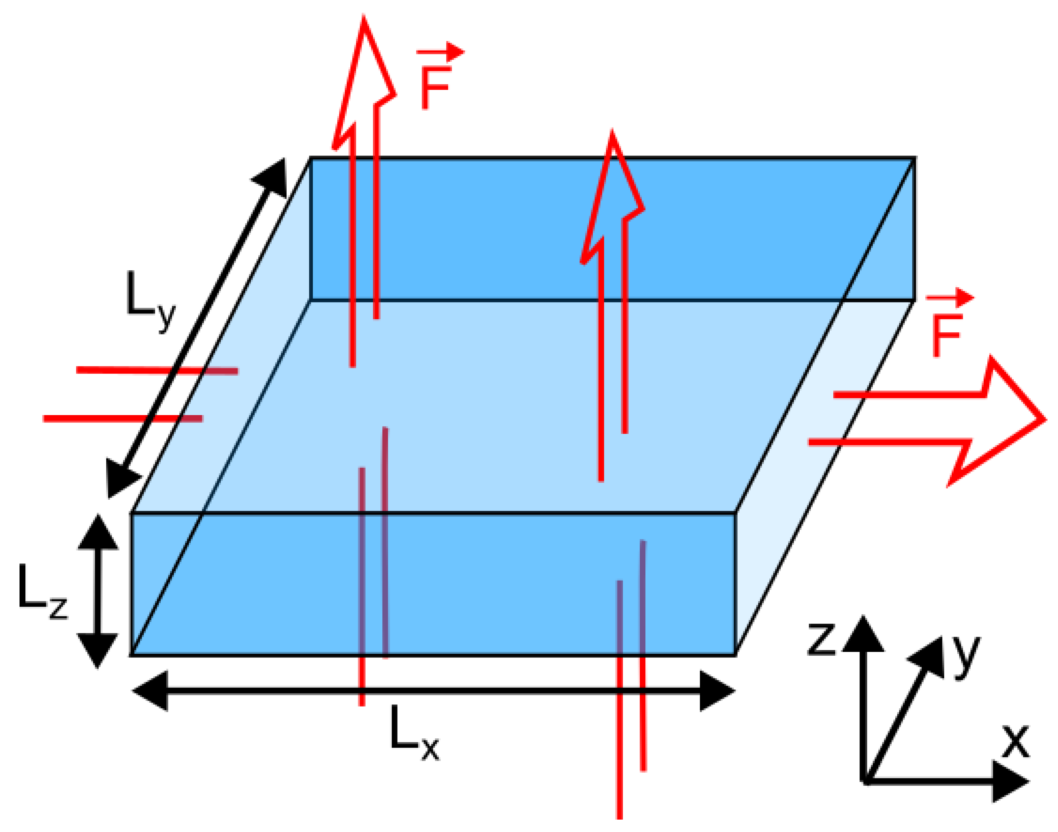
Figure 2.
Stark shift for CdSe NPLs and heavy-hole excitons (solid lines), and light-hole excitons (dotted lines).
Figure 2.
Stark shift for CdSe NPLs and heavy-hole excitons (solid lines), and light-hole excitons (dotted lines).
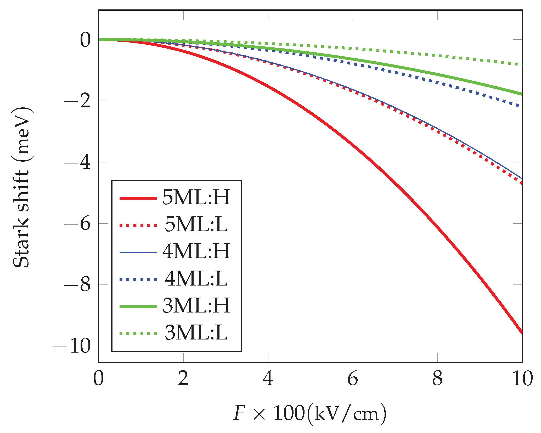
Figure 7.
Stark shift for CdSe NPLs and heavy-hole excitons, for
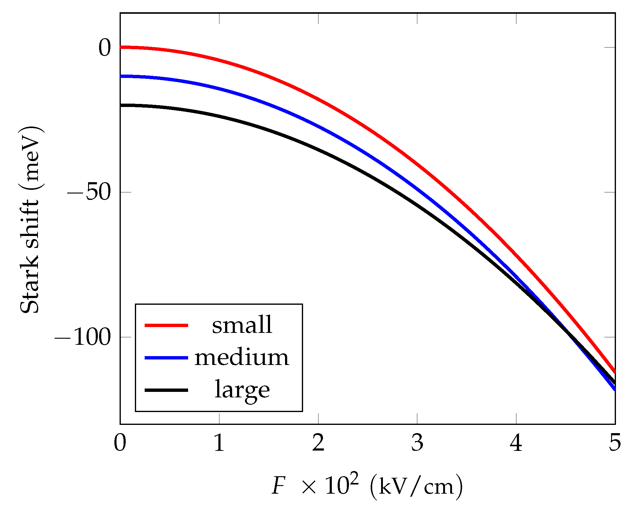
Figure 8.
The shift in the heavy-hole exciton energy as the lateral size of the NPL increases, for .
Figure 8.
The shift in the heavy-hole exciton energy as the lateral size of the NPL increases, for .
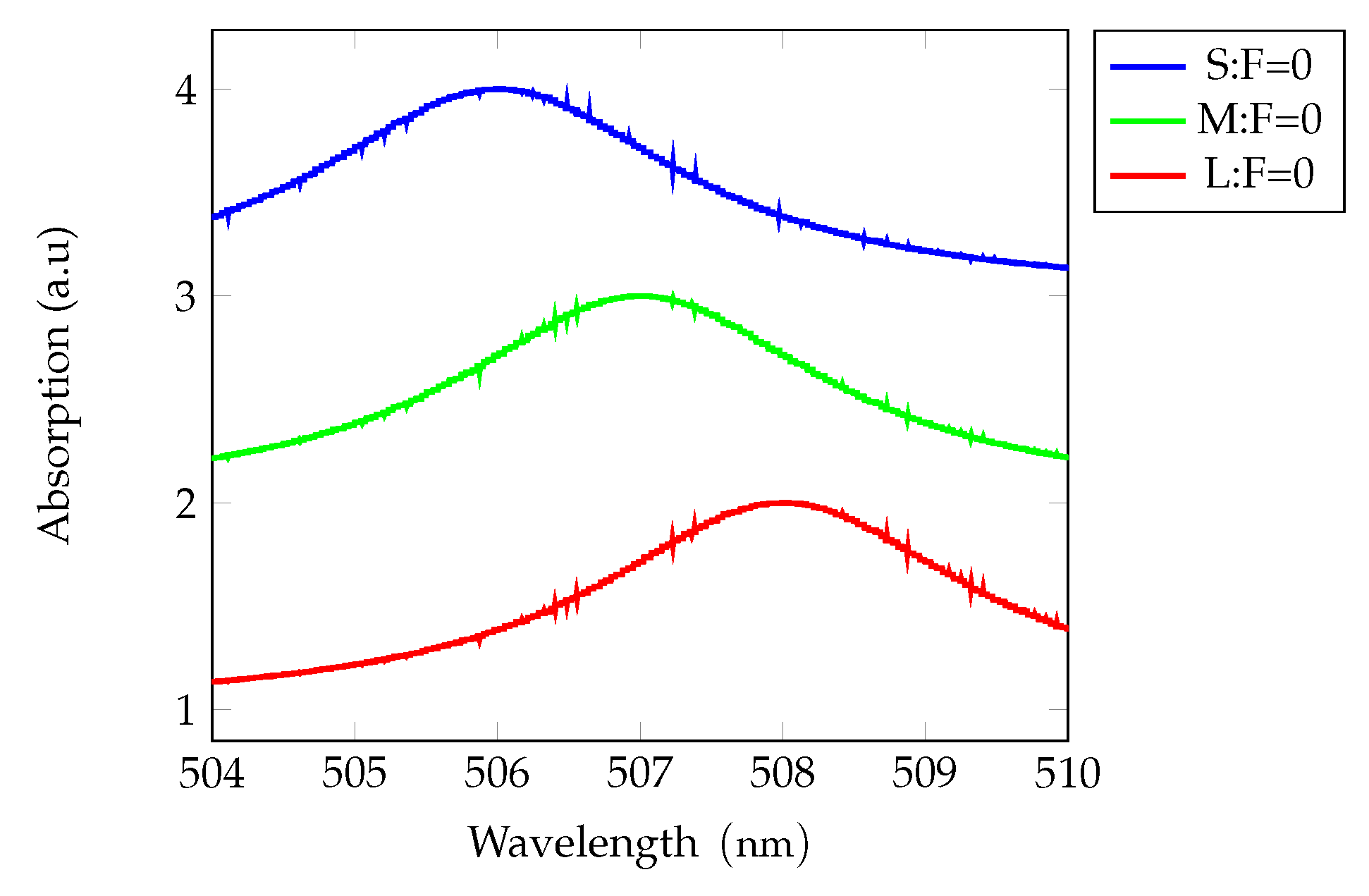
Figure 11.
Absorption, .
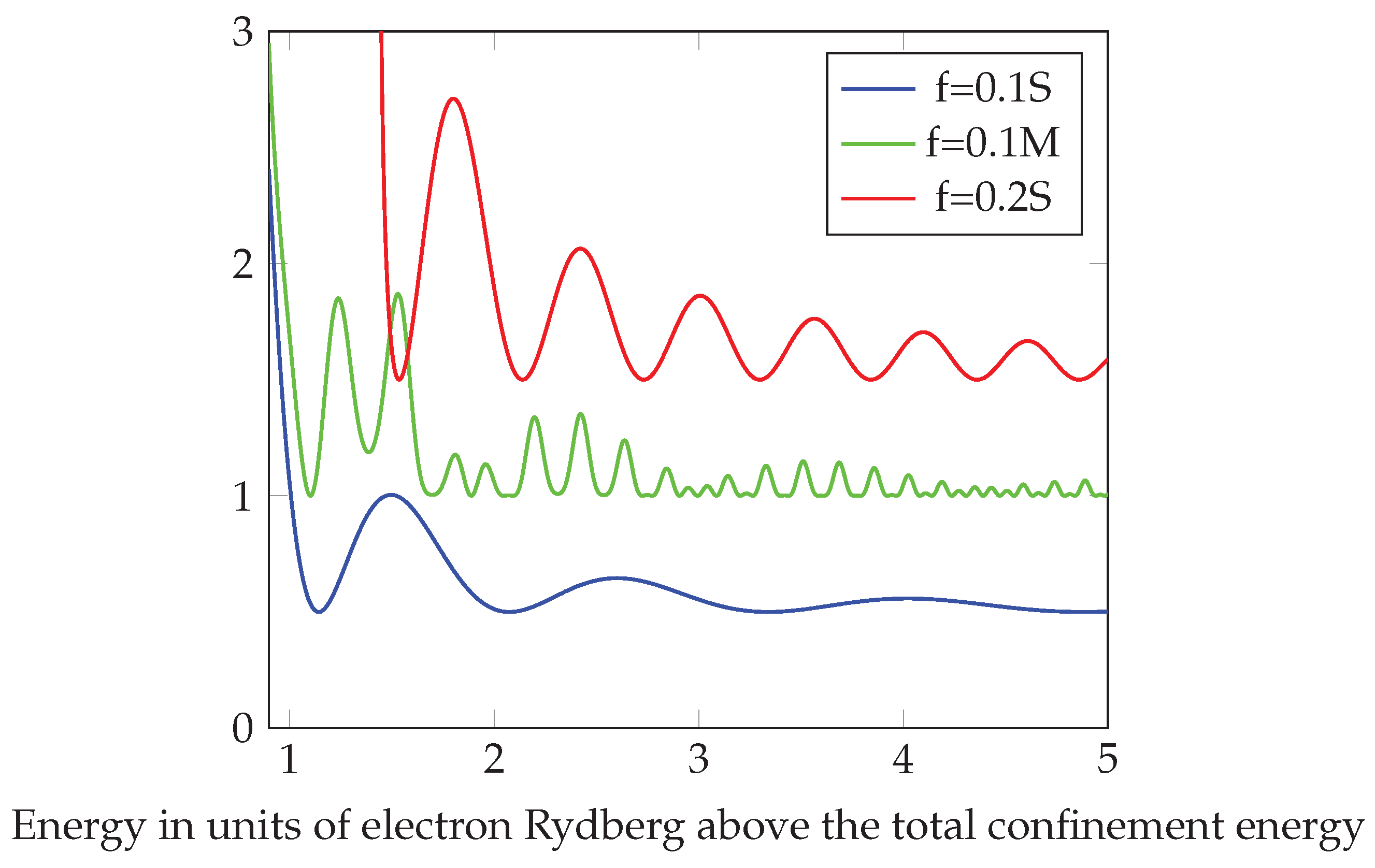
Table 3.
Parameters for calculating the Stark shift, excitonic resonance energies vs applied field strength and lateral area, field strength in kV/cm, , energies in meV, wavelengths in nm, oscillator strength to be multiplied by .
Table 3.
Parameters for calculating the Stark shift, excitonic resonance energies vs applied field strength and lateral area, field strength in kV/cm, , energies in meV, wavelengths in nm, oscillator strength to be multiplied by .
| Param. | |||
| 3.283 | 3.22 | 3.03 | |
| 10.78 | 10.375 | 9.22 | |
| 1.89 | 1.82 | 1.62 | |
| 4.72 | 4.55 | 4.04 | |
| 4.5 | 4.33 | 3.85 | |
| 227.9 | 226.38 | 281.76 | |
| 2450.166 | 2448 | 2441 | |
| 506 | 506.54 | 508 | |
| 2670.166 | 2668 | 2661 | |
| 464.39 | 464.77 | 466 | |
| 243.52 | 243.04 | 241.67 | |
| 2408.3 | 2410.5 | 2417.36 | |
| 514.88 | 514.41 | 512.95 | |
| 2628.3 | 2630.5 | 2637.6 | |
| 471.8 | 471.4 | 470.12 | |
| 288.15 | 287.46 | 278.72 | |
| 2360.2 | 2362.84 | 2377.42 | |
| 525.36 | 524.79 | 521.57 | |
| 2580 | 2582.84 | 2597.42 | |
| 480.6 | 480.1 | 477.4 | |
| 478.49 | 481.63 | 477.2 | |
| 2174.45 | 2173 | 2177.42 | |
| 570.25 | 570.63 | 569.48 | |
| 2394.45 | 2393.0 | 2397.4 | |
| 517.86 | 518.18 | 517.22 |
Disclaimer/Publisher’s Note: The statements, opinions and data contained in all publications are solely those of the individual author(s) and contributor(s) and not of MDPI and/or the editor(s). MDPI and/or the editor(s) disclaim responsibility for any injury to people or property resulting from any ideas, methods, instructions or products referred to in the content. |
© 2026 by the author. Licensee MDPI, Basel, Switzerland. This article is an open access article distributed under the terms and conditions of the Creative Commons Attribution (CC BY) license.
Copyright: This open access article is published under a Creative Commons CC BY 4.0 license, which permit the free download, distribution, and reuse, provided that the author and preprint are cited in any reuse.


