
Submitted:
27 January 2026
Posted:
27 January 2026
You are already at the latest version
Abstract
Aided by quantum sources, quantum metrology helps enhance measurement precision. Here, we construct a theoretical model for quantum imaging based on squeezed states and present the corresponding numerical results. Through discretization and quantum Fisher information theory, we investigate the two-point resolution and spatial multi-parameter estimation of optical fields with unknown spatial distributions. We calculate and compare imaging results based on squeezed vacuum states, coherent states, and squeezed coherent states; our results show that squeezed coherent states yield greater quantum Fisher information, which can effectively improve imaging quality. In addition, we analyze the influence of imaging basis functions, degree of squeezing, quantum correlations, and other factors on imaging performance. The proposed quantum imaging model and computational method can be extended to more complex scenarios, such as multi-mode squeezed-state imaging schemes and incoherent imaging systems. In the future, it is expected to find applications in practical imaging systems, including Raman microscopy and stimulated Brillouin scattering imaging.
Keywords:
squeezed state
; quantum imaging
; quantum Fisher information
1. Introduction
Optical imaging technology plays a crucial role in humanity’s exploration of the unknown world. However, the resolution of traditional imaging systems is limited by the Rayleigh diffraction limit. Based on quantum Fisher information theory, Tsang et al. were the first to investigate the fundamental limits of imaging resolution and the method for achieving two-point super-resolution imaging [1]. Subsequently, research on super-resolution imaging grounded in quantum information theory has been extensively developed, evolving from initial one-dimensional two-point imaging to the estimation of multiple points and three-dimensional imaging [2,3,4]. This research has further extended to practical imaging scenarios involving factors such as detection noise and mode crosstalk [5,6,7]. Currently, super-resolution quantum imaging has become a focal point of research. Nevertheless, existing studies remain primarily concentrated in the field of imaging with incoherent thermal light sources.
Squeezed states serve as a crucial quantum resource for enhancing the precision of quantum measurements [8], exemplified by their application in gravitational-wave laser interferometers [9]. With the continuous advancement of research, the application of squeezed states in quantum imaging has emerged as a new and prominent research direction. This is evidenced by studies in areas such as Raman microscopy imaging [10,11,12] and stimulated Brillouin scattering imaging [13]. These studies demonstrate that quantum imaging based on squeezed states can effectively overcome the shot noise limit and improve imaging quality.
Can squeezed states enable quantum imaging that simultaneously overcomes both the shot noise limit and the Rayleigh diffraction limit? Mikhail I. Kolobov et al. theoretically explored quantum imaging based on spatially multimode squeezed vacuum states [14]. Their results indicate that squeezed states can achieve super-resolution quantum imaging surpassing the shot noise limit. However, they did not provide the ultimate quantum theoretical limit for such imaging. Giacomo Sorelli et al. [15] investigated the super-resolution problem for point sources using squeezed states based on quantum Fisher information theory and derived a quantum limit for resolution. Nevertheless, their system model is relatively simple and cannot be readily extended to the study of arbitrary images. Therefore, how to establish a comprehensive imaging theoretical model based on squeezed states and conduct research on super-resolution imaging utilizing squeezed states remains an open and pressing issue to be addressed.
To address the aforementioned issues related to super-resolution imaging based on squeezed states, this paper constructs a corresponding imaging theory model and presents numerical calculation results. By employing discretization and quantum Fisher information theory, the problem of two-point resolution is investigated. The correctness of the established model is verified through comparison with results from existing literature. Building upon this theoretical model, the paper further explores the problem of spatial multi-parameter estimation in imaging for light fields with arbitrary spatial distributions, demonstrating the advantages of squeezed coherent states in quantum imaging. This quantum imaging model and its computational methodology can be extended to more complex scenarios, such as imaging schemes based on multimode squeezed states, and even to incoherent imaging systems [16]. It thus lays a theoretical foundation for future experimental research on super-resolution imaging utilizing squeezed states.
2. Theoretical Methods
2.1. Description of the Imaging System
We consider a simple imaging system as shown in Figure 1. The multimode optical field at the object plane, represented by , is composed of a finite number of modes . This field corresponds to the optical modes excited at the object plane (typically resulting from the reflection or transmission of an illumination source), where denotes the annihilation operators of the optical field, and represents the corresponding spatial modes of the field. It carries the desired complex amplitude distribution information, which is the target to be reconstructed from the measurement results. In addition to , the vacuum field is also present at the object plane. The complete optical field at the object plane, is the superposition of the two. In our imaging model, is expanded using a set of modes as , where the relationship between and is given by
The expression refers to Appendix A. For scalar, quasi-monochromatic classical imaging problems, the propagation of the optical field’s complex amplitude from the object plane to the image plane is regarded as the action of an integral operator with the amplitude point spread function as its kernel on , yielding the optical field at the image plane.
Where represents the distribution area of the optical field. The quantum version of this form was provided by Jeffrey H. Shapiro [17]. Through singular value decomposition, the amplitude point spread function can be expressed as
Then, the diffraction process can be described as a transformation from the vector of annihilation operators corresponding to the modes to the vector of annihilation operators corresponding to the modes , given by , where
Where represents the vacuum state introduced due to diffraction losses. In practical computations, the sets and cannot be obtained directly. To perform the singular value decomposition, we first need to select a known set of basis functions for the object plane and image plane, and , and express in matrix form. Based on the calculation results, we then reselect and into the desired form. A suitable choice is the rectangular function basis. For our one-dimensional problem, the rectangular function basis is defined as
Here, is the width of the rectangle. As , we have
Its core advantage lies in enabling efficient inner product operations to avoid numerical integration, thereby improving computational efficiency. We first expand using and to obtain the matrix
Performing a truncated singular value decomposition on it, we obtain and discard the smaller singular values. The basis functions corresponding to the right singular vectors are approximated as , where represents the matrix elements of U. At this point, the corresponding annihilation operator vector has a lower dimensionality but contains the vast majority of the information from the image plane optical field. We use as the basis functions for expanding the object plane field to reduce the computational complexity of projection operations. The corresponding annihilation operator vector is . The image plane basis functions are expanded using to reduce the scale of the output information. The diffraction process is then expressed as the transformation from the annihilation operator vector corresponding to to , given by , where
Here, represents the vacuum state introduced due to losses (see Appendix A). The optical field at the image plane is obtained as . The overall transformation from the source field to the image plane field is described as follows.
2.2. Gaussian States in Linear Systems
In quantum optics, the quadrature amplitude operator and quadrature phase operator of an optical field are defined through the annihilation operator as and . The operator vector for a multimode Gaussian state is defined as . An important property of Gaussian states is that all statistical moments of the probability distributions for measurements of their quadrature amplitudes and phases can be completely described by their expectation value and covariance matrix . Therefore, these contain all the statistical information of the Gaussian state [18]. For a transformation
where X represents the transformation acting on the non-vacuum input , and Y is the transformation acting on the vacuum input. The following relationships hold:
where ⊗ denotes the Kronecker product. Both and can be expressed in terms of , , and :
where I denotes the identity matrix. Moreover, Equation (14) is invertible; its inverse operation is provided in Appendix B. Therefore, for a multi-mode Gaussian state, the calculation proceeds as follows: first, transform the input state’s and into , and using the inverse of Equation (14). Next, compute the output state’s , and via Equation (13). Finally, convert these results into and using Equation (14). In this process, the calculations require only the classical transformation X from Equation (13), with no term involved, thereby simplifying the analysis. For more complex systems, the overall transformation can be constructed through matrix multiplication or direct sums of multiple X matrices, thereby optimizing the computational cost.
2.3. Quantum Fisher Information for Gaussian States
The quantum Fisher information (QFI), denoted as F, is a physical quantity that quantifies the achievable precision for parameter estimation given a specific quantum state and measurement problem. It yields the quantum Cramér-Rao bound (QCRB) [18], (where N is the number of repetitions of the experiment) which represents the lower bound on the variance of an unbiased estimator for a given probe state. Consider a prepared probe state described by the density matrix . After interacting with the target of interest, the probe state evolves into , which now encodes information about the parameter t. The symmetric logarithmic derivative (SLD) operator , required for computing the QFI, can then be defined and solved via the Lyapunov equation:
This leads to the QFI . For multi-parameter estimation problems [19], the quantum Fisher information is generalized to the quantum Fisher information matrix (QFIM), with the corresponding QCRB expressed as a matrix inequality. Specifically, let the -dimensional parameter vector to be estimated be . Then the covariance matrix of satisfies
Generally, calculating the QFIM is quite complex. For scenarios where information is encoded into Gaussian states, Rosanna Nichols et al. [19] proposed an efficient and precise computational method that determines the QFIM based on the expectation values and covariance matrix. The matrix elements of the QFIM are given by:
where S and are derived from the Williamson decomposition of the covariance matrix .
where , S belongs to the real symplectic group , and is the symplectic structure matrix. is a block matrix composed of blocks, where all blocks are zero matrices except the block indexed by . The block labeled , denoted as , takes different forms depending on l: , , , .
For high-dimensional covariance matrices, conventional methods cannot directly yield a valid Williamson decomposition and instead only provide constraints on the solution [18,20]. Here, we refer to the work of Martin Houdede et al. [21], which presents a robust and accurate numerical method to achieve this decomposition. The details are provided in Appendix C.
Therefore, as illustrated in the Figure 2, the method for analyzing the imaging process is as follows:
- 1.
- Determine the amplitude point spread function based on the actual imaging system.
- 2.
- Discretize using and .
- 3.
- Obtain via truncated singular value decomposition.
- 4.
- Determine based on and .
The algorithm for calculating the QFIM is:
- 1.
- Input the parameter-dependent functions: , , and the transformation matrix , along with the parameter value .
- 2.
- Calculate , , and using the inverse of Equation (14).
- 3.
- Compute , , and via Equation (13).
- 4.
- Determine and using Equation (14).
- 5.
- Compute the partial derivatives and .
- 6.
- Assign the value to the parameter and perform the Williamson decomposition on to obtain , , and the symplectic eigenvalues using the method described in Appendix C.
- 7.
- Calculate and return the QFIM based on Equation (17).
Based on this framework, it is possible to automatically and rapidly compute the QFIM corresponding to any finite-dimensional parameter vector. Furthermore, by increasing the numerical precision and modeling accuracy, any desired finite computational precision can be achieved. In terms of describing interactions, compared to methods such as Gaussian channels [19] or symplectic transformations [18], this approach is not compatible with nonlinear processes like squeezing transformations. However, it offers advantages including convenient analysis, the ability to quickly construct composite maps via matrix multiplication and direct sums, efficient use of computational memory, and adaptability to cases where the numbers of input and output modes are unequal. Regarding the computation of the QFIM, this method integrates two efficient algorithms to achieve fast calculation of the matrix for multi-mode Gaussian states.
3. Application
3.1. Two-Point Resolution
Giacomo Sorelli et al. [15] discussed a two-dimensional imaging problem—the resolution of two point sources. The scenario involves two point-like emitters in the object plane, each in a Gaussian state. After passing through an imaging system described by a Gaussian point spread function, the light reaches the image plane, where the task is to estimate the separation distance between the two points using the imaging apparatus. Let the amplitude point spread function from object plane coordinates to image plane coordinates be
The object plane contains two point-like squeezed light sources located at and , respectively. The objective is to estimate their separation distance s. Since only the two points on the x-axis are considered, the problem can be decoupled as , where
is the normalized amplitude point spread function. With reference to the method of Giacomo Sorelli et al. [15], we calculated the QFI for the separation distance s between two point sources and (Note: A point source is described by a Dirac function, which is not square-integrable. Its handling is detailed in Appendix D). The calculation was performed for two thermal states, each with a mean photon number .
coherent states
squeezed vacuum states
squeezed coherent states , where ,
For the numerical calculations, we set the parameters as follows: The amplitude point spread function is given by with and the transmission coefficient . Correspondingly, the basis function width is set to . The basis functions at the object plane cover a range of width , and those at the image plane cover a range of width . After performing the singular value decomposition, the largest singular value is . The smallest singular value retained is the 20th one, with . In the computation process, the partial derivatives in Equation (17) are approximated using the central difference formula, , with a step size of .
Under this parameter configuration, the QFI for the two-point separation is calculated and plotted as a connected curve, with the results shown in the upper panel of Figure 3. For each calculated data point, the QFI per effective photon , obtained using the method from reference [15] (denoted as ) and that from our proposed method (denoted as ) are compared. The relative deviation is illustrated in the lower panel of Figure 3.
Under this parameter configuration, the discrepancy between the two methods is , thereby validating the correctness of our approach using existing results. For the two-point resolution problem, the estimation precision for a coherent state exhibits different curves depending on the relative phase between the two light sources. For estimating small separations , the coherent state achieves optimal precision when the relative phase is , and it reaches a higher precision limit compared to the case when , demonstrating a super-resolution phenomenon. This result is close to the upper bound of QFI given by Cosmo Lupo et al. [5]. For the squeezed vacuum state, it shows no advantage over the coherent state in the region of small, which is of primary interest. Building upon the work in reference [15], we consider coupling the optimal coherent state with a squeezed vacuum state to form a squeezed coherent state. By suppressing its displacement fluctuations, the precision can be further enhanced, surpassing the shot noise level.
3.2. Spatial Multi-Parameter Estimation of Optical Fields
To extend imaging from the two-point problem to broader quantum imaging applications, we now investigate the estimation of the unknown spatial distribution of an optical field. An optical field with a specific profile, after passing through an imaging system, forms a distorted spot on the image plane. Our task is to estimate the spatial distribution of the optical field at the object plane based on the field measured at the image plane.
Consider an optical field with an unknown spatial profile, represented by . The function is expanded using a set of basis functions
where the expansion coefficients are our estimation targets. Together with the known basis functions , they determine the characteristics of . We consider three schemes for mode expansion using and compare them. The first is the Hermite-Gaussian mode, commonly used in quantum optics and laser physics: . The second is a typical basis function on a closed interval, the Legendre polynomials: . The third is obtained from the singular value decomposition of the amplitude point spread function , giving the right singular vectors: .
We choose a representative and intuitive hypothetical field distribution for : , where is a normalization constant. Its profile is shown in Figure 4 (a). We consider reconstructing using the first 6 modes of the three aforementioned schemes. All three can achieve reconstruction with high accuracy; therefore, neglecting the influence of higher-order modes, we calculate the QFIM per average photon number for the parameter vector .
Our parameter settings are as follows: the basis function width is , , and correspondingly . For the amplitude point spread function, and the transmission coefficient is (chosen to avoid singular values greater than 1, which would cause model failure). After singular value decomposition, the largest singular value is . The smallest singular value retained is the 15th one, with . The step size for the central difference approximation is .
Under the three basis function schemes, the QFIM per average photon number , yielded by the coherent state is shown in Figure 4, respectively.
Furthermore, we calculated the diagonal elements of the QCRB for the three basis function schemes and compared them with the results obtained from the right singular vectors. This comparison reveals that the QCRB provided by the right singular vector basis expansion is optimal for every parameter’s precision lower bound. This conclusion serves as a verification, using quantum estimation theory, of a classical optics finding [22]. Additionally, after testing with various field profiles, we found that these computational results are independent of the specific values of the parameter vector and are general in nature.
Next, we consider further enhancing the estimation precision for the expansion coefficients within the framework of the right singular vector basis. We note that a bright squeezed coherent state , where the displacement direction aligns with the squeezing direction, can effectively improve estimation accuracy. The average photon number of a squeezed coherent state is given by . Considering practical experimental constraints, the coherent-part mean photon number is relatively easy to prepare. However, the squeezed-part mean photon number is typically limited to a smaller mean photon number due to technical challenges. Here, we focus on the scenario where .
Unlike the classical case, when the bright squeezed coherent state is used as the probe state,
the calculated QFIM becomes non-diagonal. This is because, as a non-classical optical field, the squeezed state exhibits quantum correlations between photons in different modes . However, the diagonal elements of are significantly reduced, and the matrix remains approximately diagonal. Its off-diagonal elements are of the same order of magnitude or one order smaller than the smallest diagonal element, , yet are numerically significantly smaller than . Thus, overall, the squeezed coherent state provides an improvement in precision.
Under the premise that , we fixed the squeezed-part mean photon number to a fixed value and incrementally increased the total photon number to calculate the QFIM. The observed trend in its values demonstrates an improvement characterized by a specific coefficient relative to the standard quantum limit. Keeping the total photon number fixed at while varying , we found that the degree of improvement offered by the squeezed coherent state is jointly influenced by the values of the parameter vector and the singular values . We investigated the enhancement effect provided by the squeezed-part mean photon number under two different optical field energy distributions.
From Figure 5, it can be observed that the performance gain offered by the squeezed state over the coherent state is more pronounced for larger singular values , and larger coefficients . However, as the mean photon number in the squeezed-part increases, the marginal improvement in estimation precision achieved by further squeezing gradually diminishes.
In general, for coherent imaging, one must account for not only the intensity distribution but also the phase distribution of the optical field, both of which are crucial. Therefore, we consider a more general complex-valued scenario represented by the parameter set . Using the same imaging system and parameters, with the right singular vectors as the basis set for calculation, we obtained the following result:
For the coherent state, the QCRB remains diagonal. This indicates that when using classical resources, there exists no statistical correlation among the parameters .
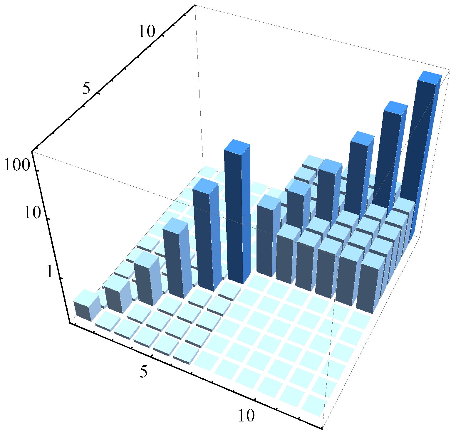
For the squeezed coherent state, as shown in Figure 6, is a block-diagonal matrix. Quantum entanglement induces statistical correlations among the estimates for different amplitude distribution parameters and among the estimates for different phase parameters . However, no statistical correlation exists between the amplitude part and the phase part. Therefore, estimating the amplitude distribution and the phase distribution independently is optimal. However, due to the presence of correlations within each part, performing separate measurements on individual modes cannot extract complete quantum information. Consequently, the optimal measurement scheme that approaches the QCRB requires a specific form of joint measurement.
Furthermore, we also examined the achievable estimation precision for the phase distribution of the optical field. Limited by the number-phase uncertainty relation, the estimation precision for the amplitude distribution and the phase distribution cannot be enhanced simultaneously. Employing a phase-squeezed state can likewise improve the estimation of the phase distribution. The degree of this improvement is influenced by the singular values and the energy distribution of the optical field, exhibiting a trend similar to that observed for amplitude estimation.
Overall, for estimating the spatial distribution of in the unknown optical field , we transform the problem into a multi-parameter estimation task via the basis function expansion method. Among various expansion schemes, we confirm that using the right singular vectors as the basis functions achieves the optimal estimation precision.
Compared to the coherent state, the squeezed coherent state can further enhance the estimation precision for either the amplitude or the phase of the basis function expansion coefficients. The degree of this improvement increases with larger singular values , larger expansion coefficients , and a higher mean photon number in the squeezed-part .
Due to the quantum correlations among different modes, when utilizing a squeezed coherent state as the resource, estimating the amplitude or phase distribution parameters requires a joint measurement scheme to approach the QCRB.
4. Conclusions
This paper establishes an imaging theoretical model based on Gaussian states and a corresponding method for calculating the quantum Fisher information of an imaging system, investigating quantum imaging problems utilizing squeezed states. First, we investigated the two-point imaging problem. Consistent with existing literature, our study confirms that a squeezed vacuum state does not enhance coherent imaging quality. We further explored two-point imaging with a squeezed coherent state, and the results demonstrate its superior performance compared to both thermal and coherent states.
Subsequently, we extended the research to the imaging of general patterns, specifically addressing the multi-parameter estimation problem for the spatial distribution features of an image. The squeezed coherent state exhibits the potential to surpass the shot noise limit in multi-parameter estimation, with the optical field’s energy distribution and system losses identified as key factors influencing the degree of squeezing-enhanced performance. However, due to potential quantum correlations among different parameters, separate measurements targeting individual modes are insufficient for extracting complete quantum information. Therefore, realizing the quantum Cramér-Rao bound by devising optimal experimental measurement schemes, and further proceeding to a comprehensive evaluation of the quantum enhancement effect, remain important open questions for future exploration.
The quantum imaging model and computational methodology presented here can be extended to more complex scenarios, such as imaging schemes based on multimode squeezed states, as well as to incoherent imaging systems [16]. Furthermore, it paves the way for exploring applications in practical imaging contexts, including Raman microscopy imaging [10,11,12] and stimulated Brillouin scattering imaging [13].
Author Contributions
Conceptualization, C. P. and K. L.; methodology, C. P.; software, C. P. and Y. X.; validation, C. P. and Y. X.; formal analysis, C. P.; investigation, K. L. and C. P.; data curation, C. P. and Y. X.; writing—original draft preparation, C. P.; writing—review and editing, C. P., Y. X. and K. L.; visualization, C. P. and Y. X.; supervision, K. L.; project administration, K. L.; funding acquisition, K. L. All authors have read and agreed to the published version of the manuscript.
Funding
This research was funded by National Natural Science Foundation of China(NSFC) (62575161); The central government guides local funds for science and technology development (YDZJSX20231A001).
Informed Consent Statement
Not applicable.
Data Availability Statement
Data are contained within the article.
Conflicts of Interest
The authors declare no conflicts of interest.
Appendix A. Multimode Bosonic Fields in Linear Systems
For the propagation of multimode bosonic fields, we can start from a simple model, first considering the beam splitter model in quantum optics:
where and are the annihilation operators of the optical fields at the input ports, and , are the annihilation operators at the output ports. The parameter represents the transmission efficiency from to . By placing multiple such beam splitters in parallel with their ports independent, we have:
Let the non-vacuum field operators among the form the vector . The output fields of interest among the form the vector . The corresponding vacuum fields among the that couple into form the vector . Neglecting the unobserved output fields , the transformation can be written as:
When , is an matrix
is an matrix
When , some of the are not coupled into the output. Here, and are diagonal matrices composed of selected elements and , respectively. Introducing unitary transformations U and V, and setting , , substituting these into (A3) yields:
where and . This describes the process by which a multimode bosonic field evolves into after coupling with a multimode vacuum field in a lossy linear system. Here, X corresponds to the classical transformation of the linear system, and is its singular value decomposition. Since Y can be derived from the singular value decomposition of X, the classical transformation X completely characterizes the quantum behavior of the bosonic field within the linear system. In optical systems, X corresponds to the transmission matrix in classical optics.
Appendix B. Statistical Moments and Normal-Ordered Operator Expectation Values
Given , and substituting the definitions and , we obtain
According to the definition , expanding the calculation shows that the covariance matrix is a block matrix composed of submatrices. The block at the j-th row and k-th column is:
From the relations and , and substituting the canonical commutation relation into Eq. (A8), we obtain after simplification:
Writing Equation (A9) in matrix form yields the expression for the covariance matrix in Equation (14).
Defining matrices , , , whose elements satisfy the corresponding relationships:
Appendix C. Technical Details of the Williamson Decomposition
The work by Martin Houdede et al. [21] presents a method for computing the Williamson decomposition for the symplectic structure matrix (where O is the zero matrix). We have adapted this method to obtain the Williamson decomposition for the symplectic structure matrix . The core of this algorithm transforms the Williamson decomposition problem into a Schur decomposition problem, for which efficient and robust built-in algorithms are readily available in major mathematical software packages.The complete Williamson decomposition calculation procedure is shown in Figure A1.
Figure A1.
The computational workflow for the Williamson decomposition.
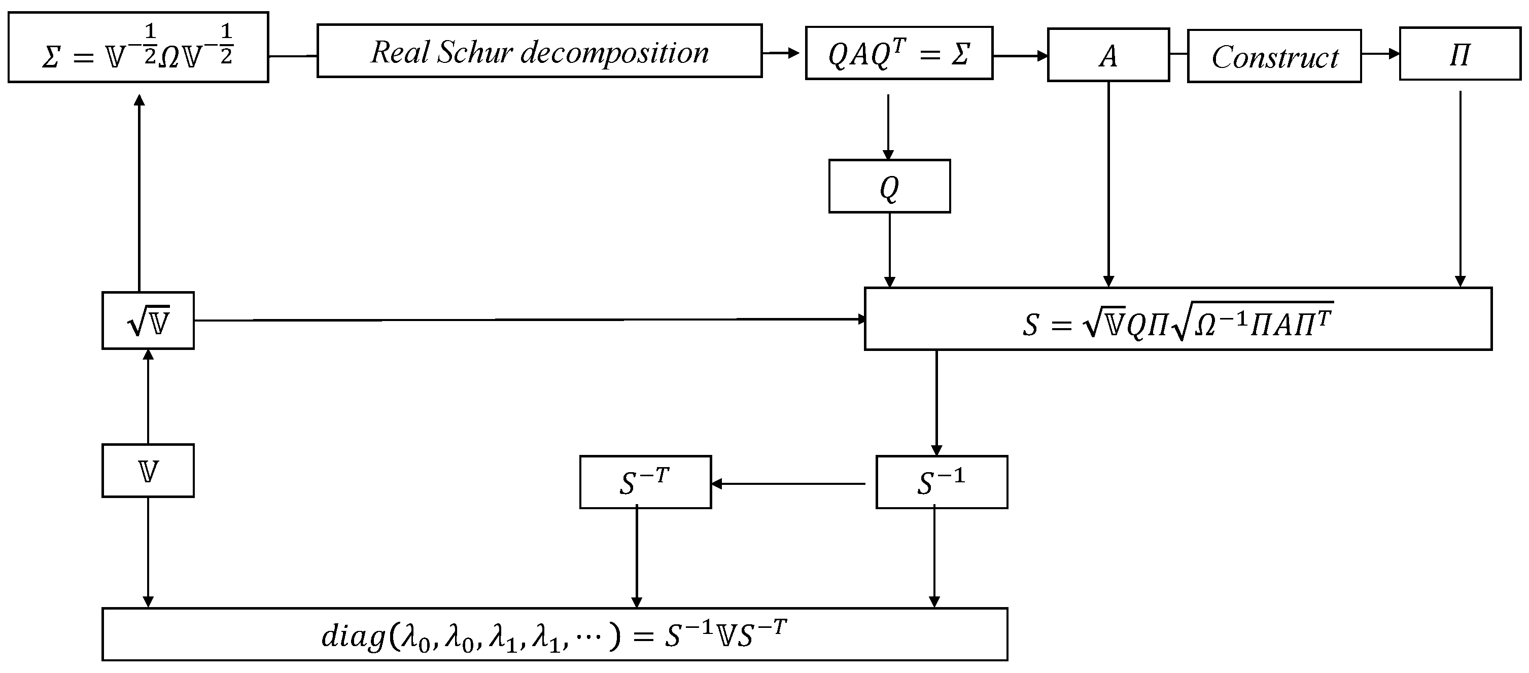
The specific computational steps are as follows:
- 1.
- Construct the matrix
- 2.
-
Using a real Schur decomposition, decompose the covariance matrix asThe matrix A will have a form similar to :Where are numerical values that may be positive or negative.
- 3.
-
Based on the specific structure of matrix A, construct a permutation matrix such that the signs and arrangement of the non-zero elements in A exactly match those in , i.e.The permutation matrix is a block-diagonal matrix, with each block being for positive and for negative .
- 4.
- The symplectic transformation matrix is given by:
- 5.
- Compute the Williamson decomposition
Appendix D. Details of the Rectangular Function Basis
Let the expression for the rectangular function be
Performing normalization such that , the normalization coefficient is found to be . Therefore, the normalized basis function is defined as:
The orthogonality is apparent. When , using the definition of the Riemann sum, the projection of a square-integrable function onto it is:
For the Dirac function, which does not belong to the square-integrable space , we must apply special treatment. Under the rectangular function basis, we proceed as follows: approximate as an extremely narrow rectangular pulse , where c We require that the resulting transformation correctly characterizes the evolution of each mode. From the previous analysis, X is a submatrix of a unitary matrix. Therefore, we require that
and is of approximately the same order of magnitude as I. Only then will it possess key properties similar to those of functions in . A specific calculation shows it is a scalar. Using the definition of the Riemann sum, it equals
where denotes the region of the image plane. Therefore, , so . Thus, .
References
- Tsang, M.; Nair, R.; Lu, X. Quantum Theory of Tuperresolution for Two Incoherent Optical Point Sources. Phys. Rev. X 2016, 6, 031033. [CrossRef]
- Napoli, C.; Piano, S.; Leach, R.; Adesso, G.; Tufarelli, T. Towards Superresolution Surface Metrology: Quantum Estimation of Angular and Axial Separations. Phys. Rev. Lett. 2019, 122, 140505. [CrossRef]
- Lupo, C.; Huang, Z.; Kok, P. Quantum Limits to Incoherent Imaging are Achieved by Linear Interferometry. Phys. Rev. Lett. 2020, 124, 080503. [CrossRef]
- Wang, B.; Xu, L.; Li, J.; Zhang, L. Quantum-Limited Localization and Resolution in Three Dimensions. Photonics Res. 2021, 9, 1522–1530. [CrossRef]
- Lupo, C.; Pirandola, S. Ultimate Precision Bound of Quantum and Subwavelength Imaging. Phys. Rev. Lett. 2016, 117, 190802. [CrossRef]
- Gessner, M.; Fabre, C.; Treps, N. Superresolution Limits from Measurement Crosstalk. Phys. Rev. Lett. 2020, 125, 100501. [CrossRef]
- Sorelli, G.; Gessner, M.; Walschaers, M.; Treps, N. Optimal Observables and Estimators for Practical Superresolution Imaging. Phys. Rev. Lett. 2021, 127, 123604. [CrossRef]
- Schnabel, R. Squeezed States of Light and Their Applications in Laser Interferometers. Phys. Rep. 2017, 684, 1–51. [CrossRef]
- Jia, W.; Xu, V.; Kuns, K.; Nakano, M.; Barsotti, L.; Evans, M.; Mavalvala, N.; LIGO Scientific Collaboration. Squeezing the Quantum Noise of a Gravitational-Wave Detector Below the Standard Quantum Limit. Science 2024, 385, 1318–1321. [CrossRef]
- Casacio, C. A.; Madsen, L. S.; Terrasson, A.; Waleed, M.; Barnscheidt, K.; Hage, B.; Taylor, M. A.; Bowen, W. P. Quantum-Enhanced Nonlinear Microscopy. Nature 2021, 596, E12. [CrossRef]
- Garces, G. T.; Chrzanowski, H. M.; Daryanoosh, S.; Thiel, V.; Marchant, A. L.; Patel, R. B.; Humphreys, P. C.; Datta, A.; Walmsley, I. A. Quantum-Enhanced Stimulated Emission Detection for Label-Free Microscopy. Appl. Phys. Lett. 2020, 117, 024002. [CrossRef]
- de Andrade, R. B.; Kerdoncuff, H.; Berg-Sorensen, K.; Gehring, T.; Lassen, M.; Andersen, U. L. Quantum-Enhanced Continuous-Wave Stimulated Raman Scattering Spectroscopy. Optica 2020, 7, 470–475. [CrossRef]
- Li, T.; Li, F.; Liu, X.; Yakovlev, V. V.; Agarwal, G. S. Quantum-Enhanced Stimulated Brillouin Scattering Spectroscopy and Imaging. Optica 2022, 9, 959–964. [CrossRef]
- Kolobov, M. I.; Fabre, C. Quantum Limits on Optical Resolution. Phys. Rev. Lett. 2000, 85, 3789–3792. [CrossRef]
- Sorelli, G.; Gessner, M.; Walschaers, M.; Treps, N. Quantum Limits for Resolving Gaussian Sources. Phys. Rev. Res. 2022, 4, L032022. [CrossRef]
- Brady, A. J.; Gong, Z.; Gorshkov, A. V.; Guha, S. Incoherent Imaging with Spatially Structured Quantum Probes. arXiv:2510.09521 [quant-ph] 2025. Available online: https://arxiv.org/abs/2510.09521 (accessed on 1 January 2026).
- Shapiro, J. H. The Quantum Theory of Optical Communications. IEEE J. Sel. Top. Quantum Electron. 2009, 15, 1547–1569. [CrossRef]
- Serafini, A. Quantum Continuous Variables: A Primer of Theoretical Methods, 2nd ed.; CRC Press: Boca Raton, FL, USA, 2023; pp. 38–39, 47, 77–83, 241–242.
- Nichols, R.; Liuzzo-Scorpo, P.; Knott, P. A.; Adesso, G. Multiparameter Gaussian Quantum Metrology. Phys. Rev. A 2018, 98, 012114. [CrossRef]
- Tan, S. Quantum State Discrimination with Bosonic Channels and Gaussian States. Ph.D. Thesis, Massachusetts Institute of Technology, Stanford, CA, USA, September 2010.
- Houde, M.; McCutcheon, W.; Quesada, N. Matrix Decompositions in Quantum Optics: Takagi/Autonne, Bloch-Messiah/Euler, Iwasawa, and Williamson. Can. J. Phys. 2024, 102, 497–507. [CrossRef]
- Bertero, M.; Boccacci, P.; Pike, E. R. Resolution in Diffraction-Limited Imaging, a Singular Value Analysis. Opt. Acta 1982, 29, 1599–1611. [CrossRef]
Figure 1.
The propagation process of the quantized optical field in a simple imaging system. The multimode optical field at the object plane, , together with the vacuum field , is projected onto . It then evolves through the imaging system, coupling with the vacuum field , to form the image plane optical field .
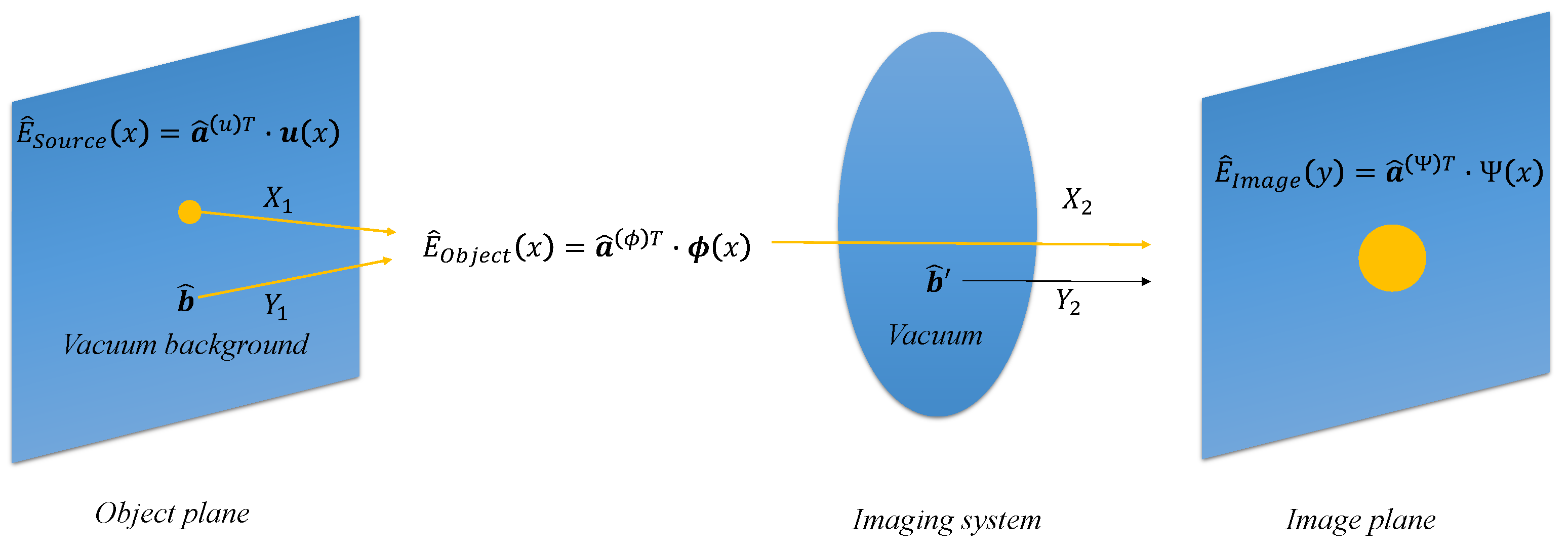
Figure 2.
Analysis of a simple imaging system. (Left) Optical path analysis. (Right) Calculation of the quantum Fisher information matrix (QFIM).
Figure 2.
Analysis of a simple imaging system. (Left) Optical path analysis. (Right) Calculation of the quantum Fisher information matrix (QFIM).
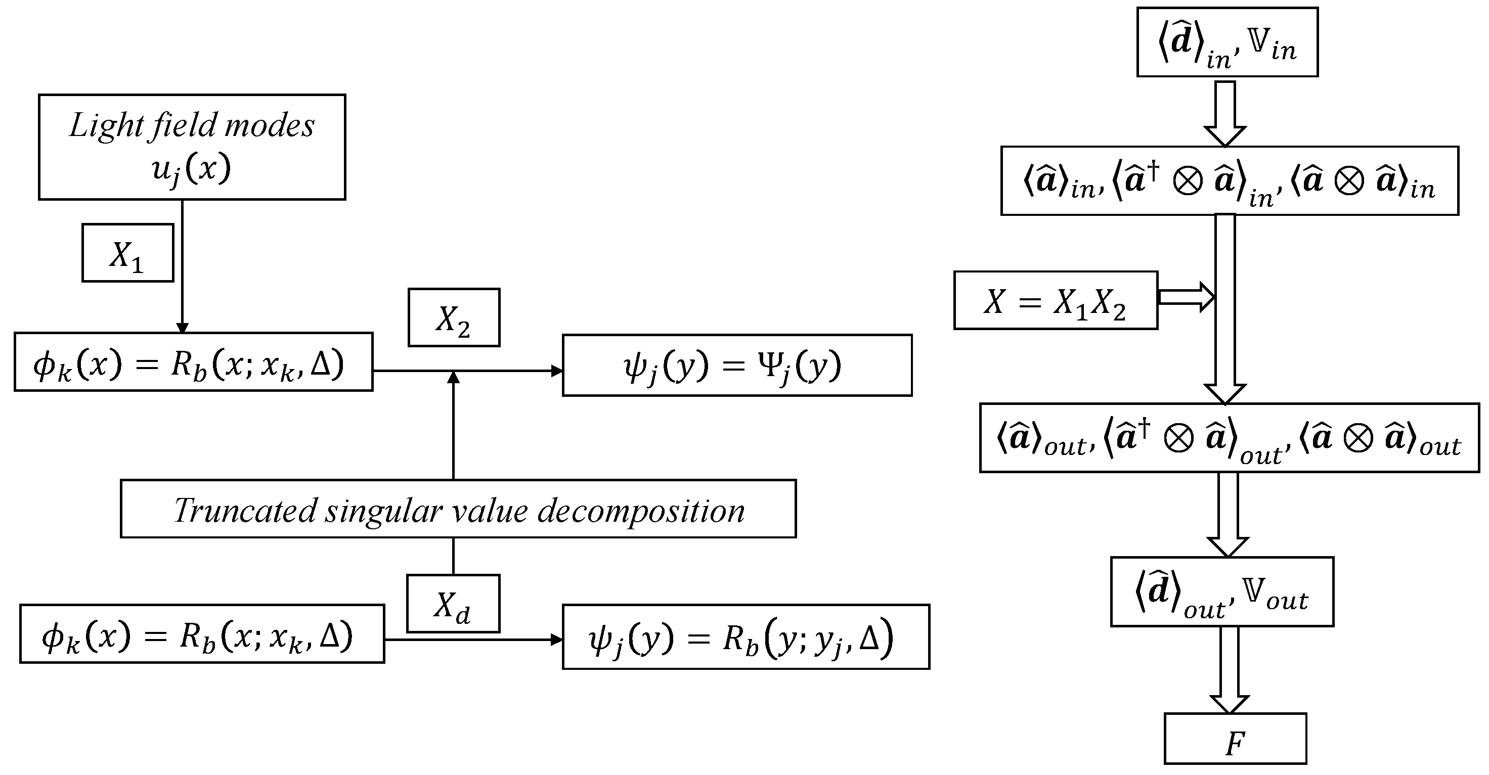
Figure 3.
Calculated results of the QFI. The upper panel shows the calculated values , and the lower panel presents the relative deviation from the method from reference.
Figure 3.
Calculated results of the QFI. The upper panel shows the calculated values , and the lower panel presents the relative deviation from the method from reference.
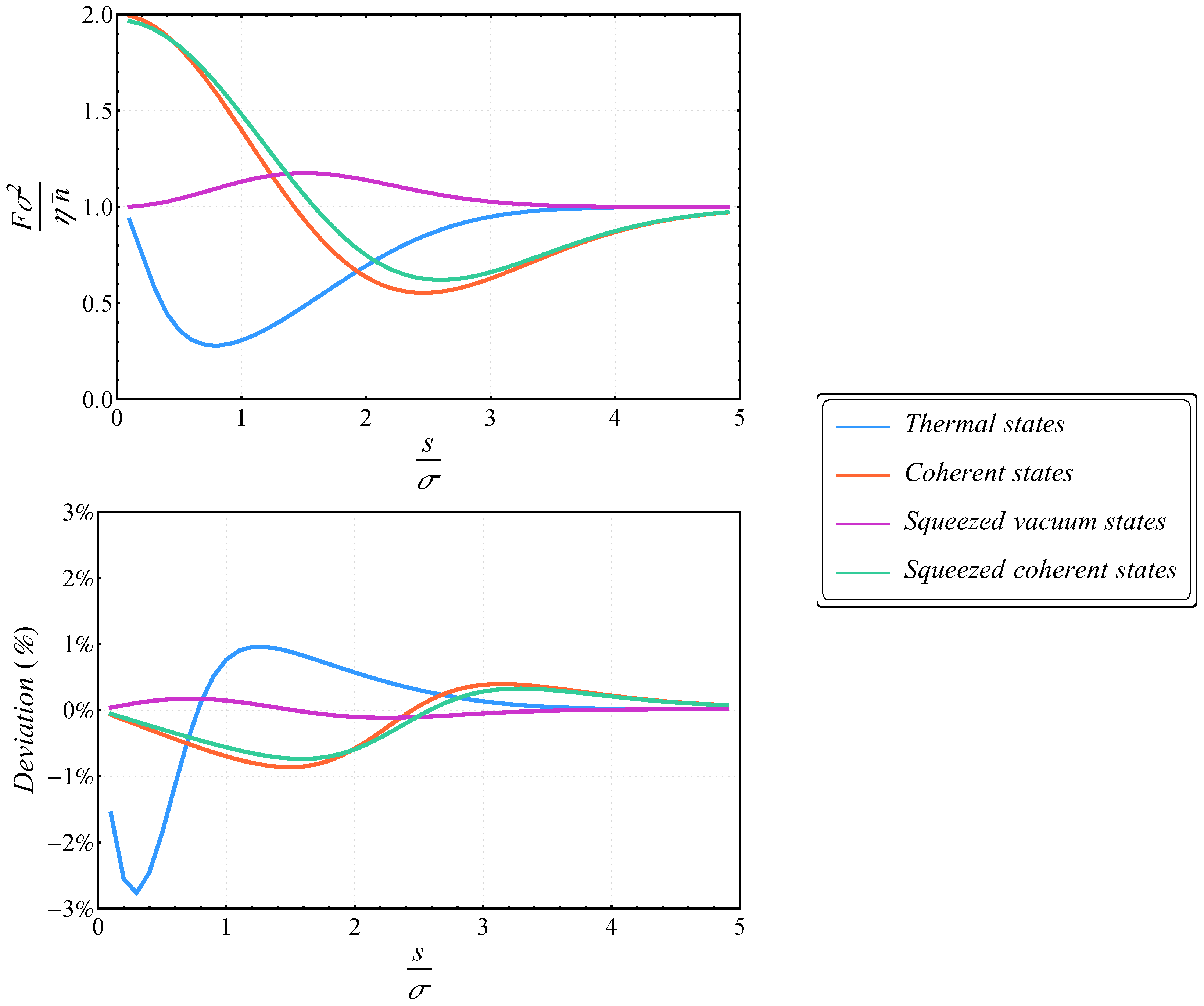
Figure 4.
(a) shows the complex amplitude distribution of the optical field . (c), (d), and (e) display the matrix elements of the QFIM corresponding to the parameter vector for expansions based on Hermite-Gaussian modes, Legendre polynomials, and right singular vector basis functions, respectively. (b) presents the values of the QCRB (for ) under different expansions, normalized relative to the result obtained from the right singular vector basis expansion, expressed as .
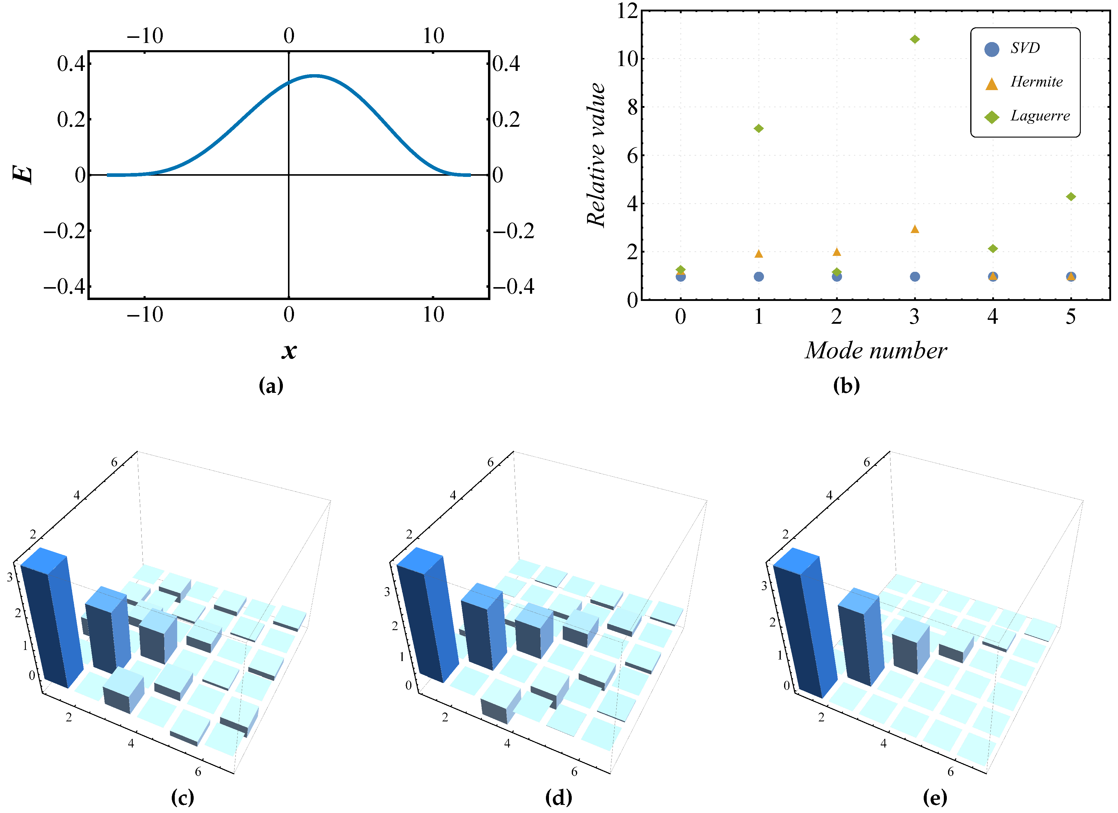
Figure 5.
The influence of increasing the mean photon number in the squeezed-part on the QCRB for estimating the parameter vector . The values shown are relative to the results for , expressed as . Here, (a) shows the complex amplitude distribution of the optical field obtained by reconstructing , and (b) shows the results when the parameter vector takes the specific value mentioned above. (c) displays the complex amplitude distribution of the optical field for , and (d) shows the corresponding results for this case.
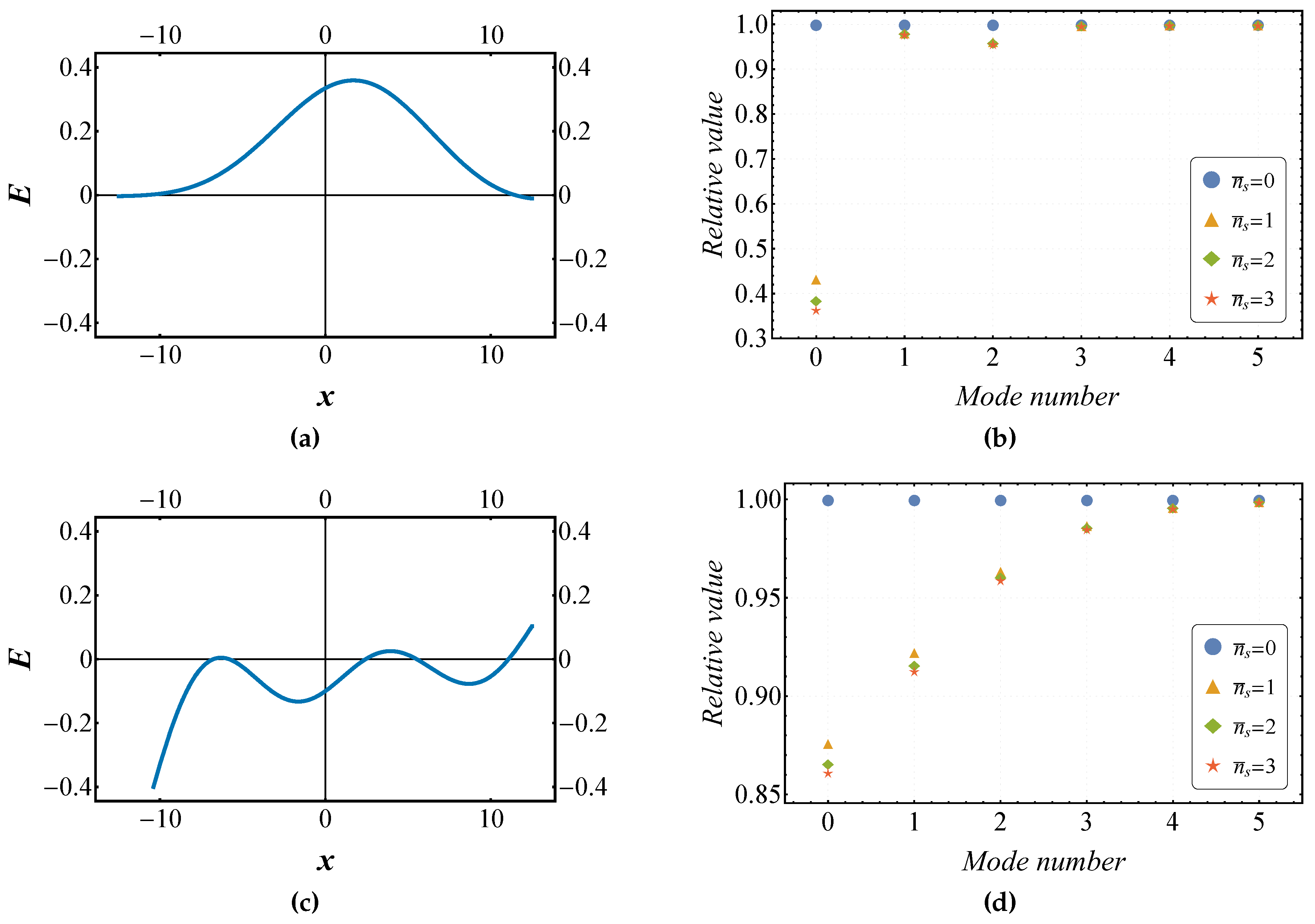
Figure 6.
QCRB for the parameter vector , which corresponds to the complex amplitude distribution shown in Figure 4 (a). The total mean photon number is , and the mean photon number from the squeezed part is . For clearer visualization, the coordinate axes are compressed via the transformation , while the tick labels indicate the original values.
Disclaimer/Publisher’s Note: The statements, opinions and data contained in all publications are solely those of the individual author(s) and contributor(s) and not of MDPI and/or the editor(s). MDPI and/or the editor(s) disclaim responsibility for any injury to people or property resulting from any ideas, methods, instructions or products referred to in the content. |
© 2026 by the authors. Licensee MDPI, Basel, Switzerland. This article is an open access article distributed under the terms and conditions of the Creative Commons Attribution (CC BY) license.
Copyright: This open access article is published under a Creative Commons CC BY 4.0 license, which permit the free download, distribution, and reuse, provided that the author and preprint are cited in any reuse.


