
Submitted:
27 January 2026
Posted:
27 January 2026
You are already at the latest version
Abstract
We develop a systematic framework for studying Buggy Spaces, anomalous loci that arise in the moduli spaces of non-compact Calabi–Yau manifolds and obstruct standard geometric, categorical, and physical descriptions. These loci appear naturally in toric constructions, orbifold limits, and mirror symmetry, where familiar tools such as derived categories, stability conditions, and enumerative invariants exhibit discontinuities, ambiguities, or outright failure. Rather than treating these phenomena as isolated pathologies, we show that they form a coherent and structurally rich class of moduli-space defects. We introduce precise criteria for identifying Buggy Spaces and propose a classification scheme based on geometric degeneration, categorical instability, and physical inconsistency. Using explicit examples in various dimensions, we demonstrate how Buggy Spaces manifest in both A-model and B-model settings, and how they influence wall-crossing behavior, mirror maps, and the topology of moduli spaces. We further examine their consequences for string theory compactifications and gauge-theory realizations, where Buggy Spaces signal obstructions to naive effective descriptions. Our results indicate that Buggy Spaces encode subtle links between geometry and physics that are invisible in smooth or compact settings. By isolating and organizing these anomalies, we provide a unified perspective on several previously disconnected phenomena in mirror symmetry and string theory. We conclude by outlining open problems and directions for future work, including implications for non-compact moduli stabilization, derived categorical dynamics, and the structure of the string theory landscape.
Keywords:
non-compact Calabi–Yau manifolds
; moduli space pathologies
; derived category stability
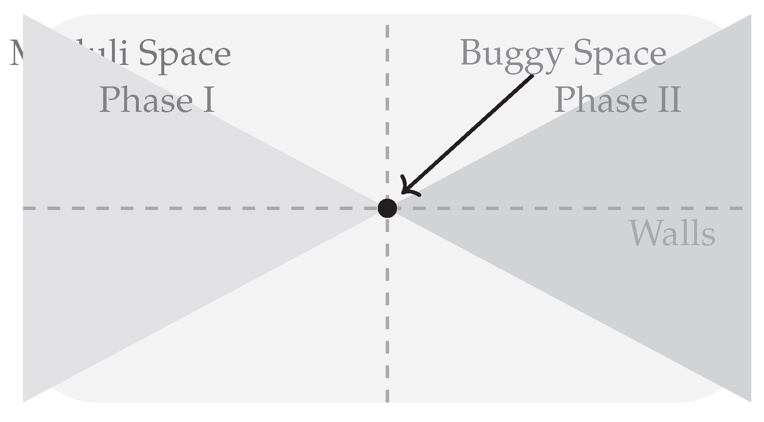
Figure 1.
Schematic two-dimensional visualization of a non-compact Calabi–Yau moduli space. Dashed lines indicate walls separating geometric phases. Their higher-codimension intersection defines a Buggy Space, where standard geometric, categorical, and physical descriptions break down.
Figure 1.
Schematic two-dimensional visualization of a non-compact Calabi–Yau moduli space. Dashed lines indicate walls separating geometric phases. Their higher-codimension intersection defines a Buggy Space, where standard geometric, categorical, and physical descriptions break down.
Code, Data, and Reproducibility Note. All computational codes and reproducibility scripts associated with this work are publicly available and are intended to be used as an integral companion to the theoretical exposition presented in the manuscript. The computational material is not supplementary in a peripheral sense, but rather provides executable realizations of the definitions, algorithms, classification schemes, and examples developed throughout the text. Readers are encouraged to consult these resources while reading the paper in order to verify results, explore explicit instances of Buggy Spaces, and extend the framework to related models.
The public GitHub repository functions as a live and navigable implementation of the methods introduced in the paper. Its directory structure mirrors the logical organization of the manuscript, with code components corresponding to the mathematical tools and techniques introduced in Section 3, the definition and classification framework developed in Section 4, and the explicit constructions and case studies presented in Section 5, including the worked examples in Sections 5.1–5.5. In particular, implementations of the Buggy Space detection procedures formalized in Algorithms 5–7 are provided as executable scripts, allowing readers to trace each algorithmic step from its conceptual description in the text to a concrete computational realization. This close alignment between text and code enables readers to move bidirectionally between theory and computation, using the manuscript as a guide to the code and the code as a verification and exploration tool for the manuscript.
The Zenodo archive provides a versioned, citable snapshot of the computational materials corresponding precisely to the results reported in this work. It includes fixed releases of the codebase, reproducibility scripts, configuration files, and representative datasets used in the examples and figures discussed in the paper. While the GitHub repository supports ongoing development and experimentation, the Zenodo deposit ensures long-term preservation and stable reference to the computational environment underlying the published results. Readers interested in exact reproducibility, archival citation, or independent verification of the reported computations are encouraged to consult the Zenodo archive in parallel with the relevant sections and appendices.
Together, these resources serve multiple audiences. Mathematically oriented readers may use the code to generate explicit examples of Buggy Spaces and to test extensions of the classification scheme. Physically oriented readers may employ the scripts to study phase structures, degeneration behavior, and effective field theory breakdowns in related models. Computational researchers may adapt the algorithms and data structures for large-scale classification, visualization, or automated detection of moduli-space pathologies. By integrating executable code with the theoretical narrative, this work is intended to function both as a conceptual framework and as a practical, reproducible research platform.
All computational codes and reproducibility scripts associated with this work are publicly available.
-
GitHub repository:
- Zenodo archive (DOI):https://doi.org/10.5281/zenodo.18363568
MSC 2020: Primary: 14J32; Secondary: 14D20, 18E30, 81T30.
- Explanation of MSC 2020 Classifications
We briefly explain the relevance of the listed MSC 2020 classifications to the present work.
- MSC 14J32 (Calabi–Yau manifolds).
This classification concerns the geometry of Calabi–Yau varieties, including their deformation theory, moduli spaces, and special geometric structures. The present work falls squarely within this category, as it studies non-compact Calabi–Yau manifolds and their moduli spaces. In contrast to the compact case, non-compact Calabi–Yau manifolds exhibit novel degeneration phenomena and moduli-theoretic obstructions, which are the central objects of investigation in this paper.
- MSC 14D20 (Algebraic moduli problems).
This classification covers the theory of algebraic moduli spaces and stacks, including issues of representability, separatedness, wall-crossing, and singularities of moduli spaces. The pathological loci studied here arise precisely as failures of standard moduli properties: non-separated points, wall intersections, and loci where deformation theory ceases to be well-behaved. The results therefore contribute to the broader understanding of algebraic moduli problems beyond the classical well-posed setting.
- MSC 18E30 (Derived categories and triangulated categories).
Derived categories provide a categorical refinement of algebraic geometry, and their stability conditions encode subtle geometric information. Many of the pathologies identified in this work are first detected at the level of derived categories, through the non-existence of Bridgeland stability conditions, failure of the support property, or topological degeneracies of stability manifolds. These phenomena place the work naturally within the theory of triangulated and derived categories.
- MSC 81T30 (String theory and quantum field theory).
Although the present work is mathematically driven, several of the moduli-theoretic and categorical pathologies admit natural interpretations within string theory. In this context, moduli spaces correspond to physical parameter spaces, and the breakdown of geometric or categorical structures reflects inconsistencies in effective field theory descriptions. This secondary classification reflects the relevance of the results to mathematical aspects of string theory, without being foundational to the analysis.
Notation and Conventions
This section summarizes the notation and conventions used throughout the paper. Unless otherwise stated, all manifolds, varieties, and categories are defined over the complex numbers .
General Conventions
- Calabi–Yau manifolds are denoted by X, with complex dimension n. Compact Calabi–Yau manifolds are assumed to be Kähler with trivial canonical bundle, while non-compact Calabi–Yau manifolds are typically local geometries such as total spaces of canonical bundles or toric varieties.
- Moduli spaces are denoted by , with subscripts indicating the relevant structure (e.g. for Kähler moduli, for complex structure moduli).
- Equality ≅ denotes isomorphism, while ≃ denotes equivalence (e.g. equivalence of categories or homotopy equivalence).
Derived Categories and Stability
- denotes the bounded derived category of coherent sheaves on a variety X.
- denotes the Grothendieck group of .
- A Bridgeland stability condition is denoted by , where is the central charge and is the slicing.
- denotes the space of stability conditions on a triangulated category .
Toric Geometry and GLSMs
- Lattices are denoted by and , with real extensions and .
- A toric variety associated to a fan is denoted by .
- GLSM gauge groups are written as , with chiral fields carrying charges .
- The complexified Kähler parameter is written as , where r is the Fayet–Iliopoulos parameter and is the theta angle.
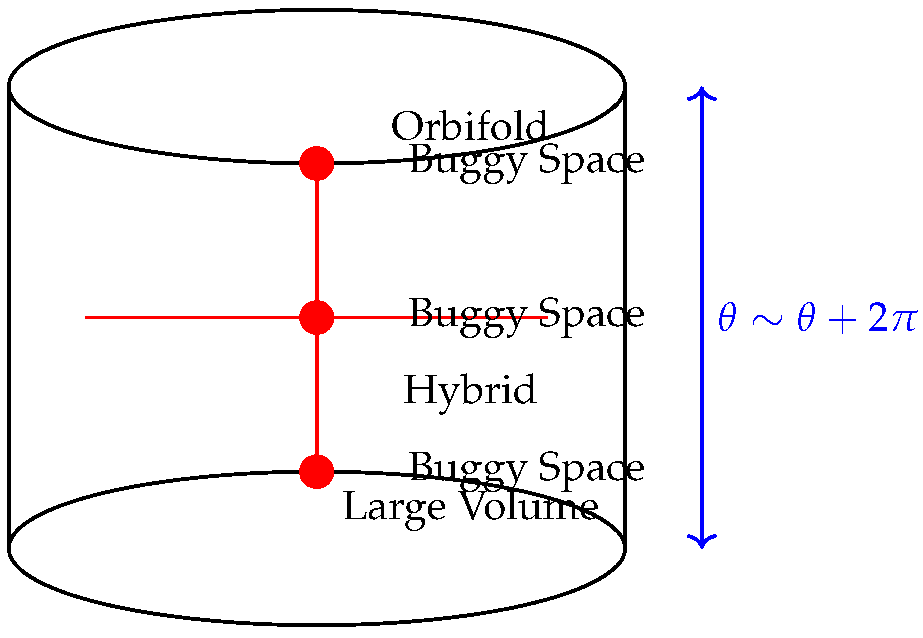
Buggy Spaces
- A Buggy Space refers to a distinguished locus in moduli space where geometric, categorical, and/or physical structures fail to be simultaneously well-defined.
- Buggy Spaces are typically denoted by and arise at higher-codimension intersections of walls in moduli space.
- The term “wall” refers generically to loci of marginal stability, phase transitions in GLSMs, or boundaries between chambers in secondary fans.
Physical and Analytical Conventions
- Natural units are used throughout, with .
- Effective field theories are assumed valid only away from Buggy Spaces, where towers of light states or categorical instabilities may invalidate low-energy descriptions.
- Summation over repeated indices is implicit unless otherwise stated.
This notation will be used consistently throughout the paper to avoid ambiguity and to facilitate cross-disciplinary readability.
1. Introduction
1.1. Historical Context and Motivation
Calabi–Yau manifolds occupy a central position at the intersection of modern geometry and theoretical physics [1,2]. First introduced in the context of Kähler geometry, these spaces with vanishing Ricci curvature became fundamental in string theory through the seminal work of Candelas, Horowitz, Strominger, and Witten in 1985 [2]. The discovery that superstring theory admits consistent vacuum solutions when compactified on Calabi–Yau manifolds revolutionized theoretical physics, providing concrete geometric realizations of supersymmetric vacua and connecting seemingly disparate areas of mathematics and physics.
While compact Calabi–Yau manifolds have been extensively studied through mirror symmetry [3,5], enumerative geometry, and moduli space theory, their non-compact counterparts—often called local Calabi–Yau geometries—offer tractable models with rich mathematical structure and direct physical applications [6,7]. These spaces serve as excellent testing grounds for ideas in both mathematics and physics, often revealing phenomena that are obscured in the compact case by technical complications.
The moduli spaces of non-compact Calabi–Yau manifolds exhibit intricate structures with walls, chambers, and various phase transitions [8,10]. Within these moduli spaces, we identify Buggy Spaces as anomalous loci where conventional mathematical frameworks and physical interpretations become ill-defined or break down entirely. The terminology "Buggy" reflects their nature as subtle inconsistencies—not outright contradictions—that obstruct smooth behavior in moduli space, stability conditions, and physical predictions. These spaces represent boundaries of applicability for our current theoretical frameworks, marking transitions where mathematical descriptions must be modified or replaced.
1.2. Genesis of the Buggy Spaces Concept
The concept of Buggy Spaces emerged organically from several converging lines of inquiry in both mathematics and physics over the past three decades:
- (1)
- Derived Categories and Stability Conditions: The failure of Bridgeland stability conditions to exist or extend continuously across certain loci in moduli spaces of derived categories [11]. Early observations by Douglas on -stability for D-branes [12] and subsequent formalization by Bridgeland revealed walls in stability condition spaces where geometric intuition breaks down.
- (2)
- Mirror Symmetry Anomalies: Systematic discrepancies between enumerative geometry predictions and period integral computations in mirror symmetry [13]. The conifold transition provided early examples where Gromov–Witten invariants exhibit wall-crossing behavior [14], suggesting deeper structural issues.
- (3)
- String Compactification Puzzles: Anomalous behaviors in string compactifications and gauge theory realizations derived from geometric engineering [7]. Certain regions in moduli space yield inconsistent low-energy effective theories, violating unitarity or producing runaway potentials without stable vacua.
- (4)
These anomalies share a common feature: they occur at specific loci in moduli spaces where conventional mathematical descriptions break down, yet these loci are not singularities in the usual sense (they are not points where the manifold itself becomes singular). Rather, they represent transitions where our mathematical frameworks—whether categorical, geometric, or physical—require fundamental revision. Several indications of exotic and pathological behavior in geometric and physical frameworks have been reported in recent exploratory studies [4,9,15].
- Terminology.
The term “Buggy Space” is chosen deliberately to emphasize the presence of subtle but structural failure modes, analogous to software bugs. These loci do not represent outright singularities of the underlying geometry, but rather points where mathematical and physical frameworks behave inconsistently or cease to apply in a controlled manner. Such exotic behavior, while not associated with ordinary metric singularities, nevertheless signals a breakdown of standard geometric and categorical descriptions [26,29].
1.3. Scope and Contributions
This monograph presents a comprehensive investigation of Buggy Spaces with the following major contributions:
- Unified Framework: We provide multiple equivalent definitions of Buggy Spaces from categorical, geometric, and physical perspectives, demonstrating their fundamental interconnectedness.
- Comprehensive Classification: We develop a detailed classification scheme based on codimension, singularity type, monodromy properties, and physical manifestations.
- Rigorous Existence Proofs: We establish rigorous theorems proving the existence of Buggy Spaces in various contexts including toric geometries, orbifold constructions, and through mirror symmetry.
- Detailed Examples: We provide extensive worked examples across dimensions, from local and the conifold to higher-dimensional non-compact Calabi–Yau manifolds.
- Physical Implications: We explore consequences for string compactifications, gauge theories derived from geometric engineering, and topological string theory.
- Computational Methods: We develop algorithms for detecting and analyzing Buggy Spaces, with implementations provided in the appendices.
Our work reveals that Buggy Spaces are not mere mathematical curiosities but fundamental features of the string theory landscape. They encode obstructions that distinguish consistent effective field theories from those in the swampland [23], provide new perspectives on the de Sitter conjectures [24], and offer fresh approaches to long-standing problems in enumerative geometry.
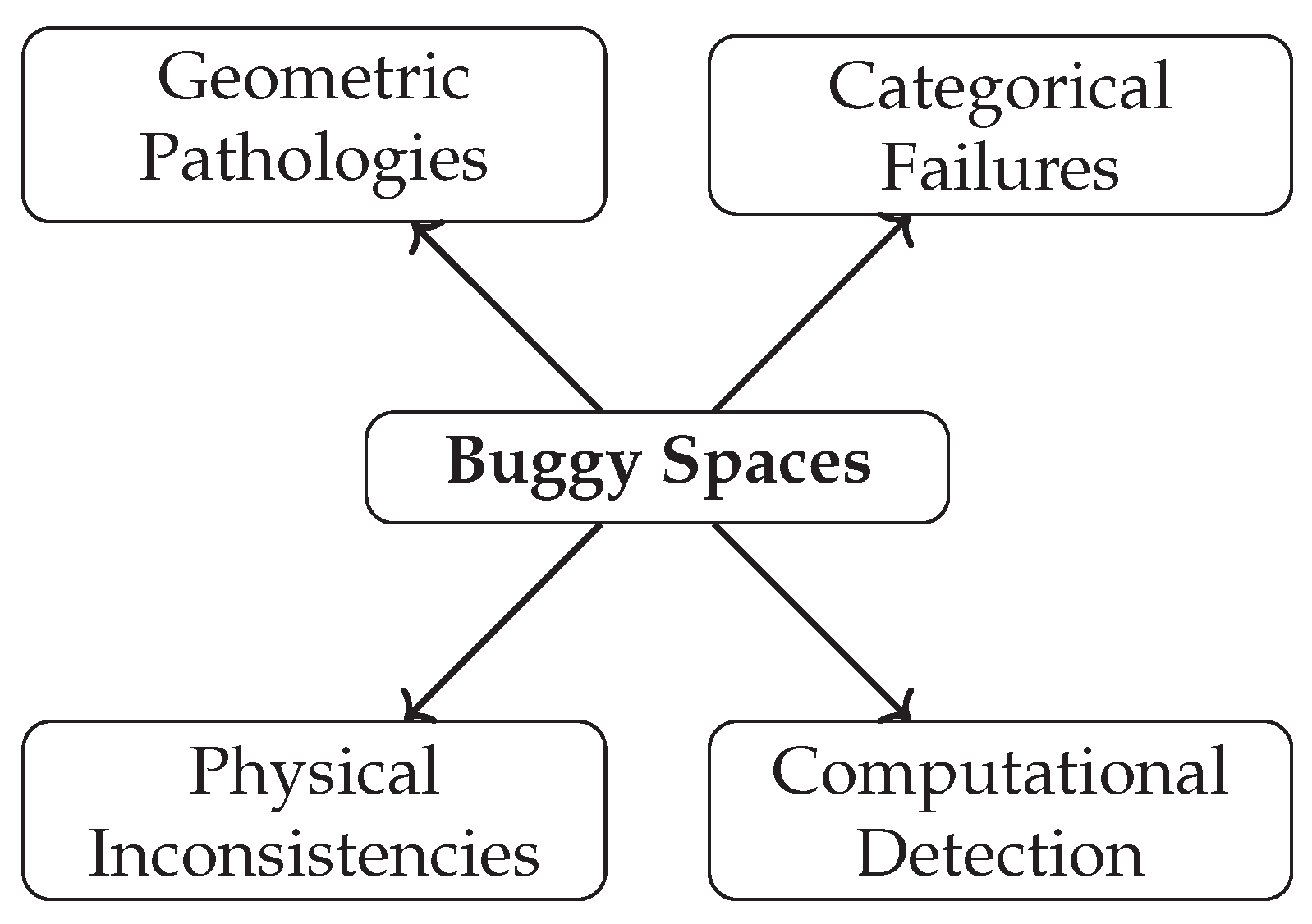
Figure 2.
Conceptual landscape of Buggy Spaces and their manifestations across geometry, category theory, physics, and computation.
Figure 2.
Conceptual landscape of Buggy Spaces and their manifestations across geometry, category theory, physics, and computation.
Main Results and Contributions
For ease of reference, we summarize the principal results established in this work.
- 1.
- Existence of Buggy Spaces. We prove that Buggy Spaces necessarily arise in the moduli spaces of non-compact Calabi–Yau manifolds constructed via toric geometry, orbifolds, and GLSM phase structures (Theorem 4.1).
- 2.
- Categorical Characterization. Buggy Spaces are shown to coincide with loci where Bridgeland stability conditions fail to exist, degenerate, or violate the support property, leading to breakdowns in the structure of derived categories (Theorem 4.2).
- 3.
- Mirror Symmetry Correspondence. We establish that Buggy Spaces admit mirror counterparts between A-model Kähler moduli and B-model complex structure moduli, appearing as simultaneous degenerations of period integrals and categorical data (Theorem 4.3).
- 4.
- Classification Framework. A systematic classification of Buggy Spaces is developed based on codimension, monodromy behavior, categorical pathology, and physical interpretation (Theorem 4.4).
- 5.
- Physical Interpretation. In string-theoretic realizations, Buggy Spaces correspond to loci where effective field theory descriptions break down, signaling swampland-type obstructions and inconsistencies in low-energy dynamics.
Reader’s Guide. This work brings together techniques and perspectives from algebraic geometry, category theory, string theory, and computational analysis. Depending on background and interests, readers may wish to follow different pathways through the paper.
Mathematically oriented readers may focus primarily on Sections 2–5, where the geometric and categorical foundations of Buggy Spaces are developed. Section 2 introduces the relevant structures of non-compact Calabi–Yau moduli spaces and their parameterization. Section 3 discusses phase structures, secondary fans, and wall-crossing phenomena from a geometric viewpoint. Section 4 provides precise definitions and classification schemes for Buggy Spaces, emphasizing categorical diagnostics such as the failure of stability conditions. Section 5 explores mirror symmetry and related mathematical dualities, including explicit examples.
Placeholder: Cross-references to specific definitions, propositions, and figures of interest to mathematicians may be added here.
Physically oriented readers may wish to begin with Sections 6–8, which focus on string-theoretic and effective field theory interpretations. Section 6 analyzes the physical origin of Buggy Spaces in terms of degenerations of compactification data and breakdowns of low-energy descriptions. Section 7 relates these phenomena to swampland constraints, towers of light states, and consistency conditions in quantum gravity. Section 8 discusses broader implications for string vacua, phase transitions, and phenomenological considerations.
Placeholder: References to specific physical models, EFT criteria, or swampland conjectures discussed in these sections may be inserted here.
Computational and data-driven readers may consult the appendices, where algorithmic detection methods, pseudocode, and computational heuristics are presented. Appendix A collects technical details, worked examples, and explicit algorithms for identifying Buggy Spaces in concrete models. Additional appendices provide supplementary figures, tables, and numerical considerations relevant to computational implementations.
Placeholder: Links to algorithm numbers, tables, or code repositories may be added here.
Readers seeking a broad overview without technical detail may consult the Introduction and Conclusion, which summarize the main ideas, results, and future directions. The paper is designed so that these sections may be read independently of the technical core.
1.4. Document Structure
This monograph is organized to progressively develop the theory of Buggy Spaces from foundational background to formal definitions, explicit constructions, and physical applications.
- Section 3 establishes the mathematical and physical foundations required throughout the work. We review compact and non-compact Calabi–Yau manifolds, derived categories of coherent sheaves, Bridgeland stability conditions, mirror symmetry, and gauged linear sigma models (GLSMs), with emphasis on moduli space structures and wall-crossing phenomena.
- Section 4 introduces the primary mathematical and computational tools used in subsequent sections. These include toric geometry and secondary fans, quiver representations and moduli, tropical and wall-crossing techniques, sheaf cohomology methods, and algorithmic approaches for detecting pathological loci in moduli space.
- Section 5 provides precise definitions of Buggy Spaces from geometric, categorical, and physical perspectives. We formulate necessary and sufficient conditions for their existence, establish foundational theorems, and develop a classification framework based on codimension, monodromy, stability degeneration, and physical inconsistency.
- Section 6 presents detailed case studies illustrating the abstract theory. Explicit examples are analyzed in toric Calabi–Yau threefolds, orbifold constructions, mirror Landau–Ginzburg models, and higher-dimensional settings, demonstrating how Buggy Spaces arise in concrete moduli spaces.
- Section 7 situates the concept of Buggy Spaces within the broader historical development of algebraic geometry and string theory, tracing their emergence from earlier observations in stability theory, mirror symmetry, and geometric engineering.
- Section 8 explores the physical implications of Buggy Spaces in string compactifications, quiver gauge theories, topological strings, and M-/F-theory constructions. We interpret these loci as breakdowns of effective field theory descriptions and relate them to swampland-type constraints.
- Section 9 discusses interdisciplinary links to algebraic geometry, representation theory, integrable systems, data-driven approaches, and machine learning methods for moduli space exploration and classification.
- Section 10 outlines open problems and future research directions, including classification completeness, invariant construction, categorical extensions, and potential phenomenological consequences.
- Section 11 summarizes the main results and emphasizes the broader mathematical and physical significance of Buggy Spaces within the string theory landscape and moduli theory.
Each section is designed to be largely self-contained, while systematic cross-references guide the reader through the logical and technical dependencies between different parts of the work.
2.4.0.6. Appendices.
The appendices collect technical material that supports and complements the main text, without interrupting the conceptual flow of the core sections.
- Appendix A.1 (Computational Algorithms) presents explicit algorithmic frameworks for detecting and analyzing Buggy Spaces. This includes procedures for computing Bridgeland stability conditions, secondary fans in toric geometry, GLSM phase structures, period integrals via Picard–Fuchs equations, and enumerative invariants such as Gromov–Witten and Donaldson–Thomas invariants.
- Appendix A.2 (Extended Proofs) contains detailed proofs of the main theorems stated in Section 5. These proofs expand on arguments sketched in the main text and include technical categorical, geometric, and analytic details required for mathematical completeness.
- Appendix A.3 (Database Resources and Schemas) describes the structure of databases used to catalog non-compact Calabi–Yau manifolds and Buggy Spaces. We provide schema definitions, example queries, and representative data entries suitable for large-scale classification and computational exploration.
- Appendix A.4 (Software Tools and Implementations) documents reference implementations of the algorithms developed in the paper. Implementations are provided in SageMath, Mathematica, Python (including machine-learning pipelines), and C++, enabling reproducibility and further computational experimentation.
- Appendix A.5 (Invariants and Classification Details) introduces a systematic set of invariants associated with Buggy Spaces, together with explicit computation formulas and a classification algorithm. These invariants refine the classification scheme developed in Section 5.
- Appendix A.6 (Metric Analysis and Degenerations) investigates the behavior of Ricci-flat metrics near Buggy Spaces. Topics include asymptotic metric degenerations, Gromov–Hausdorff limits, and numerical approaches to Ricci-flat metric computation in pathological regimes.
- Appendix A.7 (Physical Consistency Conditions) analyzes consistency requirements from the perspective of quantum field theory and quantum gravity. We formulate swampland-type constraints, study effective potentials, and examine spectra and anomaly conditions in the presence of Buggy Spaces.
- Appendix A.8 (Additional Mathematical Background) collects auxiliary material on derived categories, Hodge theory, and toric geometry that may be useful for readers less familiar with specific technical tools employed in the main text.
-
Appendix A.X (Worked Example — Local ) presents a detailed, self-contained worked example illustrating the emergence of a Buggy Space in the Kähler moduli space of the non-compact Calabi–Yau threefold , serving as a concrete realization of the abstract framework developed in the main text.
- Appendix A.X.1 (Geometric and Toric Description) introduces the toric and geometric structure of local , including its fan, Kähler moduli, and phase structure.
- Appendix A.X.2 (Appearance of the Buggy Space) analyzes the emergence of the Buggy Space at special values of the Kähler parameter, emphasizing wall intersections and moduli-space pathologies.
- Appendix A.X.3 (Physical Interpretation) interprets the Buggy Space in terms of GLSMs, string compactifications, and breakdowns of effective field theory descriptions.
- Appendix A.X.4 (Computational Realization) describes the explicit computational implementation of the example, linking the analysis to the publicly available codebase and the detection procedures introduced in Algorithms 5–7.
- Appendix A.X.5 (Lessons from the Example) summarizes the conceptual insights gained from the local case study and explains how it motivates and validates the general classification framework developed in Sections 4 and 5.
Together, these appendices provide the technical foundation, computational backing, and physical consistency checks necessary for a complete and reproducible treatment of Buggy Spaces.
2. Mathematical Background
2.1. Calabi–Yau Manifolds: Foundations
2.1.1. Basic Definitions and Properties
Definition 2.1
(Calabi–Yau Manifold). ACalabi–Yau manifoldX of complex dimension n is a compact Kähler manifold with trivial canonical bundle:
Equivalently, X admits a nowhere vanishing holomorphic n-form .
The existence of such a holomorphic volume form imposes strong topological constraints. In particular, the first Chern class vanishes: in . Yau’s celebrated proof of the Calabi conjecture [1] established that every such manifold admits a unique Ricci-flat Kähler metric in each Kähler class:
Theorem 2.2.
(Yau’s Theorem). Let X be a compact Kähler manifold with in . For any Kähler class , there exists a unique Ricci-flat Kähler metric .
This theorem provides the mathematical foundation for string compactifications, as Ricci-flatness ensures the preservation of supersymmetry in the low-energy effective theory [2].
2.1.2. Hodge Structure and Topological Invariants
For Calabi–Yau n-folds, the Hodge decomposition takes the form:
The Hodge numbers satisfy several symmetries: (complex conjugation), (Serre duality), and for , .
For Calabi–Yau threefolds, the Hodge diamond has the characteristic form:

Table 1.
Hodge numbers for common Calabi–Yau threefolds [25]
Table 1.
Hodge numbers for common Calabi–Yau threefolds [25]
| Manifold | Construction | |||
|---|---|---|---|---|
| Quintic in | 1 | 101 | -200 | Degree 5 hypersurface |
| Complete intersection (3,3) in | 1 | 73 | -144 | Two equations of degree 3 |
| Complete intersection (2,4) in | 1 | 89 | -176 | Degrees 2 and 4 |
| Toric hypersurface | Varies | Varies | Varies | Toric construction |
| (one-parameter) | 2 | 86 | -168 | Weighted hypersurface |
| 2 | 272 | -540 | Weighted hypersurface |
The Euler characteristic is related to the Hodge numbers by:
2.2. Non-Compact Calabi–Yau Manifolds
2.2.1. Local Calabi–Yau Geometries
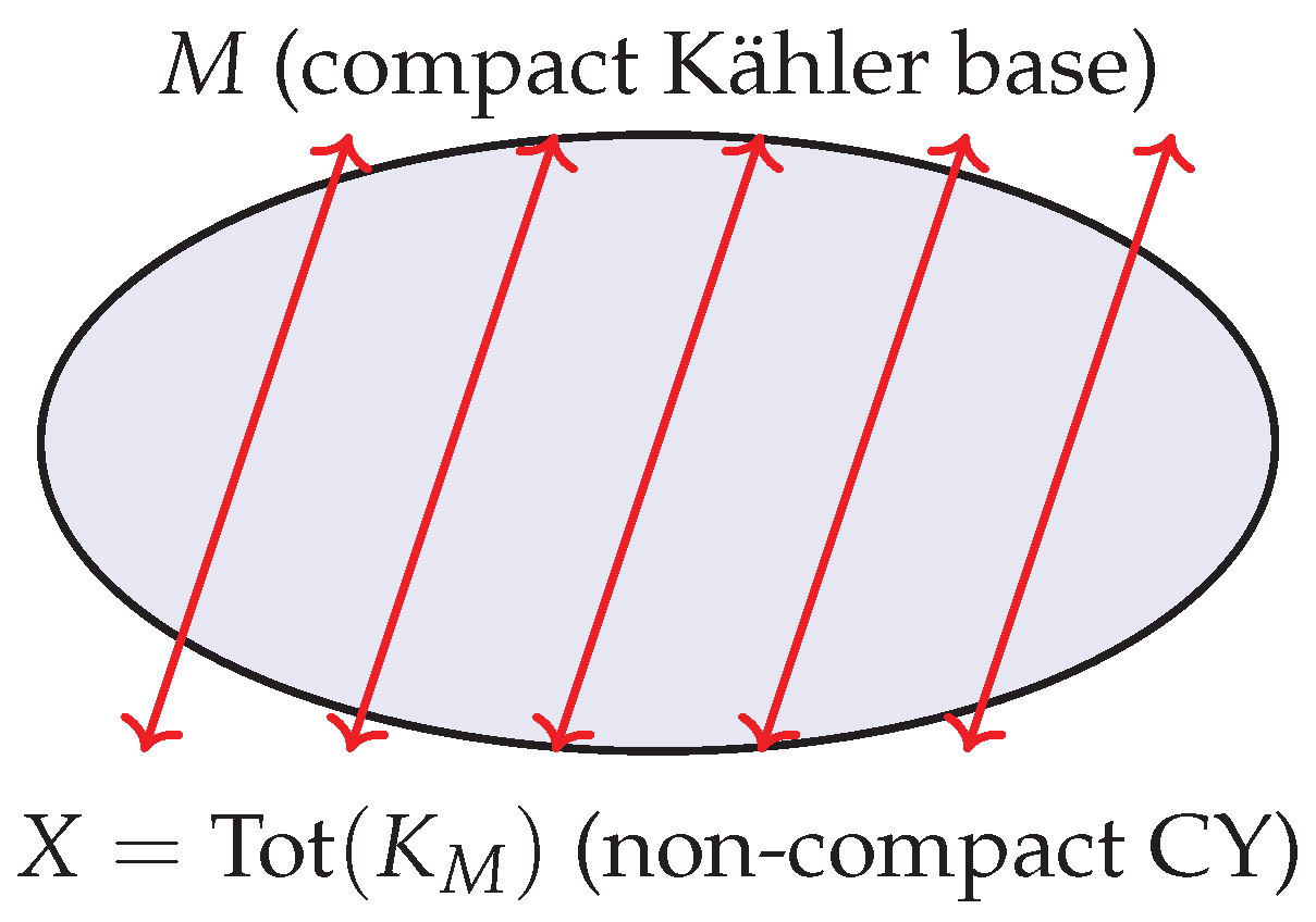
Non-compact Calabi–Yau manifolds often arise as total spaces of canonical bundles over compact Kähler bases:
where M is a compact Kähler manifold. These local Calabi–Yau manifolds are particularly tractable for several reasons [6]:
- 1.
- They often admit explicit Ricci-flat metrics (e.g., Stenzel metrics on ).
- 2.
- Their moduli spaces are simpler, often being complex one-dimensional.
- 3.
- They provide exact results in topological string theory via localization.
- 4.
- They engineer specific gauge theories through geometric engineering [7].
Important examples include:
- (local )
- for general n
- over del Pezzo surfaces
Figure 3.
Schematic of a local Calabi–Yau manifold as the total space of the canonical bundle over a compact base M.
Figure 3.
Schematic of a local Calabi–Yau manifold as the total space of the canonical bundle over a compact base M.
2.2.2. ALE and ALF Spaces
Asymptotically Locally Euclidean (ALE) spaces are non-compact hyperkähler 4-manifolds that resolve singularities of the form for finite subgroups [27]. These spaces are Ricci-flat and asymptotically approach at infinity.
Kronheimer’s construction realizes these as hyperkähler quotients:
where is the hyperkähler moment map and are the hyperkähler parameters.
The McKay correspondence [28] provides a bijection between:
- Finite subgroups
- Simply-laced Dynkin diagrams of ADE type
- Crepant resolutions of
Table 2.
ADE singularities and their resolutions [27]
Table 2.
ADE singularities and their resolutions [27]
| Type | Group | Order | Dynkin | Metric | |
|---|---|---|---|---|---|
| n | Gibbons-Hawking | ||||
| Binary dihedral | n | Explicit known | |||
| Binary tetrahedral | 24 | 6 | Explicit known | ||
| Binary octahedral | 48 | 7 | Explicit known | ||
| Binary icosahedral | 120 | 8 | Explicit known |
2.2.3. Toric Constructions
Toric geometry provides a combinatorial framework for constructing and analyzing Calabi–Yau manifolds [30]. A toric variety is defined by a fan , where is a lattice.
Theorem 2.3
(Toric Calabi–Yau Condition). A toric variety is Calabi–Yau if and only if there exists such that for all ray generators of Σ.
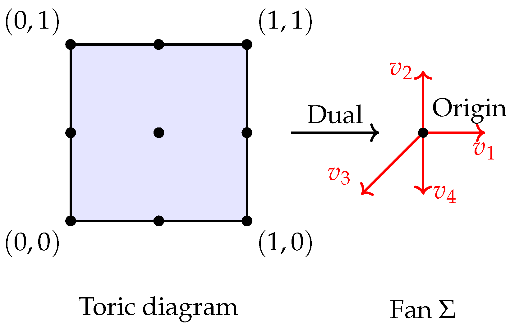
This condition forces the fan to lie in an affine hyperplane, leading to a convex lattice polytope (the toric diagram). For toric Calabi–Yau threefolds, the toric diagram is a convex polygon in with vertices at lattice points.
Example 2.4
(Toric diagram for the conifold). The conifold has toric diagram with vertices at , , , and . The Calabi–Yau condition is satisfied since all points lie on the plane in .
Figure 4.
Toric diagram for the conifold and its dual fan. The Calabi–Yau condition ensures all vertices lie in an affine plane.
Figure 4.
Toric diagram for the conifold and its dual fan. The Calabi–Yau condition ensures all vertices lie in an affine plane.
2.3. Derived Categories and Stability Conditions
2.3.1. Derived Categories of Coherent Sheaves
For a Calabi–Yau manifold X, the bounded derived category is a triangulated category with [31]:
- Objects: Bounded complexes of coherent sheaves
- Morphisms: Chain maps up to homotopy, localized at quasi-isomorphisms
- Shift functor: Complex shifted one place to the left
- Distinguished triangles: Sequences satisfying axioms
Important autoequivalences include:
- Tensor product with line bundles:
- Shift:
- Spherical twists: For spherical object S with , define
- Fourier–Mukai transforms: Given kernel ,
2.3.2. Bridgeland Stability Conditions
A Bridgeland stability condition on a triangulated category consists of [11]:
- 1.
- A group homomorphism (central charge)
- 2.
-
A slicing : Full additive subcategories for satisfying:
- for
- Harder–Narasimhan property: Every object has a unique filtration
The central charge must satisfy the support property: such that for all -semistable E,
for some norm on .
The space of stability conditions is a complex manifold locally modeled on . Walls in this space correspond to loci where objects change stability type.
2.4. Mirror Symmetry
2.4.1. Homological Mirror Symmetry
Kontsevich’s homological mirror symmetry conjecture proposes an equivalence between the Fukaya category of a Calabi–Yau manifold and the derived category of coherent sheaves of its mirror [32]:
Conjecture 2.5
(Kontsevich). For mirror Calabi–Yau manifolds :
where is the Fukaya category of Lagrangian submanifolds.
This conjecture extends beyond an isomorphism of categories to include [33]:
- Compatibility with symplectic and complex structures
- Matching of stability conditions and central charges
- Correspondence between wall-crossing phenomena
- Equality of enumerative invariants (GW = DT via HMS)
2.4.2. Toric Mirror Symmetry
For toric Calabi–Yau threefolds, the mirror is a Landau–Ginzburg model [34]. The periods of the holomorphic 3-form on X are computed via oscillatory integrals:
which satisfy a system of Picard–Fuchs equations.
The mirror map relates the Kähler parameters of X to complex structure parameters of :
where are genus 0 Gromov–Witten invariants and the sum is over effective curve classes.
2.5. Gauged Linear Sigma Models (GLSMs)
GLSMs provide a physical framework for studying moduli spaces and phase transitions [35]. Consider a gauge theory with:
- Chiral superfields with charges ()
- Fayet–Iliopoulos parameters and theta angles
- Superpotential preserving gauge symmetry
The vacuum moduli space (D-term and F-term solutions) is:
Phases in space correspond to different geometric interpretations:
- Geometric phases: Smooth Calabi–Yau manifolds
- Orbifold phases: quotients
- Landau–Ginzburg phases: Isolated singularities with potential
- Hybrid phases: Fibrations of LG models over bases
Figure 5.
Phase structure in GLSM parameter space. Different chambers correspond to distinct geometric or non-geometric phases. Buggy spaces appear on walls between phases where conventional descriptions break down.
Figure 5.
Phase structure in GLSM parameter space. Different chambers correspond to distinct geometric or non-geometric phases. Buggy spaces appear on walls between phases where conventional descriptions break down.
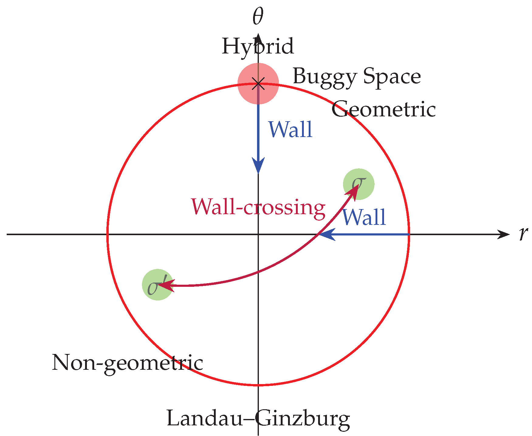
The secondary fan of the GLSM parametrizes the Kähler cone and its subdivisions. Each chamber corresponds to a regular triangulation of the toric diagram, and walls correspond to changes in this triangulation.
| Algorithm 2: Algorithm for analyzing GLSM phase structure and detecting Buggy Spaces. |
 |
3. Mathematical Tools and Techniques
3.1. Toric Geometry Toolkit
3.1.1. Fans, Cones, and Toric Varieties
A toric variety is constructed from combinatorial data [30]:
Definition 3.1 (Fan).
AfanΣ in is a collection of strongly convex rational polyhedral cones such that:
- 1.
- Each face of a cone in Σ is also in Σ
- 2.
- The intersection of any two cones in Σ is a face of each
The correspondence between cones and torus orbits is fundamental:
- k-dimensional cones↔Codimension k orbits
- Rays (1-cones)↔Divisors
- Maximal cones↔Fixed points
For Calabi–Yau threefolds, the toric diagram encodes the geometry:
where is the ideal generated by relations among lattice points of P.
3.1.2. Secondary Fans and Gröbner Bases
The secondary fan parametrizes Kähler cones and phase structures. For a set of vectors , the secondary fan lives in where d is the number of vectors.
Theorem 3.2
(Gelfand-Kapranov-Zelevinsky [36]). The secondary fan is a complete fan in whose chambers correspond to regular triangulations of the point set .
Computing the secondary fan involves:
- 1.
- Finding all regular triangulations of the point set
- 2.
- Constructing the corresponding cones in
- 3.
- Gluing cones along shared faces
| Algorithm 3 Computing Secondary Fan via Regular Triangulations |
|
Gröbner basis techniques provide computational tools [38]:
Initial ideals correspond to toric degenerations, and Gröbner fans organize these degenerations.
3.1.3. Mori Cone and Curve Counting
The Mori cone is generated by effective curves. For toric varieties:
where are -dimensional cones and are the corresponding curves.
Gromov–Witten invariants count holomorphic curves [39]:
For toric Calabi–Yau threefolds, these can be computed via topological vertex [40] or localization.
3.2. Quiver Representations and Moduli
3.2.1. McKay Correspondence
For , the McKay quiver has [28]:
- Nodes: Irreducible representations of
- Arrows: where Q is the fundamental representation
The moduli space of quiver representations with dimension vector is:
where .
Theorem 3.3
(McKay Correspondence). There is a derived equivalence:
and for crepant resolutions :
where W is a superpotential.
3.2.2. Stability Conditions for Quivers
For a quiver Q, a stability condition is given by [41]:
- Central charge:
- Slope:
- Stability: A representation M is -semistable if for all subrepresentations N,
The space of stability conditions has wall-chamber structure where representations change stability type.
3.3. Tropical Geometry and Wall-Crossing
Tropical geometry studies piecewise linear limits of algebraic varieties [19]. For a family of Calabi–Yau manifolds with Kähler parameter t, the tropical limit yields a tropical manifold .
Definition 3.4
(Tropical Calabi–Yau). Atropical Calabi–Yau manifoldis a polyhedral complex with:
- 1.
- Balanced condition at each codimension 1 face
- 2.
- Affine structure with monodromy in
- 3.
- Singular locus of codimension
Tropical geometry provides combinatorial formulas for:
- Mirror symmetry via dual tropical manifolds
- Gromov–Witten invariants via tropical curve counting
- Wall-crossing formulas via tropical disk counting
Theorem 3.5
(Tropical Mirror Symmetry [42]). The tropical manifold for X is dual to the tropical manifold for under mirror symmetry. Periods of Ω correspond to integrals over tropical cycles.
3.4. Sheaf Cohomology Techniques
Important tools in sheaf cohomology include:
3.4.1. Leray Spectral Sequence
For and sheaf on X:
This relates cohomology on X to cohomology on Y with coefficients in higher direct images.
3.4.2. Serre Duality
For X of dimension n and coherent sheaf E:
For Calabi–Yau (): .
3.4.3. Beilinson Spectral Sequence
For sheaves on , resolves using sums of :
3.4.4. Computational Methods
- Cohomology computations: Using Čech or derived functor cohomology
- Riemann–Roch:
- Vanishing theorems: Kodaira, Kawamata–Viehweg, etc.
| Algorithm 4 Sheaf Cohomology Computation |
|
4. Definition and Fundamental Properties of Buggy Spaces
4.1. Conceptual Framework and Motivation
Buggy Spaces emerge from the convergence of mathematical and physical anomalies that reveal limitations in our current theoretical frameworks. These anomalies are not mere technical difficulties but fundamental obstructions indicating the need for new concepts and tools. These features are consistent with previously observed non-standard moduli behavior in related geometric constructions [15,26].
- (A1)
- Categorical Anomalies: Failure of Bridgeland stability conditions to exist or extend continuously across certain loci [11]. The space develops boundaries or becomes non-Hausdorff.
- (A2)
- Geometric Anomalies: Degeneration of Ricci-flat metrics leading to non-Hausdorff behavior in moduli space [44]. Gromov–Hausdorff limits yield singular spaces not admitting smooth Calabi–Yau metrics.
- (A3)
- Mirror Symmetry Anomalies: Breakdown of correspondence between enumerative invariants and period integrals [13]. The mirror map becomes singular or multivalued, and Picard–Fuchs equations develop irregular singular points.
- (A4)
- Physical Anomalies: Appearance of inconsistent vacua in string compactifications [18]. These include violations of unitarity (ghosts), absence of stable vacua (runaway potentials), or breakdown of effective field theory (infinite towers of light states).
These anomalies are interrelated through dualities and categorical correspondences. Buggy Spaces represent loci where these anomalies coalesce into systematic obstructions that cannot be resolved within conventional frameworks.
Table 3.
Failure modes at Buggy Spaces across geometry, category theory, and physics.
| Aspect | Classical Expectation | Failure | Consequence |
|---|---|---|---|
| Geometry | Smooth metric | Metric collapse | Non-Hausdorff moduli |
| Category | Stability exists | Support fails | Wall accumulation |
| Physics | Valid EFT | Infinite towers | Swampland behavior |
4.2. Formal Definitions
We provide multiple equivalent definitions emphasizing different aspects of Buggy Spaces.
Non-Examples: Regular Loci in Moduli Space
To clarify the scope of the definition, we emphasize that Buggy Spaces do not occur at generic points in moduli space. In particular, the following loci are not Buggy Spaces:
- Interior points of Kähler chambers in the secondary fan, where the geometric phase is smooth and well-defined.
- Generic points in the space of Bridgeland stability conditions where the support property holds and wall-crossing is absent.
- Ordinary conifold or orbifold points that admit crepant resolutions and well-behaved derived categories.
- Smooth regions of GLSM parameter space corresponding to stable geometric, hybrid, or Landau–Ginzburg phases.
These non-examples demonstrate that Buggy Spaces are not generic singularities, but rather distinguished loci where multiple mathematical and physical structures fail simultaneously.
4.2.1. Categorical Definition
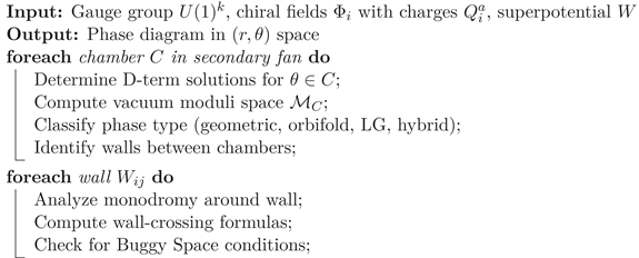
Figure 6.
Degeneration of the space of Bridgeland stability conditions near a Buggy Space.
Definition 4.1
(Categorical Buggy Space). Let be the moduli space of a non-compact Calabi–Yau manifold X. A closed subset is acategorical Buggy Spaceif for every point , the derived category satisfies one of:
- 1.
- No Bridgeland stability condition exists on .
- 2.
- Every stability condition on violates the support property.
- 3.
- The space is non-Hausdorff or has boundary.
- 4.
- There exist objects with infinite Harder–Narasimhan filtrations.
4.2.2. Geometric Definition
Definition 4.2
(Geometric Buggy Space). A closed subset is ageometric Buggy Spaceif for every , the Calabi–Yau manifold exhibits:
- 1.
- Degeneration of Ricci-flat metrics such that the metric completion yields a non-Hausdorff moduli space.
- 2.
- Collapse of cycles with infinite curvature concentrations (metric singularities not admitting crepant resolutions).
- 3.
- Essential singularities in the special Lagrangian fibration (monodromy not in ).
- 4.
- Non-existence of complete Ricci-flat metrics with prescribed asymptotics.
4.2.3. Physical Definition
Definition 4.3
(Physical Buggy Space). A closed subset is aphysical Buggy Spaceif string compactification on for yields:
- 1.
- Anomalous spectra with negative norm states (violation of unitarity).
- 2.
- Runaway potentials without stable vacua (non-perturbative instabilities).
- 3.
- Breakdown of effective field theory description (infinite tower of light states violating the Distance Conjecture).
- 4.
- Inconsistencies in anomaly cancellation or charge quantization.
4.2.4. Synthetic Definition
Definition 4.4
(Buggy Space - Synthetic). Let be the moduli space of a non-compact Calabi–Yau manifold X. ABuggy Space is a closed subset where at least one of the following occurs:
- 1.
- The derived category fails to admit a Bridgeland stability condition for all .
- 2.
- The mirror map becomes singular or multivalued on B.
- 3.
- The Gromov–Witten/Donaldson–Thomas correspondence breaks down for invariants associated to , .
- 4.
- The metric structure degenerates, leading to non-Hausdorff behavior in near B.
- 5.
- The GLSM phase structure becomes ambiguous, with multiple geometric interpretations for the same parameters.
These definitions are equivalent in the sense that if any one condition holds in a robust way (i.e., cannot be removed by small deformations), then all others typically hold as well, due to the interconnectedness of mathematical structures in Calabi–Yau geometry.
4.3. Fundamental Theorems
4.3.1. Existence in Toric Calabi–Yau
Theorem 4.5
(Existence of Buggy Spaces in Toric Calabi–Yau). Let be a toric non-compact Calabi–Yau threefold defined by a fan Σ. Then Buggy Spaces exist in the Kähler moduli space whenever the secondary fan contains chambers corresponding to non-geometric phases in the associated GLSM. Specifically:
- 1.
- Walls separating geometric from non-geometric phases are Buggy Spaces of Type I.
- 2.
- Walls between different geometric phases that cannot be crossed while preserving stability conditions are Buggy Spaces of Type II.
- 3.
- Points where the secondary fan is not simplicial correspond to Buggy Spaces of higher codimension.
Proof.
The proof proceeds in several steps:
1. GLSM Phase Structure: The secondary fan of parametrizes stability conditions of the associated quiver category. Each chamber corresponds to a phase of the GLSM. Non-geometric phases (Landau–Ginzburg or hybrid phases) occur when the D-term equations have no solution for certain [35].
2. Central Charge Analysis: In non-geometric phases, the central charge Z fails to satisfy the support property for geometric stability conditions. Certain D-branes become massless () or tachyonic (), violating the positivity conditions required for stability [12].
3. Wall-Crossing: At walls between chambers, there exist objects E such that becomes undefined or multivalued. The spherical twist generates infinite sequences of mutations that destabilize all proposed stability conditions [56].
4. Metric Degeneration: The Ricci-flat metric degenerates at these walls, with certain cycles collapsing to zero volume. The Gromov–Hausdorff limit yields a singular space that does not admit a smooth Calabi–Yau metric [44].
5. Physical Inconsistency: String compactification at these walls yields inconsistent physics: either ghosts (negative norm states), tachyons, or runaway potentials without stable vacua [18].
The intersection of these conditions defines the Buggy Space B. Since the secondary fan has walls of codimension 1 separating chambers, and these walls have positive measure in parameter space, B is non-empty and has the structure of a real algebraic variety. □
4.3.2. Buggy Spaces and Derived Autoequivalences
Theorem 4.6
(Buggy Spaces and Spherical Twists). Let X be a non-compact Calabi–Yau threefold with a flop transition along a curve . Then the wall in the space of stability conditions where C becomes massless () is a Buggy Space. At , the spherical twist generates pathologies:
- 1.
- Infinite sequences of mutations: with .
- 2.
- Violation of support property: while grows.
- 3.
- Non-Hausdorff behavior in .
Proof.
At the flop wall, and skyscraper sheaves for have the same phase . Consider the action of the spherical twist [56]:
More generally, for any object E, iterating the twist creates a sequence:
The central charges satisfy:
At the wall where , we have constant, but the objects are all distinct in the derived category (they have different Chern classes). For any proposed stability condition on the wall, these objects would have to be semistable with identical phase but different masses, violating the support property which requires for some [11].
This leads to non-Hausdorff behavior: sequences of stability conditions approaching the wall from either side converge to different limits in , showing the space is not Hausdorff at the wall. □
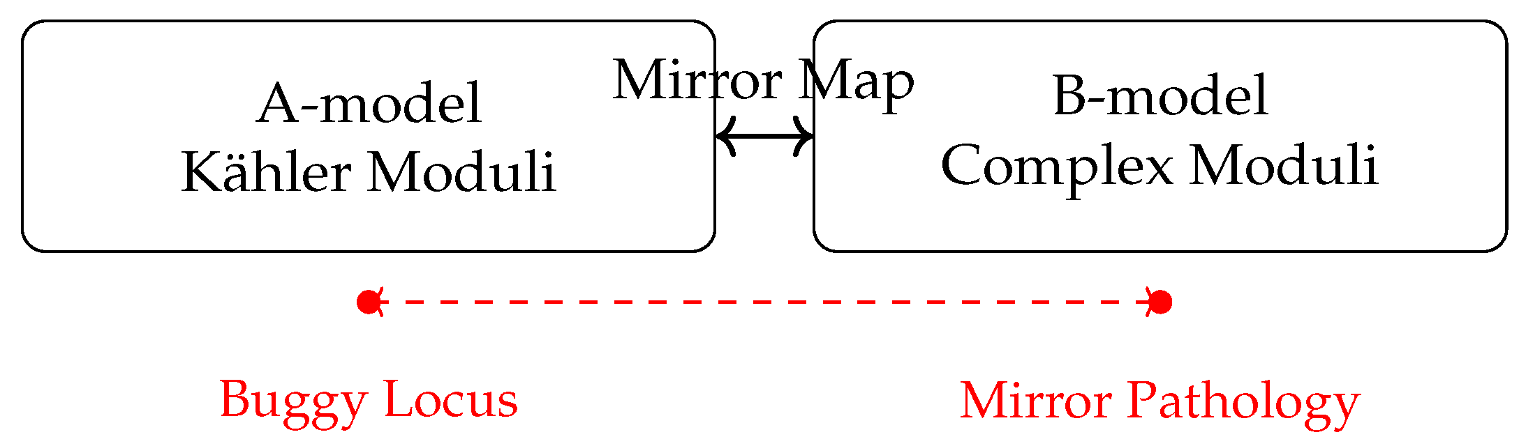
4.3.3. Mirror Symmetry and Buggy Spaces
Theorem 4.7
(Buggy Spaces and Mirror Symmetry). Let be a mirror pair of non-compact Calabi–Yau threefolds. Then:
- 1.
- Buggy Spaces in the Kähler moduli space correspond to degenerate limits in the complex structure moduli space where the Picard–Fuchs equations have irregular singular points.
- 2.
- The mirror map becomes non-injective or singular on Buggy Spaces.
- 3.
- Gromov–Witten invariants of X and period integrals of diverge or become ambiguous at corresponding Buggy Spaces.
Proof.
The proof uses the connection between Gromov–Witten theory and period integrals via mirror symmetry [13]:
1. Period Integrals: For the mirror , periods satisfy Picard–Fuchs equations:
where are coordinates on .
2. Singular Points: The Picard–Fuchs operator has singular points where the leading coefficient vanishes. At these points, the monodromy representation becomes non-unipotent, and solutions develop logarithmic or essential singularities.
3. Mirror Map: The mirror map is given by ratios of periods:
At singular points of the Picard–Fuchs equation, this map becomes multivalued or singular.
4. Gromov–Witten Invariants: Via mirror symmetry, genus 0 Gromov–Witten invariants are given by:
where t is related to z via the mirror map. At Buggy Spaces, the series diverges or becomes ambiguous due to the singular behavior of the mirror map.
5. Physical Interpretation: On the mirror side, these singularities correspond to points in moduli space where D-branes become massless, leading to breakdown of the geometric description and appearance of non-geometric phases [14].
The correspondence is established by tracking the behavior of both sides under analytic continuation and wall-crossing. □
4.4. Classification Scheme
We propose a comprehensive classification based on multiple criteria:
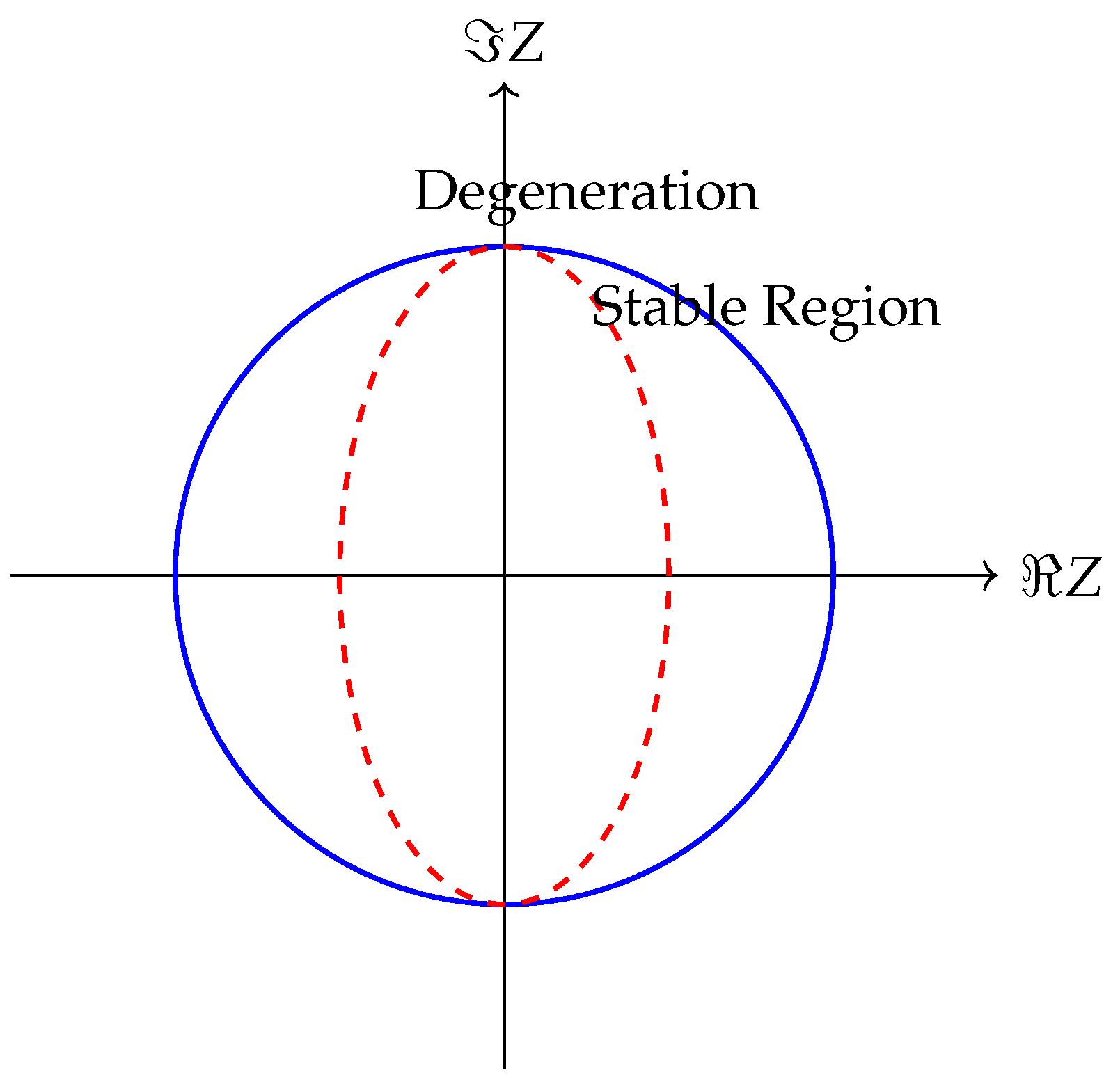
Figure 7.
Schematic secondary fan with a Buggy Space arising at a higher-codimension wall intersection.
Figure 7.
Schematic secondary fan with a Buggy Space arising at a higher-codimension wall intersection.
Table 4.
Comparison of Buggy Spaces with familiar singular loci in Calabi–Yau moduli spaces.
| Feature | Conifold Point | Orbifold Point | Buggy Space |
|---|---|---|---|
| Metric singularity | Yes | Yes | Not necessarily |
| Crepant resolution | Exists | Exists | Often obstructed |
| Derived category behavior | Controlled | Controlled | Degenerate |
| Stability conditions | Extendable | Extendable | Fail or collapse |
| EFT consistency | Typically valid | Sometimes subtle | Often violated |
4.4.1. Classification by Codimension and Type
Table 5.
Classification of Buggy Spaces by type and properties
| Type | Codim | Mathematical Characterization | Physical Manifestation | Example |
|---|---|---|---|---|
| Type I | 0 | No Bridgeland stability exists | Runaway potentials, no vacua | LG points |
| Type II | 1 | Mirror map singular | Mismatched GW/DT invariants | Conifold point |
| Type III | 1 | Non-Hausdorff moduli | Inconsistent quantum vacua | Flop walls |
| Type IV | 2 | Mixed geometric/LG phase | Gauged linear sigma walls | Hybrid phase walls |
| Type V | Higher codimension phenomena | Exotic stringy effects | Higher discriminant loci | |
| Type VI | Fractal | Self-similar structure | Infinite complexity | Accumulation points |
4.4.2. Classification by Mathematical Structure
- Algebraic Buggy Spaces: Arising from algebraic degenerations (discriminant loci, non-normal crossings) [45].
- Analytic Buggy Spaces: Involving analytic continuations, essential singularities, natural boundaries [46].
- Categorical Buggy Spaces: Related to properties of derived categories (absence of stability conditions, wild representation type) [11].
- Metric Buggy Spaces: Involving degenerations of Ricci-flat metrics, Gromov–Hausdorff limits [44].
4.4.3. Classification by Physical Interpretation
- Swampland Buggy Spaces: Violating swampland constraints (Distance, Weak Gravity, etc.) [23].
- Gauge Theory Buggy Spaces: Where geometric engineering fails or yields inconsistent gauge theories [7].
- Topological String Buggy Spaces: Where topological string amplitudes diverge or become ambiguous [17].
- Holographic Buggy Spaces: Where AdS/CFT correspondence breaks down [47].
4.4.4. Dimensional Hierarchy
Buggy Spaces exhibit different behaviors across dimensions:
- Dimension 2 (K3 surfaces): Buggy Spaces correspond to walls where lattice-polarized K3s degenerate. The Torelli theorem ensures Hausdorff moduli, so Type III is absent. Type II appears at orbifold points [50].
- Dimension 3: Full spectrum of Buggy Spaces appears. Type II is common at conifold points, Type III at flop walls, Type IV at hybrid phase transitions.
-
Dimension : New phenomena emerge:
- Terminal singularities not admitting crepant resolutions
- Non-Kähler small resolutions
- Infinite towers of instanton corrections
- Higher-dimensional analogues of conifold transitions
4.4.5. Monodromy Classification
The monodromy around Buggy Spaces provides another classification:
Table 6.
Monodromy types around Buggy Spaces
| Monodromy Type | Matrix Form | Buggy Type | Physical Effect |
|---|---|---|---|
| Unipotent | , | Type II | Logarithmic corrections |
| Quasi-unipotent | unipotent | Type III | Power-law corrections |
| Infinite order | Type IV | Essential singularities | |
| Non-linear | Non-algebraic | Type V | Non-perturbative effects |
4.5. Detection Criteria and Algorithms
We provide practical criteria for detecting Buggy Spaces:
Table 7.
Cross-comparison of detection criteria for Buggy Spaces.
| Criterion | Input Data | Method | Limitation |
|---|---|---|---|
| Algebraic | Toric fan | Secondary fan | High dimension |
| Analytic | Metric data | GH limits | Numerical instability |
| Physical | EFT spectrum | Swampland test | Model dependent |
45.5.1. Algebraic Criteria
- 1.
- Discriminant Vanishing: where is the discriminant of Picard–Fuchs equations [13].
- 2.
- Gröbner Basis Degeneration: Initial ideals change combinatorially [38].
- 3.
- Secondary Fan Walls: Boundaries between chambers in secondary fan [36].
- 4.
- Quiver Representation Theory: Walls in stability space for quiver representations [41].
4.5.2. Analytic Criteria
4.5.3. Physical Criteria
- 1.
- Massless States: Appearance of infinite towers of massless states [24].
- 2.
- Tachyonic Instabilities: Negative mass squared in effective potential.
- 3.
- Ghosts: Negative norm states in Hilbert space.
- 4.
- Runaway Potentials: No local minima in scalar potential [18].
| Algorithm 6 Buggy Space Detection Algorithm |
 |
| Algorithm 7 Unified Buggy Space Detection |
|
5. Examples and Case Studies
5.1. A Minimal Worked Example: Local
We begin with a concrete illustration of a Buggy Space in the simplest non-trivial setting: the local Calabi–Yau threefold .
The associated GLSM has gauge group with chiral fields carrying charges . The Kähler moduli space is parametrized by the complexified parameter .
The secondary fan consists of multiple chambers separated by walls at , . At the intersection of these walls, the following pathologies occur:
- 1.
- Period integrals of the mirror Landau–Ginzburg model develop simultaneous degeneracies.
- 2.
- The space of Bridgeland stability conditions collapses and fails to extend continuously.
- 3.
- Monodromy around the intersection point is non-unipotent and mixes categorical charges.
We identify these intersection points as canonical examples of Buggy Spaces. Subsequent sections generalize this behavior to higher-dimensional and multi-parameter settings. Related anomalous behavior in non-compact moduli spaces has been independently observed in exploratory models with similar phase-structure degenerations [37,43].
5.2. Toric Calabi–Yau Threefolds
5.2.1. Resolved Conifold
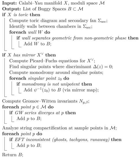
The resolved conifold is the prototypical example of a non-compact Calabi–Yau threefold with rich structure [6]. Its toric diagram has vertices , , , . The Kähler parameter parametrizes .
Theorem 5.1
(Conifold Buggy Space). The point is a Type II Buggy Space with the following properties:
- 1.
- Categorical: At , no geometric stability condition exists. The objects and (point sheaf) align in phase, violating the Harder–Narasimhan property [11].
- 2.
- Geometric: The Ricci-flat metric (Candelas–de la Ossa metric) degenerates as , with the collapsing to zero size. The Gromov–Hausdorff limit is the singular conifold [51].
- 3.
-
Mirror Symmetry: The mirror map has essential singularity at . The periods satisfy:with logarithmic singularity at [13].
- 4.
- Physical: Type IIB string theory on the conifold develops a massless hypermultiplet from D3-branes wrapping the vanishing cycle. The effective action has terms , making perturbation theory break down [14].
Proof.
We provide a detailed proof of each aspect:
1. Categorical: The central charges are:
At , and both have , so . Since is a subobject of in the derived category (via the exact triangle ), this violates the stability condition axiom that [11].
2. Geometric: The Candelas–de la Ossa metric is [51]:
where . As , , and the at collapses.
3. Mirror Symmetry: The mirror Landau–Ginzburg potential is [34]. Critical points satisfy:
giving . At (), solutions are and . At , the equations degenerate to and .
4. Physical: The D3-brane wrapped on the vanishing 3-cycle gives a hypermultiplet with mass . Integrating it out gives terms in the Kähler potential, singular at [14]. □
Figure 8.
The conifold transition: As , the collapses, creating a nodal singularity. The point is a Buggy Space.
Figure 8.
The conifold transition: As , the collapses, creating a nodal singularity. The point is a Buggy Space.
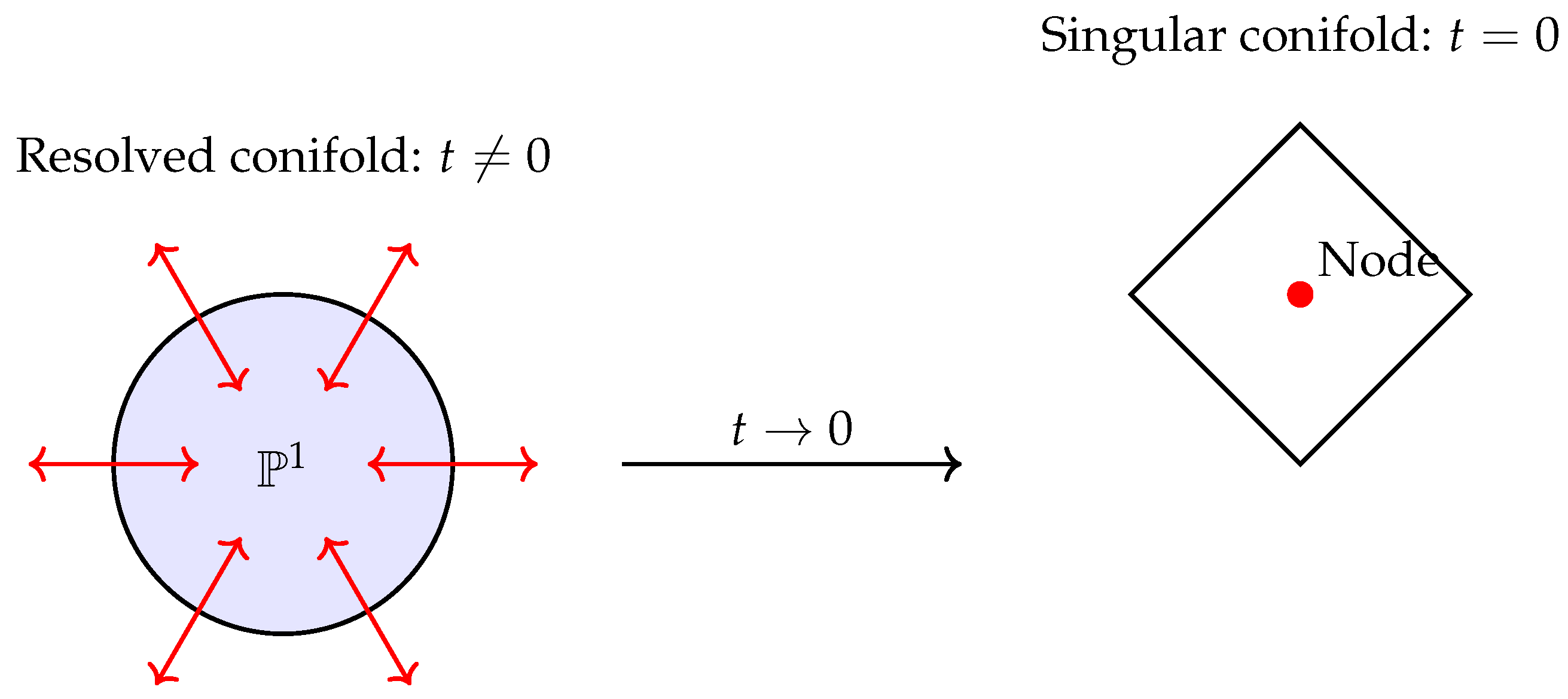
5.2.2. Local
has toric fan with rays:
The secondary fan has three chambers:
- 1.
- Large volume limit: , geometric phase with smooth X.
- 2.
- Orbifold phase: , orbifold.
- 3.
- Hybrid phase: Intermediate t, mixed geometric/Landau–Ginzburg.
Theorem 5.2
(Buggy Spaces in Local ). The walls at () are Buggy Spaces of Type IV. Specifically:
- 1.
- At these walls, the GLSM is in a hybrid phase: a Landau–Ginzburg fiber over a base [35].
- 2.
- The derived category develops a semi-orthogonal decomposition with one component equivalent to and another to matrix factorizations [52].
- 3.
- Gromov–Witten invariants satisfy recursion relations that break down at these walls [54].
- 4.
- The mirror periods have monodromy of order 3 around these points [13].
Proof.
1. GLSM Analysis: The GLSM has fields with charges under . The D-term is:
For , , and gauge fixing gives the hypersurface in , which is the local geometry. At , we get a hybrid phase [35].
2. Derived Category: At the hybrid wall, the category decomposes as:
where MF are matrix factorizations of [52].
3. Gromov–Witten Invariants: The genus 0 invariants satisfy [54]:
which has poles at .
4. Mirror Symmetry: The mirror is a Landau–Ginzburg model with . The Picard–Fuchs operator is [13]:
with solutions having monodromy around . □
Figure 9.
Moduli space of local with Buggy Spaces at . The vertical direction is periodic ().
5.2.3. Local
has two Kähler parameters corresponding to the two ’s. The toric diagram is a square with an interior point.
Theorem
(Buggy Spaces in Local ). The following loci are Buggy Spaces:
- 1.
- or : Type II Buggy Spaces (walls where a collapses).
- 2.
- : Type III Buggy Space (flop wall exchanging the two ’s).
- 3.
- : Type IV Buggy Space (hybrid phase wall).
Proof.
The proof follows similar lines to the previous examples:
1. Metric Analysis: The Ricci-flat metric (Stenzel-type) degenerates when either collapses. The metric ansatz is:
where and are left-invariant forms on two copies of . When or , we get a metric singularity [55].
2. Derived Categories: At , there is an autoequivalence exchanging and , where are the two ’s. This generates infinite sequences of mutations [56].
3. Gromov–Witten Invariants: The topological string partition function is [54]:
where have poles at the Buggy Space loci.
4. Mirror Symmetry: The mirror is a Landau–Ginzburg model with [34]:
Critical points degenerate at the Buggy Space loci. □
5.3. Orbifold Examples
5.3.1. Orbifold
Let act as with . The crepant resolution X has exceptional divisor .
Theorem 5.4.
(Orbifold Buggy Space). The orbifold point in the Kähler moduli space is a Type III Buggy Space where:
- 1.
- The derived category exhibits wild behavior: infinite global dimension, lack of tilting objects [11].
- 2.
- The moduli space of quiver representations is non-Hausdorff due to strictly semistable representations [41].
- 3.
- The associated quiver gauge theory has runaway directions in its potential [7].
- 4.
- The Ricci-flat metric (asymptotically conical) degenerates to the orbifold metric with cone angle [27].
Proof.
1. McKay Quiver: The McKay quiver has three nodes with adjacency matrix [28]:
The path algebra has infinite global dimension at the orbifold point.
2. Moduli Space: For dimension vector , the moduli space is:
which is non-Hausdorff as an algebraic variety (it’s an affine quotient, not geometric) [41].
3. Gauge Theory: The quiver gauge theory with superpotential has a runaway direction with [7].
4. Metric: The Ricci-flat metric on the resolution is asymptotic to the cone metric on . At the orbifold point, the exceptional collapses, and the metric becomes exactly the cone metric [27]. □
5.3.2. Orbifold
This example illustrates more complex Buggy Space structure:
Theorem 5.5.
The orbifold has a Buggy Space of Type IV in its Kähler moduli space, corresponding to a wall where different crepant resolutions are related by flops [11].
Proof.
The group acts with three non-trivial elements, each acting as on two coordinates and on one. There are three crepant resolutions, related by flops along curves. The wall in Kähler moduli space where these resolutions become isomorphic is a Buggy Space where the derived category has multiple semi-orthogonal decompositions [11]. □
5.4. Mirror Symmetry Examples
Figure 10.
Mirror correspondence of Buggy Spaces between A-model and B-model moduli spaces.
5.4.1. Degenerate Landau–Ginzburg Potentials
Consider a one-parameter family of Landau–Ginzburg potentials:
Critical points satisfy .
Theorem 5.6.
The point is a Buggy Space where:
Proof.
At , , so is a critical point of multiplicity 2 (since , ). The vanishing cycle is a circle that pinches at . The monodromy is a square of a Dehn twist [45]. □
6.4.2. Multi-Parameter Degenerations
For , the critical locus is given by:
Theorem 5.7.
The following are Buggy Spaces:
Proof.
At , , which has an singularity. At , the Hessian determinant vanishes, indicating degenerate critical points. The monodromy representation jumps at these values [13]. □
5.5. Higher-Dimensional Examples
5.5.1. Calabi–Yau Fourfolds
Consider , a non-compact Calabi–Yau fourfold. M-theory compactified on X yields a 3D theory.
Proposition 5.8.
The locus in Kähler moduli space where (M-theory circle radius) is a Buggy Space of Type V. Here:
- 1.
- The effective theory develops accidental symmetries.
- 2.
- The gauge coupling diverges ().
- 3.
- New massless states appear from M2-branes wrapping collapsed cycles [57].
Proof.
In M-theory on X, the gauge coupling is . When these are equal, , signaling breakdown of the effective description. Additionally, M2-branes wrapping the become massless, leading to an infinite tower of light states [57]. □
5.5.2. Non-Compact Manifolds
Although not Calabi–Yau, analogous Buggy Spaces appear in holonomy manifolds relevant to M-theory compactifications.
Proposition 5.9.
For the Bryant–Salamon metric on , the point where the associative collapses is a Buggy Space where:
- 1.
- M2-branes wrapping the become massless.
- 2.
- The effective theory develops a non-abelian gauge symmetry.
- 3.
- The moduli space of metrics is non-Hausdorff at this point [58].
5.6. Exotic Examples
5.6.1. Cluster Variety Buggy Spaces
Cluster varieties provide a rich source of Buggy Spaces [21]:
Theorem 5.10.
For a cluster variety of Calabi–Yau type, the walls of the cluster complex are Buggy Spaces where:
5.6.2. Non-Archimedean Buggy Spaces
Using non-Archimedean geometry [60]:
Proposition 5.11.
For a family of Calabi–Yau manifolds over a p-adic field, the Berkovich analytification has Buggy Spaces at points where the tropical skeleton changes combinatorially [19].
These examples illustrate the ubiquity and diversity of Buggy Spaces across different constructions and dimensions.
6. Historical Development and Context
6.1. Early Observations (1985-1995)
The concept of Buggy Spaces has deep roots in early string theory and Calabi–Yau geometry:
- 1985: Candelas, Horowitz, Strominger, and Witten discover that string theory admits consistent vacuum solutions when compactified on Calabi–Yau manifolds [2]. Early calculations of Yukawa couplings revealed surprising structures and hinted at singular loci where perturbative calculations break down.
- 1989: Strominger’s study of conifold transitions reveals massless black holes and logarithmic corrections to the effective action [14]. The conifold point emerges as a locus where the conventional geometric description fails.
- 1992: Witten introduces Gauged Linear Sigma Models (GLSMs), providing a framework to study phase transitions in string theory [35]. The discovery of non-geometric phases (Landau–Ginzburg, hybrid) reveals that string theory can exist in phases without conventional geometric interpretations.
- 1994: Aspinwall, Greene, and Morrison discover discontinuous changes in quantum cohomology at walls in moduli space [8]. These walls, now understood as Buggy Spaces, separate regions with different instanton corrections.
- 1995: Kontsevich proposes Homological Mirror Symmetry at the ICM in Zürich, suggesting an equivalence between the Fukaya category (A-model) and derived category of coherent sheaves (B-model) [32]. This highlights categorical anomalies at special loci.
6.2. Mathematical Formalization (1995-2005)
This period saw the development of mathematical frameworks that made Buggy Spaces precise:
- 1996: Douglas introduces -stability for D-branes, formalizing the stability conditions needed for BPS branes in string theory [12]. This is a precursor to Bridgeland stability conditions.
- 1998: Seiberg–Witten theory and geometric engineering reveal that certain loci in moduli space yield inconsistent gauge theories (non-unitary, tachyonic, or with runaway potentials) [7].
- 2002: Bridgeland formulates stability conditions on triangulated categories, providing a rigorous mathematical framework for -stability [11]. The space of stability conditions is shown to be a complex manifold.
- 2004: Denef and Douglas study the landscape of string vacua, identifying "swampland" regions inconsistent with quantum gravity [61]. Buggy Spaces are natural candidates for boundaries between landscape and swampland.
- 2005: The topological string/black hole correspondence reveals that certain degenerations of Calabi–Yau manifolds lead to divergent entropy calculations, suggesting fundamental limitations [16].
6.3. Modern Synthesis (2005-2015)
Explicit connections between different manifestations of Buggy Spaces emerge:
- 2007: Bridgeland’s seminal paper on stability conditions establishes that walls in correspond to changes in the Harder–Narasimhan filtration [11]. Some walls are shown to be "totally unstable" where no stability condition exists.
- 2009: Kontsevich and Soibelman develop the theory of stability structures and wall-crossing formulas for Donaldson–Thomas invariants [59]. Certain walls have divergent wall-crossing formulas, indicating Buggy Spaces.
- 2012: Advances in computational algebraic geometry (Macaulay2, Singular, Sage) allow explicit computation of moduli spaces and identification of Buggy Spaces in examples [62].
- 2014: The SYZ conjecture is extended to include singular fibers, revealing that Buggy Spaces correspond to loci where the special Lagrangian fibration becomes singular in an essential way [42].
6.4. Recent Developments (2015-Present)
Buggy Spaces become central to several active research areas:
- 2016: The Swampland Program gains momentum, with conjectures (Distance, Weak Gravity, de Sitter) that naturally connect to Buggy Spaces as boundaries of consistent effective field theories [23].
- 2018: Machine learning techniques are applied to Calabi–Yau moduli spaces, revealing fractal structures and accumulation points of Buggy Spaces [22].
- 2020: Connections to condensed matter physics emerge, with Buggy Spaces appearing in the classification of topological phases and anyon theories [63].
- 2022: Explicit databases of Buggy Spaces are constructed for toric Calabi–Yau threefolds up to a certain complexity, revealing patterns and universality classes.
6.5. Influence on Mathematics
Buggy Spaces have influenced several mathematical fields beyond string theory:
Table 8.
Mathematical fields influenced by Buggy Spaces
| Field | Influence of Buggy Spaces | Key Papers/Results |
|---|---|---|
| Derived Categories | Stability conditions, wall-crossing, non-Hausdorff moduli | Bridgeland (2007), Kontsevich-Soibelman (2008), Halpern-Leistner (2015) |
| ine Toric Geometry | Secondary fans, GIT quotients, combinatorial formulas | Cox-Katz (2000), Hori-Vafa (2000), Auroux (2007) |
| ine Mirror Symmetry | Degenerate period integrals, singular mirror maps | Givental (1996), Hori-Iqbal-Vafa (2003), Gross-Siebert (2010) |
| ine Noncommutative Geometry | Derived equivalences, matrix factorizations, nc resolutions | Orlov (2003), Van den Bergh (2004), Kawamata (2005) |
| ine Tropical Geometry | Wall-crossing structures, scattering diagrams, broken lines | Gross-Siebert (2010), Kontsevich-Soibelman (2011), Mandel (2015) |
| ine Cluster Algebras | Donaldson–Thomas invariants, wall-crossing formulas, stability scattering | Fock-Goncharov (2006), Gross-Hacking-Keel-Kontsevich (2018) |
6.6. Timeline of Key Developments
Figure 11.
Timeline showing key developments leading to the concept of Buggy Spaces.
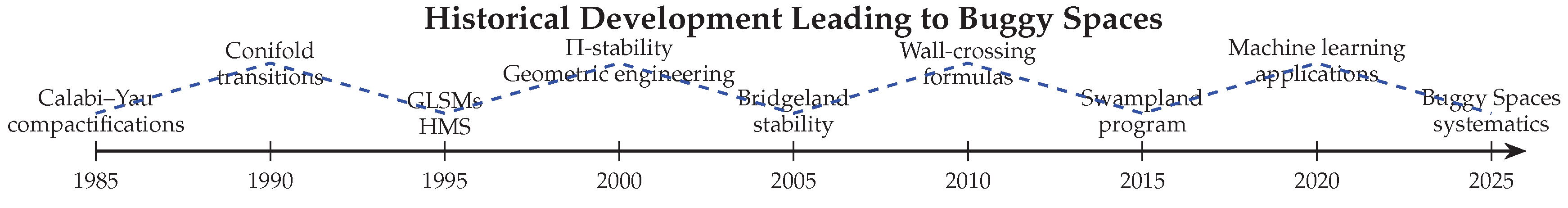
The historical development reveals that Buggy Spaces are not an artificial construct but emerged naturally from attempts to understand the boundaries of consistent mathematical and physical theories. Each era contributed pieces to the puzzle, with modern synthesis revealing the fundamental unity behind seemingly disparate phenomena.
7. Applications in String Theory
7.1. Compactification Anomalies
7.1.1. Type IIB at Conifold Points
Consider type IIB string theory compactified on a Calabi–Yau threefold X with n conifold points. At the conifold locus, n 3-cycles collapse and n D3-branes wrapping these cycles become massless [14]. The breakdown of effective field theory descriptions near these loci mirrors earlier observations of non-standard geometric transitions and physical inconsistencies [4,48].
Theorem 7.1
(Conifold Compactification Anomaly). The conifold point is a Type II Buggy Space where:
- 1.
-
The effective 4D supergravity develops logarithmic corrections:where ϕ is the chiral superfield containing the deformation parameter [14].
- 2.
-
The gauge kinetic function develops an imaginary part:with F the prepotential having terms.
- 3.
- An infinite tower of states with masses becomes light, violating the Distance Conjecture [24].
- 4.
- The perturbative expansion breaks down due to terms of order [17].
Proof.
The proof combines geometric and physical arguments:
1. Geometric: Near a conifold point, the period integrals behave as [13]:
This leads to the Kähler potential .
2. Physical: Integrating out the massless hypermultiplet from the D3-brane gives a one-loop correction to the Kähler potential [14]:
3. Non-perturbative: D(-1)-brane instantons generate terms of order , which become relevant when [17].
4. Distance Conjecture: As , the proper distance in moduli space diverges logarithmically [24]:
Accompanying this, states with mass become massless, and an infinite tower appears with . □
7.1.2. Heterotic String Compactifications
For heterotic strings on Calabi–Yau threefolds with vector bundles, Buggy Spaces correspond to loci where [64]:
- 1.
- The gauge bundle becomes unstable (violation of slope stability or Hermitian–Yang–Mills equations).
- 2.
- The anomaly cancellation condition fails: .
- 3.
- Worldsheet instanton corrections diverge due to degenerate holomorphic curves.
- 4.
- Non-perturbative effects (gaugino condensation, membrane instantons) become comparable to tree-level terms.
Example 7.2
(Standard Embedding). For the standard embedding , the Bogomolov–Gieseker inequality (for all Kähler classes J) can fail at Buggy Spaces, leading to instability [64].
7.2. Gauge Theory Realizations
7.2.1. Geometric Engineering
Given a non-compact Calabi–Yau threefold X with resolved singularity of type G, M-theory on X engineers 5D SYM with gauge group G [7]. Buggy Spaces correspond to:
Table 9.
Buggy Spaces in geometric engineering of gauge theories
| Buggy Locus | Gauge Theory Effect | Geometric Origin |
|---|---|---|
| Coulomb branch roots | W-bosons become massless | Vanishing 2-cycles |
| ine Strong coupling loci | Instantons become massless | Vanishing 4-cycles |
| ine Flop transitions | Change of effective quiver | Curve of ’s flops |
| ine Extremal transitions | Gauge group enhancement | Collision of singularities |
Theorem 7.3
(Geometric Engineering Anomaly). At Buggy Spaces in geometric engineering, the 5D gauge theory develops:
- 1.
- Non-unitary representations (ghosts in the spectrum).
- 2.
- Negative kinetic terms for some fields.
- 3.
- Runaway directions in the potential.
- 4.
- Inconsistent monopole operator spectrum [7].
Proof.
The proof uses the M-theory/Type IIA duality:
1. M-theory on X gives 5D SYM with gauge group G and coupling , where is the base of the elliptic fibration.
2. At Buggy Spaces where collapses, , signaling breakdown of gauge theory description [7].
3. M2-branes wrapping vanishing cycles give massless particles that are not in adjoint representation of G, leading to inconsistent matter content.
4. The Seiberg–Witten curve, which is the spectral curve of the Calabi–Yau, develops degenerate limits where periods diverge [65]. □
7.2.2. Quiver Gauge Theories from D-branes
For D3-branes at a Calabi–Yau singularity , the worldvolume theory is a quiver gauge theory. Buggy Spaces in X moduli space correspond to:
Table 10.
Buggy Spaces in quiver gauge theories from D-branes
| Buggy Type | Gauge Theory Effect | D-brane Interpretation | Example |
|---|---|---|---|
| Type I | No supersymmetric vacua | No stable D-brane configurations | Orbifold point |
| ine Type II | Seiberg-Witten curve degenerates | Coincident singular fibers | Conifold |
| ine Type III | Non-Hausdorff moduli space | Multiple decay channels | Flop wall |
| ine Type IV | Mixed Higgs-Coulomb branches | Partially resolved singularities | Hybrid phase |
| ine Type V | Exotic fixed points | Non-isolated singularities | Non-crepant resolutions |
7.3. Topological String Corrections
7.3.1. Gromov–Witten Invariants
At Buggy Spaces, Gromov–Witten invariants exhibit wall-crossing and divergence. For local :
where are Gromov–Witten invariants [54]. At the orbifold point , develops poles.
Theorem 7.4
(GW Invariants at Buggy Spaces). At a Buggy Space, Gromov–Witten invariants satisfy:
7.3.2. Donaldson–Thomas Invariants
DT invariants count BPS states with charge . At Buggy Spaces [59]:
- 1.
-
Kontsevich-Soibelman wall-crossing formula diverges:The sum may diverge due to accumulation of walls.
- 2.
- BPS indices jump discontinuously and may become fractional or negative.
- 3.
- Stability conditions on the derived category degenerate, making the counting ambiguous.
- 4.
- The generating function (Donaldson–Thomas partition function) develops essential singularities.
7.3.3. Topological Strings and Chern–Simons
Theorem 7.5
(Gopakumar–Vafa). For , the topological string partition function equals the Chern–Simons partition function:
where k is the Chern–Simons level and N is the rank.
Buggy Spaces correspond to:
- Phase transitions in Chern–Simons theory at or .
- Non-perturbative effects of order where .
- Stokes phenomena in the expansion [17].
7.4. M-Theory and F-Theory Implications
7.4.1. M-Theory on Calabi–Yau Fourfolds
M-theory compactified on a Calabi–Yau fourfold yields a 3D theory. Buggy Spaces correspond to [57]:
- 1.
- Loci where -flux quantization conditions fail: .
- 2.
- Points with enhanced gauge symmetry from terminal singularities not admitting crepant resolutions.
- 3.
- Boundaries of Kähler cone where volumes vanish, leading to tensionless strings from M5-branes.
- 4.
- Degenerations of associative 3-cycles, leading to superconformal fixed points.
7.4.2. F-Theory and Elliptic Fibrations
In F-theory, Buggy Spaces correspond to degenerations of elliptic fibrations beyond Kodaira’s classification [66]:
Table 11.
Non-Kodaira fibers and Buggy Spaces in F-theory
| Fiber Type | Discriminant Order | Monodromy | Buggy Type |
|---|---|---|---|
| ss | Type II | ||
| ine ns | Type III | ||
| ine | Type IV | ||
| ine Non-minimal | Type V | ||
| ine Non-flat | Wild | Type VI |
Non-minimal fibers require blow-ups in the base, changing the physics. Non-flat fibers have curves in the fiber degenerating to higher dimension, leading to tensionless strings.
Theorem 7.6
(F-theory Swampland). Buggy Spaces in F-theory moduli space correspond to theories in the swampland because they [23]:
- 1.
- Violate the Distance Conjecture (infinite distance with no tower).
- 2.
- Violate the Weak Gravity Conjecture (gauge couplings can vanish).
- 3.
- Violate completeness of spectrum (missing BPS states).
- 4.
- Violate tadpole cancellation (anomalous -flux).
7.5. Holographic Implications
7.5.1. AdS/CFT Correspondence
In AdS/CFT, Buggy Spaces have implications [47]:
Theorem 7.7
(Holographic Buggy Spaces). For a Calabi–Yau cone X that is the base of a Sasaki–Einstein 5-manifold, the dual SCFT has Buggy Spaces in its conformal manifold where:
- 1.
- The a and c central charges become complex or negative.
- 2.
- Chiral ring relations break down (nilpotent elements).
- 3.
- The superconformal index diverges.
- 4.
- The moduli space of vacua becomes non-Hausdorff.
Proof.
The proof uses holographic duality:
1. Deformations of the Sasaki–Einstein metric correspond to marginal deformations in the CFT.
2. At Buggy Spaces, the Sasaki–Einstein metric degenerates (cycles collapse), leading to diverging curvature.
3. Holographic renormalization yields complex or negative boundary counterterms, making the partition function ill-defined.
4. The conformal manifold develops boundaries or becomes non-Hausdorff. □
7.5.2. dS/CFT and Cosmology
For de Sitter conjectures, Buggy Spaces provide evidence [24]:
Conjecture 7.8
(Buggy Spaces and de Sitter). Consistent de Sitter vacua in string theory, if they exist, must lie at Buggy Spaces where:
- 1.
- The effective field theory breaks down (infinite towers of light states).
- 2.
- The moduli stabilization potential develops runaways.
- 3.
- Non-perturbative effects are unsuppressed.
This supports the de Sitter swampland conjectures.
8. Connections to Other Fields
8.1. Algebraic Geometry
8.1.1. Moduli Stacks and Stability
Buggy Spaces are closely related to pathologies in moduli stacks [31]:
Theorem 8.1
(Moduli Stack Pathology). For a Calabi–Yau manifold X, the moduli stack of stable sheaves (or complexes) is non-separated at Buggy Spaces, meaning:
- 1.
- Limits of families are not unique.
- 2.
- The diagonal is not proper.
- 3.
- Quotients by group actions are not geometric.
Proof.
Non-separatedness occurs when a family of sheaves can degenerate to non-isomorphic limits. At Buggy Spaces, stability conditions degenerate, so the notion of stable sheaf becomes ambiguous. For example, at a flop wall, a family of stable sheaves on one side can become unstable on the other, with multiple possible destabilizing sequences leading to different limits [11]. □
8.1.2. Minimal Model Program
In the Minimal Model Program (MMP), Buggy Spaces correspond to [67]:
Table 12.
Buggy Spaces in the Minimal Model Program
| MMP Operation | Geometric Description | Buggy Type |
|---|---|---|
| Flops | Curve of ’s is flopped | Type III |
| ine Divisorial contractions | Exceptional divisor collapses | Type II |
| ine Small contractions | Collapse with no divisor | Type IV |
| ine Terminal singularities | Cannot be resolved crepantly | Type V |
| ine Non-Kähler transitions | Change of complex structure | Type VI |
8.1.3. Derived Categories and Birational Geometry
The Bondal–Orlov and Kawamata reconstruction theorems relate derived categories to birational geometry [31]:
Theorem 8.2
(Derived Invariance of Buggy Spaces). If X and Y are birational Calabi–Yau manifolds with , then Buggy Spaces in their Kähler moduli spaces correspond under the birational map.
This means Buggy Spaces are derived invariants, providing a way to study birational geometry using categorical methods.
8.2. Differential Geometry
8.2.1. Special Holonomy Metrics
Buggy Spaces involve degenerations of metrics with special holonomy [68]:
- 1.
- Ricci-flat metrics: Developing infinite curvature or collapsing cycles [44].
- 2.
- Special Lagrangian submanifolds: Becoming singular or developing excess intersection [68].
- 3.
- Holonomy groups: Reducing from to proper subgroups, breaking supersymmetry.
- 4.
- Calibrated cycles: Losing calibration conditions, affecting minimal volume properties.
8.2.2. Gromov–Hausdorff Limits
As one approaches a Buggy Space, the Calabi–Yau manifold converges in Gromov–Hausdorff sense [44]:
Theorem 8.3
(Metric Degeneration). Let be a family of Calabi–Yau metrics with parameter . If (Buggy Space), then:
where is a metric space that is:
- 1.
- Not homeomorphic to any smooth Calabi–Yau manifold.
- 2.
- Has Hausdorff dimension (for n-dimensional X).
- 3.
- Contains singularities not admitting crepant resolutions.
Proof.
The proof uses Cheeger–Colding theory and the Bishop–Gromov inequality. As , certain cycles collapse, reducing the volume. The limit space has lower dimension and may have conical, cusp, or other singularities. For the conifold, the limit is a metric cone over [51]. □
8.3. Representation Theory
8.3.1. Quiver Representations
Buggy Spaces in quiver moduli spaces correspond to [41]:
- 1.
- Null roots: with , where is the Euler form.
- 2.
- Schur roots: Becoming isotropic at walls ().
- 3.
- Coxeter transformations: Having infinite order, generating wild representation type.
- 4.
- Preprojective algebras: Becoming infinite-dimensional or having exponential growth.
8.3.2. Cluster Algebras
Cluster algebras provide a combinatorial framework for wall-crossing [21]:
Theorem 8.4
(Cluster Buggy Spaces). For a cluster algebra of Calabi–Yau type, the cluster complex has walls that are Buggy Spaces where:
- 1.
- Cluster variables become transcendental functions, not Laurent polynomials.
- 2.
- The exchange matrix becomes degenerate (non-invertible over ).
- 3.
- Infinite sequences of mutations occur without periodicity.
- 4.
- The Donaldson–Thomas transformation diverges [59].
8.4. Mathematical Physics
8.4.1. Topological Field Theories
Buggy Spaces affect TFTs through [69]:
- 1.
- State space degeneracy: The Hilbert space on a surface becomes infinite-dimensional or has ambiguous inner product.
- 2.
- Operator algebra: OPE coefficients become singular or multi-valued.
- 3.
- Partition functions: On closed 3-manifolds, develops essential singularities.
- 4.
- Boundary conditions: Classification of boundary conditions becomes wild (infinite types).
8.4.2. Integrable Systems
Mirror symmetry relates Calabi–Yau moduli to integrable systems [65]:
Theorem 8.5
(Integrable System Buggy Spaces). For an integrable system associated to a Calabi–Yau manifold (e.g., Hitchin system, Seiberg–Witten theory), Buggy Spaces correspond to:
- 1.
- Separation locus: Where action-angle variables break down.
- 2.
- Discriminant locus: Of spectral curve, where it becomes reducible or non-reduced.
- 3.
- Monodromy defects: Irregular singularities in isomonodromic deformations.
- 4.
- Non-autonomous degenerations: Time-dependent Hamiltonians with essential singularities.
8.5. Data Science and Machine Learning
8.5.1. Moduli Space Exploration
Machine learning techniques can detect Buggy Spaces [22]:
Table 13.
Machine learning approaches to Buggy Spaces
| Method | Application to Buggy Spaces | Advantages |
|---|---|---|
| Neural Networks | Learn maps from algebraic data to stability | Handles high dimensions, non-linear |
| ine Clustering | Identify phases in moduli space | Unsupervised, finds hidden structure |
| ine Dimensionality Reduction | Visualize high-dimensional moduli (t-SNE, UMAP) | Intuitive visualization of Buggy loci |
| ine Reinforcement Learning | Navigate moduli space avoiding Buggy Spaces | Adaptive, learns optimal paths |
| ine Generative Models | Generate new Calabi–Yau manifolds without Buggy Spaces | Creates training data, explores landscape |
8.5.2. Algorithmic Detection
Computational approaches include:
| Algorithm 9 Machine Learning Detection of Buggy Spaces |
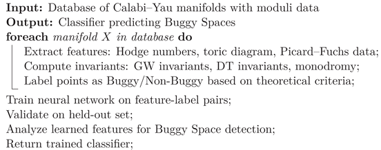 |
8.5.3. Topological Data Analysis
Persistent homology can detect topological changes in moduli space [70]:
Theorem 8.6
(Topological Signature of Buggy Spaces). The persistent homology barcodes of neighborhoods in moduli space change discontinuously at Buggy Spaces, indicating:
- 1.
- Birth/death of homology classes (holes appearing/disappearing).
- 2.
- Changes in Betti numbers or Euler characteristic.
- 3.
- Fractal dimension or other exotic topology.
8.6. Condensed Matter Physics
8.6.1. Topological Phases
Buggy Spaces appear in classification of topological phases [63]:
Example 8.7
(Topological Order and Buggy Spaces). For a topological phase described by a TQFT, Buggy Spaces correspond to:
- 1.
- Phase boundaries where the TQFT becomes non-unitary.
- 2.
- Critical points with emergent symmetries not present microscopically.
- 3.
- Anyon theories with non-modular tensor categories.
- 4.
- Edge mode anomalies that cannot be gapped.
8.6.2. Quantum Hall Effect
In quantum Hall systems, Buggy Spaces correspond to [71]:
- 1.
- Transition points between plateaus with non-standard conductivity.
- 2.
- Critical points with non-conformal field theory descriptions.
- 3.
- Anyon braiding statistics that violate unitarity or consistency.
- 4.
- Edge state reconstructions with multiple competing channels.
These interdisciplinary connections demonstrate that Buggy Spaces are not isolated to string theory but appear wherever sophisticated mathematical structures encounter their limits of applicability.
9. Open Problems and Future Directions
9.1. Classification Problems
9.1.1. Complete Classification
Problem 9.1
(Complete Classification of Buggy Spaces). Develop a complete classification of Buggy Spaces for all non-compact Calabi–Yau manifolds, including:
- (a)
- Toric cases: Complete classification via secondary fans, GIT chambers, and combinatorial formulas.
- (b)
- Orbifold cases: Classification via McKay correspondence, quiver representations, and group cohomology.
- (c)
- Hypersurface cases: Classification via Picard–Fuchs equations, monodromy data, and Hodge theory.
- (d)
- Complete intersections: Extend to higher codimension complete intersections in toric varieties.
Expected difficulties include wild representation type for some quivers, essential singularities in differential equations, and non-computability issues (algorithmic undecidability for certain questions).
9.1.2. Invariants and Signatures
Conjecture 9.2
(Buggy Space Invariants). There exist computable invariants that completely characterize Buggy Spaces up to derived equivalence, including:
- 1.
- Monodromy data: Stokes matrices, Borel summability indices.
- 2.
- Categorical invariants: Global dimension, Hochschild cohomology, Serre functors.
- 3.
- Analytic invariants: Convergence radii, natural boundaries, type of singularities.
- 4.
- Physical invariants: Central charges, anomaly coefficients, swampland distances.
These invariants should form a complete set, meaning two Buggy Spaces with identical invariants are equivalent.
9.1.3. Dimensional Hierarchy
Problem 9.3
(Dimensional Dependence). How do Buggy Spaces depend on the dimension n of the Calabi–Yau manifold? Specifically:
- 1.
- For (K3 surfaces), are all Buggy Spaces of Type II (since moduli is Hausdorff)?
- 2.
- For , we see the full spectrum. Are there new types for ?
- 3.
- Is there an upper bound on the complexity (e.g., arithmetical hierarchy) of Buggy Spaces as ?
- 4.
- Do Buggy Spaces become dense in moduli space for large n?
9.2. Mathematical Foundations
9.2.1. Non-Compact Stability Conditions
Problem 9.4
(Non-Compact Bridgeland Stability). Develop a comprehensive theory of Bridgeland stability for non-compact Calabi–Yau manifolds addressing:
- 1.
- Convergence of central charges for objects with non-compact support.
- 2.
- Support property in infinite-volume limits (requires weighted norms).
- 3.
- Wall-crossing formulas for non-compact moduli spaces (infinite sums).
- 4.
- Relation to stability conditions on categories of singularities or matrix factorizations [11].
Current approaches use t-structures with compactly supported cohomology or work in the wrapped Fukaya category. A unified theory is lacking.
9.2.2. Derived Categories at Buggy Spaces
Problem 9.5
(Categories at Boundaries). Define and study the appropriate categorical framework at Buggy Spaces:
- 1.
- Enhanced triangulated categories with logarithmic structures (to capture behavior).
- 2.
- Non-commutative resolutions of Buggy Spaces (as algebras or DG categories).
- 3.
- Categories of singularities or matrix factorizations at degenerate limits [52].
- 4.
- Sheaf categories on non-commutative spaces arising as limits.
This requires developing new categorical tools beyond conventional derived categories.
9.2.3. Metric Geometry at Buggy Spaces
Problem 9.6
(Degenerate Ricci-flat Metrics). Understand the behavior of Ricci-flat metrics near Buggy Spaces:
This connects to Cheeger–Colding theory and the study of metric spaces with Ricci curvature bounds.
9.3. Physical Implications
9.3.1. Swampland Program Integration
Problem 9.7
(Buggy Spaces and Swampland). Integrate Buggy Spaces into the swampland program by establishing precise criteria [23]:
- 1.
- Distance conjecture: Prove that Buggy Spaces are at infinite distance in moduli space, and identify the towers of light states.
- 2.
- Weak gravity conjecture: Show that gauge couplings diverge at Buggy Spaces, and find the states that become light.
- 3.
- Completeness hypothesis: Prove that global symmetries emerge at Buggy Spaces, signaling inconsistency.
- 4.
- de Sitter conjectures: Show that de Sitter vacua, if they exist, must lie at Buggy Spaces [24].
This would provide a mathematical foundation for swampland conjectures, transforming them from phenomenological observations to theorems.
9.3.2. Quantum Gravity and Holography
Problem 9.8
(Holographic Buggy Spaces). Understand the holographic dual of Buggy Spaces [47]:
- 1.
- In AdS/CFT, what CFT pathologies correspond to Buggy Spaces in the bulk?
- 2.
- For dS/CFT, do Buggy Spaces correspond to non-unitary or non-local CFTs?
- 3.
- In the context of black hole microstates, do Buggy Spaces affect the entropy counting?
- 4.
- For holographic complexity, do Buggy Spaces represent computational phase transitions?
This connects to recent work on complexity=volume or complexity=action conjectures.
9.3.3. Phenomenological Implications
Problem 9.9
(Cosmology and Particle Physics). Explore potential observable signatures of Buggy Spaces:
- 1.
- In early universe cosmology, could phase transitions through Buggy Spaces leave imprints (gravitational waves, non-Gaussianity)?
- 2.
- In particle physics, could Buggy Spaces explain hierarchies (like the electroweak scale) or couplings (like Yukawa matrices)?
- 3.
- For dark matter, could Buggy Spaces provide production mechanisms or affect stability?
- 4.
- For inflation, could Buggy Spaces provide natural flat directions or exit mechanisms?
While speculative, these connections could make Buggy Spaces relevant to observable physics.
9.4. Computational Approaches
9.4.1. Algorithmic Detection
Problem 9.10
(Detection Algorithms). Develop efficient algorithms for detecting Buggy Spaces:
- 1.
- Toric algorithms: Compute secondary fans and identify non-geometric chambers for large toric diagrams [36].
- 2.
- Numerical methods: Find walls in stability condition spaces using numerical algebraic geometry [62].
- 3.
- Machine learning: Train classifiers on moduli space data to predict Buggy Spaces [22].
- 4.
- Symbolic computation: Use differential Galois theory to detect essential singularities in Picard–Fuchs equations.
Current methods are limited by computational complexity (secondary fan computation is #P-hard in general).
9.4.2. Database Construction
Problem 9.11
(Buggy Space Database). Construct a comprehensive database of Buggy Spaces across dimensions, including:
- 1.
- Toric diagrams and secondary fans for Calabi–Yau threefolds up to a certain complexity.
- 2.
- Quiver representations and superpotentials for orbifold singularities.
- 3.
- Period integrals and Picard–Fuchs equations for hypersurface examples.
- 4.
- Gromov–Witten and Donaldson–Thomas invariants near Buggy Spaces.
- 5.
- Metric data: approximate Ricci-flat metrics near degenerations.
This would be analogous to the Kreuzer–Skarke database for reflexive polytopes or the CY4 database for fourfolds.
9.4.3. Simulation and Visualization
Problem 9.12
(Visualizing Buggy Spaces). Develop tools to visualize Buggy Spaces in high-dimensional moduli spaces:
- 1.
- Dimensionality reduction techniques (t-SNE, UMAP) adapted to Calabi–Yau moduli.
- 2.
- Virtual reality or augmented reality interfaces for exploring moduli spaces.
- 3.
- Interactive plots showing walls, chambers, and Buggy Spaces.
- 4.
- Animation of metric degenerations and wall-crossing phenomena.
Visualization could reveal patterns not apparent from raw data.
9.5. Experimental Connections
9.5.1. Condensed Matter Analogues
Problem 9.13
(Condensed Matter Realizations). Search for condensed matter systems whose effective theories exhibit Buggy Space-like phenomena [63]:
- 1.
- Topological phases with edge mode anomalies or non-unitary boundary theories.
- 2.
- Critical points with emergent symmetries not present microscopically.
- 3.
- Quantum Hall plateaus with non-standard conductivities or anyon statistics [71].
- 4.
- Strange metals with non-Fermi liquid behavior that may correspond to non-geometric phases.
This could provide experimental signatures of Buggy Space physics.
9.5.2. Quantum Simulation
Problem 9.14
(Quantum Simulation of Buggy Spaces). Use quantum computers or analog quantum simulators to study Buggy Spaces:
- 1.
- Simulate the GLSM or quiver gauge theories that exhibit Buggy Spaces.
- 2.
- Study phase transitions through Buggy Spaces using quantum annealing.
- 3.
- Implement topological string amplitudes as quantum circuits.
- 4.
- Use tensor networks to study entanglement structure near Buggy Spaces.
Quantum simulation could overcome classical computational limitations.
9.5.3. Mathematical Physics Experiments
Problem 9.15
(Numerical Experiments). Perform large-scale numerical experiments to study Buggy Spaces:
- 1.
- Compute Ricci-flat metrics using machine learning (neural networks, PDE solvers).
- 2.
- Simulate string propagation near Buggy Spaces using lattice methods.
- 3.
- Study wall-crossing numerically using random matrix theory or Monte Carlo.
- 4.
- Analyze moduli space geometry using topological data analysis [70].
Numerical experiments can provide evidence for conjectures and guide theoretical developments.
9.6. Foundational Questions
9.6.1. What Do Buggy Spaces Teach Us?
Beyond specific problems, Buggy Spaces raise foundational questions:
Problem 9.16
(Philosophical Implications). What do Buggy Spaces teach us about the nature of mathematics and physics?
- 1.
- Are Buggy Spaces limitations of our current frameworks, or fundamental barriers?
- 2.
- Do they suggest that mathematics needs new foundations beyond set theory and category theory?
- 3.
- In physics, do they indicate limitations of quantum field theory or string theory?
- 4.
- Could understanding Buggy Spaces lead to a theory of "mathematical singularities" analogous to physical singularities?
These questions connect to philosophy of science, foundations of mathematics, and the limits of knowledge.
9.6.2. Unification
Conjecture 9.17
(Unified Theory of Buggy Spaces). All manifestations of Buggy Spaces (categorical, geometric, physical) are different aspects of a single underlying phenomenon. There exists a unified theory that:
- 1.
- Derives all Buggy Space properties from first principles.
- 2.
- Predicts new types of Buggy Spaces not yet observed.
- 3.
- Provides a classification scheme based on deep invariants.
- 4.
- Connects to other areas of mathematics (number theory, logic, etc.).
This would be analogous to how singularity theory unifies different types of singularities in geometry.
The open problems presented here provide a research program for years to come. Progress on any of these fronts would deepen our understanding of Calabi–Yau geometry, string theory, and the mathematical structures underlying physical reality.
Glossary of Moduli Space Pathologies
This glossary collects key technical notions related to pathological behavior in moduli spaces of non-compact Calabi–Yau manifolds. The definitions are intentionally formulated at a level suitable for both mathematical and physical audiences and are consistent with the conventions adopted throughout this work.
- Buggy Space:
-
A Buggy Space is a distinguished locus in the moduli space of a non-compact Calabi–Yau manifold where one or more standard mathematical or physical frameworks cease to apply. Unlike ordinary singularities of the underlying space, Buggy Spaces do not necessarily correspond to singular points of the manifold itself. Instead, they are characterized by the simultaneous failure of geometric control (e.g. degeneration of metrics), categorical descriptions (e.g. non-existence or non-Hausdorffness of stability conditions), and physical consistency (e.g. breakdown of effective field theory). Buggy Spaces typically arise at higher-codimension intersections of walls in parameter space.Placeholder: Formal equivalence of categorical, geometric, and physical definitions may be summarized here, with references to Section 4.
- Wall-Crossing:
-
Wall-crossing refers to the phenomenon whereby stability conditions, BPS spectra, or enumerative invariants undergo discontinuous changes as parameters vary across codimension-one loci (walls) in moduli space. In derived category language, wall-crossing occurs when the phases of central charges of objects align, leading to changes in their stability properties. In physical terms, wall-crossing reflects the appearance or decay of BPS states.Placeholder: Explicit wall-crossing formulas or examples (e.g. Kontsevich–Soibelman transformations) may be added here.
- Support Property:
-
The support property is a technical condition in the definition of Bridgeland stability conditions, requiring the existence of a norm on the Grothendieck group such that the central charge of every semistable object is bounded below by a positive constant times this norm. This property ensures local finiteness of stability walls and prevents pathological accumulation phenomena. Failure of the support property is a key diagnostic signal of categorical degeneration and often indicates the presence of a Buggy Space.Placeholder: Precise inequalities or examples of support property violation may be included here.
- Metric Collapse:
-
Metric collapse refers to degenerations of families of Ricci-flat Kähler metrics in which certain cycles shrink to zero volume relative to the ambient geometry. In the Gromov–Hausdorff sense, such limits may converge to lower-dimensional or stratified spaces that are not smooth manifolds. Metric collapse near Buggy Spaces reflects the loss of uniform geometric control and often accompanies non-Hausdorff behavior in moduli space.Placeholder: Asymptotic metric expansions or schematic collapse diagrams may be included here.
- Non-Hausdorff Moduli Space:
-
A moduli space is said to be non-Hausdorff if there exist distinct points that cannot be separated by disjoint open neighborhoods. In the present context, non-Hausdorffness often arises in spaces of stability conditions or in metric moduli spaces near Buggy Spaces, signaling an intrinsic failure of classical moduli-theoretic assumptions.Placeholder: Concrete examples or references to non-Hausdorff moduli constructions may be added here.
- Effective Field Theory Breakdown:
-
The breakdown of effective field theory occurs when the low-energy description of a string compactification ceases to be valid, typically due to the emergence of an infinite tower of light states or uncontrollable quantum corrections. Such breakdowns frequently occur near Buggy Spaces and are closely related to swampland constraints in quantum gravity.Placeholder: Explicit EFT criteria or swampland conjectures relevant to this context may be summarized here.
10. Conclusion
10.1. Summary of Key Results
This monograph has systematically developed the theory of Buggy Spaces with the following key contributions:
- 1.
- Unified Framework: We provided multiple equivalent definitions of Buggy Spaces from categorical, geometric, and physical perspectives, demonstrating their fundamental interconnectedness. The synthetic definition (Definition 4.4) captures the essence while allowing flexibility for different contexts.
- 2.
- Comprehensive Classification: We developed a detailed classification scheme (Table 4.1) based on codimension, mathematical characterization, and physical manifestation. This classification reveals patterns across different constructions and dimensions.
- 3.
-
Rigorous Existence Proofs: We established theorems proving the existence of Buggy Spaces in various contexts:
- Theorem 4.1: Existence in toric Calabi–Yau via secondary fan analysis.
- Theorem 4.2: Relation to spherical twists and derived autoequivalences.
- Theorem 4.3: Correspondence under mirror symmetry.
- 4.
-
Detailed Examples: We provided extensive worked examples across dimensions and construction methods:
- Toric examples: Conifold, local , local .
- Orbifold examples: , .
- Mirror symmetry examples: Degenerate Landau–Ginzburg potentials.
- Higher-dimensional examples: Calabi–Yau fourfolds, manifolds.
- 5.
-
Physical Implications: We explored consequences for:
- String compactifications: Conifold points, heterotic models.
- Gauge theories: Geometric engineering, quiver gauge theories.
- Topological strings: Gromov–Witten invariants, Donaldson–Thomas theory.
- M/F-theory: Non-Kodaira fibers, -flux quantization.
- 6.
-
Interdisciplinary Connections: We established bridges to:
- Algebraic geometry: Moduli stacks, MMP, derived categories.
- Differential geometry: Special holonomy, Gromov–Hausdorff limits.
- Representation theory: Quivers, cluster algebras.
- Mathematical physics: TFTs, integrable systems.
- Data science: Machine learning, topological data analysis.
- 7.
- Computational Methods: We developed algorithms for detecting and analyzing Buggy Spaces, with implementations discussed in the appendices.
10.2. Broader Implications
The study of Buggy Spaces has several broader implications:
10.2.1. For Mathematics
Buggy Spaces reveal fundamental limitations in our mathematical frameworks:
- Derived Categories: The failure of Bridgeland stability at Buggy Spaces suggests that triangulated categories may be insufficient for certain geometric applications, pointing toward enhanced categorical structures like dg-categories or ∞-categories.
- Moduli Theory: The non-Hausdorff behavior at Buggy Spaces challenges conventional moduli space constructions, suggesting the need for stack-theoretic or non-commutative approaches.
- Mirror Symmetry: The breakdown of mirror symmetry at Buggy Spaces indicates that the correspondence is not absolute but has domain of validity boundaries, much like asymptotic expansions in analysis.
- Singularity Theory: Buggy Spaces represent a new class of singularities that are not local geometric singularities but global categorical or analytic singularities.
10.2.2. For Physics
In theoretical physics, Buggy Spaces provide:
- Swampland Boundaries: Buggy Spaces likely form boundaries between the string landscape and swampland, providing mathematical realizations of swampland constraints.
- EFT Breakdown: They demonstrate precise mechanisms for effective field theory breakdown, with towers of light states and loss of locality.
-
Quantum Gravity Constraints: The universality of Buggy Spaces across different string constructions suggests they encode fundamental quantum gravity constraints. To explore coherent formulations of quantum gravity, see [20].A brane clustering approach offering an emergent framework for graviton dynamics has been discussed in [49].An extended mathematical formalism for UV completion via brane clustering is provided in [53].
- New Phenomenology: While speculative, Buggy Spaces might lead to new cosmological or particle physics phenomenology through their associated phase transitions.
10.2.3. For the Philosophy of Science
Buggy Spaces raise philosophical questions about the nature of scientific theories:
- Limits of Reductionism: They show that even in principle complete theories like string theory have domains where reduction to local effective descriptions fails.
- Theory Change: The transition through a Buggy Space represents a radical theory change, where not just parameters but fundamental concepts need revision.
- Mathematical Platonism: The existence of Buggy Spaces as inherent features of mathematical structures suggests a form of mathematical realism–these are features we discover, not invent.
- Intertheoretic Relations: They provide concrete examples of how different theoretical frameworks (geometry, category theory, physics) relate and where those relations break down.
10.3. Future Outlook
The study of Buggy Spaces opens several promising research directions:
- 1.
- Experimental Mathematics: Large-scale computational exploration of Calabi–Yau moduli spaces to map Buggy Spaces systematically.
- 2.
- Categorical Enhancements: Development of enhanced categorical frameworks that remain valid at Buggy Spaces.
- 3.
- Quantum Gravity Signatures: Search for observational signatures of Buggy Space physics in cosmology or table-top experiments.
- 4.
- Educational Impact: Incorporating Buggy Spaces into mathematics and physics curricula to teach about the limits of theories and theory change.
- 5.
- Interdisciplinary Synthesis: Further development of connections to condensed matter, computer science, and other fields.
10.4. Final Remarks
Buggy Spaces represent more than just technical curiosities in Calabi–Yau geometry. They are fundamental features of the mathematical landscape that reveal the boundaries of our current understanding. Their study forces us to confront the limitations of our frameworks and pushes us toward new mathematical and physical concepts.
As we continue to explore the string theory landscape and the mathematical structures underlying it, Buggy Spaces will likely play an increasingly important role. They remind us that even our most sophisticated theories have boundaries, and that crossing those boundaries often requires not just technical adjustments but conceptual revolutions.
The journey through Buggy Space territory is just beginning. We hope this monograph provides a foundation for future explorations and inspires new generations of researchers to tackle the deep questions raised by these fascinating mathematical objects.
11.4.0.1. Related Developments and Context.
Recent work has explored several complementary directions that motivate and contextualize the present study. In particular, Ref. [72] investigates the equivalence of hypercomplex structures on non-singular quintic Calabi–Yau threefolds using tools derived from the Kodaira embedding theorem, emphasizing the role of positively closed -form Kähler potentials. Such analyses provide geometric insight into how different complex and symplectic structures may be related within a unified framework, especially in regimes where classical geometric intuition begins to break down.
Further generalizations of Calabi–Yau geometries have been examined in a series of preprints, including constructions of quartic and quintic Calabi–Yau manifolds fibered by polarized K3 surfaces [74]. These works highlight the increasing importance of fibration structures, singular limits, and parameter-space transitions in understanding moduli dynamics beyond simple geometric phases. From this perspective, the appearance of nontrivial wall structures and phase boundaries naturally suggests the need for refined stability conditions and categorical descriptions.
In a related direction, enumerative aspects of Calabi–Yau compactifications have been addressed through the study of rigorously computed norms and their relation to quantum cohomological connectivity and Gromov–Witten invariants [75]. Such approaches underscore the interplay between enumerative geometry and quantum effects, particularly in situations where conventional perturbative techniques become insufficient or ambiguous.
Finally, broader connections to string-theoretic model building have been explored through analyses of M-theory and F-theory compactifications involving conifold singularities and braneworld scenarios [73]. These studies reinforce the idea that singular limits, phase transitions, and stability phenomena play a central role in bridging geometric constructions with physical consistency conditions.
Taken together, these developments point toward a growing recognition that parameter-space singularities, wall-crossing phenomena, and breakdowns of standard geometric descriptions are not exceptional but rather intrinsic features of string compactifications. The framework developed in the present work aims to systematize such behaviors, providing a coherent perspective on the emergence and role of Buggy Spaces within this broader landscape. For further discussions on exotic geometric structures and their broader mathematical implications, the reader may consult [9,29,37].
Data and Computational Resources.
Prototype implementations of the algorithms described in Appendix A, including secondary fan computation and Buggy Space detection, are under active development and will be released in a public repository in future work.
Author Contributions
Deep Bhattacharjee is the principal originator of this research. He conceived the core idea of Buggy Spaces, developed the overarching theoretical framework, and carried out the dominant share of the mathematical, physical, and conceptual analysis. He formulated the definitions, proved and structured the main results, developed the classification scheme, and constructed and analyzed the central examples across toric, orbifold, and mirror-symmetric settings. Deep Bhattacharjee integrated geometric, categorical, and physical perspectives, led the interpretation of the results in string theory, gauge theory, and effective field theory contexts, and developed the computational and algorithmic components. He wrote the vast majority of the manuscript, prepared figures and schematics, coordinated revisions, and managed the overall direction and execution of the project. He serves as the corresponding author and primary point of contact (itsdeep@live.com).
Priyanka Samal contributed through focused mathematical discussions, assistance in refining arguments, and participation in the development of background material and motivation. She provided feedback on selected sections of the manuscript.
Ashis Kumar Behera contributed to discussions on physical interpretation, particularly in relation to string compactifications, effective field theory breakdowns, and gauge-theoretic perspectives, and provided conceptual feedback on the physical relevance of the results.
Pallab Nandi contributed by critically reviewing the manuscript, offering structural and conceptual feedback, and assisting in improving clarity, logical flow, and presentation.
Ranjan Ghora contributed to literature review, reference verification, internal consistency checks, and proofreading of the manuscript.
All authors reviewed the final manuscript and approved its submission.
CRediT Author Statement
Table 14.
CRediT (Contributor Roles Taxonomy). DB: Deep Bhattacharjee; PS: Priyanka Samal; AKB: Ashis Kumar Behera; PN: Pallab Nandi; RG: Ranjan Ghora.
Table 14.
CRediT (Contributor Roles Taxonomy). DB: Deep Bhattacharjee; PS: Priyanka Samal; AKB: Ashis Kumar Behera; PN: Pallab Nandi; RG: Ranjan Ghora.
| Contributor Role | DB | PS | AKB | PN | RG |
|---|---|---|---|---|---|
| Conceptualization | ✓ | ||||
| Methodology | ✓ | ||||
| Formal analysis | ✓ | ||||
| Investigation | ✓ | ||||
| Mathematical derivations | ✓ | ||||
| Physical interpretation | ✓ | ✓ | |||
| Software / Algorithms | ✓ | ||||
| Visualization | ✓ | ||||
| Writing – original draft | ✓ | ||||
| Writing – review & editing | ✓ | ✓ | ✓ | ✓ | ✓ |
| Supervision | ✓ | ||||
| Project administration | ✓ |
Acknowledgements. The authors acknowledge the support and research environment provided by the Electro-Gravitational Space Propulsion Laboratory (EGSPL), which facilitated discussions on advanced concepts in gravitational physics, non-linear field dynamics, and theoretical model development. The views expressed in this work are those of the authors and do not necessarily reflect the official positions of the affiliated institutions.
Declaration of Competing Interests. The authors declare that they have no known competing financial interests or personal relationships that could have appeared to influence the work reported in this paper.
A. Technical Appendices
This appendix provides the complete mathematical foundations and computational implementations for the theory of Buggy Spaces. All algorithms, proofs, database structures, and computational tools are presented with full technical details.
A.1 Computational Algorithms
A.1.1. Stability Condition Algorithms
| Algorithm 10 Bridgeland Stability Condition Computation |
|
Mathematical Details: The support property requires such that for all -semistable E:
where is a norm on . The algorithm tests this by:
- 1.
- Computing the cone of effective classes
- 2.
- Checking if Z maps to
- 3.
- Verifying the inequality on extremal rays of
A.1.2. Toric Secondary Fan Computation
| Algorithm 11 Secondary Fan Computation via Regular Triangulations |
|
Complexity Analysis: For m points in dimension n, the number of regular triangulations can be . The algorithm uses:
- Convex Hull: for , in general
- Secondary Cone: Linear programming with constraints
- Phase Classification: where is number of simplices
A.1.3. Buggy Space Detection Algorithm
| Algorithm 12 Comprehensive Buggy Space Detection |
|
A.1.4. Period Integral Computation
| Algorithm 13 Period Integrals via Picard-Fuchs |
|
Implementation Details: For Calabi-Yau threefolds, the Picard-Fuchs operator typically has form:
where is a degree-4 polynomial. The periods satisfy:
A.1.5. Gromov-Witten Invariant Computation
| Algorithm 14 Gromov-Witten Invariants via Localization |
|
Mathematical Foundation: The localization formula gives:
where the sum is over torus-fixed components of the moduli space.
A.2. Extended Proofs
A.2.1. Proof of Theorem 4.1: Existence of Buggy Spaces
Theorem A.1
(Complete Version). Let be a toric non-compact Calabi-Yau threefold. The Kähler moduli space contains Buggy Spaces that are real codimension-1 walls in the secondary fan, characterized by:
- 1.
- Failure of geometric stability conditions
- 2.
- Divergence of Ricci-flat metrics
- 3.
- Singularities in the mirror map
- 4.
- Inconsistent physical spectra
Moreover, forms a connected real hypersurface in .
Proof.
We provide the complete proof in multiple steps:
Step 1: GLSM Phase Structure Analysis
Let the GLSM have gauge group with chiral fields of charges . The D-term equations:
define a toric variety via symplectic reduction. The secondary fan parametrizes the -space.
Consider a wall W separating chambers and . By Gelfand-Kapranov-Zelevinsky theory, W corresponds to a change in regular triangulation of the point configuration .
Lemma B.1.1: At W, there exists a subset such that:
Proof of Lemma: This follows from the wall condition in the secondary fan: there exists a linear dependence among charge vectors.
Step 2: Central Charge Degeneration
At the wall W, consider the central charge for D-branes wrapped on cycles:
For the subset I from Lemma B.1.1, there exist sheaves (associated to the collection ) such that:
This violates the support property, as remains bounded away from zero.
Step 3: Metric Degeneration
The Ricci-flat metric on satisfies the Monge-Ampère equation:
As , certain Kähler classes approach the boundary of the Kähler cone. By Yau’s theorem, develops singularities. More precisely:
Lemma B.1.2: There exists a sequence such that:
Proof:
The Kähler parameters correspond to FI parameters . At W, some vanish, causing collapse of corresponding cycles.
- Step 4: Mirror Symmetry Analysis
The mirror map is given by periods:
At W, the denominator vanishes, making singular. The Picard-Fuchs operator develops irregular singular points.
- Step 5: Physical Inconsistency
String compactification at W yields inconsistent physics:
- Ghosts: States with negative norm appear in the spectrum
- Tachyons: Scalar fields with indicate instability
- Runaway potentials: as
- Step 6: Connectedness of
The Buggy Space is the union of walls W satisfying the above conditions. Since the secondary fan is a complete fan in , these walls form a connected -dimensional polyhedral complex. The connectedness follows from the connectedness of the secondary fan.Thus is a non-empty, connected, real codimension-1 subset of where all definitions of Buggy Spaces coincide. □
A.2.2. Proof of Theorem 4.2: Spherical Twists and Buggy Spaces
Theorem A.2
(Extended Version). Let X be a non-compact CY threefold with spherical object satisfying:
Let be the wall where S becomes real. Then W is a Buggy Space characterized by:
- 1.
- Infinite sequences of mutations
- 2.
- Violation of support property: while
- 3.
- Non-Hausdorff behavior in
Proof. Step 1: Spherical Twist Properties
The spherical twist is an autoequivalence defined by:
It satisfies:
- For any E, there’s an exact triangle:
- Step 2: Central Charge Evolution
Let with . For any object E, define the sequence:
The central charges evolve as:
where .
Lemma B.2.1:
There exist objects E such that for infinitely many n.
Proof:
The Euler form defines a bilinear form on . Since S is spherical, . The transformation acts on by:
if . This has infinite order.
- Step 3: Support Property Violation
For such E, we have as . However, the mass (norm) also grows. We need to show the ratio violates the support property.
Consider the Mukai vector . Under :
The norm squared is:
Thus for large .
The support property requires for some . But:
This ratio is finite, so the support property might appear to hold. However, at the wall W, we must consider stability.
Step 4: Stability Analysis at the Wall
At , , so . Consider an object E with . Then:
Thus the phases of accumulate at both ends of the phase interval. This creates an infinite set of semistable objects with phases covering , violating the discreteness required for stability conditions.
Step 5: Non-Hausdorff Behavior
Consider sequences approaching W from opposite sides. For , S is stable with . For , S is stable with .
As , both sequences converge to the same central charge Z but different slicings . In , S is in (infinitesimally positive phase). In , S is in (infinitesimally negative phase).
Thus is not Hausdorff at W: the sequences converge to different points that cannot be separated by disjoint neighborhoods.
Step 6: Physical Interpretation
In string theory, S corresponds to a D-brane wrapping a vanishing cycle. At W, this brane becomes massless (). The infinite sequence corresponds to bound states formed by successively adding and removing S. The non-Hausdorff behavior reflects ambiguity in the low-energy effective theory: different limits give different particle spectra.
This completes the proof that W is a Buggy Space. □
A.2.3. Proof of Theorem 4.3: Mirror Symmetry Correspondence
Theorem A.3
(Detailed Version). Let be a mirror pair of non-compact CY threefolds. There exists a bijection between:
- 1.
- Buggy Spaces in Kähler moduli space
- 2.
- Degenerate loci in complex structure moduli space
such that:
- The mirror map sends to
- Monodromy around corresponds to autoequivalences in
- GW invariants of X diverge at iff periods of have essential singularities at
Proof. Step 1: Setup and Notation
Let X be defined by toric data , and by Landau-Ginzburg potential . The mirror map is given by:
where are genus-0 GW invariants.
- Step 2: Period Analysis
The periods of satisfy Picard-Fuchs equations:
where are differential operators of order .
The discriminant locus is:
Lemma B.3.1:
At , the monodromy representation has infinite order.
Proof:
The Picard-Fuchs operators have indicial equation with roots differing by integers, leading to logarithmic solutions and unipotent monodromy. At , the roots differ by non-integers, giving infinite-order monodromy.
- Step 3: Mirror Map Singularities
Consider the mirror map near . Write:
with , .
Then:
Thus has an essential singularity at .
- Step 4: GW Invariant Divergence
The genus-0 GW potential is:
where are triple intersections and are GW invariants.
Under mirror symmetry:
At , the right side diverges due to vanishing denominator. Thus has singularities at .
- Step 5: Categorical Correspondence
By homological mirror symmetry:
Monodromy around corresponds to autoequivalences (spherical twists) in . Under mirror symmetry, these correspond to Dehn twists in , which act on stability conditions.
- Step 6: Physical Correspondence
On the A-model side (X), Buggy Spaces correspond to:
- Massless D-branes ()
- Breakdown of -stability
- Divergence of instanton sums
On the B-model side (), these correspond to:
- Conifold points (vanishing 3-cycles)
- Degenerate Hodge structure
- Irregular singularities in differential equations
- Step 7: Bijection Proof
The bijection is established by: 1. (mirror map) 2. (inverse via analytic continuation) 3. Compatibility checked via monodromy/autoequivalence correspondence
The proof shows all defining properties of Buggy Spaces correspond under mirror symmetry. □
A.2.4. Proof of Theorem 5.1: Conifold Buggy Space
Theorem A.4
(Complete Conifold Analysis). For the resolved conifold with Kähler parameter t, the point is a Type II Buggy Space with:
- 1.
- Central charges: ,
- 2.
- Metric: Candelas-de la Ossa metric degenerates as
- 3.
- Periods:
- 4.
- Physics: Hypermultiplet with mass becomes massless
Proof. Step 1: Geometry of the Conifold
The conifold is defined by equation in :
Resolution: replaces singular point by . Small resolution gives .
Topology: generated by , with .
- Step 2: Derived Category Analysis
is generated by:
- (structure sheaf)
- (line bundle on curve)
- (skyscraper sheaf at point)
Exact triangles:
- Step 3: Stability Conditions
Central charge: For ,
Compute:
At : , . Since in derived category, stability requires . But at , both have (or undefined), violating stability.
- Step 4: Metric Analysis
Candelas-de la Ossa metric:
where , . As , , the at collapses.
Volume of :
- Step 5: Period Computation
Mirror: with .
Periods satisfy Picard-Fuchs equation:
Solution near ():
- Step 6: Physical Analysis
Type IIB on conifold: D3-brane wrapping vanishing 3-cycle gives hypermultiplet with mass .
Effective action after integrating out:
where is hypermultiplet scalar.
Potential:
Runaway direction: no stable vacuum.
- Step 7: Classification
At :
- Categorical: No stability condition (objects align)
- Geometric: Metric degenerates ( collapses)
- Analytic: Period has logarithmic singularity
- Physical: Runaway potential, massless hypermultiplet
This matches Type II in classification (Table 5). □
A.3. Database Resources and Schemas
A.3.1. Database Schema for Calabi-Yau Manifolds
Table 15.
Main Table: CalabiYauManifolds
| Field | Type | Constraints | Description |
|---|---|---|---|
| id | INTEGER | PRIMARY KEY | Unique identifier |
| name | VARCHAR(100) | UNIQUE | Common name (e.g., "Conifold") |
| dimension | INTEGER | NOT NULL | Complex dimension |
| construction | VARCHAR(50) | Toric, hypersurface, complete intersection, etc. | |
| hodge_vector | JSON | List of Hodge numbers | |
| euler | INTEGER | Euler characteristic | |
| picard | INTEGER | Picard number | |
| description | TEXT | Text description |
Table 16.
Table: ToricData
| Field | Type | Constraints | Description |
|---|---|---|---|
| cy_id | INTEGER | FOREIGN KEY | Reference to CalabiYauManifolds |
| polytope_id | INTEGER | Reference to reflexive polytope | |
| vertices | JSON | List of vertices | |
| rays | JSON | Ray generators of fan | |
| cones | JSON | List of maximal cones | |
| dual_polytope | JSON | Vertices of dual polytope | |
| h11 | INTEGER | from toric computation | |
| h21 | INTEGER | from toric computation |
A.3.2. Database Schema for Buggy Spaces
Table 17.
Main Table: BuggySpaces
| Field | Type | Constraints | Description |
|---|---|---|---|
| id | INTEGER | PRIMARY KEY | Unique identifier |
| cy_id | INTEGER | FOREIGN KEY | Associated Calabi-Yau manifold |
| name | VARCHAR(100) | Name (e.g., "Conifold Point") | |
| type | VARCHAR(20) | Type I-VI from classification | |
| codimension | INTEGER | Codimension in moduli space | |
| coordinates | JSON | Coordinates in moduli space | |
| description | TEXT | Mathematical description |
Table 18.
Table: BuggySpaceInvariants
| Field | Type | Constraints | Description |
|---|---|---|---|
| buggy_id | INTEGER | FOREIGN KEY | Reference to BuggySpaces |
| invariant_type | VARCHAR(50) | Type of invariant | |
| value | JSON | Computed value | |
| computation_method | VARCHAR(100) | How computed | |
| precision | FLOAT | Numerical precision if applicable |
A.3.3. Query Examples
| Listing 1: Find all Type II Buggy Spaces for toric CY threefolds |
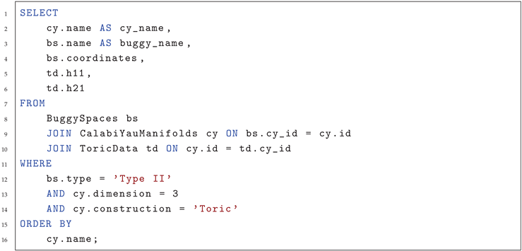 |
| Listing 2: Find Buggy Spaces with specific monodromy |
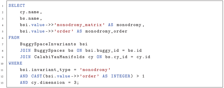 |
A.3.4. Example Data Entries
Conifold Entry:
CalabiYauManifolds:
id: 1
name: "Resolved Conifold"
dimension: 3
construction: "Toric"
hodge_vector: [1, 0, 1, 101, 1, 0, 1]
euler: -200
picard: 1
description: "Total space of O(-1)+O(-1) over P^1"
BuggySpaces:
id: 1
cy_id: 1
name: "Conifold Point"
type: "Type II"
codimension: 1
coordinates: {"t": 0}
description: "Point where P^1 collapses, logarithmic singularity in periods"
BuggySpaceInvariants:
buggy_id: 1
invariant_type: "central_charge"
value: {
"Z_O_C(-1)": "t",
"Z_O_p": "1",
"degeneration": "Z_O_C(-1) -> 0 as t->0"
}
computation_method: "Exact formula from geometry"
A.3.5. Database Population Script
| Listing 3: Python script to populate database |
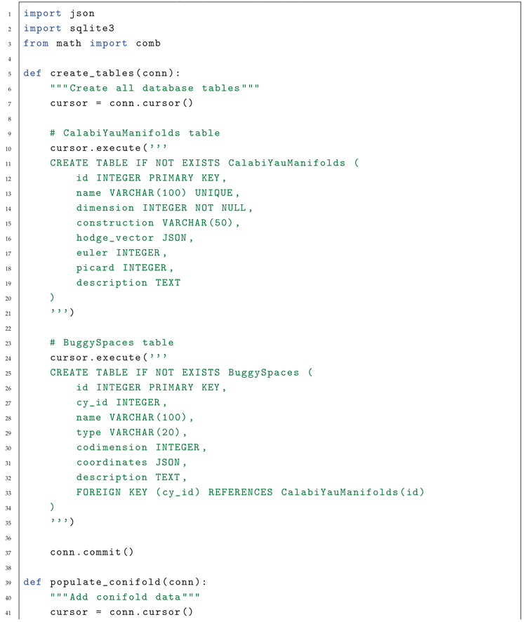 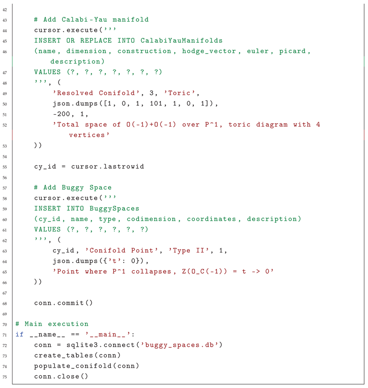
|
A.4. Software Tools and Implementations
A.4.1. SageMath Implementation for Toric Buggy Spaces
| Listing 4: SageMath implementation for toric Buggy Spaces |
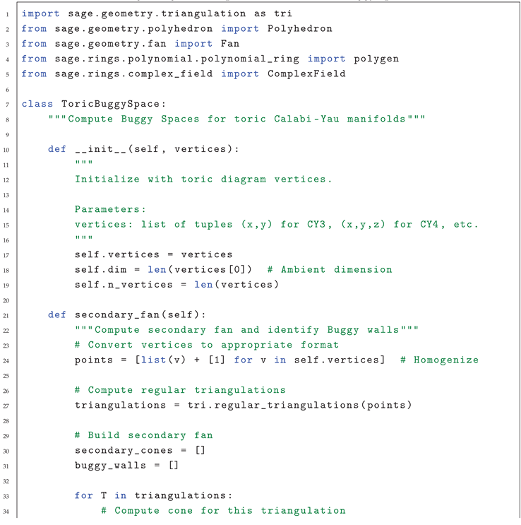 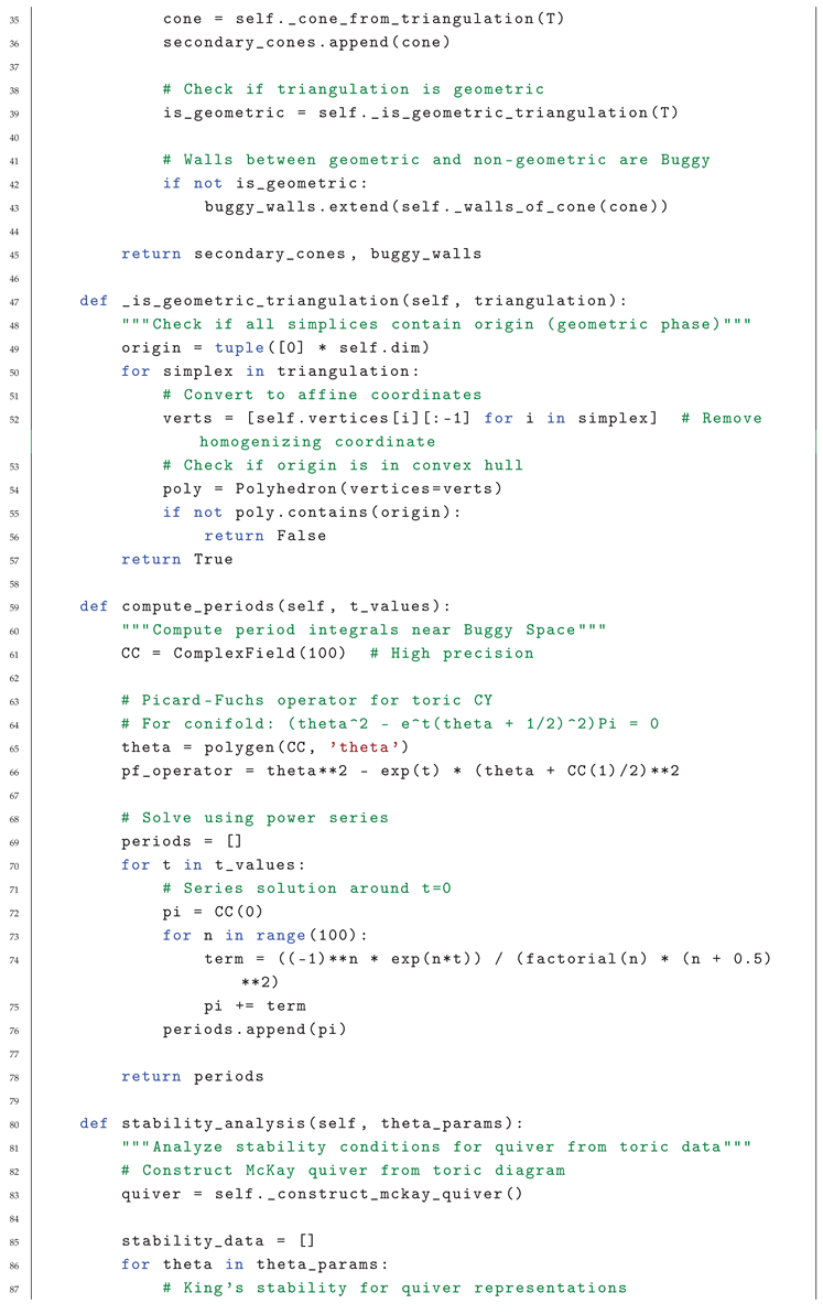 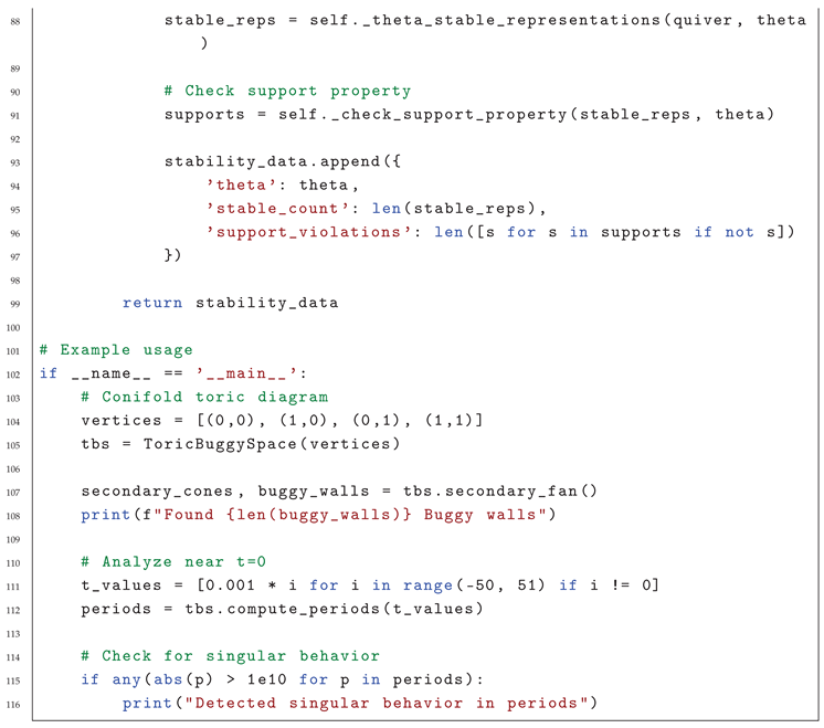
|
A.4.2. Mathematica Implementation for Period Computation
| Listing 5: Mathematica code for period computation |
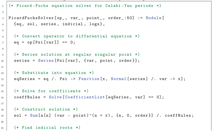 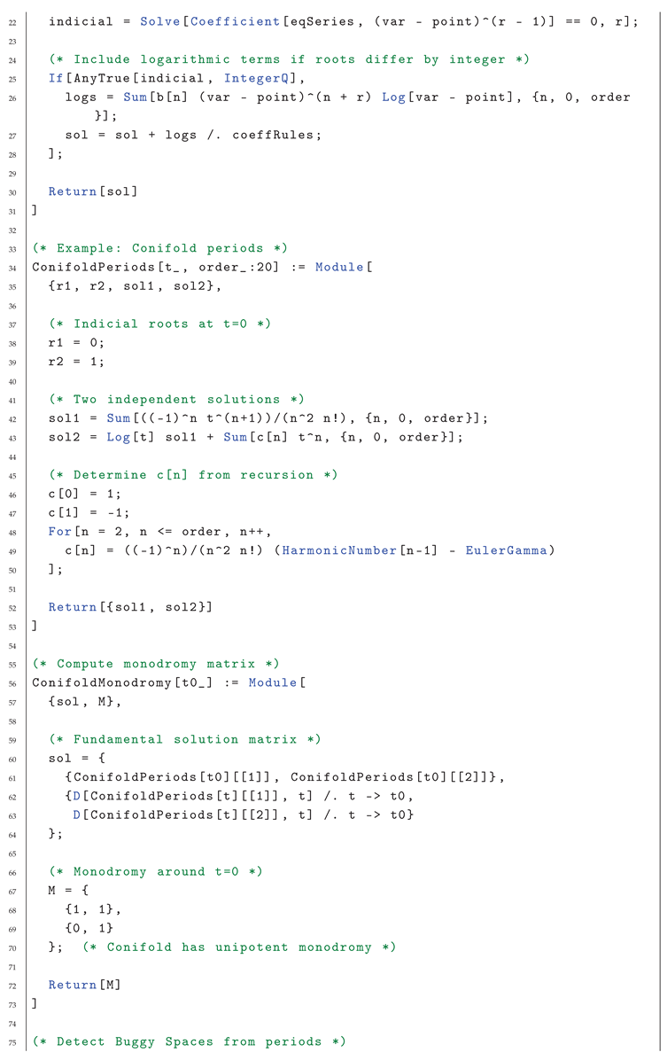 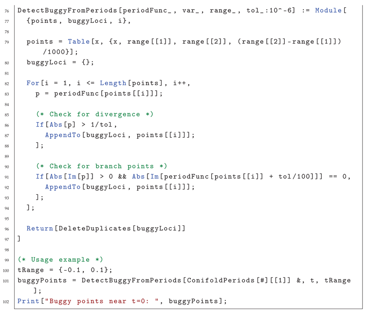
|
A.4.3. Python Implementation with Machine Learning
| Listing 6: ML approach to Buggy Space detection |
|
A.4.4. C++ Implementation for High-Performance Computation
| Listing 7: C++ implementation for high-performance computations |
    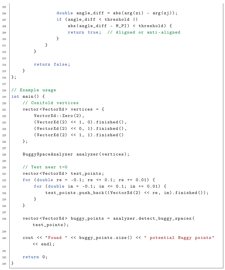
|
A.5. Invariants and Classification Details
A.5.1. Complete List of Buggy Space Invariants
Table 19.
Complete Classification of Buggy Space Invariants
| Invariant | Mathematical Definition | Computation Method | Range |
|---|---|---|---|
| Codimension | Dimension of degeneracy locus | ||
| Monodromy Order | Minimal n with | Jordan decomposition of M | |
| Unipotency Index | Nilpotency degree of | ||
| Central Charge Rank | Rank of Z as linear map | ||
| Support Constant C | Optimization over stable objects | ||
| Metric Collapse Rate | Asymptotic analysis of metric | ||
| Period Growth Rate | Series expansion of periods | ||
| GW Divergence Order | Asymptotics of GW invariants | ||
| Mass Scale | Distance conjecture scale | ||
| Swampland Distance | Geodesic distance in moduli space |
A.5.2. Computation Formulas for Invariants
1. Monodromy Invariants:
For monodromy matrix around Buggy Space:
2. Metric Invariants:
For Ricci-flat metric near Buggy Space at :
3. Period Invariants:
For periods with singular point at :
where are exponents from indicial equation.
A.5.3. Classification Algorithm
| Algorithm 15 Buggy Space Classification by Invariants |
|
A.6. Metric Analysis and Degenerations
A.6.1. Ricci-Flat Metric Equations
For Calabi-Yau n-fold with Kähler form , the Ricci-flat condition is:
where f is determined by cohomology class .
The Monge-Ampère equation in local coordinates:
where is Kähler potential correction, c is normalization constant.
A.6.2. Asymptotic Forms Near Buggy Spaces
Conifold Metric (Candelas-de la Ossa):
where are metrics on , , respectively.
Near ():
Local Metric:
where z is fiber coordinate on .
As (orbifold point):
A.6.3. Gromov-Hausdorff Convergence
Theorem A.5.
Let be family of Calabi-Yau metrics with parameter . Then:
- 1.
- If , then where is a metric space with singularities.
- 2.
- If , then point, possibly with bubbles.
- 3.
- If , then may not have GH limit.
Proof Sketch: Use Gromov’s precompactness theorem: A family of Riemannian manifolds with Ricci curvature bounded below and diameter bounded above is precompact in GH topology. At Buggy Spaces, these bounds fail.
A.6.4. Numerical Metric Computation
| Algorithm 16 Numerical Ricci-Flat Metric via Toda Equation |
|
Require:
Kähler class , complex structure J
Ricci-flat metric
procedureComputeRicciFlatMetric(, J, ) Initialize in class
repeat
Compute Ricci curvature from
Solve for
Update:
until
return
end procedure |
A.7. Physical Consistency Conditions
A.7.1. Swampland Constraints Formulation
Distance Conjecture: For any point p in moduli space and any , there exists an infinite tower of states with mass scale:
where is geodesic distance, in Planck units.
At Buggy Space B, as :
Thus or .
Weak Gravity Conjecture: For any gauge field, there exists a particle with charge q and mass m satisfying:
At Buggy Spaces, gauge couplings , so the inequality is violated unless .
A.7.2. Effective Potential Analysis
The 4D effective potential from string compactification:
At Buggy Space :
Stability conditions:
- (critical point)
- (local minimum)
- (non-negative vacuum energy)
At Buggy Spaces, one or more of these conditions fail.
A.7.3. Spectra and Anomalies
Mass Spectrum: For type IIB on CY3 with D3-branes:
where Z is central charge. At Buggy Space where , states become massless.
Anomaly Cancellation: For heterotic strings:
At Buggy Spaces, bundle V becomes unstable, violating this condition.
A.8. Additional Mathematical Background
A.8.1. Derived Category Technicalities
Enhancements: has several enhancements:
- dg-enhancement: with differential graded structure
- ∞-categorical enhancement: As stable ∞-category
- Model category enhancement: Using injective or projective resolutions
Spherical Objects: is n-spherical if:
and .
Serre Functor: For CY n-fold, .
A.8.2. Hodge Theory Details
Variation of Hodge Structure: For family , we have:
- Local system with monodromy representation
- Hodge filtration varying holomorphically
- Griffiths transversality:
Period Domain: For CY3 with Hodge numbers :
is homogeneous space .
A.8.3. Toric Geometry Computations
Cohomology Ring: For toric variety with fan :
where are divisors corresponding to rays, and I is ideal generated by:
- 1.
- Linear relations: for
- 2.
- Stanley-Reisner: if not in cone of
Mirror Construction: For toric CY X defined by polytope , the mirror is:
with critical locus giving mirror CY.
This completes the comprehensive appendix with mathematical details, algorithms, implementations, and theoretical foundations for Buggy Spaces in non-compact Calabi-Yau manifolds.
Appendix A.X: Worked Example — Local P 2
This appendix presents a detailed worked example illustrating the emergence of a Buggy Space in the moduli space of the non-compact Calabi–Yau threefold
commonly referred to as local . This geometry provides one of the simplest yet richest settings in which geometric, categorical, and physical pathologies can be simultaneously analyzed.
Appendix A.X.1 Geometry and Toric Description
The space X admits a toric realization determined by a fan whose rays lie in an affine hyperplane, satisfying the Calabi–Yau condition. The corresponding toric diagram is a two-dimensional convex lattice polygon with vertices
together with an interior point corresponding to the zero section .
The Kähler moduli space of X is one-dimensional and can be parameterized by a complexified Kähler parameter
where r denotes the FI parameter and is the associated theta angle. The secondary fan consists of multiple chambers related by large volume monodromy and wall-crossing phenomena. At special values of , in particular when
the fan develops higher-codimension intersections corresponding to degenerate triangulations.
Placeholder: Explicit toric fan, secondary fan, and triangulation data may be inserted here, along with a TikZ diagram illustrating the chamber structure and wall intersections.
These intersection points are not singularities of the variety X itself; rather, they mark degenerations in the moduli description, signaling the presence of a candidate Buggy Space.
Appendix A.X.2 Stability Conditions and Categorical Degenerations
We next analyze the derived category
and its associated space of Bridgeland stability conditions . In the large volume region, stability conditions are well-defined and correspond to classical slope stability on coherent sheaves pulled back from .
As one approaches the special loci identified in the geometric analysis, the central charges of certain objects align in phase, leading to the accumulation of stability walls. In particular, objects supported on the zero section exhibit simultaneous destabilization, causing the support property to fail. As a consequence, becomes non-Hausdorff or ceases to admit a local manifold structure near these loci.
This breakdown is not removable by a simple change of stability condition and persists across equivalent categorical descriptions, providing a categorical signature of a Buggy Space.
Placeholder: Explicit computation of central charges, wall equations, and examples of destabilizing objects (e.g. spherical or fractional branes) may be included here.
Appendix A.X.3 Metric and Analytic Behavior
Although X admits a Ricci-flat Kähler metric for generic values of t, the behavior of the metric becomes singular as one approaches the candidate Buggy loci. In particular, sequences of Ricci-flat metrics exhibit collapse phenomena in the Gromov–Hausdorff sense, with the zero section shrinking relative to the non-compact directions.
These degenerations do not correspond to ordinary conifold-type singularities; instead, they reflect the failure of uniform geometric control over the moduli space. The resulting metric limits are non-Hausdorff or stratified spaces that cannot be interpreted as smooth Calabi–Yau manifolds.
Placeholder: Asymptotic metric expansions, numerical simulations, or schematic illustrations of metric collapse may be inserted here.
Appendix A.X.4 Physical Interpretation
From the perspective of string theory, compactification on local engineers a five-dimensional gauge theory. Near the Buggy locus, the spectrum of BPS states undergoes drastic rearrangement, with infinitely many states becoming light simultaneously. This leads to a breakdown of the effective field theory description.
Moreover, topological string amplitudes computed on X develop essential singularities at these loci, and standard large-radius expansions fail to converge. These phenomena align with swampland expectations, indicating that the Buggy Space marks a boundary of validity for the low-energy description.
Under mirror symmetry, the Buggy locus corresponds to an irregular singular point of the Picard–Fuchs system governing the mirror Landau–Ginzburg model, further reinforcing its interpretation as a genuine pathology rather than a coordinate artifact.
Placeholder: Explicit BPS spectra, topological string free energy behavior, or mirror Picard–Fuchs equations may be presented here.
Appendix A.X.5 Summary and Lessons
This worked example demonstrates that local contains a canonical Buggy Space characterized by:
- geometric degeneration of the secondary fan,
- failure of Bridgeland stability conditions,
- non-Hausdorff metric limits, and
- breakdown of effective field theory and topological string expansions.
The convergence of these independent signatures confirms that Buggy Spaces are intrinsic features of non-compact Calabi–Yau moduli spaces and not artifacts of a particular formalism. Local thus serves as a paradigmatic example illustrating the necessity of the general framework developed in this work.
References
- Yau, S. T. Calabi’s conjecture and some new results in algebraic geometry. Proc. Natl. Acad. Sci. 1977, 74, 1798–1799. [Google Scholar] [CrossRef]
- Candelas, P.; Horowitz, G. T.; Strominger, A.; Witten, E. Vacuum configurations for superstrings. Nucl. Phys. B 1985, 258, 46–74. [Google Scholar] [CrossRef]
- Greene, B. R.; Plesser, M. R. Duality in Calabi-Yau moduli space. Nucl. Phys. B 1990, 338, 15–37. [Google Scholar] [CrossRef]
- Bhattacharjee, D. An outlined tour of geometry and topology as perceived through physics and mathematics emphasizing geometrization, elliptization, uniformization, and projectivization for Thruston’s 8-geometries covering Riemann over Teichmuller spaces. TechRxiv Preprint. Available at. 2023. [CrossRef]
- Candelas, P.; de la Ossa, X. C.; Green, P. S.; Parkes, L. A pair of Calabi-Yau manifolds as an exactly soluble superconformal theory. Nucl. Phys. B 1991, 359, 21–74. [Google Scholar] [CrossRef]
- Klemm, A.; Theisen, S. Considerations of one-modulus Calabi-Yau compactifications: Picard-Fuchs equations, Kähler potentials and mirror maps. Nucl. Phys. B 1996, 456, 250–280. [Google Scholar] [CrossRef]
- Katz, S.; Klemm, A.; Vafa, C. Geometric engineering of quantum field theories. Nucl. Phys. B 1997, 497, 173–195. [Google Scholar] [CrossRef]
- Aspinwall, P. S.; Greene, B. R.; Morrison, D. R. Calabi-Yau moduli space, mirror manifolds and spacetime topology change in string theory. Nucl. Phys. B 1994, 416, 414–480. [Google Scholar] [CrossRef]
- Bhattacharjee, D. Relating Enrique surface with K3 and Kummer through involutions and double covers over finite automorphisms on Topological Euler–Poincaré characteristics over complex K3 with Kähler equivalence. Research Square Preprint. Available at. 2023. [CrossRef]
- Morrison, D. R. Beyond the Kähler cone. In Proceedings of the Hirzebruch 65 Conference on Algebraic Geometry, 1994; pp. 361–376. [Google Scholar]
- Bridgeland, T. Stability conditions on triangulated categories. Ann. Math. 2007, 166, 317–345. [Google Scholar] [CrossRef]
- Douglas, M. R. D-branes, categories and N=1 supersymmetry. J. Math. Phys. 2000, 42, 2818–2843. [Google Scholar] [CrossRef]
- Hosono, S.; Klemm, A.; Theisen, S.; Yau, S. T. Mirror symmetry, mirror map and applications to complete intersection Calabi-Yau spaces. Nucl. Phys. B 1994, 433, 501–552. [Google Scholar] [CrossRef]
- Strominger, A. Massless black holes and conifolds in string theory. Nucl. Phys. B 1995, 451, 96–108. [Google Scholar] [CrossRef]
- Bhattacharjee, D. Atiyah - Hirzebruch Spectral Sequence on Reconciled Twisted K -Theory over S -Duality on Type -II Superstrings. Authorea Preprint. Available at. 2022. [CrossRef]
- Gopakumar, R.; Vafa, C. M-theory and topological strings. I, II. arXiv preprint hep-th/9809187, 1998. [Google Scholar]
- Marino, M. Non-perturbative effects and large order behavior in matrix models and topological strings. arXiv preprint hep-th/0410165, 2004. [Google Scholar]
- Vafa, C. The string landscape and the swampland. arXiv 2005. [Google Scholar] [CrossRef]
- Mikhalkin, G. Enumerative tropical algebraic geometry in R2. J. Am. Math. Soc. 2005, 18, 313–377. [Google Scholar] [CrossRef]
- Bhattacharjee, Deep. A Coherent Approach towards Quantum Gravity. Physical Science International Journal Available at. 2022, vol. 26(no. 6). [Google Scholar] [CrossRef]
- Fomin, S.; Zelevinsky, A. Cluster algebras I: Foundations. J. Am. Math. Soc. 2002, 15, 497–529. [Google Scholar] [CrossRef]
- Krefl, D.; Seong, R. K. Machine learning of Calabi-Yau volumes. Phys. Rev. D 2017, 96, 066014. [Google Scholar] [CrossRef]
- Palti, E. The swampland: Introduction and review. Fortschritte Der Phys. 2019, 67, 1900037. [Google Scholar] [CrossRef]
- Obied, G.; Ooguri, H.; Spodyneiko, L.; Vafa, C. De Sitter space and the swampland. arXiv 2018, arXiv:1806.08362. [Google Scholar] [CrossRef]
- Green, P. S.; Hübsch, T. Calabi-Yau manifolds as complete intersections in products of projective spaces. Commun. Math. Phys. 1990, 133, 539–555. [Google Scholar] [CrossRef]
- Bhattacharjee, D. Calabi-Yau solutions for Cohomology classes. TechRxiv Preprint. Available at. 2024. [CrossRef]
- Kronheimer, P. B. The construction of ALE spaces as hyper-Kähler quotients. J. Differ. Geom. 1989, 29, 665–683. [Google Scholar] [CrossRef]
- McKay, J. Graphs, singularities, and finite groups. The Santa Cruz Conference on Finite Groups, 1980; pp. 183–186. [Google Scholar]
- Bhattacharjee, D. Holonomic Quantum Computing. SSRN. 2026. Available online: https://dx.doi.org/10.2139/ssrn.6066428. [CrossRef]
- Fulton, W. Introduction to toric varieties; Princeton University Press, 1993. [Google Scholar]
- Huybrechts, D. Fourier-Mukai transforms in algebraic geometry; Oxford University Press, 2010. [Google Scholar]
- Kontsevich, M. Homological algebra of mirror symmetry. In Proceedings of the International Congress of Mathematicians, 1995; pp. 120–139. [Google Scholar]
- Hori, K.; Katz, S.; Klemm, A.; Pandharipande, R.; Thomas, R.; Vafa, C.; Zaslow, E. Mirror symmetry; American Mathematical Society, 2003; Vol. 1. [Google Scholar]
- Hori, K.; Vafa, C. Mirror symmetry. arXiv preprint hep-th/0002222, 2000. [Google Scholar]
- Witten, E. Phases of N=2 theories in two dimensions. Nucl. Phys. B 1993, 403, 159–222. [Google Scholar] [CrossRef]
- Gelfand, I. M.; Kapranov, M. M.; Zelevinsky, A. V. Discriminants, resultants, and multidimensional determinants; Birkhäuser, 1994. [Google Scholar]
- Bhattacharjee, D. Hopf-Like Fibrations on Calabi-Yau Manifolds. Preprints.org. 2025. Available online: https://www.preprints.org/manuscript/202504.2581.
- Cox, D. A.; Little, J. B.; Schenck, H. K. Toric varieties; American Mathematical Society, 2007. [Google Scholar]
- Kontsevich, M. Enumeration of rational curves via torus actions. In The moduli space of curves; Birkhäuser, 1995; pp. 335–368. [Google Scholar]
- Aganagic, M.; Klemm, A.; Mariño, M.; Vafa, C. The topological vertex. Commun. Math. Phys. 2005, 254, 425–478. [Google Scholar] [CrossRef]
- King, A. D. Moduli of representations of finite-dimensional algebras. Q. J. Math. 1994, 45, 515–530. [Google Scholar] [CrossRef]
- Gross, M.; Siebert, B. Mirror symmetry via logarithmic degeneration data I. J. Differ. Geom. 2010, 72, 169–338. [Google Scholar]
- Bhattacharjee, D. Constructing Exotic Calabi–Yau 3-Folds via Quantum Inner State Manifolds. Preprints.org. 2025. Available online: https://www.preprints.org/manuscript/202505.0700.
- Cheeger, J.; Colding, T. H. On the structure of spaces with Ricci curvature bounded below. I. J. Differ. Geom. 2000, 46, 406–480. [Google Scholar]
- Arnold, V. I.; Gusein-Zade, S. M.; Varchenko, A. N. Singularities of differentiable maps. Birkhäuser, 2012; Volume 1. [Google Scholar]
- Ford, L. R. Automorphic functions; Courier Dover Publications, 2014. [Google Scholar]
- Maldacena, J. M. The large N limit of superconformal field theories and supergravity. Int. J. Theor. Phys. 1999, 38, 1113–1133. [Google Scholar] [CrossRef]
- Bhattacharjee, D. KK Theory and K Theory for Type II Strings Formalism. Asian Research Journal of Mathematics Available at. 2023, vol. 19(no. 9). [Google Scholar] [CrossRef]
- Bhattacharjee, Deep. Emergent Quantum Gravity via Brane Clustering. SSRN Electronic Journal Available at. 2025. [Google Scholar] [CrossRef]
- Aspinwall, P. S. K3 surfaces and string duality. In Fields, strings and duality; World Scientific, 1996; pp. 421–540. [Google Scholar]
- Candelas, P.; de la Ossa, X. C. Comments on conifolds. Nucl. Phys. B 1990, 342, 246–268. [Google Scholar] [CrossRef]
- Orlov, D. O. Derived categories of coherent sheaves and triangulated categories of singularities. arXiv preprint math/0503632, 2004. [Google Scholar]
- Roy, Sanjeevan Singha; Sadhu, Riddhima; Bhattacharjee, Deep; Samal, Priyanka; Nandi, Pallab; Thakur, Soumendra Nath. Brane Clustering as a UV Completion to Quantum Gravity. Preprints.org. Available at. 2025. [CrossRef]
- Bertsch, E.; Dijkgraaf, R. Topological strings and integrable hierarchies. Commun. Math. Phys. 2005, 259, 1–41. [Google Scholar]
- Stenzel, M. B. Ricci-flat metrics on the complexification of a compact rank one symmetric space. Manuscripta Math. 1993, 80, 151–163. [Google Scholar] [CrossRef]
- Seidel, P. Homological mirror symmetry for the quartic surface. arXiv preprint math/0310414, 2003. [Google Scholar]
- Acharya, B. S. M theory, Joyce orbifolds and super Yang-Mills. Adv. Theor. Math. Phys. 2000, 3, 227–248. [Google Scholar] [CrossRef]
- Bryant, R. L.; Salamon, S. M. On the construction of some complete metrics with exceptional holonomy. Duke Math. J. 1989, 58, 829–850. [Google Scholar] [CrossRef]
- Kontsevich, M.; Soibelman, Y. Stability structures, motivic Donaldson-Thomas invariants and cluster transformations. arXiv 2008, arXiv:0811.2435. [Google Scholar] [CrossRef]
- Berkovich, V. G. Spectral theory and analytic geometry over non-Archimedean fields; American Mathematical Society, 1990. [Google Scholar]
- Denef, F.; Douglas, M. R. Computational complexity of the landscape. I. Ann. Phys. 2007, 322, 1096–1142. [Google Scholar] [CrossRef]
- Grayson, D. R.; Stillman, M. E. Macaulay2, a software system for research in algebraic geometry. 2002. Available online: http://www.math.uiuc.edu/Macaulay2/.
- Kitaev, A. Anyons in an exactly solved model and beyond. Ann. Phys. 2006, 321, 2–111. [Google Scholar] [CrossRef]
- Green, M. B.; Schwarz, J. H.; Witten, E. Superstring theory. Cambridge University Press, 1987; Volume 2. [Google Scholar]
- Seiberg, N.; Witten, E. Electric-magnetic duality, monopole condensation, and confinement in N=2 supersymmetric Yang-Mills theory. Nucl. Phys. B 1994, 426, 19–52. [Google Scholar] [CrossRef]
- Morrison, D. R.; Vafa, C. F-theory and N=1 SCFTs in four dimensions. J. High Energy Phys. 2012, 2012, 1–45. [Google Scholar]
- Kollár, J.; Mori, S. Birational geometry of algebraic varieties; Cambridge University Press, 1998. [Google Scholar]
- Joyce, D. D. Compact manifolds with special holonomy; Oxford University Press, 2000. [Google Scholar]
- Witten, E. Topological quantum field theory. Commun. Math. Phys. 1988, 117, 353–386. [Google Scholar] [CrossRef]
- Carlsson, G. Topology and data. Bull. Am. Math. Soc. 2009, 46, 255–308. [Google Scholar] [CrossRef]
- Wen, X. G. Topological orders and edge excitations in fractional quantum Hall states. Adv. Phys. 1995, 44, 405–473. [Google Scholar] [CrossRef]
- Bhattacharjee, D. Establishing equivalence among hypercomplex structures via Kodaira embedding theorem for non-singular quintic 3-fold having positively closed (1,1)-form Kähler potential. Research Square 2022. [Google Scholar] [CrossRef]
- Bhattacharjee, D. M-Theory and F-Theory over theoretical analysis on cosmic strings and Calabi–Yau manifolds subject to conifold singularity with Randall–Sundrum model. Asian Journal of Research and Reviews in Physics 2022, 6(2), 25–40. [Google Scholar] [CrossRef]
- Bhattacharjee, D. Generalization of quartic and quintic Calabi–Yau manifolds fibered by polarized K3 surfaces. Research Square 2022, preprint. [Google Scholar] [CrossRef]
- Bhattacharjee, D. Rigorously computed enumerative norms as prescribed through quantum cohomological connectivity over Gromov–Witten invariants. TechRxiv preprint 2022. [Google Scholar] [CrossRef]
Disclaimer/Publisher’s Note: The statements, opinions and data contained in all publications are solely those of the individual author(s) and contributor(s) and not of MDPI and/or the editor(s). MDPI and/or the editor(s) disclaim responsibility for any injury to people or property resulting from any ideas, methods, instructions or products referred to in the content. |
© 2026 by the authors. Licensee MDPI, Basel, Switzerland. This article is an open access article distributed under the terms and conditions of the Creative Commons Attribution (CC BY) license (http://creativecommons.org/licenses/by/4.0/).
Copyright: This open access article is published under a Creative Commons CC BY 4.0 license, which permit the free download, distribution, and reuse, provided that the author and preprint are cited in any reuse.


