
Submitted:
26 January 2026
Posted:
27 January 2026
You are already at the latest version
Abstract
Gas emissions containing particulate matter are the most prevalent in technological processes. To reduce emissions into the atmosphere, it is necessary to apply gas pre-treatment before high-efficiency filters, which in interaction helps to achieve a favorable result for reducing the level of fine and ultrafine particles particularly dangerous to the human health. Electric field manipulator (agglomerator) can influence these fine particulate matter and results in an increase in their size. Comprehensive aerodynamic study aim to elucidate the gas flow distribution, variation of trajectories and dynamics at different flow rates, specifically the trajectories and velocities of particles within the gas flow. These factors provide meaningful assumptions about the possible behavior of particles in the flow and there are critical for optimizing an agglomeration and its intensity. Such phenomena can have an impact on the probability of agglomeration in the manipulator channels, i.e., the sticking of small particles into larger ones, and this allows improving the design and operating conditions of the apparatus. Gas flow velocities and pressure were analyzed experimentally at various cross-sectional points in the inlet and outlet ducts at the inflow rate of 3.4-50 l/s. Pressure-based solver with the coupled scheme for pressure-velocity coupling was used. The static pressure at the inlet of manipulator varied from 8 to 178 Pa. This study provides new insights into flow pre-treatment using the electric field mechanism in a multichannel modular apparatus and provides a reasonable understanding of the necessary characteristics of the gas flow distribution for its subsequent improvement for highest agglomeration.
Keywords:
gas flow
; particles
; electric field
; agglomeration
; aerodynamics
1. Introduction
Conventional treatment technologies, which utilize principles such as gravity, centrifugal force, and electrostatics, are widely employed for the elimination of particulate matter (PM). While these methods effectively remove particles larger than 1 µm, their efficiency in capturing finer particles from the gas flow is limited, particularly considering proposed emission limits and the urgent need to reduce future pollution. The Euro 7 standard is the upcoming European regulation on vehicle emissions, expected to apply stricter limits on exhaust emission including the number of exhaust particles at the level of PN10, instead of PN23, i.e., particle number of 23 μm.
Particulate matter, including fine and ultrafine particles (UFPM), poses significant risks to both human health and the natural environment [1,2,3].
Particulate matter (PM) is a mixture of particles and liquid droplets (aerosols) in the air, which can contain various components such as acids, sulfates, nitrates, organic compounds, metals, soil particles, dust, soot and etc. The solid particles emitted into the air exhibit significant variation in their physical and chemical composition, particle sizes, and sources of emission [4].
The most painful effects are caused by solid particles from 10-0.1 µm. Once inhaled, these particles can settle in various parts of the respiratory system. Larger particles tend to deposit in the upper airways, while ultrafine particles can reach the peripheral regions of the lungs, including the alveoli. From there, they can even enter the bloodstream and circulate throughout the body, potentially causing various health issues. Lung-deposited surface area (LDSA) refers to the total surface area of airborne particles that can be deposited onto the lung’s respiratory tract, particularly in the alveolar and bronchiolar regions. Unlike measuring particle concentration based on mass or number, LDSA considers the effective surface area of particles that come into contact with lung tissue, which is a crucial factor in assessing health risks related to ultrafine particles (particles smaller than 100 nm) [5].
Additionally, current technologies struggle with adaptability and effectiveness when managing a wide range of particulate matter (PM) concentrations within the flow. Furthermore, these filtration systems tend to clog quickly [6]. This often necessitates pre-treatment or specialized handling of contaminated gas flows. Moreover, current technologies are inadequate or inefficient when dealing with a broad spectrum or elevated levels of particulate matter (PM) flow. Consequently, pre-treatment or specialized treatment of the contaminated flow becomes essential. The use of these technologies as standalone treatment units is also limited, requiring careful consideration of PM type and characteristics, as well as gas flow properties [7,8].
Small particles can agglomerate through several processes. Despite their small diameters, strong forces such as Van der Waals interactions, electrostatic forces, and capillary forces act between these particles. Collectively, these forces create an attractive force, allowing the particles to form larger compounds [9].
Agglomeration of particulate matter can occur due to various forms of particle interactions, which can be grouped into solid bridges, mobile liquid binding, intermolecular and electrostatic forces, and mechanical interlocking. Solid bridges may form through sintering, crystallization, or with the aid of bonding agents like resins. The driving forces behind mobile liquid binding include interfacial forces and capillary suction, with the bond strength depending on the binder’s properties. Intermolecular and electrostatic forces act between particulate matter without the formation of material bridges. These forces are more prominent in smaller particles, as gravitational forces tend to dominate in larger particles. Mechanical interlocking occurs due to the geometrical properties of the particles. During mixing processes, particles can become entangled and accumulate into larger agglomerates [10].
The most used methods to apply these mechanisms to particulate matter are chemical agglomeration, ultrasonic agglomeration and electrostatic agglomeration.
Chemicals can be used to induce agglomeration in PM. Therefore, chemical agglomerants are directly sprayed into the flow to be cleaned gas stream [11,12].
An effective method for particle agglomeration is the application of sound waves on PM, known as ultrasonic agglomeration. In addition to orthokinetic interactions, ultrasonic agglomeration at frequencies ranging from 16 kHz to 1 MHz can also make use of ultrasonic cavitation. This phenomenon enhances particle collisions and interactions, leading to the growth of particle size. Furthermore, ultrasonic waves can reduce surface charges to eliminate electrostatic repulsion and increase surface energy which improves adhesion of particles [13].
The application of an electric field is important for the study of flow electro hydrodynamics. The work [14] deals with devices with electro convective flow, which is induced by so-called charge spray. Such technology is used for the micro-mixing of liquids as well as for their atomization. Unipolar electric fields are mainly applied to alternating currents with a sinusoidal phase, but changes in alternating and pulsed electric fields and the transition from DC to AC are also investigated. In the case of a unipolar field, the charge carriers are usually assumed to be electrons and positive, so the electric potential is calculated using Poisson’s equation, which takes into account the charge density [15].
Electrostatic agglomerators can be categorized into two main groups [16]. A bipolar agglomerator typically consists of a charging section and an electric field section. In the charging section, the gas stream is split into two halves, and a corona discharge is used to polarize each of these streams with opposite polarities. As the charged gas streams enter the electric field section, the particles collide due to Coulomb attraction forces. The motion of these particles can be described by the Equation (1) [17]:
here, q is the charge of the particle, E is the intensity of the electric field, m is the particle mass, and µ is the gas viscosity. It should be noted that both electrical parameters as well as properties of the particles influence the agglomeration process.
Equation 2 describes the time-dependent increase in the particle charge qp of a spherical particle with a diameter dp:
Key influencing factors include the ion concentration in the charging zone ci, the mobility of the gaseous ions bi, the relative permittivity of the particles εr, the electric field constant ε0 and the elementary charge e. The only actively controllable parameter is the electric field strength E.
As the particle charge increases, a Coulomb repulsion force develops, preventing further charge accumulation. This results in a saturation limit, known as the Pauthenier limit, with the saturation charge Qs, which can be determined using the Pauthenier equation (Equation 3):
It follows that the saturation charge depends only on the electric field and is independent of the ion concentration.
The second mechanism, diffusion charging, occurs through collisions between ions and particles due to Brownian motion. Temperature is a crucial factor, as it significantly influences the mean kinetic energy of the ions. Here, too, an Equation 4 is used to describe the charge increase over time:
As previously mentioned, this introduces the root mean square velocity ¯ vi, which depends on the kinetic energy according to Maxwell-Boltzmann statistics, the Boltzmann constant k, and the absolute temperature T in K.
Like the bipolar agglomerator, a unipolar agglomerator also consists of a charging section and an agglomeration section. However, in this case, the gas stream is not separated, and the entire stream is charged with the same polarity. In the agglomeration section, an alternating electric field is used to induce oscillatory motion, forcing the particles to collide and agglomerate. The difference in velocity and amplitude of the oscillatory movement between larger and smaller particles is the primary cause of collisions [18].
Understanding the motion and velocities of particles in a gas stream is crucial as these factors determine the probability of particle collisions, at the same time the frequency and efficiency of such a phenomenon, as well as the subsequent agglomeration of both primary and secondary agglomeration. The application of a forced electric field in air channels can change the trajectories of charged particles, also called general ion wind flow. The distribution of air flow velocity from the entrance to the distribution system of channels, available local barriers, where the flow pressure drop occurs, have a direct impact on the particle dynamics, and hence on the agglomeration efficiency [19]. In the study [20], electro-vortex technology was investigated to improve particle capture efficiency. The importance of the combination of mechanisms is to direct the particles in the desired trajectory, to create conditions in which the particles stay long enough in the electric field for their agglomeration, but also not to create excessive pressure losses, but on the contrary to stabilize the particle motion and reduce velocity fluctuations, which leads to a more homogeneous distribution of particles and improved agglomeration.
Particle charging occurs according to two mechanisms, i.e., field charging and diffusion charging. Similar to agglomeration, electrostatic precipitation utilizes the corona effect, which ionizes surrounding gas molecules near the discharge electrode. Due to the electrical permittivity of the particles, the electric field lines concentrate around the particles. Ions following these field lines collide with the particles, leading to a process known as field charging. Another mechanism contributing to particle charging is diffusion charging, where Brownian motion causes collisions between particles and ions in the surrounding gas. These charging effects facilitate the transfer of charge from the ions to the particles until a saturation limit is reached [21]. Diffusion charging occurs when ions collide with airborne particles due to Brownian motion [22]. In contrast, field charging requires an external electric field that moves the ions along the field lines, causing them to collide with the particles along their path. The ion flux is correlated with ion mobility Z and the electric field strength E, which therefore influences particle charging. Additionally, particle properties such as the dielectric constant K and the saturation charge of the particles also play a role in this process [23]. The space between the electrodes can be divided into two regions: the ionization region and the drift region. The ionization region is relatively small, with high electric field strengths prevailing due to the asymmetric field geometry. In this region, free electrons are strongly accelerated by the high field strength and move toward the ground electrode. Their acceleration is sufficient to ionize atoms and molecules upon collision, resulting in the release of additional electrons and the formation of positive ions. In the drift region, the energy of the electrons is no longer sufficient to ionize additional atoms, as the electric field strength has decreased significantly. Instead, free electrons attach to gas molecules, forming negatively charged ions. These ions migrate toward the collecting electrode due to electrostatic attraction. Two additional effects occur during corona discharge. First, when electrons are released from their atomic orbitals, photons are emitted, which are visible as a glow. However, this glow does not extend from one electrode to the other but terminates within the ionization region. Second, the movement of negatively charged gas ions toward the collecting electrode generates an airflow, known as the corona wind [24].
Research [25] was presented some aerodynamic phenomena into the electric field. One of the findings is that processes are less intensive at low flow velocities or in high-volume ducts, the electric field and its various properties significantly impact the flow state. At a peak voltage of 45 kV and a pulse frequency of 20 kHz, the efficiency increased when the gas velocity was raised from 0.5 m/s to 1 m/s. However, a lower efficiency was observed when the velocity exceeded 1 m/s. Under these conditions, the sub-micron particle number reduction efficiency for all particle sizes exceeded 90% in the non-thermal plasma ESP. To tackle these challenges, one effective strategy is the agglomeration method. By deliberately enlarging particle size through forced means, the modified quantitative and qualitative properties of the particles allow for the use of standard cleaning techniques or achieve a higher level of cleaning. Importantly, the relaxation movements of particles caused by the generated electric field are essential to this agglomeration process [26].
To maintain air quality, especially in rooms where people spend long periods of time, it is necessary to rationally solve the problem of dust from both natural and man-made sources. People are increasingly spending time in enclosed spaces such as administrative buildings, as well as temporary spaces such as airport waiting rooms, movie theaters, etc. High-efficiency filters (HEPA, ULPA) are used to precipitate micron particles with sufficient efficiency, but these filters are not effective enough at trapping submicron and nanoscale particles due to their structure [27]. Ultra-fine particles are concentrated and thus constitute the predominant fraction in the entire air content, and with multiple sources, the probability of them entering the human respiratory zone increases. Pretreatment of the contaminated flow facilitates the purification process, makes it more economical, and selectively acts on the smallest particles for agglomeration, allowing the use of already known technologies with the best flow characteristics. Various scenarios for the volume flow rate of the purified air flow in this study indicate critical phenomena in the agglomeration process and the distribution of trajectories in this device, thereby predetermining their potential area of application and operating modes. The digital model created on the basis of the physical test bench reflects the main trends of the processes. It also allows identifying possible areas for design improvement to achieve the best impact on particles and subject them to effective agglomeration under various conditions.
The objective of this research is to perform an analytical analysis using physical and simulation experiments results, as well as identify a flow distribution within the agglomerator chamber and influence of airflow rate on flow trajectory changes. A comparative analysis of gas flow dynamics in different sections of the bipolar electric field manipulator chamber was carried out to select the qualitative characteristics of the apparatus for ultrafine particle agglomeration.
2. Materials and Methods
2.1. Experimental Setup
Physical experiments were performed in VilniusTech laboratories, the simulations were performed at a National Sun Yat-sen university. For experimental studies on the dynamic limits of gas flow and pressure at laboratory, a specialized research bench was employed. This bench includes a fan, airflow velocity meters at both the inlet and outlet, static pressure meters at the inlet and outlet, an agglomeration chamber, and a fan control unit. The total length of the bench is 2.6 meters, with the agglomeration apparatus measuring 340 mm. Figure 1 provides a schematic representation of the research bench. All measurement guidelines were followed in accordance with the recommended standardized methodology for the experimental study.
The design and electrical circuit of the agglomerator system were created to transfer the necessary critical charge from the electrode plane, as the source of the electric field, to the particle in each of the channels of the manipulator cassette. To create the necessary charge, also known as the saturation charge qsat, a particle with a radius r must be in an electric field with a strength Ecrit. For microparticles, this value is usually taken to be 3×10⁶ V/m, based on which the necessary distance between the electrode planes can be calculated using Equation 5:
here, ε0 – electrical constant.
At present, the manipulator technology is in the patenting stage, so information is partially limited in this work. However, a national patent has already been obtained and a European patent application is being considered, which describe in more detail the principle of operation and design characteristics of the manipulator [28,29].
The gas enters from the inlet of the bench and exits from the outlet, establishing a controlled flow environment. A notable feature of the setup is the equalizing section near the fan (Same sky CFM-80BF-2130-631), which minimizes turbulence as the gas flows into the agglomeration chamber, resulting in a stable gas flow. The system is managed via a control unit that allows for adjustments to the agglomeration chamber’s voltage and the gas flow rate, expressed as a percentage of the nominal flow. This setup provides precise control over experimental conditions, facilitating the observation of the effects of flow rates and electrical charges on particle agglomeration Figure 1. All elements of the air ducts were grounded, including the metal elements of the parameter measurement devices for safety reasons, as well as all tubes used for collecting particle samples to reduce the accumulation of particles due to static charge.
Experimental research was carried out at microclimate conditions typically observed inside the apparatus during the study, temperature was 22.4–22.8 °C and relative humidity was 28.2–28.6%.
Gas flow velocity was recorded at five distinct cross-sectional points at both the inlet (A-E) and outlet (A1-E1) before and after the agglomeration chamber, as illustrated in Figure 1 and Figure 2. The duct features an inner diameter of 148 mm. Velocity measurement probes were inserted through the center of the duct, aligned with both horizontal and vertical planes, and positioned 5 mm from the inner wall, as shown in Figure 2b. Gas flow rate measurements were conducted over a 60-second period, with data collected every second. It was determined that the speed and pressure sensors alter the flow dynamics by no more than 2%, so it was decided to disregard these errors as insignificant.
The fan starts spinning once it reaches 6% efficiency. By adjusting the gas load the measurements were taken at 10%, 50%, and 100%. All test results were recorded using the “testo 440 dP” and “testo 440” measuring devices. Technical data of the multimeter (are the same for both): measuring range 0–50 m/s, -20– +70 °C, 5–95%RH, 700–1100 hPa; accuracy ±(0.03 m/s + 4% of the measuring value (m.v.)) (0 to 20 m/s), ±0.5 °C (0 to +70 °C), ±3.0%RH (10 to 35%RH) and ±2.0%RH (35 to 65%RH), ±3 hPa; resolution 0.01 m/s, 0.1 °C, 0.1%RH, 0.1 hPa.
Static pressure measurements were conducted before and after the agglomeration chamber, specifically at points D and D1 as shown in Figure 2a. The “testo 440 dP” pressure measuring device was used for these measurements. Static pressure readings were taken at 10% intervals from 10% to 100%. Each static pressure measurement lasted 60 seconds, with data collected every second.
Aerodynamic resistance measurements were subsequently performed between the inlet point D and the outlet point D1 in the middle of the duct. These measurements also lasted 60 seconds, with data collected every second.
The agglomeration chamber is segmented into four cross sections, labeled A-A through D-D, as depicted in Figure 3. Each section contains specific measuring points, also shown in Figure 3. Cross section A-A is solely used for measuring static pressure. Cross sections B-B through D-D correspond to the top, middle, and bottom of the multi-layer plate modular cassette. The distances from the top of the chamber (A-A) to the other cross sections are indicated in Figure 3a in millimeters. The chamber is designed to direct gas flow through the plates and the electric field before exiting. During these measurements, the gas flow load was set to 10%, 50%, and 100%. For further distribution of results, cases and measurement points were numbered in this way, e.g., A50, it is inlet point at 50% of the gas flow load, A1 100, it is outlet point at 100% of etc. A total of 800 data points were collected just over one minute. No voltage was applied to the plates during the experiment, so no electric field was generated. Figure 3a shows cross sections with the location and numbering of flow velocity measurement points in the agglomeration chamber; the cross-section level is indicated in part of Figure 3a. The physical location of the samples is shown in Figure 3c.
The gas velocity was measured using the eATVS-8™ automatic temperature and velocity scanner (Advanced Thermal Solutions, Inc., USA). This system, integrated with the setup, enables simultaneous gas velocity measurements at four points. According to the data sheet, the velocity range is from 0 m/s to 51 m/s with an accuracy of ±2%.
The particle agglomeration experiment in the apparatus was carried out at the Institute of Particle Process Engineering, Technical University Kaiserslautern (Germany). For the test a submicron particle generation apparatus was used, sodium chloride (40 mg/L) and a Collison atomizer were used, through filtration of compressed air through a HEPA filter. The particulate stream passed through a diffusive desiccant dryer and neutralized in a radioactive aerosol neutralizer TSI 3012 A (Germany). The particle distribution before and after the agglomeration apparatus is measured using SMPS TSI 3934 (Germany) [30].
2.2. Mathematical Model: Governing Equations
A computational model is created based on the experimental setup shown in Figure 2 and Figure 3. The conservation of mass and momentum must be solved simultaneously to obtain the air flow field in the chamber. Assuming steady-state operation, where all flow and thermal properties are at equilibrium. The conservation of mass is given by (Equation 6):
here, is air density and is velocity vector. The conservation of momentum for the flow is given by (Equation 7):
here, pressure gradient force is denoted as and is any imposed external body forces. The viscous stress tensor, , is given by (Equation 8):
here, is the dynamic viscosity. The conservation of energy in this case is as follows (Equation 9):
here is total energy, is effective thermal conductivity, is source term and is temperature.
Turbulence in the flow field is described by the realizable k – ε model. This is a very efficient and very robust two-equation model for turbulence. One equation is for the turbulent kinetic energy ( given as (Equation 10):
here is production of turbulence kinetic energy and is turbulent viscosity. A second transport equation is used to describe the eddy dissipation rate (ε) and it is given as (Equation 11):
here is turbulent Prandtl number for and , are model constants.
2.3. Numerical Setup
The numerical simulations were performed using ANSYS Fluent 2023r2, which is very widely used commercial CFD software. A full three-dimensional model of the main agglomeration chamber shown in Figure 2a was created using the CAD software in the ANSYS package. A computational grid was then imposed on to the computational domain. All wall boundaries were modeled as adiabatic. Atmospheric air enters the chamber through the inlet and leaves through the outlet. All simulations presented in this study were completed under steady-state assumption. In ANSYS Fluent, the pressure-based solver with the coupled scheme for pressure-velocity coupling was used. The presto! scheme was used for discretization of the pressure field. Velocity, turbulent kinetic energy, eddy dissipation rate and temperature were all discretized by the QUICK scheme.
Atmospheric condition (101 kPa and 300 K) is specified at the domain outlet to mimic the experimental condition. All walls in the model are assumed to be adiabatic. A flow velocity is specified at the domain inlet, for which the magnitude is equal to the averaged velocity on the D-D cross-section in Figure 3 measured during experiment. Three different flow velocities were considered, at 10%, 50% and 100% of the gas flow load, as shown in Table 1, including inlet velocity, pressure in inlet and outlet, and wall roughness. The inlet velocity is set as 10%, 50% and 100% fan speed shown in Table 1. Note that the velocity at the inlet is assumed to be uniform.
3. Results
3.1. Experimental Case Study
The distribution is quite difficult to measure due to the difference in cross-sectional shape from the circular shape of the supply air duct to the rectangular shape of the sintering chamber, and then back to the exhaust air duct. Detailed experiments made it possible to determine the ratio of the axial velocity to the peripheral velocity, and formulas were derived for calculating values based on linear dependence.
The distribution of gas flow rate was assessed at five distinct cross-sectional locations at the inlet (A-E) (Figure 4) and at the outlet (A1-E1) (Figure 5). Scatter plots were presented with a comparison of a middle test point (D and D1) and peripheral points A, B, C, E) accordingly. The axis values correspond to the flow velocity in each pair for comparison.
A phenomenon was observed at the outlet location: the gas flow velocities at the vertically positioned measuring points (B1, D1, E1) increased significantly compared to the inlet duct (Figure 4). Specifically, at these vertically arranged measurement points with the gas flow load of 50%, the gas flow rate increased by 1.9, 3, and 1.4 times, respectively, in comparison to the inlet points (B, D, E). Furthermore, at the maximum gas flow load of 100%, the gas flow rate increased by 2, 2.6, and 1.6 times, respectively.
The flow velocity (in m/s) in point A-E at the gas flow load of 10% was varied 0.13-0.22 m/s, at the gas flow load of 50% was 0.96-1.7 and at the gas flow load of 100% was 2.35-3.3 m/s. The flow velocity in the outlet (A1-E1 points) was varied in the interval of 0.05-0.43 at the gas flow load of 10%. The variation of velocity was 0.29-3.37 m/s at the gas flow load of 50% and the variation in the range of 0.48-6.3 m/s was observed at the gas flow load of 100%.
The distribution on the inlet pipe relative to the axial velocity was symmetrical with a slight deviation in zones A and E. The overall average velocity was 1.43 m/s, while the deviation in zone A was -0.07 m/s and at point E it was +0.11 m/s. The values slightly exceed the measurement device errors, but the residual vortex turbulence after the flow equalizer (perforated mesh insert in the air duct after the fan) and the effect of the transition to the agglomeration chamber could have had an insignificant impact. The regression formulas obtained for determining the flow velocity in the peripheral zone have a similar error range of 1.3 to 1.5, and the coefficients of the equation for zones A and E have a positive (directly proportional) value, while for zones B and C the coefficients are negative. Given that these results were obtained at 50% volumetric air flow rate, it can be assumed that this distribution most closely reflects the real situation, when the system does not experience the operating pressures peak of gas flow source, and the background values are tens of times lower than the generated flow.
The flow distribution in the outlet air duct differs from that in the inlet air duct, firstly because the transition from the rectangular agglomeration chamber along a longitudinal vertical trajectory is clearly visible (Figure 5). This is noticeable in peripheral zones B and E. The overall average value in all peripheral zones is 1.27 m/s, while in zone B the average velocity is almost 12% higher than this overall average, and in zone E it is 18.5% higher. Secondly, the dispersion of values shows that the velocity fluctuates in zones A and C, with results of ±0.33 m/s for zone A and ±0.65 m/s for zone C. Such a wide range of values was most likely obtained due to the narrow cross-section of the multi-module sintering cassette located in the sintering chamber, even at a distance in accordance with the standards for velocity measurement points to maintain uniform flow conditions. The regression equations also include cases for zones C and E where there is direct proportionality, and in cases A and B, inverse proportionality.
The volumetric flow rates were calculated at the gas flow load of 10% in the inlet duct is 12.4 m³/h, at 50% is 85.5 m³/h, and at 100% reach 174.3 m³/h. In contrast, the volumetric flow rates at 10% in the outlet duct is 14.5 m³/h, at 50% is 115.4 m³/h, and at 100% is 226.9 m³/h. These flow rates were determined using fundamental equations. When comparing the inlet to the outlet, the outlet volumetric flow rates at the gas flow load of 10%, 50%, and 100% are 17%, 35%, and 30% higher, respectively.
In the experiments conducted, attention was also paid to the distribution of axial velocity at the inlet (corresponding to zone D) and outlet (corresponding to zone D1) air ducts, and results were obtained at different volume flow rates – minimum (10%), average (50%), and nominal (100%) (Figure 6).
At minimum flow rates, there are large velocity fluctuations, especially in the inlet air duct, while the velocity in the outlet is more uniform and, due to the free exit from the high-pressure zone in the agglomeration cassette, is approximately 2.3 times higher (Figure 6a). With an increase in the volume flow rate to 50% of the level, the distribution in the inlet air duct evened out and fluctuated during the experiment in the range of -0.18 to 0.22 from the average value, but was directly proportional to the volume flow rate, which indicates that background errors were overcome (Figure 6b). At the outlet air duct, the average value was 3.2 m/s, and the deviation width did not exceed ±0.19 m/s. At the nominal volume flow rate, which reached up to 45 l/s, the velocity distribution became even more averaged (Figure 6c). At the inlet air duct, the deviation from the average flow velocity at the lower boundary was no more than -0.17 m/s and at the upper boundary no more than 0.25 m/s. In the outlet air duct, due to the high volumetric flow rate, the average velocity increased even more to 4.72 l/s, while the deviations remained the same absolute values of ±0.10 m/s.
Aerodynamic resistance (pressure drop when comparing the static pressure at the corresponding points of investigation before and after the chamber) was measured. The aerodynamic resistance increased 8.5 times, that is from 8 Pa to 68 Pa, when the gas flow load was changed from 10% to 50%. Also, the aerodynamic resistance increased 2.6 times that is from 68 Pa to 175 Pa (see Table 2), when the gas flow load was changed from 50% to 100%. Static pressure at high gas flow rates from 80% to 100% in inlet results differ by ~3 Pa (equal/below to equipment measuring limit) compared to aerodynamic resistance.
The static pressure at the outlet was measured to be in the range of 3 to 8 Pa, which corresponds to a relatively low pressure. Notably, this pressure is 22.5 times lower than the maximum static pressure at the inlet.
During the study of gas flow velocities and static pressure, irregularities in the duct cross-section for both supply and exhaust gas flows were observed. Specifically, as the gas flow rate increased, the non-uniformity of velocities within the ducts became more pronounced.
Based on the results obtained from analyzing the dynamic limits of gas flow in the connecting channels of the agglomeration apparatus, a recommendation is made to apply these findings to further investigations of solid particle agglomeration.
Based on initial tests of particle agglomeration in the apparatus, the particle distribution before and after treatment was obtained (Figure 7). At nominal voltage including losses in the electric network of 3.5 kV and volume flow rate of 30 l/min, which corresponds to 1.75 m/s average velocity in the apparatus system.
The data show a decrease in particle concentration after the device across the entire size range. Particles of at least 20 nm size are intensively aggregated up to the size of 40 nm when the maximum difference of numerical concentration of particles before and after the apparatus is reached. The ratio of numerical concentration before and after agglomeration reaches 2.1 times, but the highest ratio is achieved for particles of 14.1–24.1 nm size, when the average concentration reduction reached 4 times. A detailed change of particle number concentration from upstream to downstream is presented in Table 3. Here, there are a set of three test series for particles 15.1 – 820.5 nm in size.
The largest fractional shift was recorded in the range of 41.4–51.4 nm. Particle distribution shifts due to agglomeration in the intervals 51–98 nm and less significant in 230–550 nm was also determined. The maximum value of the numerical concentration at the outlet of the agglomerator reached 4.43-105 particles with an average size of 49.6 nm. The most uniform distribution of particles before and after exposure to electric field was found in the particle size range of 79–820 nm.
However, it should also be noted that the agglomeration process in this technology requires further analysis to investigate the decrease in the concentration of particles of certain sizes (corresponding to particles involved in agglomeration) and the corresponding increase in concentration at larger diameters, which reflects the formation of agglomerates. In this study, it can be concluded that the shape of the curves (Figure 7) may be due to several phenomena, such as the generation of unstable particles, the deposition of particles between the inlet and outlet openings, or the combined effect of agglomeration and deposition. In the case of deposition alone, the observed decrease in concentration, especially for particles smaller than 200 nm, could be explained by diffusion capture, which is more effective for smaller particles. Based on such reasoning, it can be understood that the device not only affects particle agglomeration but also contributes to particle capture in the same way as an electrostatic precipitator by charging the particles and partially depositing them on the surface of the device. constants.
3.2. Numerical Modelling Case Study
Table 4 compares the local static pressure at measurement points V23, V26, V27, V28 and V31 against the computed pressures at the same locations on plane C−C. Table 5 compares the same but at measurement points V38, V41, V42, V43 and V46 on plane D−D instead. For each of the cases, three gas flow loads (10%, 50% and 100%) are considered. It appears that the static pressure data between experiment and simulation have rather huge differences at the gas flow load of 100% compared to lower load. In particular, the largest deviation appears to be at V31 and V46, the point right outside the electrode cassette. This is particularly true for plane D–D. Further examination of the flow field shows that the flow somewhat assembles an impingement flow when coming out of the electrode cassette, as shown in Figure 8. This is the probable cause of the larger discrepancy at that particular location. With an impingement like flow pattern, the flow coming out of the electrode spread out and there are strong vortices in that region. Note that the vortices become stronger as the flow velocity increases. This is most likely the cause of larger discrepancies causing huge differences between experiment data and simulation data when the system is operating with 100% gas flow rate.
Table 4 and Table 5 present experimental and calculated values of static pressure at characteristic measurement points on planes C–C (V23–V31) and D–D (V38–V46) for three gas flow loads (10%, 50%, and 100%), which corresponds to the volumetric flow rate in the system. Analysis of the comparison of the results of experimental studies and modeling has determined that at 10% volumetric flow rate, in most cases, there is a very high coincidence in static pressure values (error < 1 Pa). However, a local discrepancy was identified at point V31, which may indicate the influence of edge effects or incorrect boundary approximation in the model. In general, the model adequately reproduces the low-load mode. For the mode with 50% volumetric flow rate, the discrepancies for points V23–V28 are within tenths of a Pascal, which indicates very high model accuracy. However, at point V31, there is a significant systematic deviation (~15 Pa), which sharply worsens the local correlation. At the nominal volumetric flow rate, the model significantly overestimates the absolute pressure level (error of about 30–40%). However, the correct spatial distribution structure is preserved (homogeneity of V26–V28). At point V31, an abnormal discrepancy remains, probably associated with recirculation, a turbulent zone, or requiring additional simplifications, or, conversely, detailing with boundary conditions. For cases with a volumetric flow rate of 10% and 50%, a very high linear agreement between the experiment and the model was obtained. The pressure distribution shape is virtually identical. The main deterioration in correlation is associated exclusively with point V31. In the case of nominal volumetric flow rate, the correlation in the distribution shape is preserved, but there is a systematic shift—the model overestimates the pressure by ~55 Pa. This means that the model correctly describes the pressure gradients, but requires large-scale calibration in terms of absolute values at high modes, which could be caused by the design features of the physical model. The trend is reproduced correctly, but the slope of the dependence in the model is higher, which indicates an overestimated sensitivity of the model to an increase in gas flow rate/load.
Analysis of the comparability of pressure levels based on experimental pressure values on both planes practically coincides in order of magnitude, for example, at 10% volumetric flow rate, the difference is 7–10 Pa, at 50% – 65–70 Pa, at 100% – 175–180 Pa. This indicates the similarity of aerodynamic conditions in the sections under consideration and confirms the representativeness of the selected planes for pressure field analysis. The calculated values also show similar levels on both planes, including a characteristic overestimation at 100% volumetric flow rate (~230 Pa), which indicates the global rather than local nature of the systematic error of the model.
Both planes show high pressure uniformity in groups of points (V26–V28 for C–C and V41–V43 for D–D), which is correctly reproduced by the model. This indicates the stability of the main flow and the absence of significant transverse pressure gradients in the central areas of the channel. Local points V31 (C–C) and V46 (D–D) show the greatest deviations between the experiment and the calculation. The similarity in the behavior of these points on different planes suggests the presence of similar local hydrodynamic effects, which should be studied in more detail in the turbulence model used or in the mesh approximation.
The complexity of performing such coupled simulations is often applied, especially in such a complex context. Indeed, the numerical model does not take into account the influence of the electric field or particle charge, but the integration of electrostatic forces in CFD is particularly relevant and necessary for studying and gaining a deeper understanding of this phenomenon and improving models in comparison with physical experiments.
4. Discussion
It appears that the static pressure data between experiment and simulation have rather huge differences in the case when with the gas flow load of 100% compared to other load. In order to find out the cause of this phenomenon, we analyze the velocity vector in the space without plates. Figure 9 shows the velocity vector in different gas flow load.
Discrete phase modelling was activated using carbon particles with diameter of 1 µm for 200 time-steps. (Each of the attached figures consists of three images from top to bottom for velocity 0.27, 0.98, and 2.32 m/s air inlet velocity). Note that the DEM collision and MHD model are not enabled. To examine the particle distribution accompanied by air flow, the discrete particle model in Fluent was activated. The patterns of particle distribution are shown in Figure 10. Figure 10 shows that as the inlet velocity increases the particles gain more kinetic energy and spread farther from the inlet. Also, it seems that for certain velocity being reached, the particles tend to not accumulate in the chamber and just directly pass through the chamber as shown in the Figure 10.
However, this is not the case when one looks at the aggregate velocity distribution for all particles entering the chamber, as shown in Figure 11. It is more like that as the velocity reaches to certain value, particles carried by air flow tend to recirculate as shown in Figure 11. Note that the resulting velocity vector plot somehow shows a main recirculation zone in the outlet pipe, as illustrated in Figure 12. The particles are then roasted back into the chamber and accumulated at the bottom of the chamber due to the effect of gravity.
The distribution of gas flows in the agglomeration chamber is a key factor in determining the efficiency of charging, collision and agglomeration of solid ultrafine particles. This process depends on various parameters, including flow velocity, turbulence, particle concentration and electrostatic field parameters. Particle charging occurs through interaction with ions generated during corona discharge [31]. Smaller particles (<0.1 µm) are charged by diffusion, which is slower than field charging, and therefore require a longer residence time in the charging zone [32]. If the flow is too fast, the particles do not have time to acquire sufficient charge, which reduces the probability of their agglomeration. Particle collisions and agglomeration depend on their relative velocities, which increase in turbulence [33]. Turbulent flow promotes particle mixing and collisions, but excessive turbulence can disperse the formed agglomerates. Therefore, it is necessary to optimize the flow structure to achieve an efficient agglomeration process.
The ion wind generated by the electrohydrodynamic effect can additionally affect the particle motion. This phenomenon creates additional air flow, which can increase the probability of particle collisions, but can also carry particles out of the agglomeration zone if not properly controlled. The particle concentration also affects the agglomeration efficiency. Too low concentration reduces the probability of collisions, while too high concentration can lead to inhibition of ion uptake and space charge effects, reducing the charging efficiency. Therefore, it is necessary to optimize the particle concentration in the agglomeration chamber. Particles of different sizes behave differently at different flow rates. Larger particles tend to deviate from the flow path due to inertia and can “catch” finer particles, while fine particles are more affected by Brownian motion and require a longer time for charging [34]. By optimizing the flow parameters, particle concentration and electrostatic field properties, an efficient agglomeration process of solid fine particles can be achieved.
5. Conclusions
The investigation was conducted into the dynamics of gas flow in the connecting channels of an agglomeration apparatus. Specifically, the focus was on understanding the limits and behavior of gas flow under varying conditions. The analysis aimed to shed light on critical aspects related to gas transport within the system. The maximum, average and minimum volume flow rates were calculated, the bottom line of application was determined, the possibility of applying to the system from which the solid particles gas flow transfer system of the agglomeration apparatus starts to operate from the minimal gas flow load. The final remarks are presented in depth and organized point-wise as follows:
1. The volumetric flow rates at the gas flow load of 10% in the inlet duct is 12.4 m³/h, at 50% is 85.5 m³/h, and at 100% reach 174.3 m³/h. In contrast, the volumetric flow rates at 10% in the outlet duct is 14.5 m³/h, at 50% is 115.4 m³/h, and at 100% is 226.9 m³/h. The simulation results closely approximated experimental results for the lower gas flow load, with deviations increasing at the higher gas flow load, likely due to turbulence effects and geometric discrepancies. The airflow through the chamber was stabilized by the internal plate structure, effectively guiding air between plates and promoting particulate collection. The significant differences in static pressure and velocity contours were observed at the gas flow load of 100%, suggesting the need for refined turbulence modelling or improved experimental setups;
2. The average flow velocity in points A-E and A1-E1 were equal to 0.2 m/s and 0.234 m/s at the minimal gas flow load of 10%. From 10% to 50%, the average velocity increases by approximately 7–8 times. From 50% to 100%, the increase factor is approximately 2 times. The total increase of velocity comparing the gas flow load of 10% and 100% reaches about 14–16 times, depending on the point group. The A1–E1 points exhibit higher mean velocities and slightly higher growth ratios than points A–E.
3. Aerodynamic resistance was measured, increasing the gas flow load from 10% to 50% aerodynamic resistance increased 8.5 times, that is from 8 Pa to 68 Pa, and from 50% to 100% aerodynamic resistance increased 2.6 times that is from 68 Pa to 175 Pa;
4. The change in particle number concentration shows a pronounced size dependence, with the strongest decrease observed for nanoparticles up to 51.4 nm, followed by a progressive recovery up to approximately 310 nm, after which the concentration change increases, indicating the onset of agglomeration. Using the main average values, the magnitude of concentration reduction decreases from 45.4% at 51.4 nm to 24.3% at 310.6 nm, which corresponds to a 46.5% reduction in the loss magnitude. A similar trend is observed in the individual tests: in Test 1, the magnitude decreases from 32.8% to 12.1%, giving a 63.1% reduction; in Test 2, it decreases from 46.7% to 24.2%, corresponding to a 48.2% reduction; and in Test 3, it decreases from 48.2% to 24.5%, yielding a 49.2% reduction.
This systematic weakening of particle loss with increasing size suggests that smaller particles are more efficiently removed, whereas larger particles increasingly undergo agglomeration, reducing their apparent loss between the upstream and downstream sections. Consequently, both the averaged data and the individual test results consistently confirm that agglomeration becomes significant beyond approximately 300 nm, leading to a partial recovery in particle number concentration.
Author Contributions
For research articles with several authors, a short paragraph specifying their individual contributions must be provided. The following statements should be used “Conceptualization, A.C., S.Z. and W.L.C; methodology, A.C., S.Z., J.H.G. and W.L.C.; software, W.L.C.; validation, W.L.C.; formal analysis, A.C., J.H.G and W.L.C.; investigation, A.C., S.Z., J.H.G. and W.L.C.; resources, A.C. and W.L.C.; data curation, A.C., S.Z., J.H.G. and W.L.C.; writing—original draft preparation, A.C., S.Z., J.H.G. and W.L.C.; writing—review and editing, A.C., S.Z., J.H.G. and W.L.C.; visualization, A.C., S.Z., J.H.G. and W.L.C.; supervision, A.C.; project administration, A.C.; funding acquisition, A.C. All authors have read and agreed to the published version of the manuscript.” Please turn to the CRediT taxonomy for the term explanation. Authorship must be limited to those who have contributed substantially to the work reported.
Funding
This research received no external funding.
Data Availability Statement
The raw data supporting the conclusions of this article will be made available by the authors on request.
Acknowledgments
This project has received funding from the Research Council of Lithuania (LMTLT), agreement No [S-MIP-24-88].
Conflicts of Interest
The authors declare no conflicts of interest.
References
- Brunetti, A.; Macedonio, F.; Cui, Z.; Drioli, E. Membrane Condenser as Efficient Pre-Treatment Unit for the Abatement of Particulate Contained in Waste Gaseous Streams. Journal of Environmental Chemical Engineering 2020, 8, 104353. [Google Scholar] [CrossRef]
- Aslam, A.; Ibrahim, M.; Mahmood, A.; Mubashir, M.; Sipra, H.F.K.; Shahid, I.; Ramzan, S.; Latif, M.T.; Tahir, M.Y.; Show, P.L. Mitigation of Particulate Matters and Integrated Approach for Carbon Monoxide Remediation in an Urban Environment. Journal of Environmental Chemical Engineering 2021, 9, 105546. [Google Scholar] [CrossRef]
- Cai, J.; Yu, S.; Pei, Y.; Peng, C.; Liao, Y.; Liu, N.; Ji, J.; Cheng, J. Association between Airborne Fine Particulate Matter and Residents’ Cardiovascular Diseases, Ischemic Heart Disease and Cerebral Vascular Disease Mortality in Areas with Lighter Air Pollution in China. International Journal of Environmental Research and Public Health 2018, 15, 1918. [Google Scholar] [CrossRef]
- Sun, Z.; Yang, L.; Shen, A.; Zhou, L.; Wu, H. Combined Effect of Chemical and Turbulent Agglomeration on Improving the Removal of Fine Particles by Different Coupling Mode. Powder Technology 2019, 344, 242–250. [Google Scholar] [CrossRef]
- US EPA, O. Particulate Matter (PM) Basics. Available online: https://www.epa.gov/pm-pollution/particulate-matter-pm-basics (accessed on 13 October 2024).
- Jia, Y.; Yang, Z.; Bu, S.; Xu, W. Experimental Investigation on the Agglomeration Performance of Pre-Charged Micro-Nano Particles in Uniform Magnetic Field. Chemical Engineering Research and Design 2024, 201, 523–533. [Google Scholar] [CrossRef]
- He, M.; Luo, Z.; Wang, H.; Fang, M. The Influences of Acoustic and Pulsed Corona Discharge Coupling Field on Agglomeration of Monodisperse Fine Particles. Applied Sciences 2020, 10, 1045. [Google Scholar] [CrossRef]
- Riera, E.; González-Gomez, I.; Rodríguez, G.; Gallego-Juárez, J.A. 34 - Ultrasonic Agglomeration and Preconditioning of Aerosol Particles for Environmental and Other Applications. In Power Ultrasonics; Gallego-Juárez, J.A., Graff, K.F., Eds.; Woodhead Publishing: Oxford, 2015; pp. 1023–1058. ISBN 978-1-78242-028-6. [Google Scholar]
- Zheng, Q.J.; Yang, R.Y.; Zeng, Q.H.; Zhu, H.P.; Dong, K.J.; Yu, A.B. Interparticle Forces and Their Effects in Particulate Systems. Powder Technology 2024, 436, 119445. [Google Scholar] [CrossRef]
- Don W. Green; Robert H. Perry Principles of Size Enlargement. In Perry’s Chemical Engineers’ Handbook, Eighth Edition; McGraw-Hill Education: New York, 2008; ISBN 978-0-07-142294-9.
- Hailong, L.; Junying, Z.; Yongchun, Z.; Liqi, Z.; Chuguang, Z. Integrated Control of Submicron Particles and Toxic Trace Elements by ESPs Combined with Chemical Agglomeration. In Proceedings of the Electrostatic Precipitation; Yan, K., Ed.; Springer Berlin Heidelberg: Berlin, Heidelberg, 2009; pp. 238–241. [Google Scholar]
- Wei, F.; Zhang, J.; Zheng, C. Agglomeration Rate and Action Forces between Atomized Particles of Agglomerator and Inhaled-Particles from Coal Combustion. J Environ Sci (China) 2005, 17, 335–339. [Google Scholar] [PubMed]
- Rivera-Tobar, D.; Pérez-Won, M.; Jara-Quijada, E.; González-Cavieres, L.; Tabilo-Munizaga, G.; Lemus-Mondaca, R. Principles of Ultrasonic Agglomeration and Its Effect on Physicochemical and Macro- and Microstructural Properties of Foods. Food Chemistry 2025, 463, 141309. [Google Scholar] [CrossRef]
- Zhou, C.-T.; Yao, Z.-Z.; Chen, D.-L.; Luo, K.; Wu, J.; Yi, H.-L. Numerical Prediction of Transient Electrohydrodynamic Instabilities under an Alternating Current Electric Field and Unipolar Injection. Heliyon 2023, 9, e12812. [Google Scholar] [CrossRef]
- Christen, T.; Seeger, M. Simulation of Unipolar Space Charge Controlled Electric Fields. Journal of Electrostatics 2007, 65, 11–20. [Google Scholar] [CrossRef]
- Jaworek, A.; Marchewicz, A.; Sobczyk, A.T.; Krupa, A.; Czech, T. Two-Stage Electrostatic Precipitators for the Reduction of PM2.5 Particle Emission. Progress in Energy and Combustion Science 2018, 67, 206–233. [Google Scholar] [CrossRef]
- Kanazawa, S.; Ohkubo, T.; Nomoto, Y.; Adachi, T. Submicron Particle Agglomeration and Precipitation by Using a Bipolar Charging Method. Journal of Electrostatics 1993, 29, 193–209. [Google Scholar] [CrossRef]
- Hautanen, J.; Kilpeläinen, M.; Kauppinen, E.I.; Lehtinen, K.; Jokiniemi, J. Electrical Agglomeration of Aerosol Particles in an Alternating Electric Field. Aerosol Science and Technology 1995, 22, 181–189. [Google Scholar] [CrossRef]
- Zhang, X.-R.; Wang, L.-Z. Effects of an external electric field on the collision and agglomeration between bipolarly charged particles. Beijing Ligong Daxue Xuebao 2012, 32, 91–94. [Google Scholar]
- Grosshans, H. Modulation of Particle Dynamics in Dilute Duct Flows by Electrostatic Charges. Phys. Fluids 2018, 30. [Google Scholar] [CrossRef]
- Oliveira, A.E.D.; Guerra, V.G. Electrostatic precipitation of nanoparticles and submicron particles: review of technological strategies. Process Safety and Environmental Protection 2021, 153, 422–438. [Google Scholar] [CrossRef]
- Fuchs, N.A. On the Stationary Charge Distribution on Aerosol Particles in a Bipolar Ionic Atmosphere. Geofisica pura e applicata 1963, 56, 185–193. [Google Scholar] [CrossRef]
- Liu, B.Y.H.; Yeh, H. On the Theory of Charging of Aerosol Particles in an Electric Field. Journal of Applied Physics 1968, 39, 1396–1402. [Google Scholar] [CrossRef]
- Wang, J.; Zhu, T.; Cai, Y.; Zhang, J.; Wang, J. Review on the Recent Development of Corona Wind and Its Application in Heat Transfer Enhancement. International Journal of Heat and Mass Transfer 2020, 152, 119545. [Google Scholar] [CrossRef]
- Thonglek, V.; Kiatsiriroat, T. Agglomeration of Sub-Micron Particles by a Non-Thermal Plasma Electrostatic Precipitator. Journal of Electrostatics 2014, 72, 33–38. [Google Scholar] [CrossRef]
- NG, B.F.; Xiong, J.; Wan, M.-P. Application of Acoustic Agglomeration to Enhance Air Filtration Efficiency in Air-Conditioning and Mechanical Ventilation (ACMV) Systems. PLOS ONE 2017, 12, e0178851. [Google Scholar] [CrossRef] [PubMed]
- Woon-Fong Leung, W. Chapter Thirteen - Applications of Nanofiber Filters. In Nanofiber Filter Technologies for Filtration of Submicron Aerosols and Nanoaerosols; Woon-Fong Leung, W., Ed.; Elsevier, 2022; pp. 445–496 ISBN 978-0-12-824468-5.
- Chlebnikovas, A.; Kilikevičius, A. Daugiasluoksnė plokštelinė modulinė kasetė dujose esančias kietąsias daleles aglomeruoti ir nusodinti 2025, 1–20. Lithuanian Patent Office.
- Chlebnikovas, A.; Kilikevičius, A. Multilayer Plate Modular Cartridge for Agglomeration and Deposition of Particulate Matter in Gas, 1–20. Patent Application. European Patent Office.
- Kerner, M.; Schmidt, K.; Schumacher, S.; Asbach, C.; Antonyuk, S. Ageing of Electret Filter Media Due to Deposition of Submicron Particles – Experimental and Numerical Investigations. Separation and Purification Technology 2020, 251, 117299. [Google Scholar] [CrossRef]
- Vaddi, R.S.; Guan, Y.; Novosselov, I. Behavior of Ultrafine Particles in Electro-Hydrodynamic Flow Induced by Corona Discharge. Journal of Aerosol Science 2020, 148, 105587. [Google Scholar] [CrossRef]
- Vallero, D.A. Chapter 11 - Sampling and Analysis. In Air Pollution Calculations (Second Edition); Vallero, D.A., Ed.; Elsevier, 2024; pp. 321–396. ISBN 978-0-443-13987-1. [Google Scholar]
- Anderson, J.P.; Mortimer, L.F.; Hunter, T.N.; Peakall, J.; Fairweather, M. Numerical Simulation of the Agglomeration Behaviour of Spheroidal Particle Pairs in Chaotic Flows. Flow Turbulence Combust 2025, 114, 941–965. [Google Scholar] [CrossRef]
- Alguacil, F.J.; Alonso, M. The Motion of Brownian Particles Suspended in a Non-Uniform Fluid Flow. Journal of Aerosol Science 2024, 179, 106382. [Google Scholar] [CrossRef]
Figure 1.
Electrical agglomeration research bench with ducts system (D is a duct diameter), 1) control unit, 2) cassette of electric field modules in primary zone and separated 3) secondary zone inside the agglomeration chamber.
Figure 1.
Electrical agglomeration research bench with ducts system (D is a duct diameter), 1) control unit, 2) cassette of electric field modules in primary zone and separated 3) secondary zone inside the agglomeration chamber.
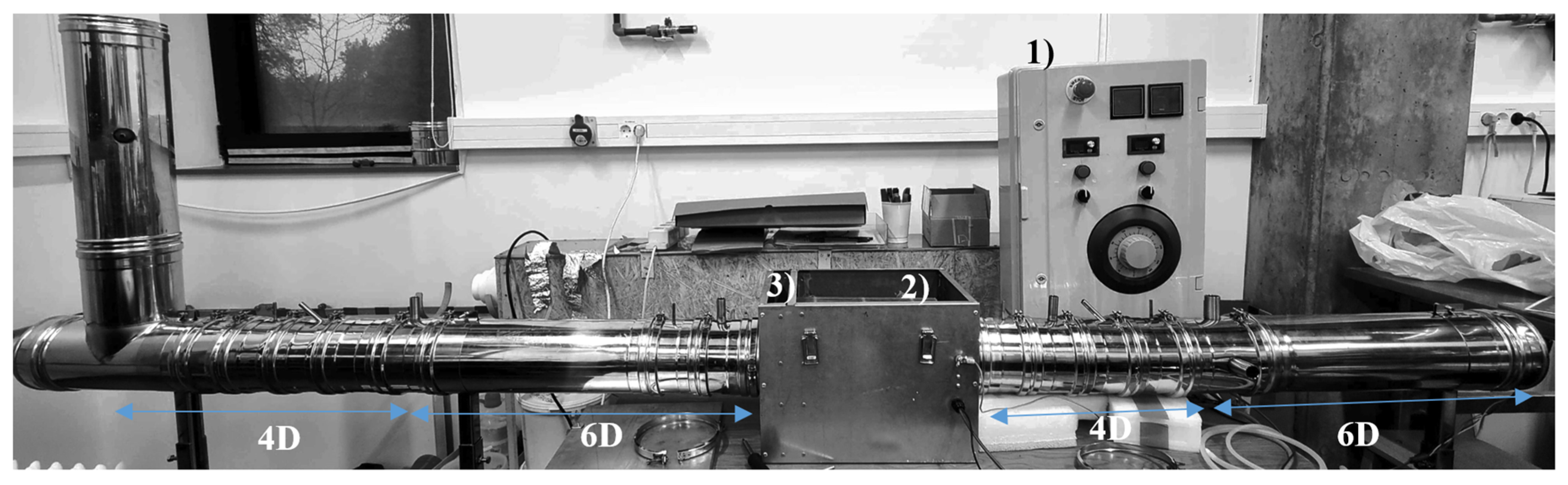
Figure 2.
Principal scheme of the research bench a) and a principal scheme of inlet cross-section view where gas flow rate was measured b), A-E test points in the inlet duct, A1-E1 test points in the outlet duct.
Figure 2.
Principal scheme of the research bench a) and a principal scheme of inlet cross-section view where gas flow rate was measured b), A-E test points in the inlet duct, A1-E1 test points in the outlet duct.
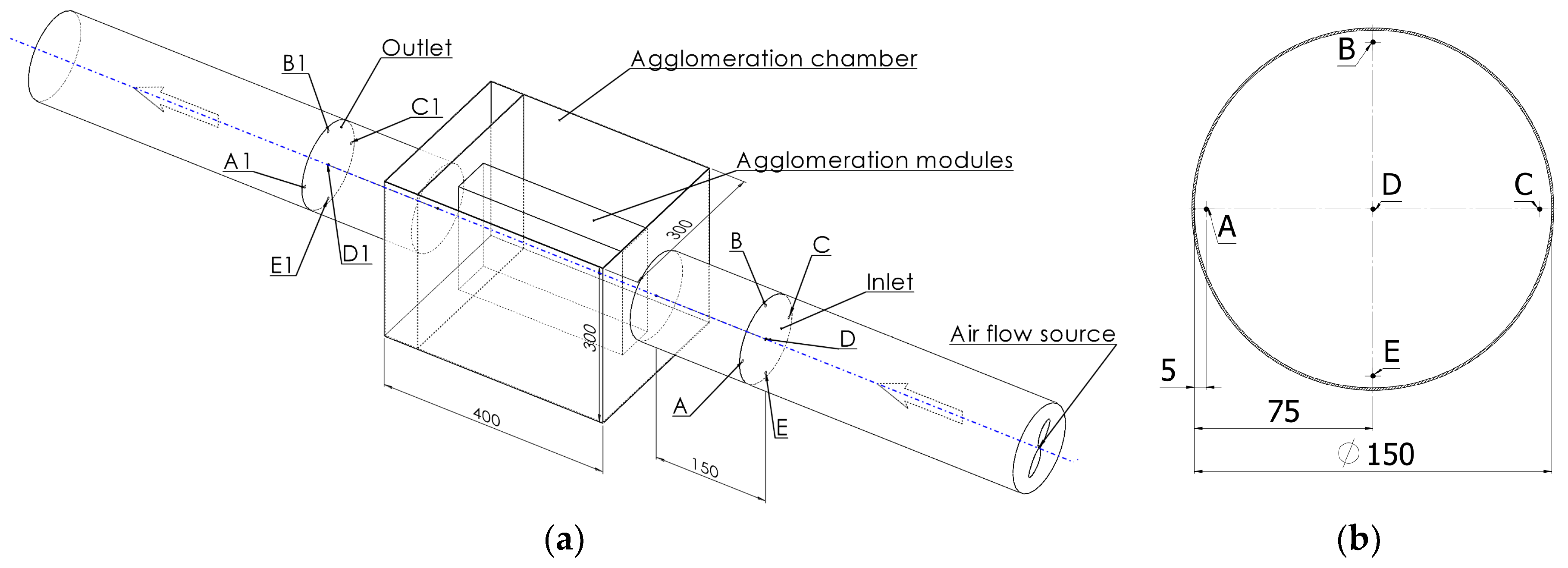
Figure 3.
Available measuring planes (a) and points for gas velocity measurements (b) and four probes to measure the gas velocity in the agglomeration chamber (c).
Figure 3.
Available measuring planes (a) and points for gas velocity measurements (b) and four probes to measure the gas velocity in the agglomeration chamber (c).
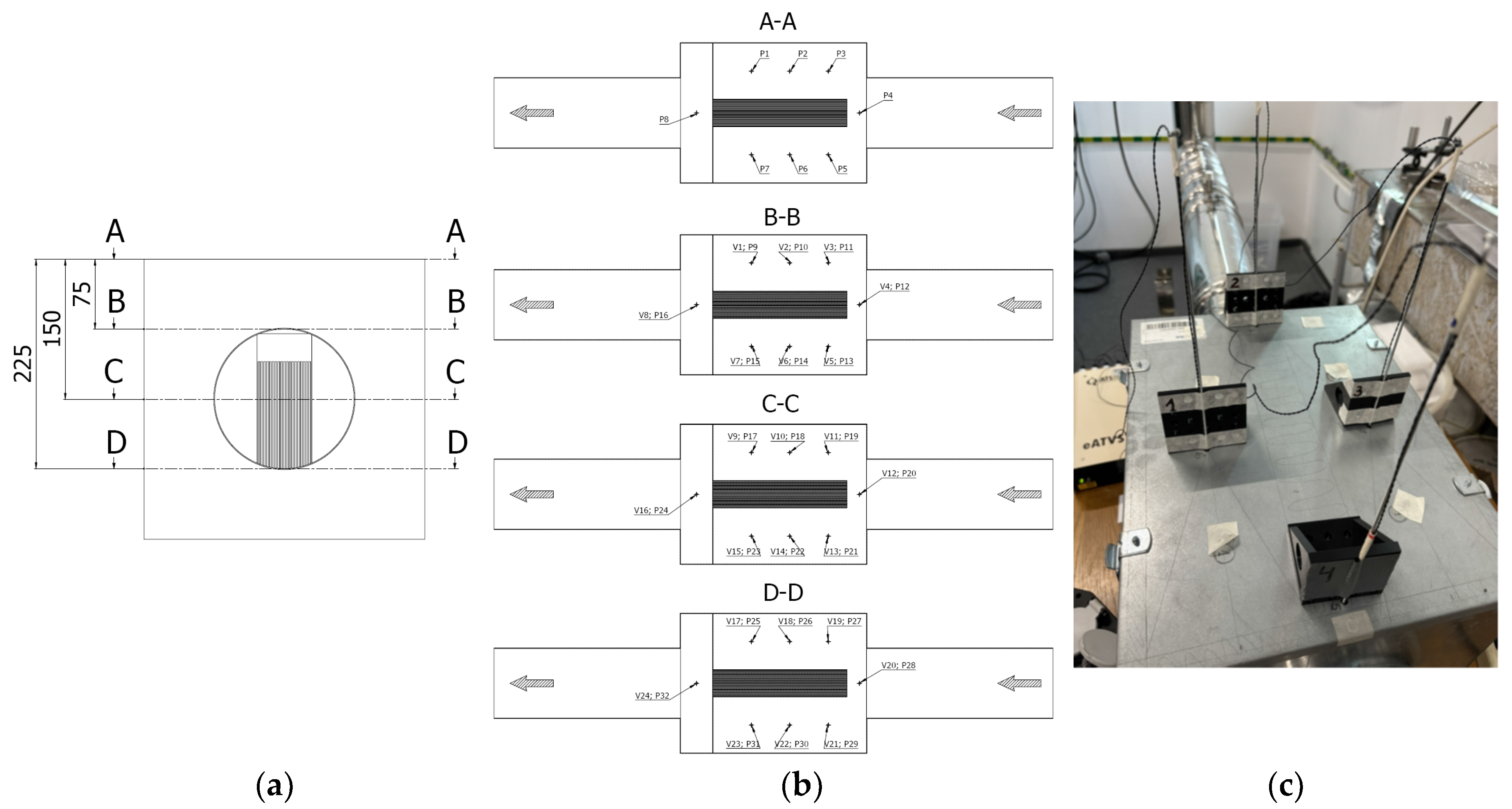
Figure 4.
The distribution of the gas velocity at the inlet at the points of the cross-sectional periphery is presented as a scatter diagram relative to the axial velocity at 50% of the nominal flow.
Figure 4.
The distribution of the gas velocity at the inlet at the points of the cross-sectional periphery is presented as a scatter diagram relative to the axial velocity at 50% of the nominal flow.
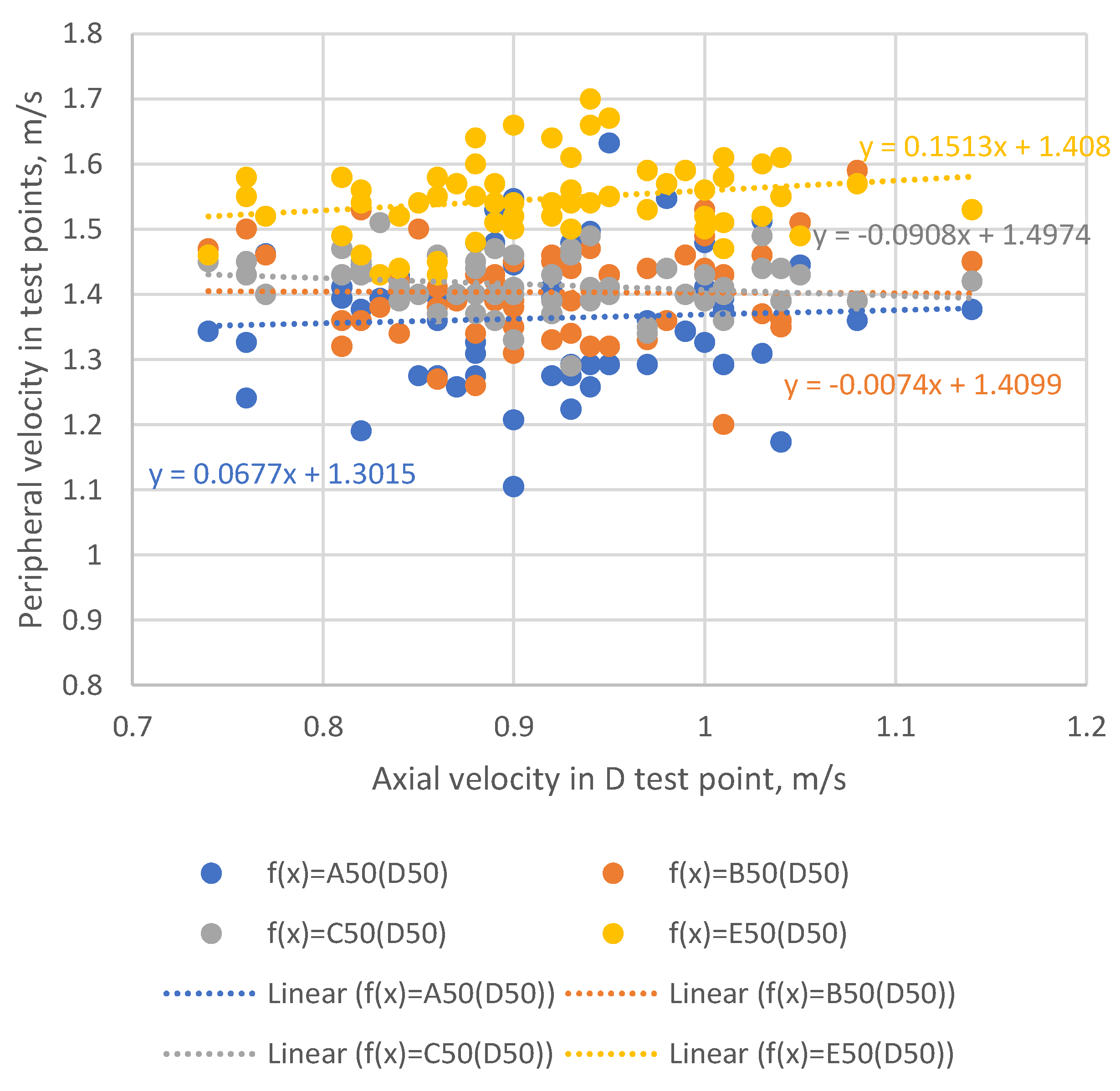
Figure 5.
The distribution of the gas velocity at the outlet at the points of the cross-sectional periphery is presented as a scatter diagram relative to the axial velocity at 50% of the nominal flow.
Figure 5.
The distribution of the gas velocity at the outlet at the points of the cross-sectional periphery is presented as a scatter diagram relative to the axial velocity at 50% of the nominal flow.
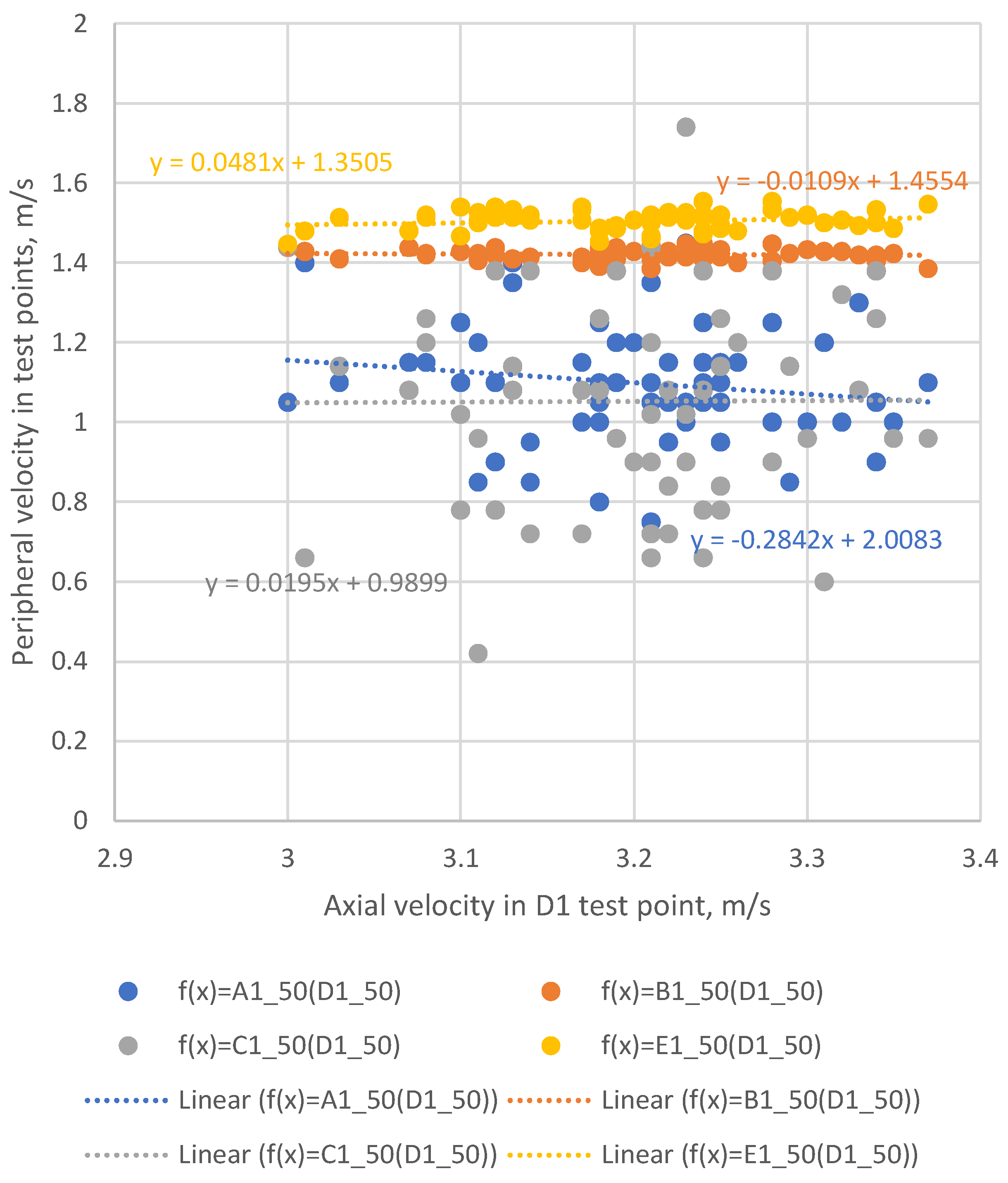
Figure 6.
A dependance of gas flow rate distribution in the center point of inlet (D) and outlet (D1) on the flow rate of a) 10%, b) 50% and c) 100%.
Figure 6.
A dependance of gas flow rate distribution in the center point of inlet (D) and outlet (D1) on the flow rate of a) 10%, b) 50% and c) 100%.
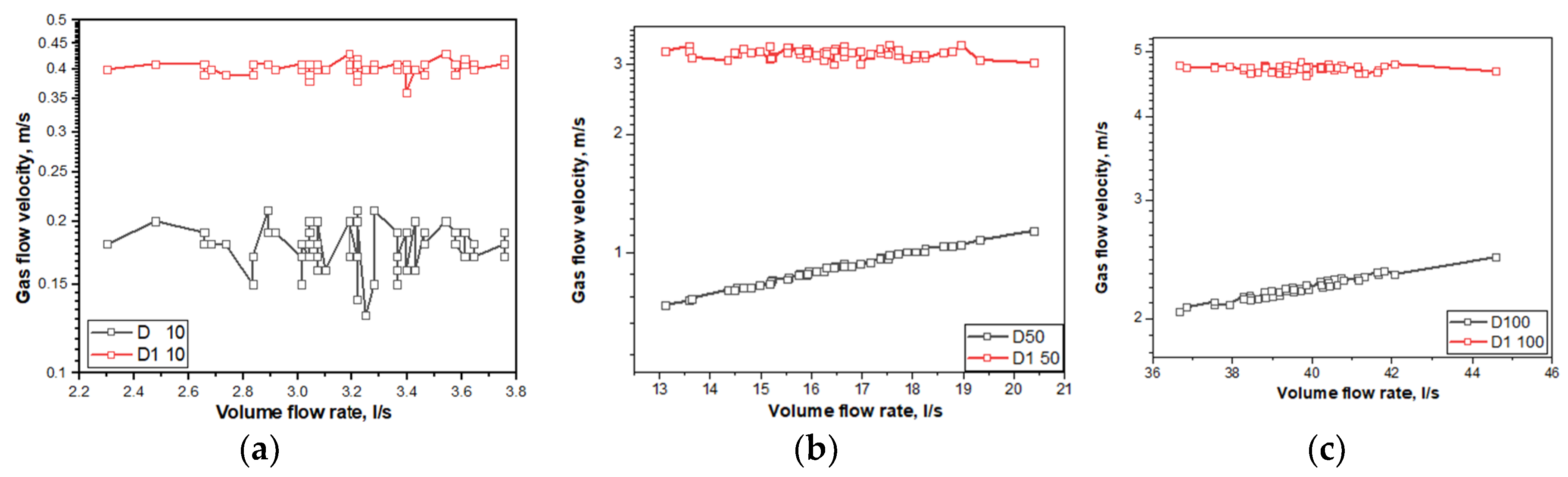
Figure 7.
A dependance of particle number concentration on particle size distribution before and after agglomerator device at nominal voltage of 3.5 kV and current 5 mA.
Figure 7.
A dependance of particle number concentration on particle size distribution before and after agglomerator device at nominal voltage of 3.5 kV and current 5 mA.
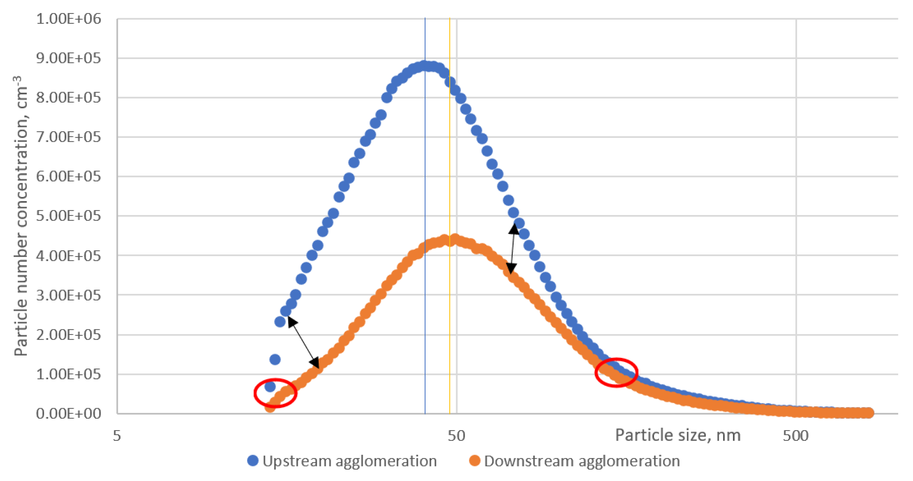
Figure 8.
Velocity distribution along plane a) C−C and plane b) D−D.
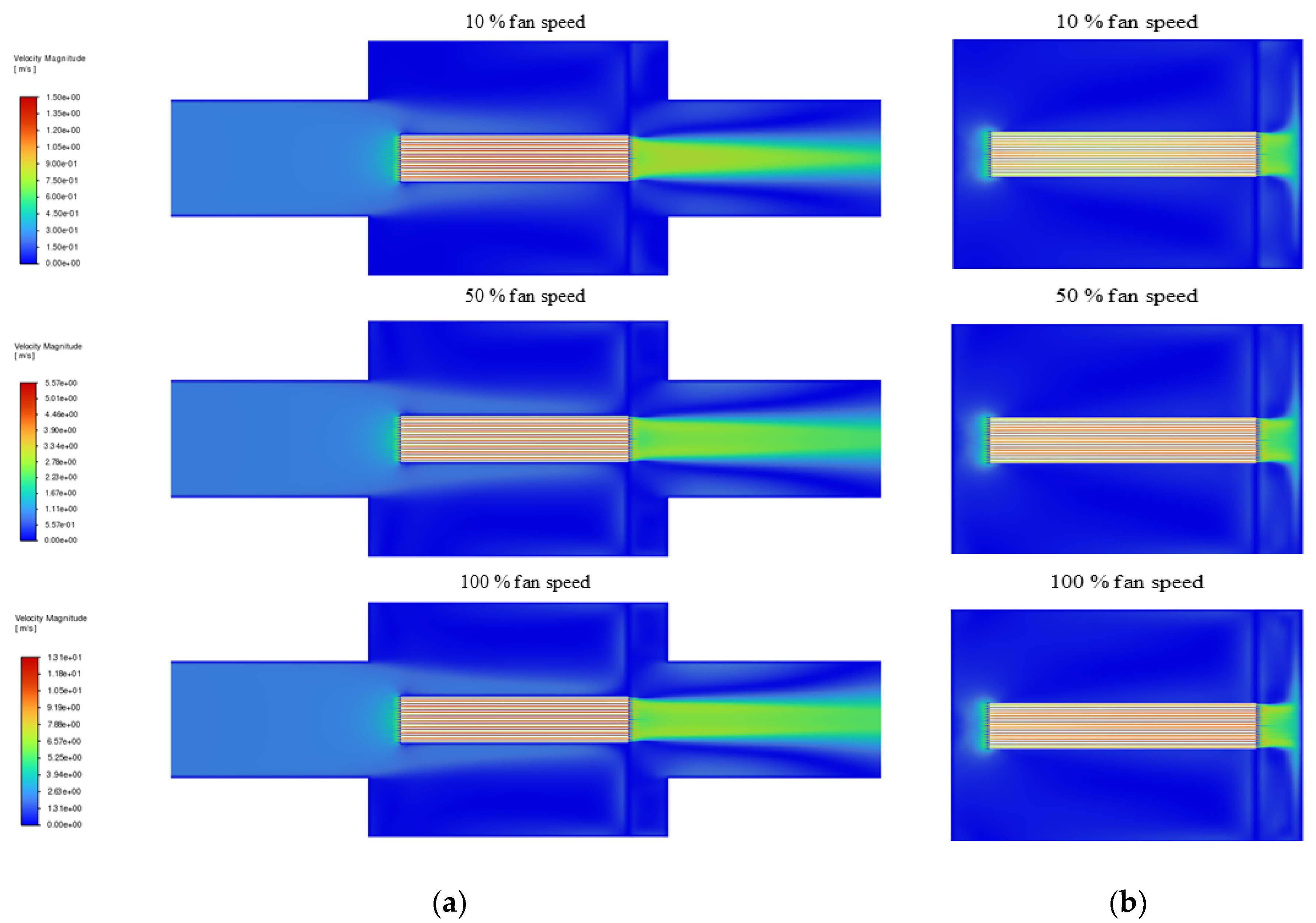
Figure 9.
The resulting velocity vectors along the symmetry plane at different gas flow loads.
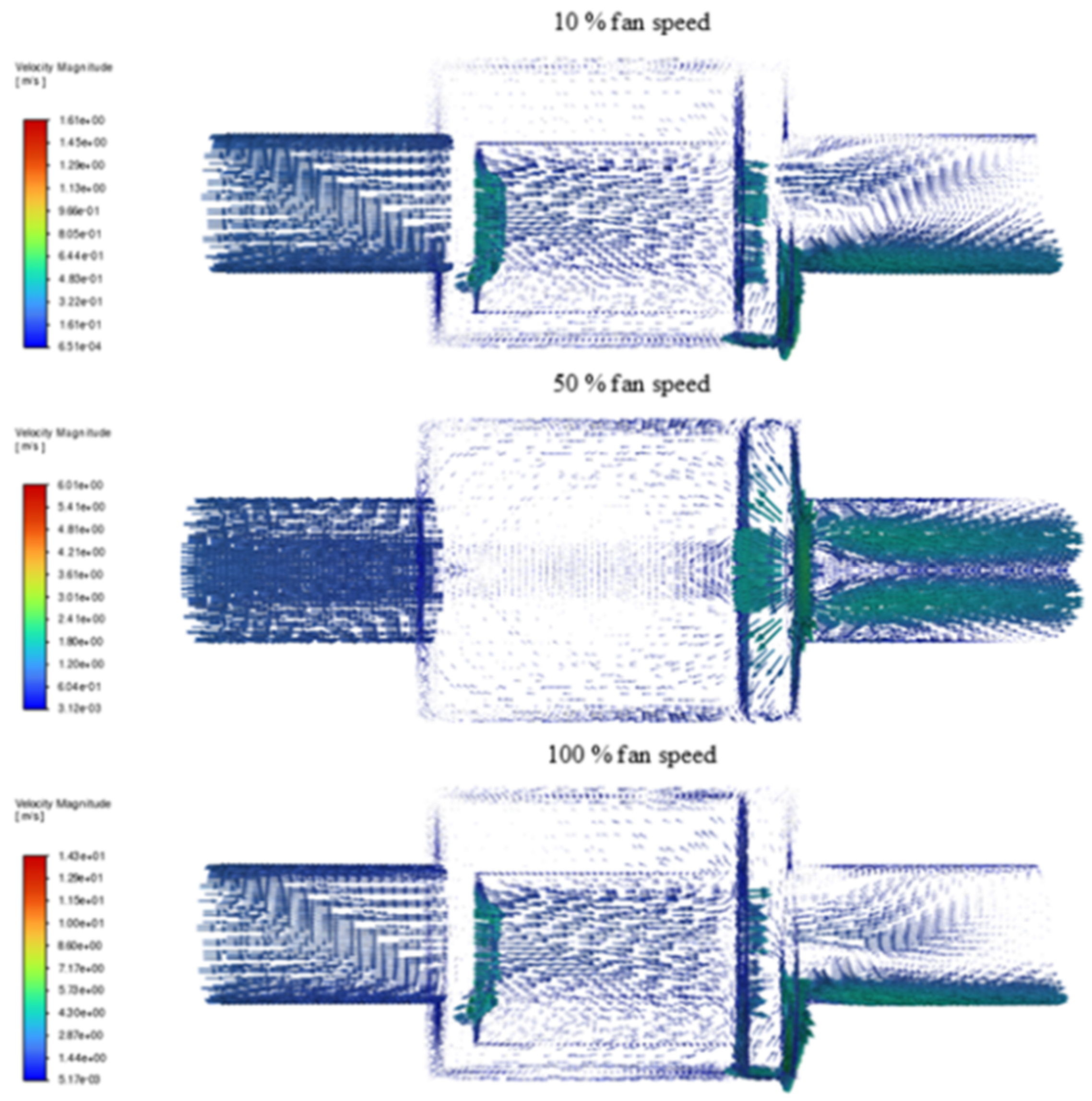
Figure 10.
The resulting particle tracks over 200 time-steps for a particle enters from a fixed location at the inlet.
Figure 10.
The resulting particle tracks over 200 time-steps for a particle enters from a fixed location at the inlet.
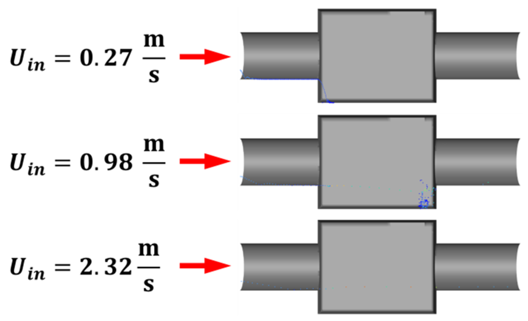
Figure 11.
The resulting particle tracks over 200 time-steps for all particle enters at the inlet at t = 0 s.
Figure 11.
The resulting particle tracks over 200 time-steps for all particle enters at the inlet at t = 0 s.
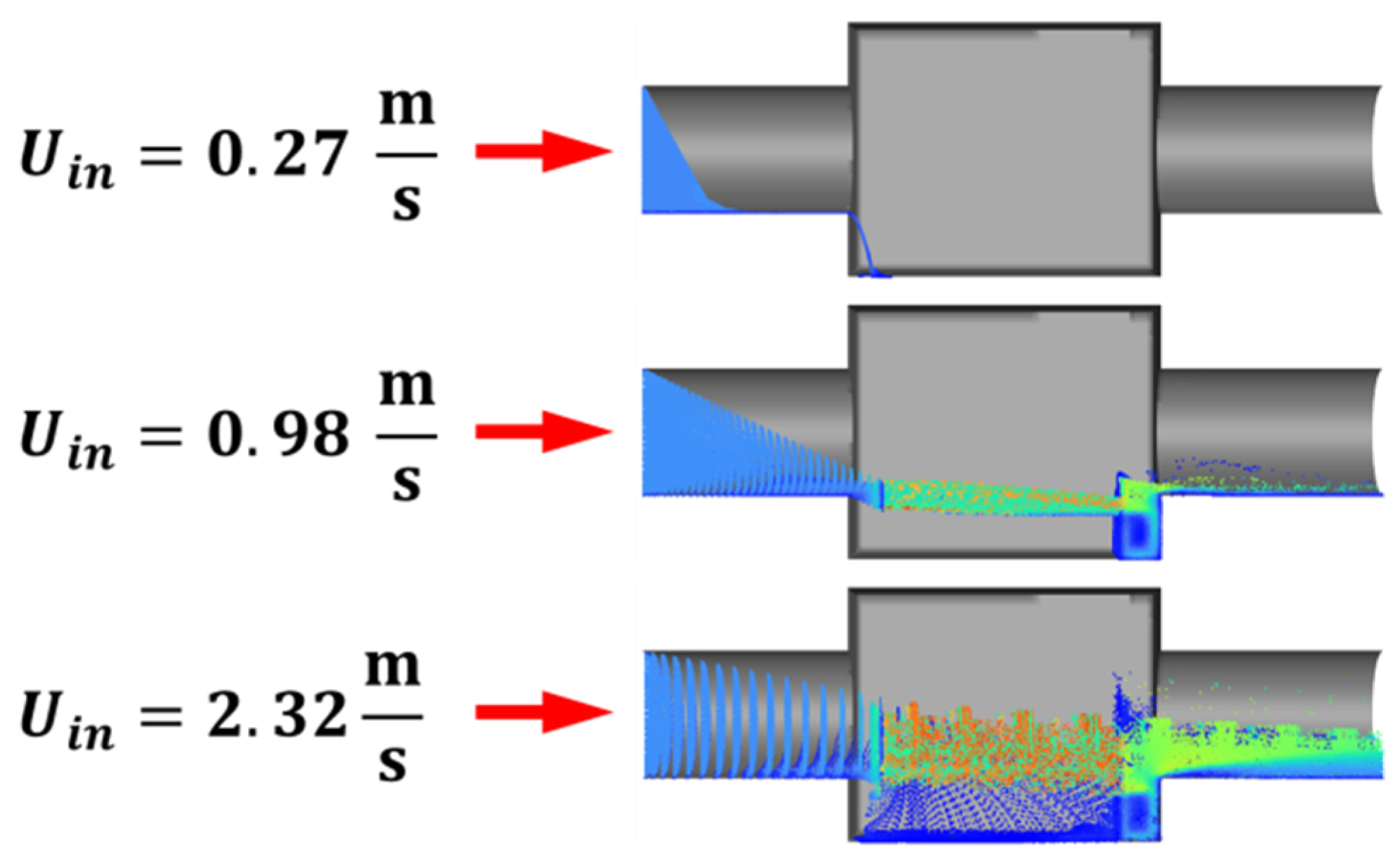
Figure 12.
The velocity distribution in the chamber with carbon particles entering the chamber.
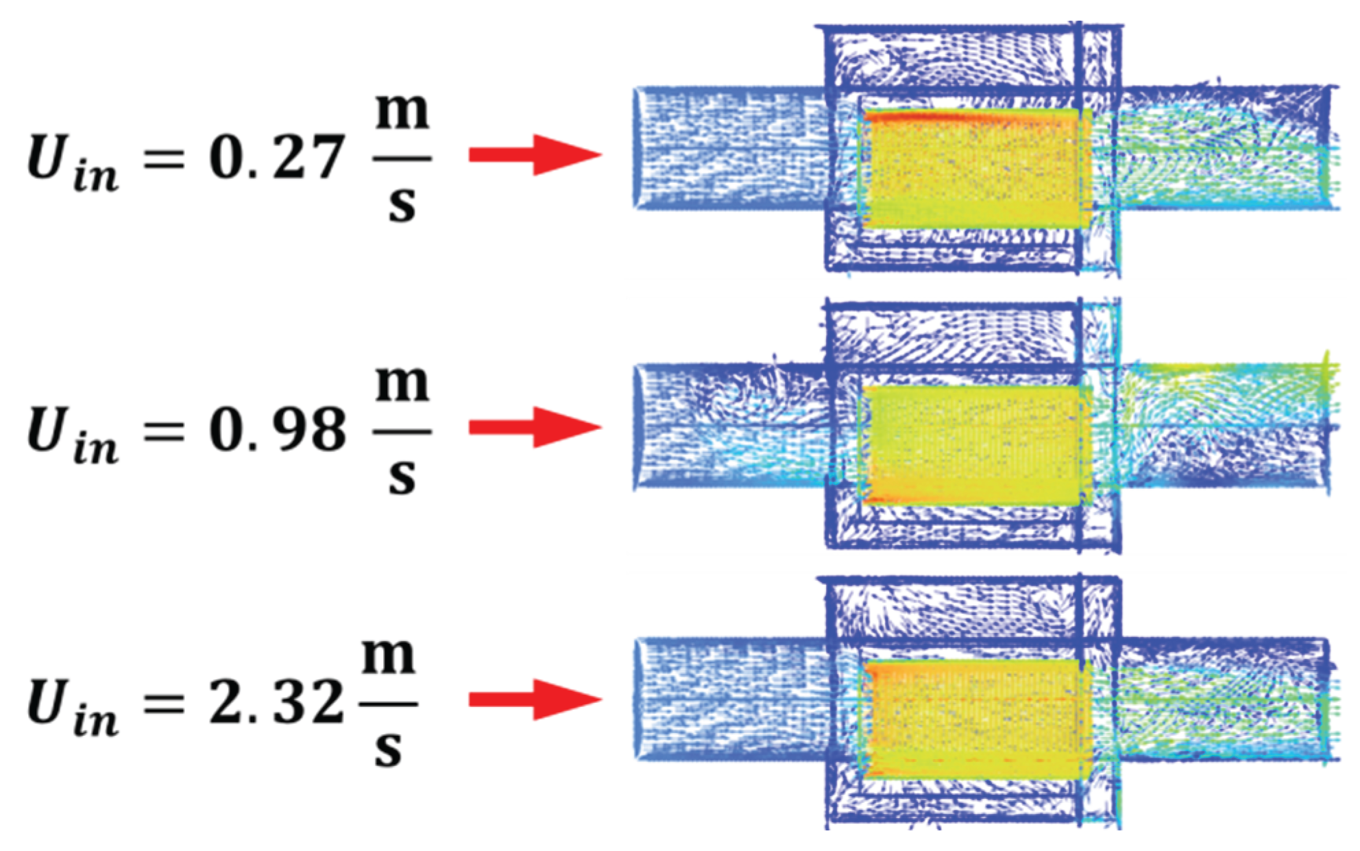

Table 1.
Measuring points, corresponding gas velocity medians at different the gas flow load.
| Location | Measuring point in the inlet duct | Gas flow load (%)) | ||
| 10 | 50 | 100 | ||
| Inlet velocity |
A | 0.27 | 1.65 | 2.79 |
| B | 0.05 | 1.15 | 2.49 | |
| C | 0.17 | 1.60 | 3.25 | |
| D1 | 0.27 | 0.98 | 2.32 | |
| E | 0.12 | 0.99 | 2.47 | |
1The velocity measured on plane D-D are used as the boundary condition at inlet.
Table 2.
A dependance of system resistance and static pressures on the inlet flow amount.
| Gas flow rate, l/s (%) | Aerodynamic resistance, Pa | Static pressure in inlet duct, Pa | Static pressure in outlet duct, Pa |
| 4.65 (10) | 8-9 | 8 | 3 |
| 9.29 (20) | 16 | 16 | 3 |
| 13.94 (30) | 33 | 33 | 3 |
| 18.58 (40) | 49-50 | 50 | 3 |
| 23.23 (50) | 68 | 68 | 3-4 |
| 27.87 (60) | 88 | 88-89 | 4 |
| 32.52 (70) | 109 | 110 | 4-5 |
| 37.16 (80) | 133 | 135-136 | 5 |
| 41.81 (90) | 162 | 165 | 5 |
| 46.45 (100) | 174-175 | 178 | 4-8 |
Table 3.
Series of particle number concentration changes in the upstream and downstream of manipulator depending of nanoparticles size.
Table 3.
Series of particle number concentration changes in the upstream and downstream of manipulator depending of nanoparticles size.
| Particle size, nm | Change of particle number concentration from upstream to downstream | |||
| Average of tests 1 | Average of tests 2 | Average of tests 3 | Main average | |
| 15.1 | -65.5 | -79.9 | -82.0 | -81.7 |
| 20.2 | -61.7 | -73.7 | -73.8 | -72.4 |
| 51.4 | -32.8 | -46.7 | -48.2 | -45.4 |
| 101.8 | -11.3 | -15.0 | -25.4 | -21.3 |
| 151.2 | -12.3 | -6.8 | -17.0 | -16.1 |
| 201.7 | -17.8 | -14.9 | -20.2 | -21.4 |
| 310.6 | -12.1 | -24.2 | -24.5 | -24.3 |
| 399.5 | -18.3 | -29.1 | -24.1 | -25.6 |
| 495.8 | -30.9 | -26.7 | -26.4 | -30.5 |
| 615.3 | -47.3 | -32.2 | -31.8 | -39.8 |
| 710.5 | -34.9 | -29.5 | -28.2 | -32.1 |
| 820.5 | 5.8 | -35.3 | -29.8 | -24.6 |
Table 4.
Comparison of predicted versus measured pressure at selected measurement points on plane C−C in Figure 3.
Table 4.
Comparison of predicted versus measured pressure at selected measurement points on plane C−C in Figure 3.
| Static pressure [Pa] | ||||||
| Gas flow load, % | V23 | V26 | V27 | V28 | V31 | |
| Experiment | 10 | 7 | 7 | 7 | 7 | 0 |
| Simulation | 6.41 | 6.53 | 6.53 | 6.53 | 3.05 | |
| Experiment | 50 | 65 | 67 | 67 | 67 | −1 |
| Simulation | 65.4 | 66.94 | 66.93 | 66.93 | 14 | |
| Experiment | 100 | 167 | 177 | 176 | 176 | −7 |
| Simulation | 222.71 | 231.4 | 231.28 | 231.22 | −76.42 | |
Table 5.
Comparison of predicted versus measured pressure at selected measurement points on plane D−D in Figure 3.
Table 5.
Comparison of predicted versus measured pressure at selected measurement points on plane D−D in Figure 3.
| Static pressure [Pa] | ||||||
| Gas flow load, % | V38 | V41 | V42 | V43 | V46 | |
| Experiment | 10% | 9 | 9 | 9 | 10 | 2 |
| Simulation | 6.43 | 6.53 | 6.53 | 6.53 | 3.07 | |
| Experiment | 50% | 69 | 69 | 70 | 70 | 1 |
| Simulation | 65.52 | 66.93 | 66.93 | 66.93 | 14.36 | |
| Experiment | 100% | 177 | 179 | 179 | 178 | −3 |
| Simulation | 223.22 | 231.27 | 231.26 | 231.22 | −74.56 | |
Disclaimer/Publisher’s Note: The statements, opinions and data contained in all publications are solely those of the individual author(s) and contributor(s) and not of MDPI and/or the editor(s). MDPI and/or the editor(s) disclaim responsibility for any injury to people or property resulting from any ideas, methods, instructions or products referred to in the content. |
© 2026 by the authors. Licensee MDPI, Basel, Switzerland. This article is an open access article distributed under the terms and conditions of the Creative Commons Attribution (CC BY) license (http://creativecommons.org/licenses/by/4.0/).
Copyright: This open access article is published under a Creative Commons CC BY 4.0 license, which permit the free download, distribution, and reuse, provided that the author and preprint are cited in any reuse.


