
Submitted:
26 January 2026
Posted:
27 January 2026
You are already at the latest version
Abstract
This study investigates the extent to which demand-load prediction and adaptive load control in photovoltaic heating systems depend on computationally intensive artificial neural network (ANN) models. We propose a load-prediction algorithm and a corresponding control strategy designed to streamline the computational workflow and reduce resource requirements. By optimizing the algorithmic structure, the proposed method reduces the computational burden during operation while preserving predictive accuracy. The streamlined workflow enables efficient load prediction and adaptive control in real-time operation. Compared with conventional ANN models, the proposed method achieves an overall (all-interval) mean deviation of −0.2%. Moreover, the proposed adaptive load-control strategy requires only 3.9% of the computational resources needed by conventional approaches. The method rapidly reallocates computational resources in response to changes in real-time input data, thereby minimizing redundant computations. Overall, the results indicate that the proposed algorithm substantially reduces computational complexity while maintaining high predictive accuracy. This approach offers an effective alternative to traditional ANN-based methods and facilitates the practical deployment of photovoltaic heating systems.
Keywords:
adaptive load
; photovoltaic heating system
; artificial neural network
; system modeling
; optimization of methodological models
1. Introduction
With the growing global emphasis on renewable energy, photovoltaic heating systems—integrating solar-to-electric conversion with thermal energy delivery—have emerged as a major research focus for improving building energy efficiency and enabling clean heating. By aligning photovoltaic power generation with thermal demand, these systems can reduce reliance on fossil fuels and improve overall energy-utilization efficiency [1]. However, optimizing system performance remains challenging because it requires accurate dynamic load prediction and coordinated real-time responses. These requirements jointly shape the trade-off between conversion efficiency and operating cost [2]. Numerous maximum power point tracking (MPPT) methods have been developed for photovoltaic (PV) systems [3], including particle swarm optimization (PSO), Lyapunov control schemes (LCS), incremental conductance (IC), fuzzy logic control (FLC), artificial neural networks (ANN), ripple correlation control (RCC), perturb-and-observe (P&O), and Fisher discriminant dictionary learning (FDDL) [4,5,6,7,8,9,10,11,12,13]. These approaches are typically evaluated under varying irradiance and shading conditions, often with additional environmental factors taken into account. Prior studies indicate that ANN-based MPPT can harvest more electrical energy from PV arrays than many alternative methods under diverse irradiance profiles [14,15]. Accordingly, load prediction and control in photovoltaic heating systems often rely on complex ANN-based models trained on large historical datasets to capture nonlinear load dynamics and achieve high predictive accuracy [16,17]. Nevertheless, multi-layer parameter optimization and iterative computations can impose substantial computational costs and increase response latency in practical implementations. In distributed deployments (e.g., remote areas or small communities), these requirements may exceed local hardware capabilities, thereby limiting adoption. Moreover, training and maintaining ANN models typically require long-term, high-quality datasets, which can be difficult to obtain and maintain due to data-collection costs and nonstationary environmental conditions. Although MPPT primarily maximizes electrical power extraction from a PV array, its benefit in photovoltaic heating systems is ultimately realized through downstream load matching and control. This is because the operating point imposed by the thermal load (or the power-electronic interface) couples the electrical maximum power point (MPP) to instantaneous heating demand and overall system efficiency.
To address these limitations, this paper proposes a load-prediction algorithm and an adaptive load-control model that retain key advantages of ANN-based approaches while substantially reducing computational complexity and resource requirements. By optimizing model structure and parameter selection, the proposed method avoids the multi-layer iterations and complex optimization procedures typical of conventional ANN implementations, thereby reducing computational load while maintaining reliable predictive performance. The proposed method is evaluated by comparing annual cumulative output power with that of a conventional ANN-based adaptive load-prediction model.
In addition, we compare the data-call volume of the two control models to quantify the computational savings achieved by the simplified controller. This study makes two primary contributions. First, the simplified design alleviates the computational bottleneck of conventional methods and improves the feasibility of lightweight deployment in photovoltaic heating systems. Second, the method’s stability and accuracy under long-term operation are validated, providing empirical support for engineering applications. Beyond photovoltaic heating, the proposed low-complexity framework may be applicable to other distributed energy-management tasks, such as wind-power load matching and microgrid scheduling. From a societal perspective, reducing computational and operational costs can facilitate clean-energy deployment in resource-constrained settings and support progress toward dual-carbon targets and improved energy equity.
2. Construction of the Load Prediction Model for the Photovoltaic Heating System
2.1. Modeling and Simulation of Irradiance and Ambient Temperature
Using TRNSYS, we modeled the annual solar irradiance incident on a surface tilted at 39° and the corresponding ambient-temperature variations [18]. The model generated hourly irradiance data for periods in which irradiance exceeded 100 W/m² (Figure 1). As shown in Figure 1, the plane-of-array (tilted-surface) irradiance ranges from 100.6 to 1287.3 W/m², and the corresponding ambient temperature varies from −22.2 to 33.3 °C. Hourly samples with irradiance in the 100–200 W/m² range were excluded from the binning analysis and subsequent model construction; they were retained only for completeness in the initial hourly irradiance dataset (Figure 1). For subsequent analysis, irradiance values exceeding 200 W/m² were classified into five 200 W/m² intervals. To avoid ambiguity at bin boundaries, the irradiance intervals were defined as half-open ranges: [200, 400), [400, 600), [600, 800), and [800, 1000), with the final interval defined as [1000, ∞) W/m² (up to the observed maximum of 1287.3 W/m²). Accordingly, boundary values (e.g., 400 W/m²) were assigned to the upper interval [19,20]. The annual cumulative irradiance fractions within these intervals were 12.0%, 19.7%, 25.2%, 31.6%, and 11.6%, respectively (Figure 2). We also computed the annual mean irradiance and the corresponding mean ambient temperature for each interval (Figure 3). These results were used as inputs to the subsequent Simulink-based simulations.
2.2. Establishment of the Simplified Load Solution Model for the Photovoltaic Heating System
The Ulica Solar UL-330M-60 module was used as the PV module model, and its key parameters are summarized in Table 1. The module has a rated maximum power of Pmax=330W at the maximum power point, with Vmpp =33.5V and Impp =9.85A. The datasheet also reports the open-circuit voltage Voc, short-circuit current Isc, and the temperature coefficients for voltage and current. These ratings are specified under Standard Test Conditions (STC), i.e., an irradiance of 1000 W/m² and a cell temperature of 25 °C. Multiple PV modules were electrically interconnected to form an array. Simulations were performed for an array configuration of Ns ×Np = 2×1, where Ns and Np denote the numbers of series- and parallel-connected modules, respectively. This array configuration was used to evaluate the computational model and its design parameters.
2.2.1. Maximum Output Power and Internal Resistance Calculation
Based on an array comprising two PV modules connected in series (Table 1), we implemented a no-load maximum power point (MPP) model in Simulink (Figure 4). In this model, irradiance Sand cell temperature T were used as inputs. These inputs were set to the annual mean irradiance and the corresponding annual mean cell temperature for the five irradiance intervals defined above.
Prior studies indicate that the temperature difference between ambient air and PV cell temperature typically ranges from 20 to 30 °C [21,22]. Here, we adopted a conservative offset of 30 °C; therefore, the cell temperature was set to the annual mean ambient temperature plus 30 °C. Based on the results in Section 2.1, the annual mean irradiance S for the five intervals was 1053.2, 898.6, 699.8, 497.4, and 302.4 W/m², respectively. The corresponding annual mean cell temperatures T were 43.5, 41.2, 39.0, 40.9, and 41.8 °C. For each interval, the model outputs the maximum power and the corresponding MPP voltage under the specified Sand T conditions. Using Ohm’s law, we calculated the equivalent internal resistance at each MPP as 6.1, 7.1, 9.3, 13.2, and 21.3 Ω (Figure 5).
Based on the maximum power transfer theorem, we implemented a loaded MPP model in Simulink (Figure 6). The resulting maximum output powers after load connection were 628.2, 542.3, 429.2, 302.2, and 180.7 W across the five irradiance intervals (Figure 7).
By comparing the loaded model (Figure 6) with the no-load model (Figure 4), we obtained relative power errors of 2.9%, 3.1%, 2.9%, 2.8%, and 3.0% across the five intervals (Figure 8). This error analysis supports the reliability of the proposed modeling approach and provides a basis for subsequent calculations of annual cumulative power output.
2.3. Construction of the Adaptive Load Power Prediction Model for the Photovoltaic Heating System
Prior studies indicate that artificial neural networks (ANNs) are among the most effective approaches for modeling the power characteristics relevant to maximum power point tracking (MPPT) in photovoltaic systems. To evaluate the predictive performance of the simplified load model in Section 2.2, we developed an ANN-based adaptive load–power prediction model (Figure 9). The model comprises three modules: a data-input interface, a trained ANN model, and an output interface. The workflow is summarized as follows. The input interface provides irradiance and cell temperature to the trained ANN model. The trained ANN then estimates the maximum output power at the corresponding operating point via inference. During inference, the ANN performs a forward-propagation pass using stored network weights (i.e., weight retrieval followed by feedforward evaluation) to estimate the output; no online iterative optimization or parameter updating is performed. Finally, the output interface returns the predicted value.
Constructing the trained ANN model is a key step in the proposed predictive framework. The training dataset comprises maximum output power values corresponding to discrete irradiance levels and cell temperatures. Based on the meteorological data in Figure 1, irradiance values above 200 W/m² were discretized into 10 bins with a 100 W/m² step over 250–1150 W/m², and the midpoint of each bin was used as the representative value. Ambient temperature was discretized into 13 bins with a 5 °C step over −30 to 30 °C. As defined in Section 2.2.1, cell temperature was set to ambient temperature plus 30 °C, yielding a range of 0–60 °C. Using the above discretization scheme and the no-load Simulink MPP model (Figure 4), we systematically computed the maximum output power and equivalent internal resistance for each irradiance bin across all temperature bins. Figure 10 illustrates the maximum output power across the 13 cell-temperature bins (0–60 °C) at an irradiance of 1150 W/m².
Maximum power outputs under the remaining irradiance conditions were computed using the same procedure. Using the complete set of simulation results, we constructed the trained ANN model with 10×13=130 nodes (Figure 11). These 130 nodes correspond to the 10 irradiance bins and 13 temperature bins (i.e., 10×13 combinations).
3. Results and Discussion
3.1. Output Power Calculation of the Simplified Model
Following the approach described in Section 2, the simplified model partitions irradiance into five intervals, each associated with a corresponding cell temperature. Using Simulink, five equivalent internal resistances r1-r5 were calculated as 6.1, 7.1, 9.3, 13.2, and 21.3 Ω, respectively.
The equivalent internal resistance at the maximum power point (MPP) was computed as follows:
where Vmpp and Impp denote the voltage and current at the maximum power point, respectively.
According to the maximum power transfer theorem, maximum power is delivered when the load resistance equals the corresponding internal resistance (i.e., RL1-RL5 = r1-r5).
We propose an adaptive-load photovoltaic direct-heating system; its operating principle is shown in Figure 12. The system dynamically selects among five load resistors (RL1-RL5) based on the real-time measured plane-of-array irradiance S. Specifically, when S∈ [200,400) W/m², contactor KM5 closes to connect RL5; otherwise, KM5 remains open. Similarly, for S∈[400,600), [600,800), [800,1000), and [1000,1200] W/m², contactors KM4–KM1 close, respectively, to connect RL4, RL3, RL2 and RL1, thereby supplying power for water heating. To prevent parallel activation of multiple loads, contactors KM1–KM5 operate in a mutually exclusive (interlocked) mode such that only one contactor can be closed at any time, corresponding to the active irradiance interval. To avoid ambiguity at bin boundaries, the irradiance intervals are defined as half-open ranges: [200, 400), [400, 600), [600, 800), and [800, 1000), with the final interval defined as [1000,1200] W/m². Accordingly, a boundary value (e.g., 400 W/m²) is assigned to the upper interval, whereas 1200 W/m² is included in the final interval. The contactor coils are powered by an external AC supply.
3.2. Cumulative Output Power Calculation Using the Artificial Neural Network
Using the hourly plane-of-array irradiance from Figure 1, together with the cumulative irradiance fractions, mean irradiance values, and interval power outputs from Figure 2 and Figure 3, and 7, the system computes the cumulative output power for each interval (Figure 13). Using the same procedure, the hourly plane-of-array irradiance from Figure 1 was fed into the ANN-based output-power prediction model (Figure 9). The load was assumed to respond dynamically to the input conditions and to utilize all generated power (i.e., no curtailment). The simulation outputs were post-processed to obtain the ANN-predicted cumulative output power for each interval (Figure 13).
Comparison of the two models across the five intervals shows that the deviation between the ANN model and the simplified model ranges from −0.9% to 0.1%. The overall (all-interval) mean deviation is −0.2%. Given the small deviation, the simplified model achieves accuracy comparable to the ANN baseline and is therefore suitable for practical engineering applications.
The deviation was quantified as the relative error with respect to the ANN baseline. For each interval i, the relative error was defined as follows:
Where Psimp and PANN denote the cumulative output power predicted by the simplified model and the ANN model, respectively.
The overall (all-interval) mean deviation was computed as an irradiance-fraction–weighted mean of the interval-wise relative errors, defined as follows:
Where wi denotes the annual irradiance fraction (or time-share) associated with interval i, and δi is the corresponding relative error.
3.3. Comparison of Data Requirements for Control Output of Two Models
To reduce the computational burden of maximum output-power prediction, we simulated local meteorological conditions and extracted hourly irradiance and temperature data. The annual irradiance time series was grouped into five intervals with a 200 W/m² step, and the annual mean irradiance and corresponding mean temperature were calculated for each interval. A no-load Simulink model was established to compute the maximum output power and the equivalent internal resistance at the maximum power point (MPP) for each of the five operating points. A loaded Simulink model was then built to compute the maximum output power and the equivalent internal resistance at the MPP after load connection for each of the five operating points. Based on these results, we implemented a simplified ANN-based control model (Figure 14) for adaptive load matching.
The controller uses a single input—plane-of-array irradiance—and includes five ANN nodes. For a given irradiance input, the controller identifies the corresponding interval, selects the associated node value, and switches in the matched load to initiate water heating. Owing to its low computational demand, the controller enables rapid response. For the ANN-based maximum-power prediction model, we used the same meteorological simulations to obtain hourly irradiance and temperature data. The annual irradiance time series was discretized into 10 intervals with a 100 W/m² step, and ambient temperature was discretized into 13 intervals with a 5 °C step.
A no-load Simulink model was used to compute the maximum output power and the equivalent internal resistance at the MPP for all 130 operating points. A loaded Simulink model was further used to compute the maximum output power and the equivalent internal resistance at the MPP after load connection for the same 130 operating points. Based on these results, adaptive load matching was performed using the ANN-based controller (Figure 15).
The controller uses two inputs—plane-of-array irradiance and PV cell temperature—and contains 130 ANN nodes. Given irradiance and cell-temperature inputs, the controller determines the corresponding intervals, retrieves the associated node value from the 130 candidates, and switches in the matched load to initiate water heating. Consequently, this approach requires substantially greater computational resources and incurs higher implementation cost.
4. Conclusion
This study systematically compares conventional ANN-based prediction and control models with simplified counterparts using TRNSYS-generated meteorological data for training and validation. The main findings are summarized as follows:
(1) For annual cumulative output power, the absolute deviation between the conventional and simplified prediction models ranges from 0.1% to 0.9%, and the overall (all-interval) mean deviation is −0.2%. This narrow deviation range indicates that the simplified prediction model achieves accuracy comparable to the conventional model.
(2) Regarding data-call efficiency, the conventional controller uses 130 nodes, whereas the simplified controller uses five, corresponding to 3.85% of the conventional model’s node count. This reduction indicates that the simplified controller can substantially decrease computational demand and associated hardware cost. Consequently, the simplified controller provides a practical alternative to computationally intensive ANN-based approaches by offering a favorable trade-off between performance and cost.
Author Contributions
For research articles with several authors, a short paragraph specifying their individual contributions must be provided. The following statements should be used “Conceptualization, S.M. Xu.; methodology, S.M. Xu.; software, S.M. Xu.; validation, Y.X. Wang, S.L. An.; formal analysis, S.M. Xu.; investigation, Y.X. Wang; resources, Y.X. Wang; data curation, S.M. Xu.; writing—original draft preparation, S.M. Xu.; writing—review and editing, S.L. An.; visualization, S.M. Xu.; project administration, Y.X. Wang; funding acquisition, Y.X. Wang. All authors have read and agreed to the published version of the manuscript.”
Funding
This research was funded by Inner Mongolia Applied Technology Research & Development Foundation, grant number 2023JBGS0012.
Data Availability Statement
The datasets generated during this study are fully available within the article and supplementary materials.
Acknowledgments
The authors would like to acknowledge the support of Inner Mongolia Applied Technology Research & Development Foundation (2023JBGS0012) for this work.
Conflicts of Interest
The authors declare that they have no known competing financial interests or personal relationships that could have appeared to influence the work reported in this paper.
Abbreviations
The following abbreviations are used in this manuscript:
| MPP | Maximum power point; |
| ANN | Artificial neural network; |
| VOC | The open-circuit voltage of PV module, V; |
| ISC | The short-circuit current, A; |
| Vmpp | The optimal voltage at maximum power point, V; |
| Impp | The optimal current at maximum power point, A; |
| RL | Load resistance |
References
- Samykano, M. Hybrid photovoltaic thermal systems: present and future feasibilities for industrial and building applications[J]. Buildings 2023, 13(8), 1950. [Google Scholar] [CrossRef]
- A. Gaga, F. Errahimi, N. Es-Sbai, Design and Implementation of MPPT Solar System Based on the Enhanced P&O lgorithm Using Labview. In International Renewable and Sustainable Energy Conference (IRSEC); 2020; pp. 203–208. [CrossRef]
- Katche, M L; Makokha, A B; Zachary, S O; et al. A comprehensive review of maximum power point tracking (mppt) techniques used in solar pv systems[J]. Energies 2023, 16(5), 2206. [Google Scholar] [CrossRef]
- Shami, T M; El-Saleh, A A; Alswaitti, M; et al. Particle swarm optimization: A comprehensive survey[J]. Ieee Access 2022, 10, 10031–10061. [Google Scholar] [CrossRef]
- Baghaee, H R; Mirsalim, M; Gharehpetian, G B; et al. A decentralized power management and sliding mode control strategy for hybrid AC/DC microgrids including renewable energy resources[J]. In IEEE transactions on industrial informatics; 2017. [Google Scholar] [CrossRef]
- Sun, C; Ling, J; Wang, J. Research on a novel and improved incremental conductance method[J]. Scientific Reports 2022, 12(1), 15700. [Google Scholar] [CrossRef] [PubMed]
- Hannan, M A; Ghani, Z A B D; Hoque, M M; et al. Fuzzy logic inverter controller in photovoltaic applications: Issues and recommendations[J]. Ieee Access 2019, 7, 24934–24955. [Google Scholar] [CrossRef]
- Qamar, R; Zardari, B A. Artificial neural networks: An overview[J]. Mesopotamian Journal of Computer Science 2023, 2023, 124–133. [Google Scholar] [CrossRef] [PubMed]
- Wu, Yc.; Feng, Jw. Development and Application of Artificial Neural Network. Wireless Pers Commun 2018, 102, 1645–1656. [Google Scholar] [CrossRef]
- Walczak, S. Artificial neural networks[M]//Advanced methodologies and technologies in artificial intelligence, computer simulation, and human-computer interaction; IGI Global Scientific Publishing, 2019; pp. 40–53. [Google Scholar] [CrossRef]
- Ibrahim, A A; Caldognetto, T; Biadene, D; et al. Multidimensional ripple correlation technique for optimal operation of triple-active-bridge converters[J]. IEEE Transactions on Industrial Electronics 2022, 70(8), 8032–8041. [Google Scholar] [CrossRef]
- Ahmad, M E; Numan, A H; Mahmood, D Y. A comparative study of perturb and observe (P&O) and incremental conductance (INC) PV MPPT techniques at different radiation and temperature conditions[J]. Eng. Technol. J 2022, 40(2), 376–385. [Google Scholar] [CrossRef]
- Zhou, L; Wang, S; Zhao, Z; et al. Low-dimensional multi-scale Fisher discriminant dictionary learning for intelligent gear-fault diagnosis[J]. Measurement Science and Technology 2021, 32(8), 084001. [Google Scholar] [CrossRef]
- Saxena, A; Kumar, R; Amir, M; et al. Maximum power extraction from solar PV systems using intelligent based soft computing strategies: A critical review and comprehensive performance analysis[J]. Heliyon 2024, 10(2). [Google Scholar] [CrossRef] [PubMed]
- Hussain, M T; Sarwar, A; Tariq, M; et al. An evaluation of ANN algorithm performance for MPPT energy harvesting in solar PV systems[J]. Sustainability 2023, 15(14), 11144. [Google Scholar] [CrossRef]
- Rao, S N V B; Yellapragada, V P K; Padma, K; et al. Day-ahead load demand forecasting in urban community cluster microgrids using machine learning methods[J]. Energies 2022, 15(17), 6124. [Google Scholar] [CrossRef]
- Amit, M.; Prajapat, AK.; Refat, S.S. Dynamic performance evaluation of grid-connected hybrid renewable energy-based power generation for stability andpower quality enhancement in smart grid. Front. Energy Res. 2022, 10, 861282. [Google Scholar] [CrossRef]
- Redpath, D; Paneri, A; Singh, H; et al. Design of a building-scale space solar cooling system using TRNSYS[J]. Sustainability 2022, 14(18), 11549. [Google Scholar] [CrossRef]
- Fragkos, K; Charalampous, G; Fountoulakis, I; et al. Next-day solar irradiance forecasting: A preliminary study in Limassol[C]//2024 3rd International Conference on Energy Transition in the Mediterranean Area (SyNERGY MED). IEEE 2024, 1–5. [Google Scholar] [CrossRef]
- Khalaf, H H; Hussain, A N; Mohammad, A T; et al. Study and performance analysis of photovoltaic module in winter conditions of Baghdad[C]//AIP Conference Proceedings. AIP Publishing LLC 2023, 2804(1), 050024. [Google Scholar] [CrossRef]
- Ozgoren, M; Aksoy, M H; Bakir, C; et al. Experimental performance investigation of photovoltaic/thermal (PV–T) system[C]//EPJ Web of conferences. EDP Sciences 2013, 45, 01106. [Google Scholar] [CrossRef]
- Adeeb, J; Farhan, A; Al-Salaymeh, A. Temperature effect on performance of different solar cell technologies[J]. Journal of Ecological Engineering 2019, 20(5). [Google Scholar] [CrossRef] [PubMed]
Figure 1.
Monthly Irradiance on a 39° Tilted Surface (>100 W/m²) and Ambient Temperature Variations.
Figure 1.
Monthly Irradiance on a 39° Tilted Surface (>100 W/m²) and Ambient Temperature Variations.
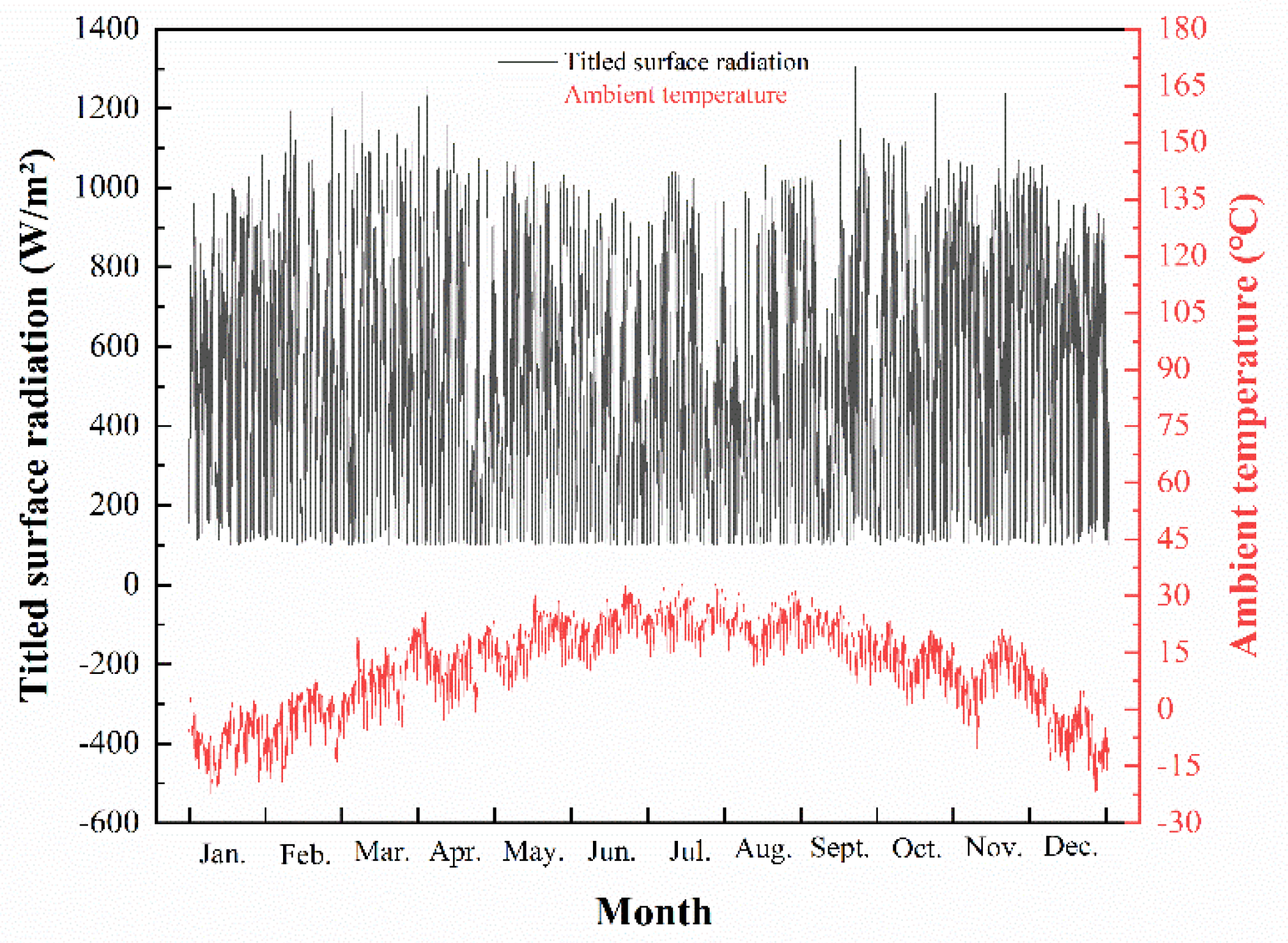
Figure 2.
Annual Proportion of Cumulative Irradiance in Each Irradiance Interval.
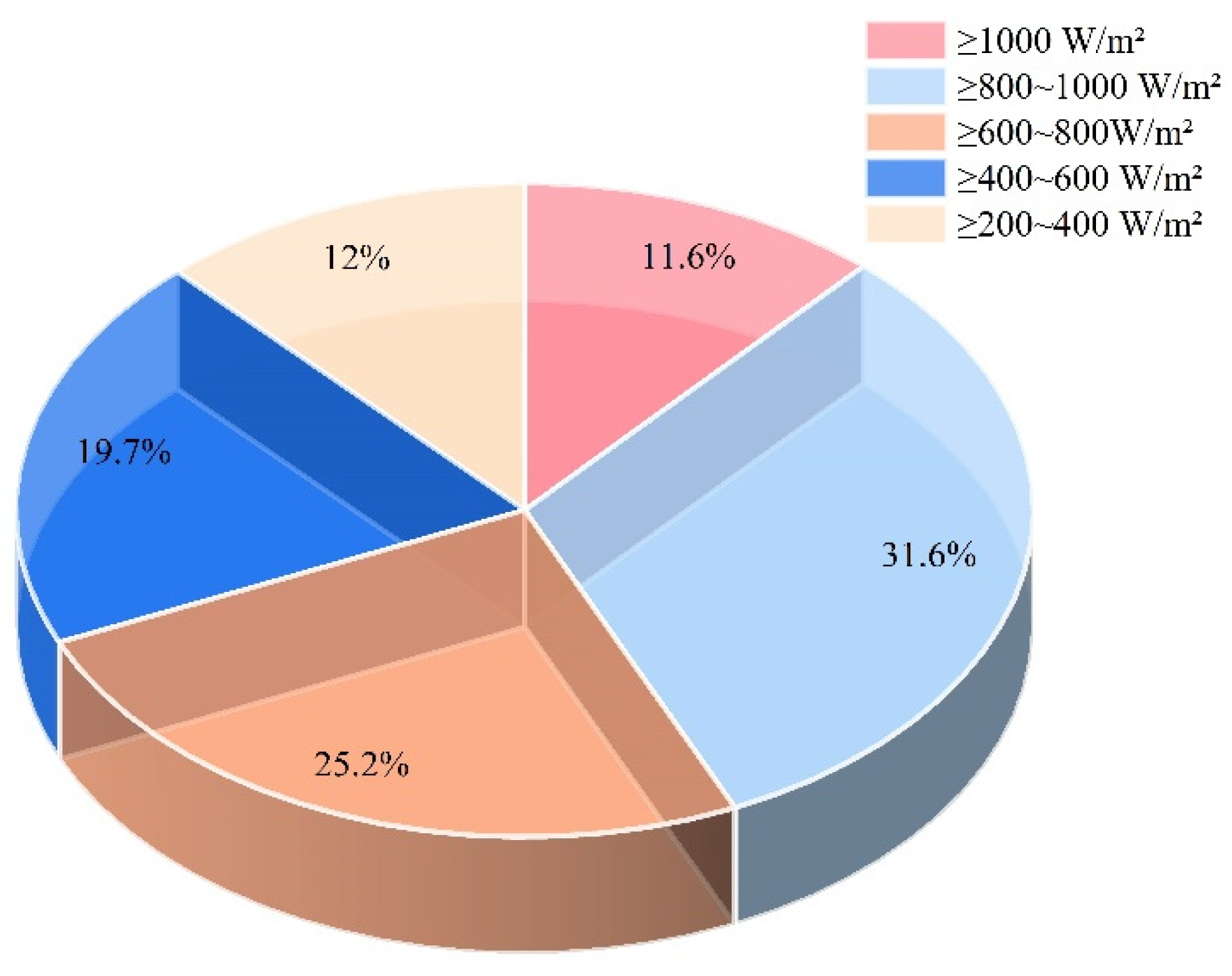
Figure 3.
Annual Average Irradiance and Average Temperature in Each Irradiance Interval.
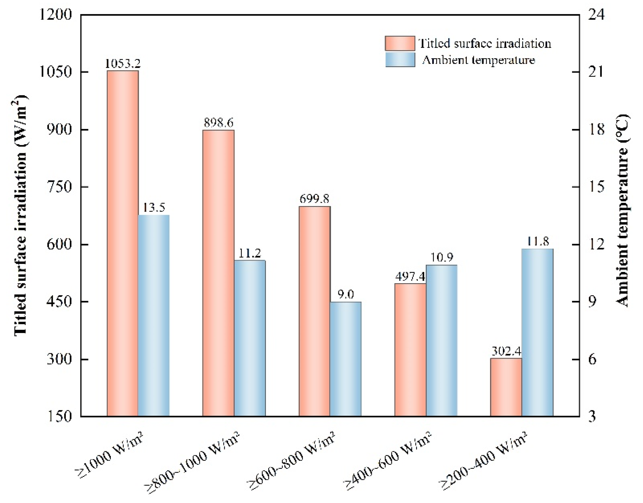
Figure 4.
No-Load Simulink Maximum Power Point Simulation Model.
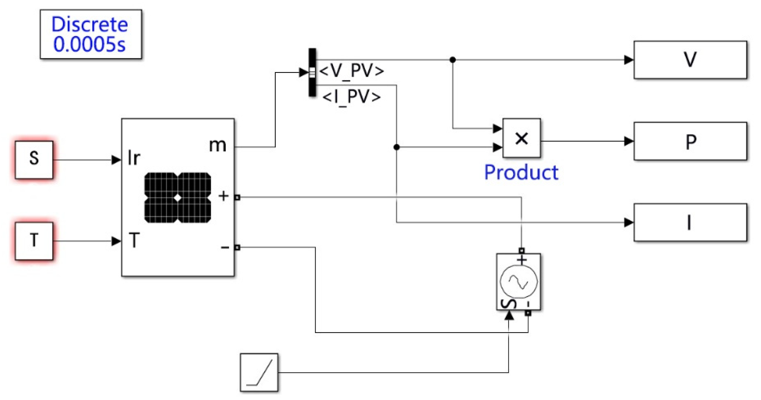
Figure 5.
Maximum Output Power and Internal Resistance at Different Irradiances and Cell Temperatures (No-Load Condition).
Figure 5.
Maximum Output Power and Internal Resistance at Different Irradiances and Cell Temperatures (No-Load Condition).
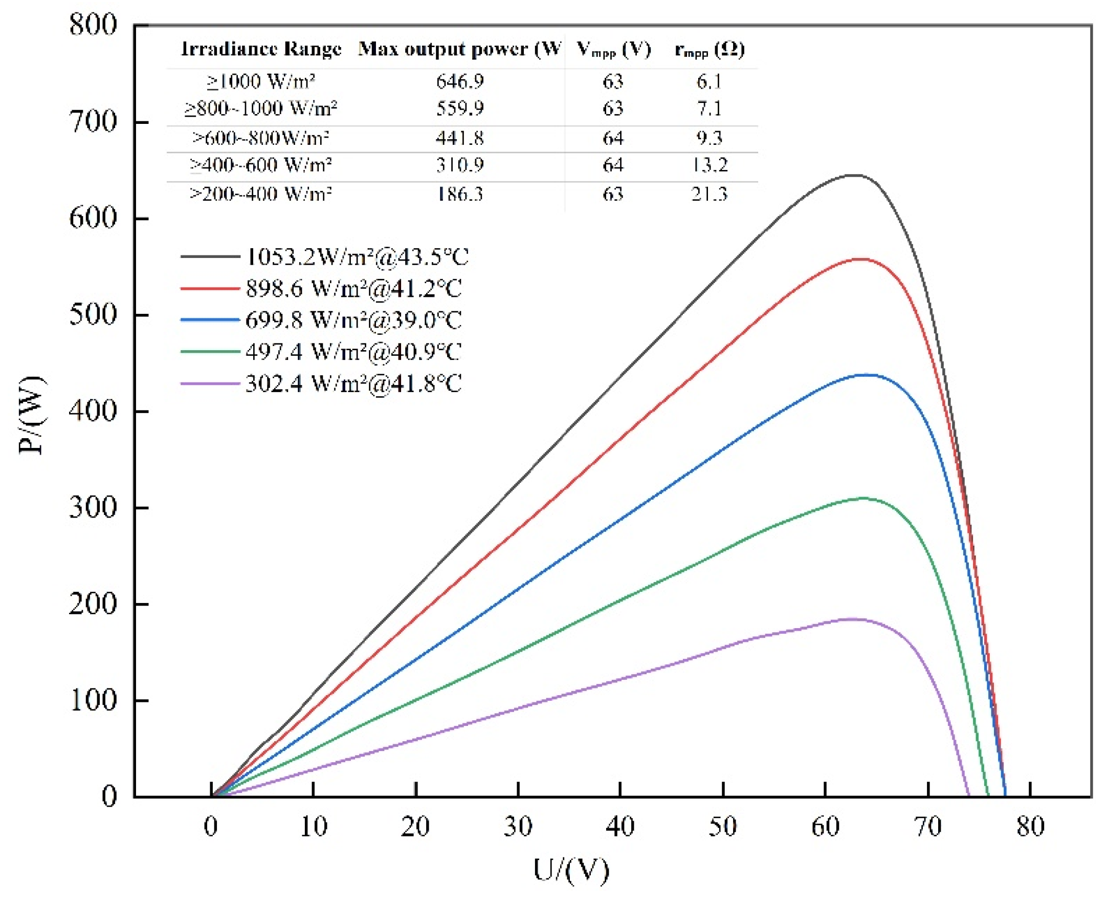
Figure 6.
Loaded Simulink Maximum Power Point Simulation Model.
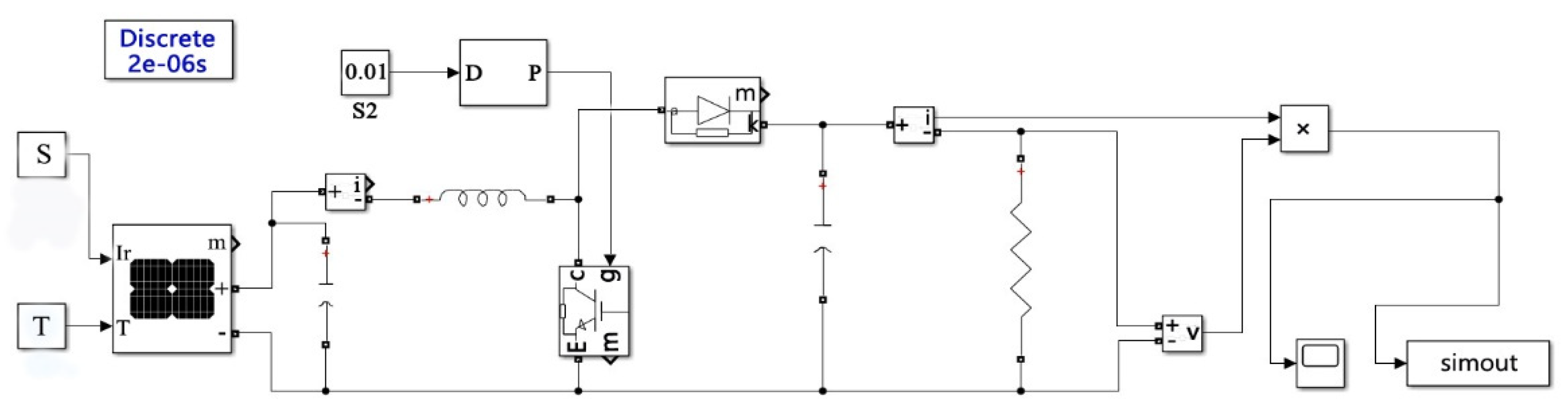
Figure 7.
Maximum Output Power and Internal Resistance at Different Irradiances and Cell Temperatures (Loaded Condition).
Figure 7.
Maximum Output Power and Internal Resistance at Different Irradiances and Cell Temperatures (Loaded Condition).
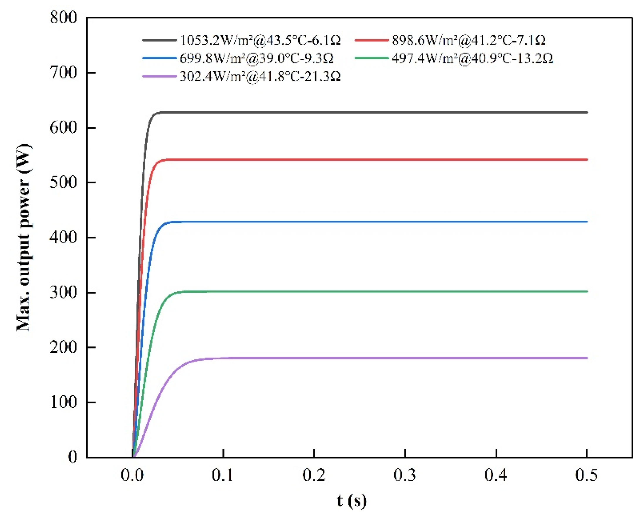
Figure 8.
Comparison of Simulink Maximum Power Output Simulation Models under No-Load and Loaded Conditions.
Figure 8.
Comparison of Simulink Maximum Power Output Simulation Models under No-Load and Loaded Conditions.
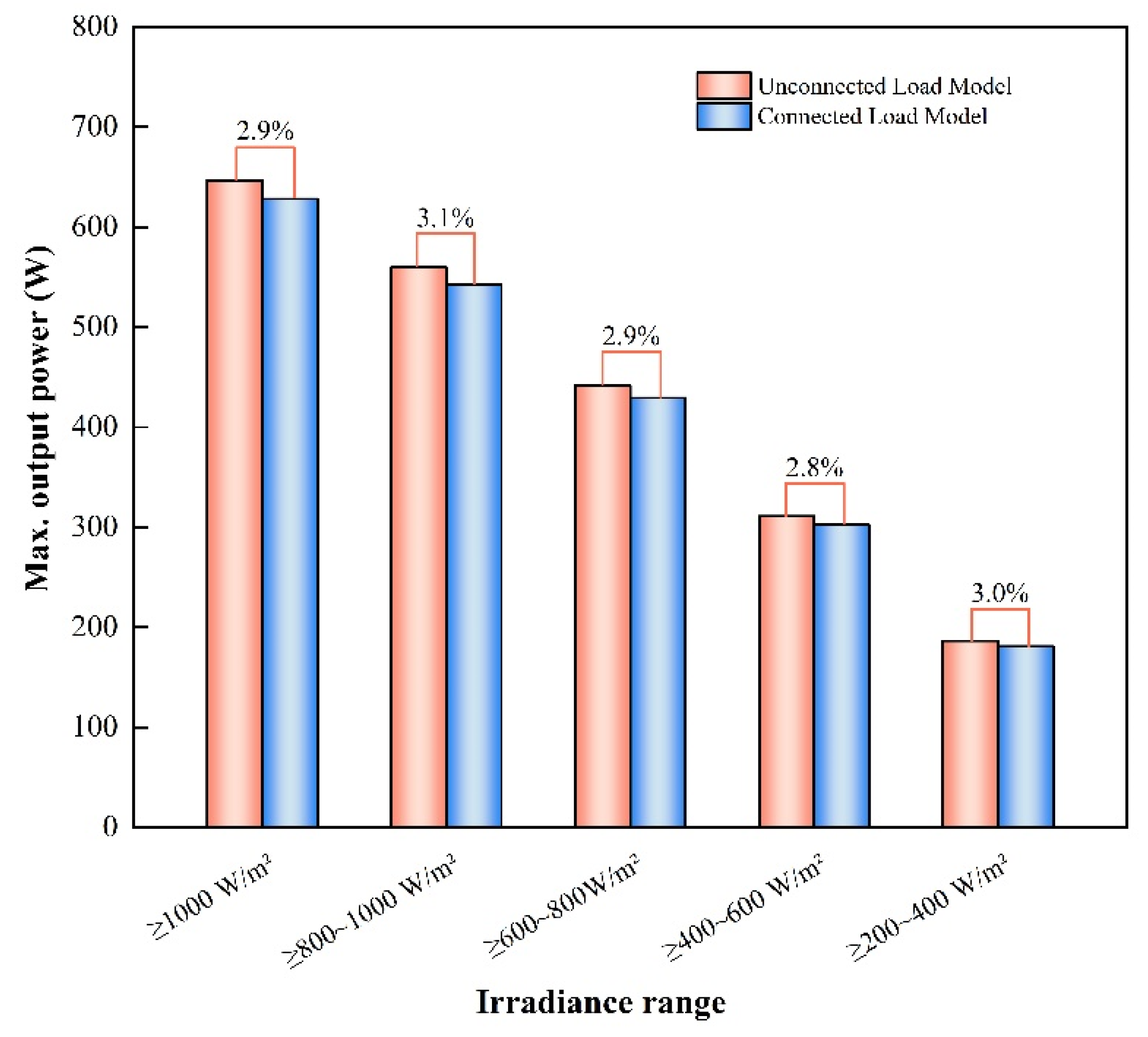
Figure 9.
Artificial Neural Network-Based Maximum Output Power Prediction Model.
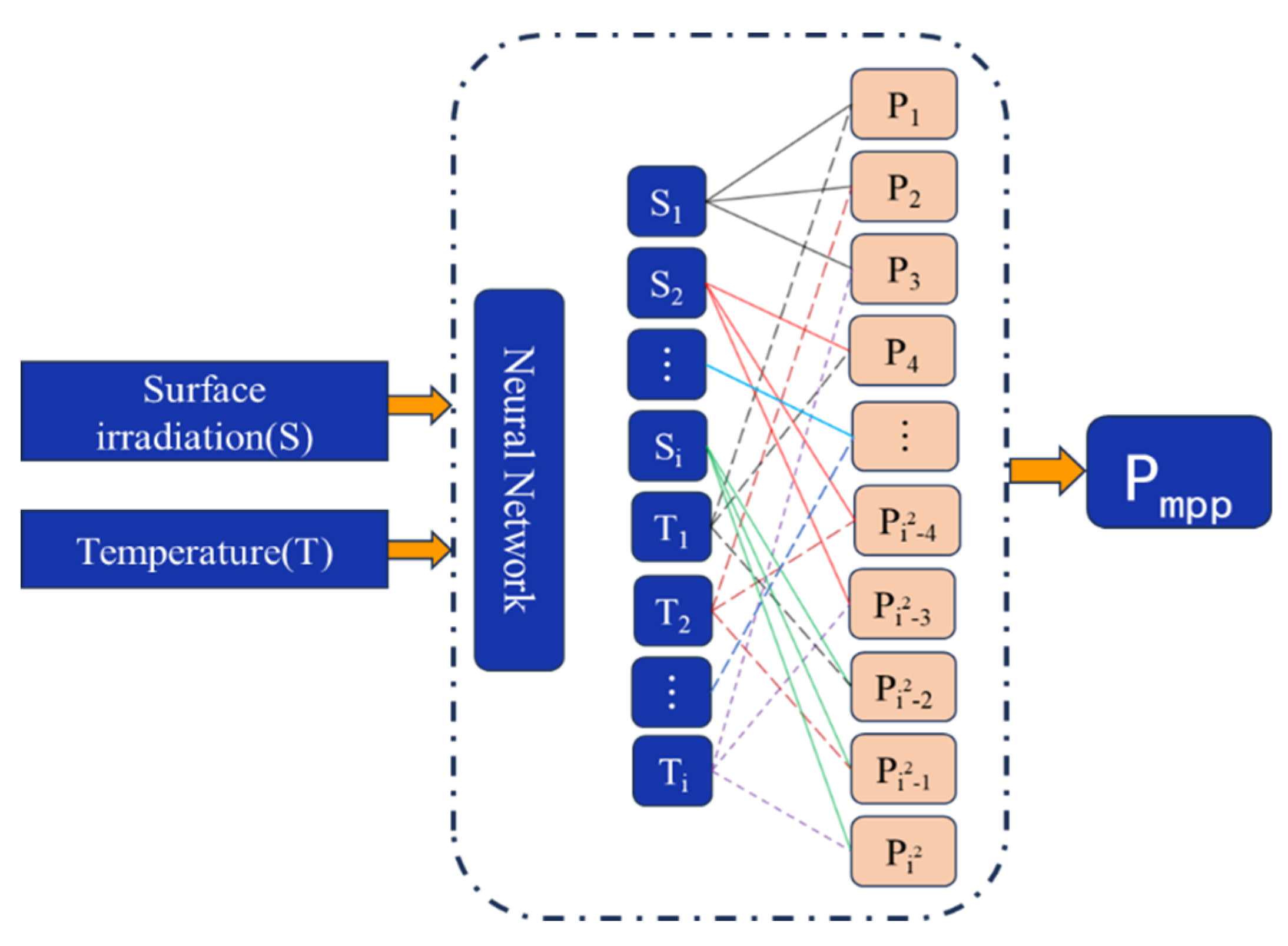
Figure 10.
Maximum Power Point at Irradiance S = 1150 W/m² under Different Temperature Conditions.
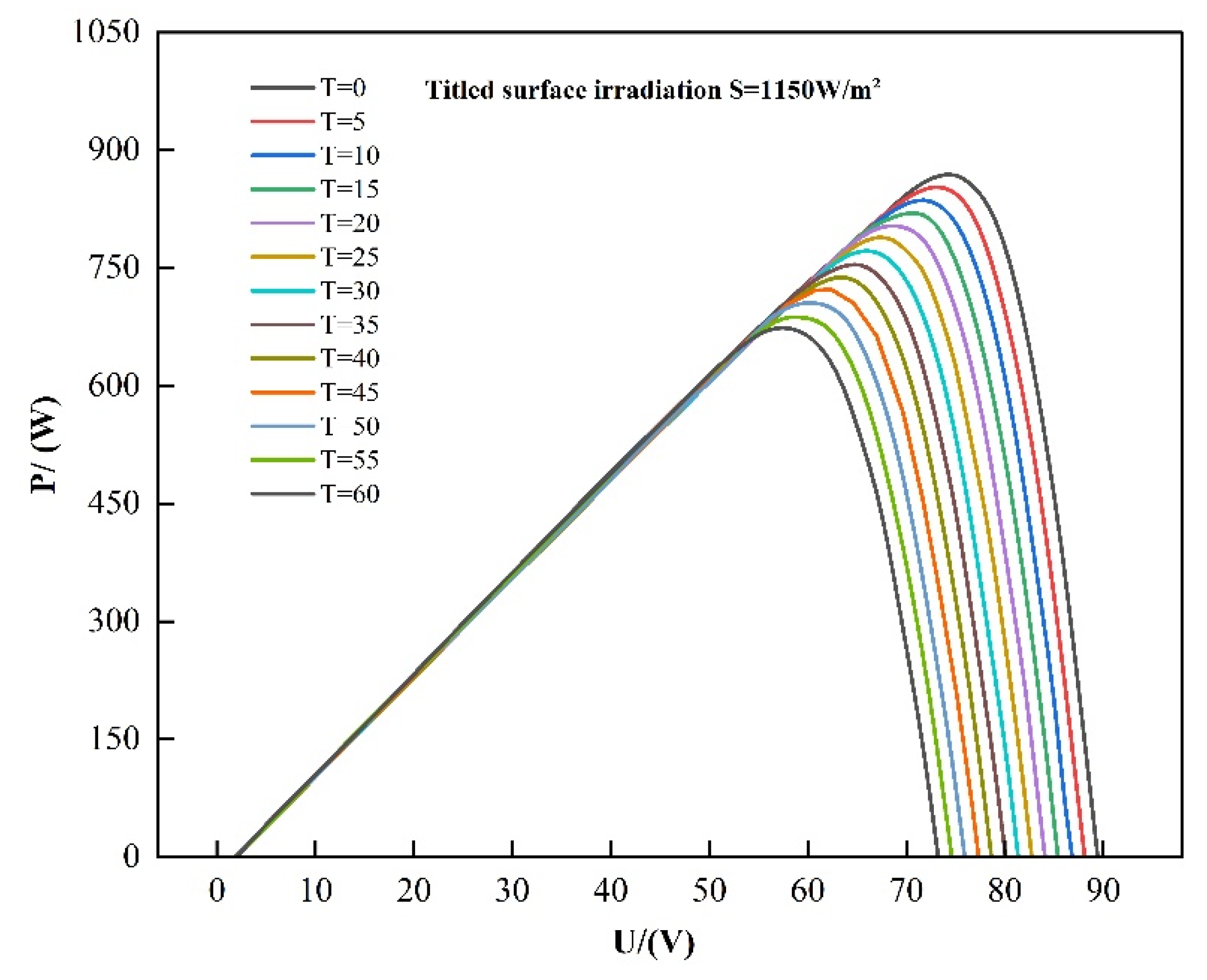
Figure 11.
Traditional Artificial Neural Network Database Dataset.
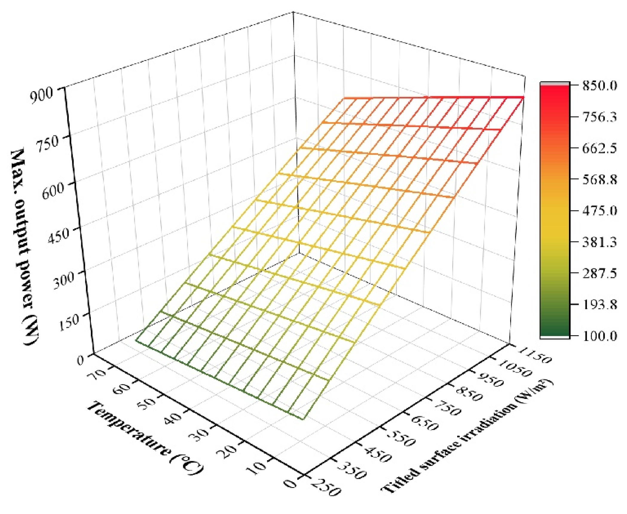
Figure 12.
Operating Principle of the Simplified Control Model for the Adaptive Load Photovoltaic Heating System.
Figure 12.
Operating Principle of the Simplified Control Model for the Adaptive Load Photovoltaic Heating System.
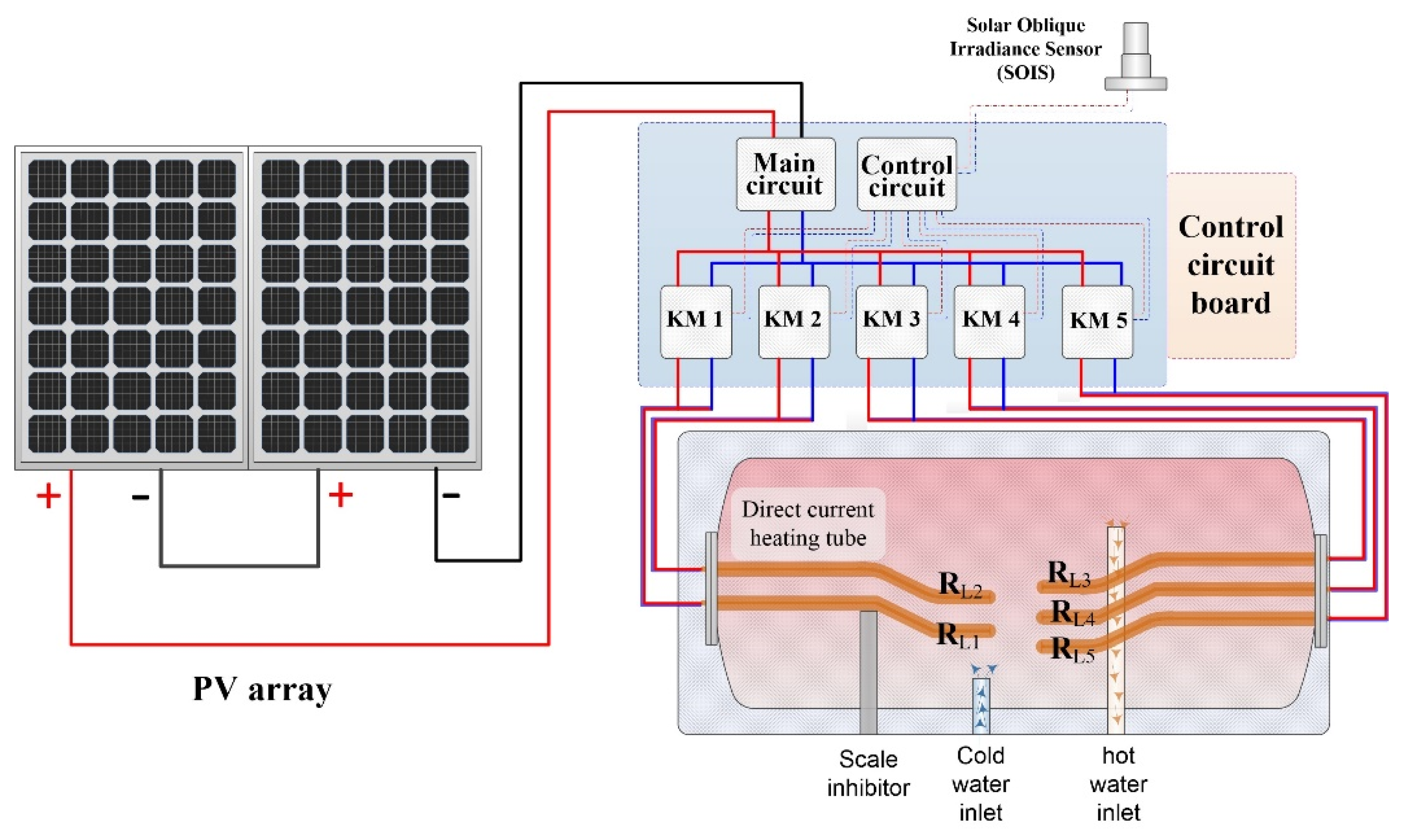
Figure 13.
Annual Cumulative Output Power Comparison between the Conventional and Optimized Artificial Neural Network Prediction Models.
Figure 13.
Annual Cumulative Output Power Comparison between the Conventional and Optimized Artificial Neural Network Prediction Models.
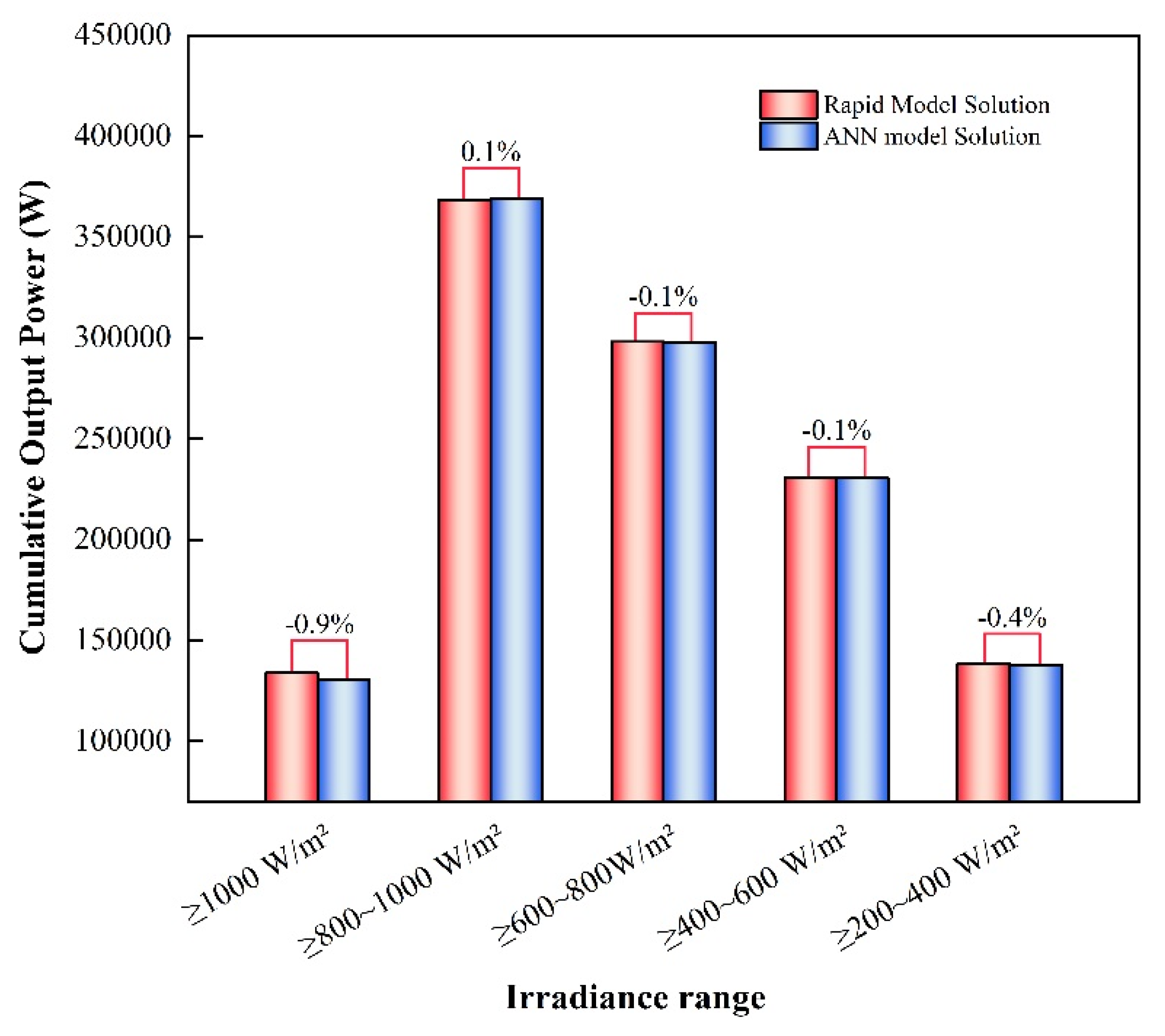
Figure 14.
Optimized Artificial Neural Network Control Model.
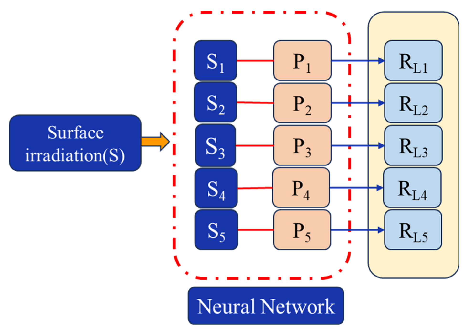
Figure 15.
Traditional Artificial Neural Network Control Model.
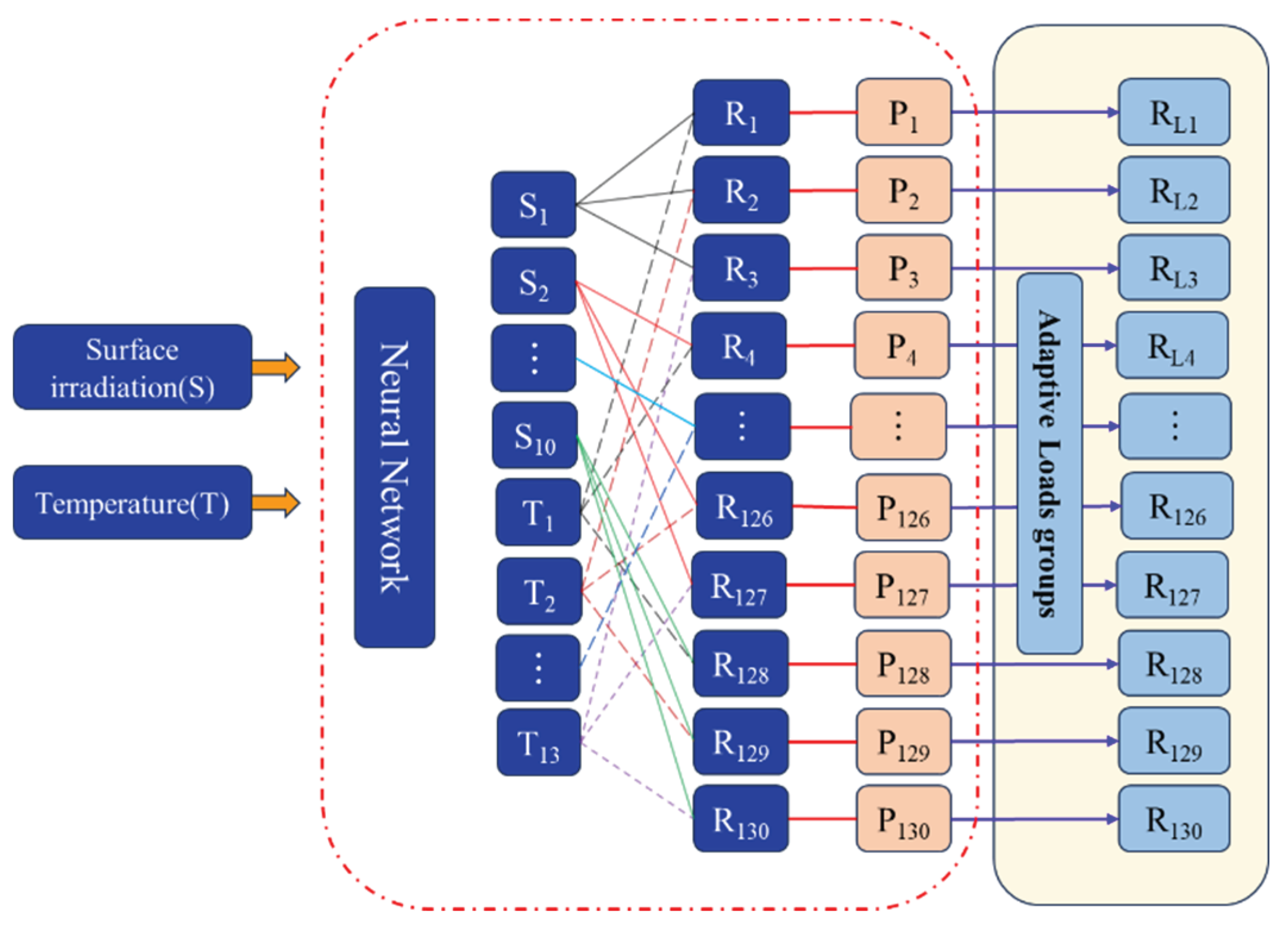

Table 1.
PV array parameters at STC (T=25˚C and S=1000 W/m2).
| Description | Parameter |
| Cells per module (Ncell) | Ncell =60 |
| Maximum power | Pmax = 330 W |
| Voltage at Pmax | Vmpp = 33.5 V |
| Current at Pmax | Impp = 9.85 A |
| Short-circuit current | Isc = 10.26 A |
| Open-circuit voltage | Voc = 41.0 V |
| Temperature coefficient of Voc | -0.330 %/deg.C |
| Temperature coefficient of Isc | +0.049 %/deg.C |
Disclaimer/Publisher’s Note: The statements, opinions and data contained in all publications are solely those of the individual author(s) and contributor(s) and not of MDPI and/or the editor(s). MDPI and/or the editor(s) disclaim responsibility for any injury to people or property resulting from any ideas, methods, instructions or products referred to in the content. |
© 2026 by the authors. Licensee MDPI, Basel, Switzerland. This article is an open access article distributed under the terms and conditions of the Creative Commons Attribution (CC BY) license (http://creativecommons.org/licenses/by/4.0/).
Copyright: This open access article is published under a Creative Commons CC BY 4.0 license, which permit the free download, distribution, and reuse, provided that the author and preprint are cited in any reuse.


