
Submitted:
08 July 2025
Posted:
09 July 2025
You are already at the latest version
Abstract
As global electricity demand increases and concerns over fossil fuel usage intensify, renewable energy sources have gained significant attention. Solar energy stands out due to its low installation costs and suitability for deployment. However, solar power generation remains difficult to predict because of its dependence on weather conditions and decentralized infrastructure. To address this challenge, this study proposes a flexible hybrid ensemble (FHE) framework that dynamically selects the most appropriate base model based on prediction error patterns. Unlike traditional ensemble methods that aggregate all base model outputs, the FHE employs a meta-model to leverage the strengths of individual models while mitigating their weaknesses. FHE is evaluated using data from four solar power plants and is benchmarked against several state-of-the-art models and conventional hybrid ensemble techniques. Experimental results demonstrate that the FHE framework achieves superior predictive performance, improving Mean Absolute Percentage Error by 30% compared to the SVR model. Moreover, the FHE model maintains high accuracy across diverse weather conditions and eliminates the need for preliminary validation of base and ensemble models, streamlining the deployment process. These findings highlight the FHE framework’s potential as a robust and scalable solution for forecasting in small-scale distributed solar power systems.
Keywords:
solar forecasting
; hybrid ensemble
; meta-learning
; meta-modelling
; solar energy systems
; renewable integration
; prediction error analysis
1. Introduction
Despite the continuous rise in global electricity demand, environmental concerns associated with fossil fuel consumption are becoming increasingly critical [1]. This has driven a growing global interest in sustainable energy alternatives, including solar, wind, hydro, and tidal power, collectively termed Renewable Energy Sources (RES) [2,3]. Among these, solar energy stands out due to its widespread availability and suitability for deployment in urban environments [4]. Recent technological advances have significantly improved the conversion efficiency of photovoltaic (PV), positioning solar energy as one of the most rapidly adopted RES options [5,6].
As a result, Solar Power Generation (SPG) has maintained its status as the fastest growing electricity source for the 18th consecutive year, with a 24% increase in capacity compared to 2021—reaching approximately 861 GW globally [7]. However, the inherently variable nature of solar energy presents unique challenges for the integration of the power system [8]. SPG output is highly sensitive to meteorological conditions, leading to significant fluctuations in electricity production. Consequently, accurate solar power forecasting is essential to reduce uncertainty, improve economic viability, and ensure reliable power grid operation through efficient integration of renewable sources [9].
Forecasting in SPG is essential for effective grid integration and is commonly categorized into four primary approaches: physical, statistical, machine learning (ML), and hybrid or ensemble methods [10,11]. In addition to methodological classification, forecasts are also distinguished by their temporal horizon—typically divided into short-term (1 hour to 1 week), medium-term (1 week to 1 month), and long-term (beyond 1 month) predictions [12]. However, it is important to note that these definitions are not universally standardized. For instance, some studies propose a four-tier classification: very short-term (up to 1 day), short-term (up to 2 weeks), medium-term (up to 3 years), and long-term (up to 30 years) [13,14]. This variation highlights the lack of consensus in the literature regarding forecasting horizon definitions.
Physical models rely on mathematical modeling and Numerical Weather Prediction (NWP) systems to simulate the physical processes affecting solar irradiance. These models incorporate variables such as temperature, atmospheric pressure, solar angles and cloud cover [15,16]. They are particularly effective for long-term and large-scale forecasting but require high-resolution environmental data and significant computational resources. Representative examples include radiative transfer models, the P-persistent model, and satellite-based forecasting systems [17,18,19,20]. Despite their accuracy, physical models often face challenges related to calibration, spatial resolution, and model complexity [21].
Statistical approaches use historical data to identify patterns and trends in solar power output [22]. Common techniques include autoregressive (AR), moving average (MA), and their extensions such as ARIMA and SARIMA, which address non-stationarity through differencing [23,24,25,26]. While these models are computationally efficient and relatively easy to implement, they are fundamentally limited by their reliance on linear assumptions and their inability to adapt to rapidly changing environmental conditions.
In the context of SPG, where input variables such as irradiance, temperature, and cloud cover exhibit strong non-linear and non-stationary behavior, statistical models often fail to capture the underlying dynamics accurately [27,28]. Moreover, traditional statistical models are typically static in nature, i.e. they do not incorporate mechanisms for dynamically adjusting to new data patterns or site-specific characteristics. This rigidity makes them unsuitable for distributed solar power systems, where forecast conditions can vary significantly between locations.
Recent advancements in power systems and the exponential growth of data availability have positioned ML and deep learning (DL) as powerful tools for addressing the non-linearity inherent in environmental variables affecting SPG forecasting [29,30]. Regression-based, tree-based, and ensemble models have demonstrated strong performance across various locations and forecasting horizons [31,32,33].
DL models, particularly neural networks such as Recurrent Neural Networks (RNNs) and Convolutional Neural Networks (CNNs), have shown promising results in time series forecasting tasks [34,35]. RNNs are well-suited for sequential data, while CNNs are effective in capturing long-term dependencies [36]. However, the performance of these models is highly dependent on the quality and characteristics of the training data [37]. Variability in forecast accuracy often arises when models are applied across datasets from different PV plants, due to differences in module characteristics, data resolution, and environmental conditions [38].
To overcome the limitations of individual models, hybrid or ensembling approaches that integrate physical, statistical, ML, and DL methods have gained prominence in SPG prediction and forecasting [39,40,41]. These methods often employ ensemble techniques such as boosting [42], bagging [43], and stacked generalization (meta-learning) [44] to combine the strengths of diverse models and reduce prediction uncertainty [45,46]. Boosting and bagging improve performance by reweighting or aggregating predictions from multiple models. Meta-learning, in particular, trains a meta-model on the outputs of several base models, leveraging their complementary strengths while reducing bias and variance [47,48]. Stacking uses cross-validation (CV) to generate meta-features, while blending relies on a hold-out validation set. Though similar in principle, their key distinction lies in how training data is allocated.
Nevertheless, the incorrect model selection can significantly compromise SPG forecast accuracy due to the unique sensitivities of each algorithm, making it crucial to use a model that best fits the given data. Thus, numerous hybrid models have been proposed in this field. For instance, a day-ahead forecasting model combining wavelet transformation, support vector machines (SVM), and particle swarm optimization (PSO) has shown improved accuracy [49]. Other examples include multi-model ensembles that integrate statistical models with artificial neural networks (ANN) using numerical weather data [50], and advanced ML-only hybrids such as ANN-XGBoost-Ridge regression ensembles or the Transformer-LUBE-GRU framework for deterministic day-ahead forecasting [51,52].
Despite their advantages, hybrid models are not without limitations. They may inherit the weaknesses of their constituent models, particularly when less accurate models are included in the ensemble [33]. Moreover, hybrid systems often rely on pre-tested base models, reducing flexibility and adaptability [53]. Even when individual models perform well, their combination does not guarantee improved results, necessitating careful evaluation of the ensemble’s overall performance [54].
These limitations are particularly pronounced in the context of SPG forecasting. One of the key advantages of solar power plants is their geographical flexibility, as they can be deployed in a wide range of environments—including urban, rural, and remote areas—without the spatial and scale constraints typically associated with other energy sources [4]. However, this flexibility introduces significant forecasting challenges due to the resulting heterogeneity in environmental conditions and solar exposure.
Each solar power plant operates under distinct meteorological and operational contexts, which leads to variability in the availability, resolution, and quality of input data. For example, the types and frequency of weather measurements—such as solar irradiance, temperature, humidity, and cloud cover—can differ substantially depending on the location and the instrumentation used [55]. Additionally, the data collection methods and infrastructure (e.g., ground-based sensors vs. satellite data) vary across sites, influencing both the selection and performance of forecasting models.
This distributed and heterogeneous nature of SPG systems demands forecasting models that are both highly adaptable and context-aware. Fixed-output or static models often fail to generalize across different sites, as they are typically optimized for specific data distributions and environmental conditions. As a result, a hybrid ensemble model that performs well for one solar power plant may not achieve the same level of accuracy when applied to another, even if the underlying modeling framework remains unchanged [56]. These challenges underscore the need for flexible ensemble frameworks capable of dynamically adapting to local data characteristics and operational constraints, rather than relying on a one-size-fits-all approach.
An approach that can be tailored to the specific attributes of each site is essential to overcoming the challenge of developing a universally effective forecasting solution. The heterogeneity of environmental conditions, data availability, and system configurations across solar power plants makes it difficult for conventional models to generalize effectively. This underscores the need for a flexible and adaptive forecasting framework capable of dynamically adjusting to site-specific characteristics.
To address these challenges, this study proposes the Flexible Hybrid Ensemble (FHE) Framework, designed to overcome the limitations of traditional hybrid ensemble methods. It reduces reliance on pre-tested model combinations, increases robustness to data variability across different sites, and enables the inclusion of diverse models without compromising overall performance. Furthermore, it adapts dynamically to local environmental and operational conditions, making it particularly well-suited for distributed solar power systems. Key innovations and contributions include:
- 1.
- Selective Model Utilization: The FHE Framework avoids the common pitfall of performance degradation caused by underperforming models by not mandatorily integrating all base models into the final prediction. Instead, it selectively includes only those models that are expected to contribute positively to forecasting accuracy. This eliminates the need for exhaustive pre-testing of individual models and enhances the framework’s adaptability across different sites.
- 2.
- Error-Based Meta-Modeling: A central innovation of the FHE Framework is its use of an error-informed meta-model. Unlike traditional meta-models that rely solely on base model outputs, the FHE meta-model incorporates both historical prediction errors and environmental variables to estimate the expected performance of each base model under specific conditions. This allows the system to dynamically assess and select the most suitable models for each forecasting instance.
- 3.
- Dynamic Base Model Selection: The framework predicts the expected error of each base model for a given input and selects the subset of models most likely to yield accurate predictions. This instance-specific selection enables the ensemble to adapt its configuration in real time, leveraging even models that may perform poorly on average but excel under certain conditions.
The remainder of this paper is organized as follows: Section 2 describes the research design, including the characteristics of the data and the preprocessing steps undertaken. Also, details of the development and implementation of the FHE Framework, with particular emphasis on the methodology through which the meta-model dynamically selects the optimal base models. Section 3 presents the experimental results and performance evaluation. Finally, Section 4 concludes the study and discusses future research directions.
2. Materials and Methods
This section presents the proposed FHE Framework for hourly SPG forecasting. The Framework enhances traditional hybrid ensemble meta-modeling by introducing a dynamic, error-aware model selection strategy. Unlike conventional approaches where the meta-model passively aggregates predictions from all base models, the FHE Framework actively selects the most suitable base models based on forecast-specific meteorological conditions and contextual factors. It comprises several key components: data imputation, preprocessing, feature engineering, and model performance evaluation under different weather conditions.
2.1. Meteorological and Solar Power Data Collection
The meteorological and solar power data used in this study were collected from multiple sources to support the development of a robust forecasting framework. Meteorological observations were obtained1 from the Korea Meteorological Administration (KMA), comprising data from 103 Automated Synoptic Observing System (ASOS) stations and 510 Automatic Weather Station (AWS) stations distributed across South Korea [57]. These datasets include key meteorological variables relevant to solar power forecasting, as listed in Table 1. In parallel, historical SPG data was collected from four distinct PV plants on-site to enable hourly forecasting at each location.
Unlike many previous studies, this work deliberately excludes direct measurements of solar radiation or irradiance from the location site, despite their strong influence on power generation, in order to develop a more universally applicable forecasting model based solely on widely available meteorological data. Specifically, key weather variables were sourced from the ASOS station nearest to each PV plant, with missing values supplemented using data from the more densely distributed AWS network. On average, the distance between each PV plant and its associated ASOS station is approximately 12 kilometers. The geographical locations of the four solar power plants are illustrated in Figure 1. The main characteristics of the four PV plants used in this study are summarized below2:
- Plant 1: Data available from January 2019 to June 2022 at a 1-hour interval. Capacity: 998 kW.
- Plant 2: Data available from January 2019 to June 2022 at a 1-hour interval. Capacity: 369.85 kW.
- Plant 3: Data available from January 2019 to June 2022 at a 1-hour interval. Capacity: 48.3 kW.
- Plant 4: Data available from January 2019 to December 2021 at a 1-hour interval. Capacity: 905 kW.
2.2. Forecasting Hybrid Ensemble: A Modified Framework for Solar Power Prediction
The framework consists of three phases: 1) Data Preparation and Feature Engineering, includes imputation of missing values, feature scaling, and the creation of derived variables such as temporal encodings and astronomical indicators. 2) Base Model Training and Error Profiling, involves training a diverse set of base learners—Random Forest (RF), Support Vector Regression (SVR), LightGBM, XGBoost, Transformer, and Multi-Layer Perceptron (MLP) and profiling their performance using a customized validation strategy. 3) Meta-Model Learning and Inference, a meta-model is trained to predict the expected error of each base model for a given input. During inference, the model(s) with the lowest predicted error are selected to generate the final forecast.
This approach reduces the need for exhaustive pre-selection and allows the inclusion of models that may perform well under specific conditions. A schematic of the FHE workflow is shown in Figure 2.
2.2.1. Data Preparation and Feature Engineering
Prior to model training, the dataset underwent a series of preprocessing steps aimed at improving data quality and enhancing the predictive power of the input features.
Data Scaling
The collected meteorological variables were standardized to ensure consistency across features with varying numerical ranges. This step is essential, as the raw data includes variables that span from small decimal values to large magnitudes, which could otherwise introduce bias during model training. Standardization transforms each feature to have a mean of zero and a standard deviation of one, facilitating more stable and efficient learning, particularly for models sensitive to feature scaling.
Given that the base models employed in this study such as SVR, Multi-Layer Perceptron (MLP), and Transformer are sensitive to the scale of input features, this normalization step is critical. The standardization is expressed in Equation (1).
Where represents the standardized value of the data point, is the original value, is the mean of the training dataset, and is the corresponding standard deviation.
To ensure comparability across solar power plants of varying capacities, the SPG data was normalized by dividing each power output value by the corresponding rated capacity of the plant. This normalization transforms absolute power values into relative performance metrics, enabling unbiased comparisons across heterogeneous plant configurations. The normalized power generation at time step i is defined in Equation (2).
Where represents the normalized power output, is the actual power generated at time i, and denotes the installed capacity of the respective solar power plant. This scaling approach is essential for accurately evaluating operational efficiency and enhancing the robustness of performance forecasting models across diverse system sizes.
Missing Data Imputation
To address missing values in the SPG and meteorological datasets, a hybrid imputation strategy was employed based on the duration of the missing intervals.
-
SPG Data Imputation: For gaps shorter than three consecutive hours, linear interpolation was applied due to its simplicity and effectiveness in short-term continuity. For longer gaps, a historical similarity-based imputation method was used. This approach identifies past time points with similar environmental conditions and substitutes the missing SPG values accordingly. The similarity between the missing time step and a historical candidate is quantified using a weighted distance metric following Equation (3).Where denotes the j-th environmental variable (e.g., solar radiation, sunshine duration, cosine of the hour angle, elevation angle), and is its weight based on correlation with SPG. The historical time point minimizing this distance follows Equation (4)The corresponding SPG value at is then used to impute the missing value. This method leverages domain-specific correlations to enhance imputation accuracy, aligning with practices validated in prior PV forecasting studies [58]
-
Filling Gaps in Meteorological Data: To impute missing values in the ASOS meteorological data associated with each PV plant, the Inverse Distance Weighting (IDW) method was employed. This spatial interpolation technique estimates unknown values based on observations from nearby AWS monitoring stations located within a 10 km radius of each plant. By assigning greater influence to closer stations, IDW ensures that the interpolated values reflect local weather conditions with higher fidelity. Specifically, a missing value at location is estimated as a weighted average of known values from surrounding locations , using Equations (5) and (6).Where is the Euclidean distance between the target location and the known point . The exponent 1.7 was selected to balance the influence of proximity and spatial variability. This method, widely used in geospatial and meteorological applications, effectively captures local variability and has been validated in numerous studies [59].
Both the SPG and meteorological datasets exhibited a low rate of missing values, with less than 0.2% of the data affected. According to prior studies [60,61], missing data rates below 5% are generally considered to have a negligible impact on statistical analyses. Nonetheless, to ensure data continuity and maintain the integrity of subsequent modeling efforts, imputation procedures were applied. Given that the primary objective of this study is not to explore advanced preprocessing techniques, straightforward statistical methods were adopted to address the missing values efficiently and transparently.
Feature Space Expansion via Temporal and Astronomical Transformations
To enhance the predictive accuracy of photovoltaic power generation models, this study expanded the feature space by incorporating both astronomical and temporal transformations. These features were designed to capture the physical dynamics of solar movement and the periodic nature of solar irradiance, complementing the meteorological inputs.
The Skyfield Python library was used to compute solar azimuth and elevation angles for each PV plant location [62]. Additionally, trigonometric transformations of time variables were applied to encode cyclical temporal patterns.
- Azimuth Angle: The azimuth angle, representing the sun’s horizontal position relative to true north, was calculated by mapping the sun’s celestial coordinates to the local horizon of each plant. This computation accounts for the rotation of the Earth and the apparent daily trajectory of the sun. Atmospheric refraction was also considered to improve accuracy [63]. The importance of azimuth angle in PV energy yield has been well established in prior studies, showing its significant influence on annual energy production [64].
- Elevation Angle: The elevation angle, indicating the sun’s vertical position above the horizon, was derived based on the plant’s geographic coordinates and the observation time. Corrections for Earth curvature and atmospheric conditions were included to ensure precision. These angles are critical for modeling solar irradiance on tilted surfaces and are widely used in solar energy modeling [65].
-
Temporal Encoding: To capture the inherent periodicity in solar irradiance, time-related features such as hour of day and month of year were transformed using sine and cosine functions. This approach avoids discontinuities in cyclical variables and enables the model to learn smooth temporal patterns. The transformation is defined in Equations (7) and (8).Where i denotes the time component (e.g., hour, month), and is the total number of units in the cycle (e.g., 24 for hours, 12 for months). This method of encoding cyclical time features has been shown to improve model performance in time-series forecasting tasks.
Incorporating these deterministic features, derived from astronomical and temporal principles, offers a significant advantage over relying solely on meteorological forecasts, which are inherently uncertain [66]. By leveraging physically grounded inputs, the model achieves greater robustness and reliability in forecasting solar power output. A comprehensive list of all features used in this study, including both meteorological and engineered variables, is provided in Table 1.
2.2.2. Base Model Training and Error Profiling
This subsection outlines the training procedure for the base models and the construction of the meta-model within the FHE framework. A customized data splitting strategy is employed to prevent data leakage and to ensure that the meta-model is trained on representative error patterns from the base models.
Data Splitting
The original dataset D is partitioned into two primary subsets:
- (60%): Used exclusively for training the base models.
- (40%): Reserved for error profiling and final evaluation.
Subset is further divided as:
- (70% of ): Used to evaluate the performance of each base model and collect errors for training the meta-model.
- Final Test Set (30% of ): Used for the final assessment of the FHE framework.
This structure (Figure 3) ensures that the meta-model is trained on unseen data relative to the base models, allowing it to learn error patterns without overfitting. The resulting meta-model is then used to select or weight base models dynamically during inference.
Base Model Training
The FHE framework integrates a diverse set of ML and DL models commonly used in renewable energy forecasting, including RF, SVR, LightGBM, XGBoost, Transformer, and MLP [37,67,68,69,70]. All base models are trained using the training subset . The Transformer model is implemented as a regressor using only the encoder architecture. Input features are embedded into a high-dimensional space, and the encoded representation is passed through a fully connected layer to produce the final output. This design is optimized for tabular regression tasks, where sequence generation is not required. Both the Transformer and MLP models are implemented in PyTorch. Details of the model-specific hyperparameters, loss functions, and optimizers are provided in Table 2.
Each base model is trained on the training subset , using input features and corresponding target values . Once trained, the model generates predictions on the validation set . The prediction error for each instance j is then computed as the absolute difference between the predicted and actual values. These individual errors are aggregated to form an error matrix E, which captures the performance of all base models across the validation set following Equations (9) and (10).
Here, K denotes the total number of base models. This matrix serves as the foundation for training the meta-model, which learns to identify the most suitable base models for each input instance based on historical error patterns.
2.2.3. Meta-Model Learning and Forecast Inference
The final stage of the FHE framework involves training a meta-model to predict the expected error of each base model and using these predictions to guide model selection during inference. This process is based on the error matrix generated from the validation subset , along with the corresponding input features.
The meta-model, implemented using the CatBoost regressor, is trained to learn the relationship between input features and the prediction errors of each base model. CatBoost was selected for its ordered boosting mechanism and its ability to handle categorical features effectively through target-based statistics. Hyperparameter optimization was performed using the Optuna library [71]. Once trained, the meta-model is applied to the test set (30% of ) to estimate the expected error for each base model and for each test instance, the two base models with the lowest predicted errors are selected. Their predictions are averaged to produce the final forecast following Equations (11) and (12).
Here, denotes the set of the two base models with the lowest predicted errors for instance j, and is the prediction from base model i. This dynamic selection mechanism allows the FHE framework to adaptively leverage the strengths of different models under varying conditions, improving both accuracy and robustness. The complete algorithmic flow of the FHE framework is summarized in Algorithm 1.
| Algorithm 1 FHE framework: Forecasting with Heterogeneous Ensembles for photovoltaic power prediction. |
|
2.3. Evaluation Metric
To assess the short-term PV forecasting performance, several statistical metrics were employed: Mean Squared Error (MSE), Root Mean Squared Error (RMSE), the coefficient of determination (), Normalized Mean Absolute Percentage Error (NMAPE) and MAE [16,22,36,56]. Additionally, the Normalized MAE (NMAE), as utilized in the Korea Power Exchange (KPX) Renewable generation forecasting system, was included to calculate errors for outputs exceeding 10% of the installed capacity. These metrics are defined in Equations (13)- (18) :
3. Results and Discussion
This section evaluates the performance of the proposed FHE framework across four PV plants, with capacities ranging from 48.3 kW to 998 kW. The results are reported as the average of 10 independent runs (epochs). Performance comparisons are made against standard models and ensemble baselines using multiple error metrics.
3.1. Effect of Feature Engineering on Base Model Accuracy
The impact of engineered features on forecasting accuracy is assessed by comparing four feature scenarios across six base models (RF, SVR, LGBM, XGB, Transformer, and MLP) and four PV plants with varying capacities. The results, averaged over 10 runs, are summarized in Table 3 using the error metrics MSE, NMAE, and . The assessment includes four input configurations, each combining the meteorological data with a different subset of features:
- 1.
- Scenario 1: Meteorological + Radiation + Engineered Features
- 2.
- Scenario 2: Meteorological + Engineered Features (No Irradiance)
- 3.
- Scenario 3: Meteorological (No Irrandiance, No Engineered Features)
- 4.
- Scenario 4: Meteorological + Irradiance (No Engineered Features)
Across all plants and models, the combination of meteorological data, irradiance, and engineered features (Scenario 1) consistently delivers the best performance. This suggests that the inclusion of solar position (azimuth, elevation) and temporal encodings (hour, month) effectively enhances the model’s ability to capture diurnal and seasonal variability. For instance, Random Forest achieves an above 0.86 in all plants, with particularly strong performance in Plants 2 and 4 = 0.897 and 0.898, respectively). Among all models, LGBM slightly outperforms others on average, showing lower MSE and NMAE in most plants.
When direct irradiance measurements are unavailable (Scenario 2), engineered features still contribute significantly to preserving model accuracy. For instance, RF performance only slightly degrades compared to Scenario 1, with dropping by 1–3 percentage points in most plants. This suggests that the engineered features can partially compensate for the absence of irradiance by implicitly capturing solar geometry and temporal dynamics. Interestingly, in Plant 4, MLP outperforms all other models in terms of = 0.860, highlighting its robustness when dealing with incomplete input modalities.
Scenario 3 presents a clear degradation in performance, confirming the critical role of both irradiance and engineered features. All models experience substantial increases in MSE and NMAE, with values dropping dramatically. For example, the for RF in Plant 1 falls from 0.869 (Scenario 1) to 0.255. This trend is consistent across all models and plants, underscoring that meteorological data alone is insufficient for accurate power prediction, especially when solar geometry is not explicitly encoded.
In Scenario 4, the removal of engineered features leads to moderate performance loss compared to Scenario 1, yet models still outperform Scenario 2 in most cases due to the presence of irradiance data. The RF model shows a noticeable drop in in Plant 1 (from 0.869 to 0.833), but maintains reasonable accuracy overall. These results indicate that while irradiance is a strong predictor, engineered features provide additional signal that boosts model generalization, especially in edge cases (e.g., early mornings or cloudy days).
To assess the role of irradiance and engineered features, we compare four feature configurations across all models and plants. Comparing Scenario 1 (all features) to Scenario 2 (engineered features only) reveals only a slight drop in performance, indicating that engineered features can effectively compensate for missing irradiance. For example, the MLP model at Plant 1 maintains nearly identical values (0.853 vs. 0.852), suggesting these features successfully capture relevant solar geometry and temporal patterns. A more dramatic change appears between Scenario 2 and Scenario 3 (neither irradiance nor engineered features), where performance degrades substantially. The RF model at Plant 1, for instance, drops from 0.848 to 0.255, confirming that engineered features are critical when irradiance is unavailable.
Comparing Scenario 3 to Scenario 4 (irradiance only), we find that irradiance improves performance but not as much as engineered features. For instance, SVR at Plant 2 improves from 0.198 to 0.852, yet similar or better performance is often achieved with engineered features alone. The comparison between Scenario 1 and Scenario 4 shows that even when irradiance is available, engineered features still offer additional predictive value. Ensemble models like LGBM and XGB benefit most, with consistent performance gains across plants.
Finally, engineered features are essential for maintaining accuracy in the absence of irradiance and remain beneficial even when irradiance is present, underscoring their value in robust solar energy forecasting.
3.2. Comprehensive Performance Analysis of the FHE Framework
The proposed FHE framework was evaluated using real operational data from PV plants to assess its forecasting accuracy. The analysis focused on the framework’s ability to dynamically select and integrate forecasts from multiple base models based on real-time weather conditions, thereby enhancing prediction reliability. Three baseline settings were considered:
- 1.
- Baseline 1: Each base model was evaluated independently within the FHE framework, providing a reference for standalone performance.
- 2.
- Baseline 2: Conventional hybrid ensemble strategies were applied, including meta-modeling and bagging, which combine forecasts from all base models.
- 3.
- Baseline 3 (FHE): The proposed FHE approach selectively integrates forecasts from the best-performing model for specific conditions, optimizing prediction dynamically.
Figure 4 and Figure 5 further illustrate the FHE framework’s forecasting capability. On clear days (Figure 4), the proposed model not only achieves the highest overall accuracy but also captures peak solar production values with superior precision. Under cloudy conditions (Figure 4), it continues to perform reliably, closely tracking the fluctuations in actual power generation. These findings underscore the FHE framework’s adaptability and robustness across diverse environmental conditions, consistently outperforming individual models and conventional ensembles in both stable and volatile weather scenarios.
Table 4 presents a comprehensive evaluation of the proposed FHE model against individual base models and traditional ensemble approaches (Bagging and Meta-Modeling) across four PV plants with varying capacities and operational contexts.
Across all plants and performance metrics the proposed FHE consistently outperforms all baseline and ensemble methods. Notably, for Plant 1, the FHE achieves the lowest RMSE (65.785 kW), MAE (43.470%), and MAPE (12.923%), while also yielding the highest (0.864), indicating superior fit and error minimization. A similar pattern is observed for Plant 2, where the FHE attains an of 0.906 and a MAPE of just 12.332%, outperforming even the most competitive baselines such as RF and LGBM. Performance gains are especially remarkable in Plant 4, a large-scale system with complex dynamics. The FHE achieves a significant reduction in RMSE (55.568 kW vs. > 59 kW for all others), along with a notably lower MAE (36.535%) and highest (0.902), highlighting its robustness in high-capacity scenarios. In Plant 3, although the magnitude of errors is smaller due to the lower capacity of the plant, the FHE still achieves the best overall scores, indicating its scalability across plant sizes.
Interestingly, while tree-based models such as RF and LGBM perform competitively, especially in Plants 1 and 2, and bagging provides modest gains, neither traditional ensemble approach matches the adaptive advantage of the FHE. Transformer and MLP models generally lag in performance, particularly in overcast or highly variable conditions, as evident from their higher RMSE and MAPE values. These results affirm that the selective and condition-aware nature of the FHE model enables it to leverage the strengths of different base learners under varying conditions, thereby achieving more accurate and reliable short-term solar power forecasts across heterogeneous PV plants.
3.3. Evaluation of the Robustness of the FHE Framework
To rigorously evaluate the robustness and generalizability of the proposed FHE framework, two complementary experiments were designed: (1) variation of test set ratios, and (2) time series CV analysis. Initially, a test set ratio of 12% was adopted to capture sufficient temporal variability while maximizing the training data available for the meta-model. To assess the sensitivity of the FHE’s performance to this choice, additional experiments were conducted with increased test set ratios of 16% and 20%. The results of this analysis are summarized in Table 5.
Across all plants, there was a general trend of increasing error as the test set ratio increases. This is expected, as increasing the size of the test set reduces the amount of data available for training, which can impair model generalization. However, the extent of performance degradation varies by model, suggesting differences in robustness. The proposed FHE framework consistently achieves the lowest MAPE and NMAE scores across all plants and test set configurations, highlighting its superior generalization and robustness. For instance, in Plant 1, MAPE increases only modestly from 12.923% (12%) to 15.079% (20%), which is a smaller increment than observed in other models such as SVR (from 17.328% to 19.786%) or Transformer (from 18.934% to 21.158%).
Individually for each plant, Plant 1 (998 kW) FHE achieves the best MAPE and NMAE scores at all test set sizes, with a strong lead over both individual models and ensemble baselines. Notably, even compared to strong competitors like LGBM and RF, FHE provides a relative error reduction of 12–18% in MAPE. In Plant 2 (369.85 kW), again, FHE outperforms all other models. Interestingly, the gap between FHE and others is slightly larger in this plant, with MAPE improvements of up to 20% compared to SVR or XGB at the 20% test ratio.
In the situation of a low-capacity plant, Plant 3 (48.3 kW), exhibits generally higher errors across all models, likely due to higher variability in small-scale energy production. However, FHE remains the top performer, maintaining MAPE scores 1.5–3 points lower than other models, which is particularly notable given the plant’s challenging characteristics. Finally, in Plant 4 (905 kW), FHE once again dominates in performance. Its MAPE remains under 12.8% even at the highest test ratio, while all other models report MAPE values above 14%, indicating better resilience to reduced training data.
Traditional ensemble methods like Bagging and Meta Ensembles provide improved robustness over single learners (e.g., RF, SVR), but they are consistently outperformed by the FHE framework. This suggests that the design of FHE offers a more flexible and effective mechanism for combining base learners under data variability presumably leveraging adaptive weighting or dynamic ensemble construction. For example, in Plant 4 at 20% test ratio Bagging Ensemble was 14.255% MAPE, Meta Ensemble: 14.978% MAPE and FHE: 12.771% MAPE. This performance gap underlines FHE’s ability to better adapt to structural variations and uncertainties in the input data.
Furthermore, to assess the FHE’s robustness to sequence-dependent biases and its ability to generalize across different temporal segments, a time series split-based CV was performed. Unlike random splits, this approach preserves the temporal order of observations, thereby providing a more realistic simulation of forecasting in unseen future conditions [72]. In this setup, four CV groups were executed, each using a chronologically expanding training window and a test set comprising the most recent 12% of the data. The iterations were defined as follows and the results are presented in Table 6:
- CV 1: Training from 2019-01-01 to 2019-09-13
- CV 2: Training from 2019-01-01 to 2020-05-25
- CV 3: Training from 2019-01-01 to 2021-02-05
- CV 4: Training from 2019-01-01 to 2021-10-18
In CV 1, FHE outperformed all models across all four plants. It achieved the lowest MAPE, NMAE, and the highest scores, with particularly strong results for Plant 4 (MAPE: 16.565%, : 0.869), indicating a highly accurate and robust forecast even with limited training history. Notably, classical machine learning models like LGBM and RF performed competitively, but consistently lagged behind FHE in both magnitude of error and explained variance. As the training set increased in CV 2, all models improved in performance, benefiting from more diverse and comprehensive temporal data. However, the margin by which FHE outperformed others widened. It achieved substantial improvements in accuracy metrics, with Plant 1 showing a remarkable reduction in MAPE to 15.059% and an increase in to 0.874. The Bagging and Meta ensembles provided competitive baselines, demonstrating the effectiveness of aggregation techniques, yet FHE still maintained an edge, particularly in reducing systematic under/over-estimation captured by NMAE.
In CV 3, the gap between models narrowed somewhat, as more historical variation had been captured by the models. Despite this, FHE continued to lead in all metrics across the board. For instance, in Plant 3, FHE obtained the best combination of MAPE: 19.743%, NMAE: 6.044%, and : 0.827, reflecting its resilience in small-capacity scenarios where noise and data imbalance are more pronounced. The Transformer and MLP models showed more volatile performance, suggesting that deep architectures without tailored inductive biases or ensemble mechanisms may overfit or underperform in limited training contexts.
By the final iteration, CV 4, where models had the most extensive training data, performances converged but FHE retained its leadership. For instance, in Plant 4, FHE reported a MAPE of 12.976% and an of 0.919, exceeding even ensemble models. Interestingly, RF and LGBM remained consistently strong contenders across all iterations, especially in early phases, highlighting their robustness and data efficiency. However, their relative gains diminished as the data complexity increased. SVR and MLP consistently underperformed, particularly in larger-capacity plants, likely due to their limited ability to capture nonlinearities or contextual dependencies across temporal segments.
4. Conclusions
This study conducted a comprehensive comparative analysis of the proposed FHE model against a wide range of baseline methods for short-term PV power forecasting. The evaluation spanned four real-world PV plants of varying capacities and employed a robust shuffle-based cross-validation strategy across different temporal windows. The results demonstrate that the FHE model consistently outperforms all baseline models, including traditional regressors (RF, SVR, LightGBM, XGBoost), DL architectures (MLP, Transformer), and ensemble methods (Bagging and Meta-Ensemble), across all evaluation metrics.
Notably, the FHE model exhibited a superior forecasting accuracy, reflected by the lowest MAPE and NMAE values across all plants and cross-validation splits. Also, high explanatory power, achieving the highest scores consistently, indicating a strong ability to capture the underlying data variance. And a robust generalization, with stable performance across different time splits and plant sizes, including challenging cases such as small-scale PV installations with higher noise and variability. While ensemble methods such as Bagging and Meta-Ensemble improved upon individual traditional models, they were still outperformed by FHE, underscoring the effectiveness of its hybrid design. Furthermore, DL models underperformed relative to both ensemble and tree-based methods, suggesting that their complexity may not be fully leveraged in this context, potentially due to data limitations or architecture mismatch.
Another important observation is that forecasting performance tends to degrade for smaller plants, likely due to increased stochasticity in their power generation profiles. Nevertheless, the FHE model maintained its lead even under these more difficult conditions, further reinforcing its versatility and robustness. In conclusion, the FHE model emerges as a reliable, accurate, and scalable solution for PV power forecasting across diverse operating conditions. These promising results suggest its strong potential for deployment in operational settings, where accurate and generalizable energy forecasts are critical for grid stability and energy management.
Author Contributions
Conceptualization, N.S., R.Ch-S., and S.P.; methodology, N.S.; software, N.S.; validation, N.S. and S.P.; formal analysis, N.S. and R.Ch-S.; investigation, N.S.; resources, N.S.; data curation, N.S.; writing—original draft preparation, N.S.; writing—review and editing, N.S., R.Ch-S., K.L., S.P.; visualization, N.S. and R.Ch-S.; supervision, S.P.; project administration, K.L. and S.P.; funding acquisition, S.P. All authors have read and agreed to the published version of the manuscript.
Funding
This work was supported by the National Research Foundation of Korea (NRF) grant funded by the Korea Ministry of Science and ICT (MSIT) (2022R1C1C1013225 and RS-2025-02310080)
Data Availability Statement
The meteorological data used in this study were obtained from the Korea Meteorological Administration (KMA) and are available at: http://www.kma.go.kr/. PV power generation datasets used in the experiments are not publicly available due to commercial restrictions, but may be made available by the authors upon reasonable request.
Acknowledgments
We would like to express our heartfelt gratitude to ourselves for the dedication and perseverance that brought this work to fruition. Our sincere thanks go to our families and friends for their unwavering support and encouragement throughout this journey. We are also deeply grateful to the faculty and staff of the Department of Applied Artificial Intelligence at Seoul National University of Science and Technology for their invaluable guidance and support.
Conflicts of Interest
The authors declare no conflicts of interest.
References
- Tong, D.; Zhang, Q.; Zheng, Y.; Caldeira, K.; Shearer, C.; Hong, C.; Qin, Y.; Davis, S.J. Committed emissions from existing energy infrastructure jeopardize 1.5 C climate target. Nature 2019, 572, 373–377.
- Adaramola, M.S.; Paul, S.S.; Oyewola, O.M. Assessment of decentralized hybrid PV solar-diesel power system for applications in Northern part of Nigeria. Energy for Sustainable Development 2014, 19, 72–82.
- Wu, D.; Zeng, H.; Lu, C.; Boulet, B. Two-stage energy management for office buildings with workplace EV charging and renewable energy. IEEE Transactions on Transportation Electrification 2017, 3, 225–237.
- Lund, P.D.; Mikkola, J.; Ypyä, J. Smart energy system design for large clean power schemes in urban areas. Journal of Cleaner Production 2015, 103, 437–445.
- Victoria, M.; Haegel, N.; Peters, I.M.; Sinton, R.; Jäger-Waldau, A.; del Canizo, C.; Breyer, C.; Stocks, M.; Blakers, A.; Kaizuka, I.; et al. Solar photovoltaics is ready to power a sustainable future. Joule 2021, 5, 1041–1056.
- Lu, H.; Tournet, J.; Dastafkan, K.; Liu, Y.; Ng, Y.H.; Karuturi, S.K.; Zhao, C.; Yin, Z. Noble-metal-free multicomponent nanointegration for sustainable energy conversion. Chemical Reviews 2021, 121, 10271–10366.
- Agency, I.E. World Energy Outlook 2022; International Energy Agency, 2022.
- Kruitwagen, L.; Story, K.; Friedrich, J.; Byers, L.; Skillman, S.; Hepburn, C. A global inventory of photovoltaic solar energy generating units. Nature 2021, 598, 604–610.
- Energy, G.; et al. Western wind and solar integration study. Technical report, Citeseer, 2010.
- Das, U.K.; Tey, K.S.; Seyedmahmoudian, M.; Mekhilef, S.; Idris, M.Y.I.; Van Deventer, W.; Horan, B.; Stojcevski, A. Forecasting of photovoltaic power generation and model optimization: A review. Renewable and Sustainable Energy Reviews 2018, 81, 912–928.
- Wan, C.; Zhao, J.; Song, Y.; Xu, Z.; Lin, J.; Hu, Z. Photovoltaic and solar power forecasting for smart grid energy management. CSEE Journal of power and energy systems 2015, 1, 38–46.
- Ahmed, R.; Sreeram, V.; Mishra, Y.; Arif, M. A review and evaluation of the state-of-the-art in PV solar power forecasting: Techniques and optimization. Renewable and Sustainable Energy Reviews 2020, 124, 109792.
- Hong, T.; Fan, S. Probabilistic electric load forecasting: A tutorial review. International Journal of Forecasting 2016, 32, 914–938.
- Van der Meer, D.W.; Widén, J.; Munkhammar, J. Review on probabilistic forecasting of photovoltaic power production and electricity consumption. Renewable and Sustainable Energy Reviews 2018, 81, 1484–1512.
- Mayer, M.J.; Gróf, G. Extensive comparison of physical models for photovoltaic power forecasting. Applied Energy 2021, 283, 116239.
- Andrade, J.R.; Bessa, R.J. Improving renewable energy forecasting with a grid of numerical weather predictions. IEEE Transactions on Sustainable Energy 2017, 8, 1571–1580.
- Lonij, V.P.; Brooks, A.E.; Cronin, A.D.; Leuthold, M.; Koch, K. Intra-hour forecasts of solar power production using measurements from a network of irradiance sensors. Solar energy 2013, 97, 58–66.
- Zhen, Z.; Pang, S.; Wang, F.; Li, K.; Li, Z.; Ren, H.; Shafie-khah, M.; Catalão, J.P. Pattern classification and PSO optimal weights based sky images cloud motion speed calculation method for solar PV power forecasting. IEEE Transactions on Industry Applications 2019, 55, 3331–3342.
- Janjai, S.; Laksanaboonsong, J.; Nunez, M.; Thongsathitya, A. Development of a method for generating operational solar radiation maps from satellite data for a tropical environment. Solar energy 2005, 78, 739–751.
- Perez, R.; Ineichen, P.; Kmiecik, M.; Moore, K.; Renne, D.; George, R. Producing satellite-derived irradiances in complex arid terrain. Solar Energy 2004, 77, 367–371.
- Aslam, S.; Herodotou, H.; Mohsin, S.M.; Javaid, N.; Ashraf, N.; Aslam, S. A survey on deep learning methods for power load and renewable energy forecasting in smart microgrids. Renewable and Sustainable Energy Reviews 2021, 144, 110992.
- Wang, K.; Qi, X.; Liu, H. Photovoltaic power forecasting based LSTM-Convolutional Network. Energy 2019, 189, 116225.
- Bacher, P.; Madsen, H.; Nielsen, H.A. Online short-term solar power forecasting. Solar energy 2009, 83, 1772–1783.
- Li, Y.; Su, Y.; Shu, L. An ARMAX model for forecasting the power output of a grid connected photovoltaic system. Renewable Energy 2014, 66, 78–89.
- Diagne, M.; David, M.; Lauret, P.; Boland, J.; Schmutz, N. Review of solar irradiance forecasting methods and a proposition for small-scale insular grids. Renewable and Sustainable Energy Reviews 2013, 27, 65–76.
- Vagropoulos, S.I.; Chouliaras, G.; Kardakos, E.G.; Simoglou, C.K.; Bakirtzis, A.G. Comparison of SARIMAX, SARIMA, modified SARIMA and ANN-based models for short-term PV generation forecasting. In Proceedings of the 2016 IEEE international energy conference (ENERGYCON). IEEE, 2016, pp. 1–6.
- Yang, D.; Kleissl, J.; Gueymard, C.A.; Pedro, H.T.; Coimbra, C.F. History and trends in solar irradiance and PV power forecasting: A preliminary assessment and review using text mining. Solar Energy 2018, 168, 60–101.
- Louzazni, M.; Mosalam, H.; Khouya, A.; Amechnoue, K. A non-linear auto-regressive exogenous method to forecast the photovoltaic power output. Sustainable Energy Technologies and Assessments 2020, 38, 100670.
- Wang, K.; Qi, X.; Liu, H. A comparison of day-ahead photovoltaic power forecasting models based on deep learning neural network. Applied Energy 2019, 251, 113315.
- Alcañiz, A.; Grzebyk, D.; Ziar, H.; Isabella, O. Trends and gaps in photovoltaic power forecasting with machine learning. Energy Reports 2023, 9, 447–471.
- David, M.; Ramahatana, F.; Trombe, P.J.; Lauret, P. Probabilistic forecasting of the solar irradiance with recursive ARMA and GARCH models. Solar Energy 2016, 133, 55–72.
- Assouline, D.; Mohajeri, N.; Scartezzini, J.L. Large-scale rooftop solar photovoltaic technical potential estimation using Random Forests. Applied energy 2018, 217, 189–211.
- Khan, W.; Walker, S.; Zeiler, W. Improved solar photovoltaic energy generation forecast using deep learning-based ensemble stacking approach. Energy 2022, 240, 122812.
- Peng, T.; Zhang, C.; Zhou, J.; Nazir, M.S. An integrated framework of Bi-directional long-short term memory (BiLSTM) based on sine cosine algorithm for hourly solar radiation forecasting. Energy 2021, 221, 119887.
- Mellit, A.; Pavan, A.M. Performance prediction of 20 kWp grid-connected photovoltaic plant at Trieste (Italy) using artificial neural network. Energy Conversion and Management 2010, 51, 2431–2441.
- Simeunović, J.; Schubnel, B.; Alet, P.J.; Carrillo, R.E. Spatio-temporal graph neural networks for multi-site PV power forecasting. IEEE Transactions on Sustainable Energy 2021, 13, 1210–1220.
- Gaboitaolelwe, J.; Zungeru, A.M.; Yahya, A.; Lebekwe, C.K.; Vinod, D.N.; Salau, A.O. Machine learning based solar photovoltaic power forecasting: a review and comparison. IEEE Access 2023, 11, 40820–40845.
- Mondal, R.; Roy, S.K.; Giri, C. Solar power forecasting using domain knowledge. Energy 2024, 302, 131709.
- Salman, D.; Direkoglu, C.; Kusaf, M.; Fahrioglu, M. Hybrid deep learning models for time series forecasting of solar power. Neural Computing and Applications 2024, pp. 1–18.
- Duan, M.; Li, K.; Yang, C.; Li, K. A hybrid deep learning CNN–ELM for age and gender classification. Neurocomputing 2018, 275, 448–461.
- Abbes, D.; Martinez, A.; Champenois, G.; Robyns, B. Real time supervision for a hybrid renewable power system emulator. Simulation Modelling Practice and Theory 2014, 42, 53–72. [CrossRef]
- Schapire, R.E. The strength of weak learnability. Machine learning 1990, 5, 197–227.
- Breiman, L. Bagging predictors. Machine learning 1996, 24, 123–140.
- Wolpert, D.H. Stacked generalization. Neural networks 1992, 5, 241–259.
- Antonanzas, J.; Osorio, N.; Escobar, R.; Urraca, R.; Martinez-de Pison, F.J.; Antonanzas-Torres, F. Review of photovoltaic power forecasting. Solar energy 2016, 136, 78–111.
- Shaw, R.; Howley, E.; Barrett, E. An intelligent ensemble learning approach for energy efficient and interference aware dynamic virtual machine consolidation. Simulation Modelling Practice and Theory 2020, 102, 101992. Special Issue on IoT, Cloud, Big Data and AI in Interdisciplinary Domains, . [CrossRef]
- Feng, C.; Cui, M.; Hodge, B.M.; Zhang, J. A data-driven multi-model methodology with deep feature selection for short-term wind forecasting. Applied Energy 2017, 190, 1245–1257.
- Krawczyk, B.; Minku, L.L.; Gama, J.; Stefanowski, J.; Woźniak, M. Ensemble learning for data stream analysis: A survey. Information Fusion 2017, 37, 132–156.
- Eseye, A.T.; Zhang, J.; Zheng, D. Short-term photovoltaic solar power forecasting using a hybrid Wavelet-PSO-SVM model based on SCADA and Meteorological information. Renewable energy 2018, 118, 357–367.
- Ramsami, P.; Oree, V. A hybrid method for forecasting the energy output of photovoltaic systems. Energy Conversion and Management 2015, 95, 406–413.
- Phan, Q.T.; Wu, Y.K.; Phan, Q.D. Enhancing One-Day-Ahead Probabilistic Solar Power Forecast With a Hybrid Transformer-LUBE Model and Missing Data Imputation. IEEE Transactions on Industry Applications 2023.
- Kumari, P.; Toshniwal, D. Extreme gradient boosting and deep neural network based ensemble learning approach to forecast hourly solar irradiance. Journal of Cleaner Production 2021, 279, 123285.
- Emmanuel, T.; Maupong, T.; Mpoeleng, D.; Semong, T.; Mphago, B.; Tabona, O. A survey on missing data in machine learning. Journal of Big data 2021, 8, 1–37.
- Polikar, R. Ensemble based systems in decision making. IEEE Circuits and systems magazine 2006, 6, 21–45.
- Zhang, J.; Zhao, L.; Deng, S.; Xu, W.; Zhang, Y. A critical review of the models used to estimate solar radiation. Renewable and Sustainable Energy Reviews 2017, 70, 314–329.
- Zhang, Y.; Beaudin, M.; Taheri, R.; Zareipour, H.; Wood, D. Day-ahead power output forecasting for small-scale solar photovoltaic electricity generators. IEEE Transactions on Smart Grid 2015, 6, 2253–2262.
- .
- Kim, T.; Ko, W.; Kim, J. Analysis and Impact Evaluation of Missing Data Imputation in Day-ahead PV Generation Forecasting. Applied Sciences 2019, 9. [CrossRef]
- Armanuos, A.M.; Al-Ansari, N.; Yaseen, Z.M. Cross Assessment of Twenty-One Different Methods for Missing Precipitation Data Estimation. Atmosphere 2020, 11. [CrossRef]
- Schafer, J.L. Multiple imputation: a primer. Statistical methods in medical research 1999, 8, 3–15.
- Bennett, D.A. How can I deal with missing data in my study? Australian and New Zealand journal of public health 2001, 25, 464–469.
- Rhodes, B. Skyfield: High precision research-grade positions for planets and Earth satellites generator. Astrophysics Source Code Library 2019, pp. ascl–1907.
- Barnie, T.; Hjörvar, T.; Titos, M.; Sigurðsson, E.M.; Pálsson, S.K.; Bergsson, B.; Ingvarsson, Þ.; Pfeffer, M.A.; Barsotti, S.; Arason, Þ.; et al. Volcanic plume height monitoring using calibrated web cameras at the Icelandic Meteorological Office: system overview and first application during the 2021 Fagradalsfjall eruption. Journal of Applied Volcanology 2023, 12, 4.
- Dhimish, M.; Silvestre, S. Estimating the impact of azimuth-angle variations on photovoltaic annual energy production. Clean Energy 2019, 3, 47–58, [https://academic.oup.com/ce/article-pdf/3/1/47/53678227/zky022.pdf]. [CrossRef]
- Zhang, T.; Stackhouse, P.W.; Macpherson, B.; Mikovitz, J.C. A solar azimuth formula that renders circumstantial treatment unnecessary without compromising mathematical rigor: Mathematical setup, application and extension of a formula based on the subsolar point and atan2 function. Renewable Energy 2021, 172, 1333–1340. [CrossRef]
- Zhao, X.; Liu, J.; Yu, D.; Chang, J. One-day-ahead probabilistic wind speed forecast based on optimized numerical weather prediction data. Energy Conversion and Management 2018, 164, 560–569.
- Prasad, R.; Ali, M.; Kwan, P.; Khan, H. Designing a multi-stage multivariate empirical mode decomposition coupled with ant colony optimization and random forest model to forecast monthly solar radiation. Applied energy 2019, 236, 778–792.
- Yang, H.T.; Huang, C.M.; Huang, Y.C.; Pai, Y.S. A weather-based hybrid method for 1-day ahead hourly forecasting of PV power output. IEEE transactions on sustainable energy 2014, 5, 917–926.
- Li, X.; Ma, L.; Chen, P.; Xu, H.; Xing, Q.; Yan, J.; Lu, S.; Fan, H.; Yang, L.; Cheng, Y. Probabilistic solar irradiance forecasting based on XGBoost. Energy Reports 2022, 8, 1087–1095.
- Yang, J.; He, H.; Zhao, X.; Wang, J.; Yao, T.; Cao, H.; Wan, M. Day-Ahead PV Power Forecasting Model Based on Fine-Grained Temporal Attention and Cloud-Coverage Spatial Attention. IEEE Transactions on Sustainable Energy 2023.
- Akiba, T.; Sano, S.; Yanase, T.; Ohta, T.; Koyama, M. Optuna: A next-generation hyperparameter optimization framework. In Proceedings of the Proceedings of the 25th ACM SIGKDD international conference on knowledge discovery & data mining, 2019, pp. 2623–2631.
- Maldonado, S.; López, J.; Iturriaga, A. Out-of-time cross-validation strategies for classification in the presence of dataset shift. Applied Intelligence 2022, 52, 5770–5783.
| 1 | Data available at: http://www.kma.go.kr/
|
| 2 | The data that support the findings of this study are available from the corresponding author upon reasonable request. |
Figure 1.
Geographical locations of the four photovoltaic (PV) South Korean plants used in the experimental analysis
Figure 1.
Geographical locations of the four photovoltaic (PV) South Korean plants used in the experimental analysis
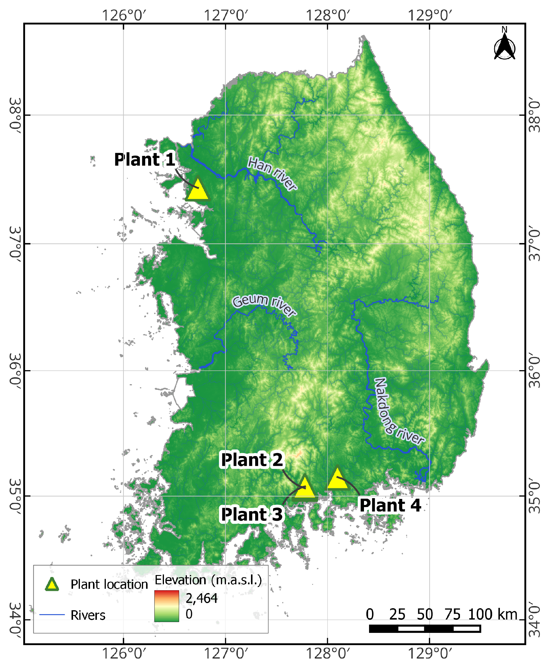
Figure 2.
Architecture of the proposed FHE (Forecasting with Heterogeneous Ensembles) framework.
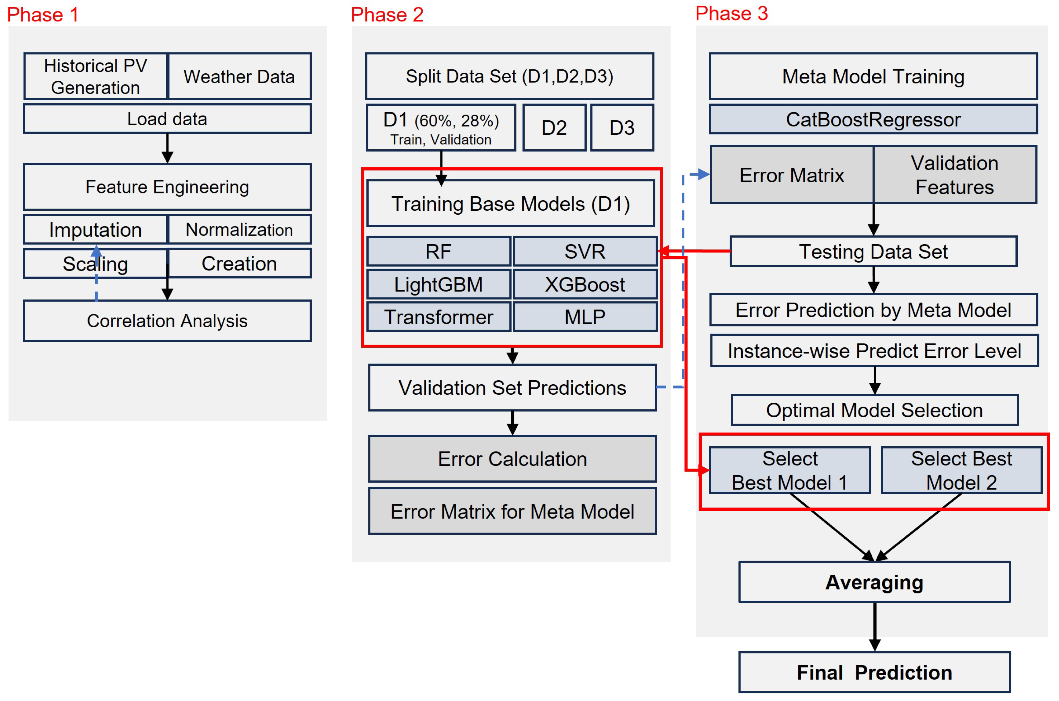
Figure 3.
Data partitioning strategy employed in the FHE framework, illustrating training, validation, and test splits.
Figure 3.
Data partitioning strategy employed in the FHE framework, illustrating training, validation, and test splits.
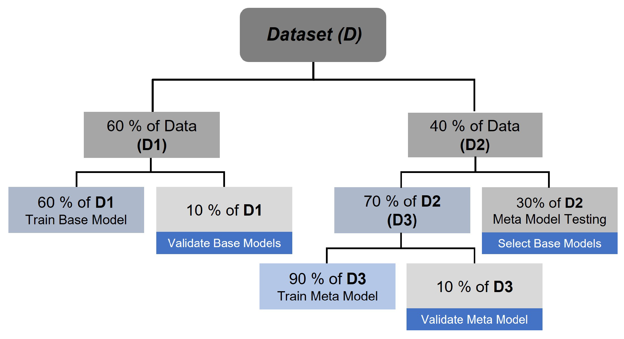
Figure 4.
Forecasting performance of the proposed FHE model on a sunny day at Plant 4. The model accurately captures peak generation periods and overall power output trends.
Figure 4.
Forecasting performance of the proposed FHE model on a sunny day at Plant 4. The model accurately captures peak generation periods and overall power output trends.
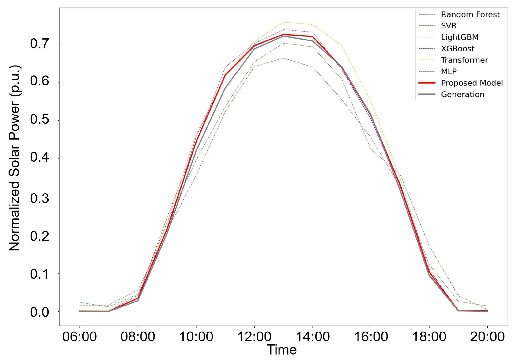
Figure 5.
Forecasting performance of the proposed FHE model on a non-sunny (cloudy or overcast) day at Plant 4. The model effectively tracks power generation variability under less predictable conditions.
Figure 5.
Forecasting performance of the proposed FHE model on a non-sunny (cloudy or overcast) day at Plant 4. The model effectively tracks power generation variability under less predictable conditions.
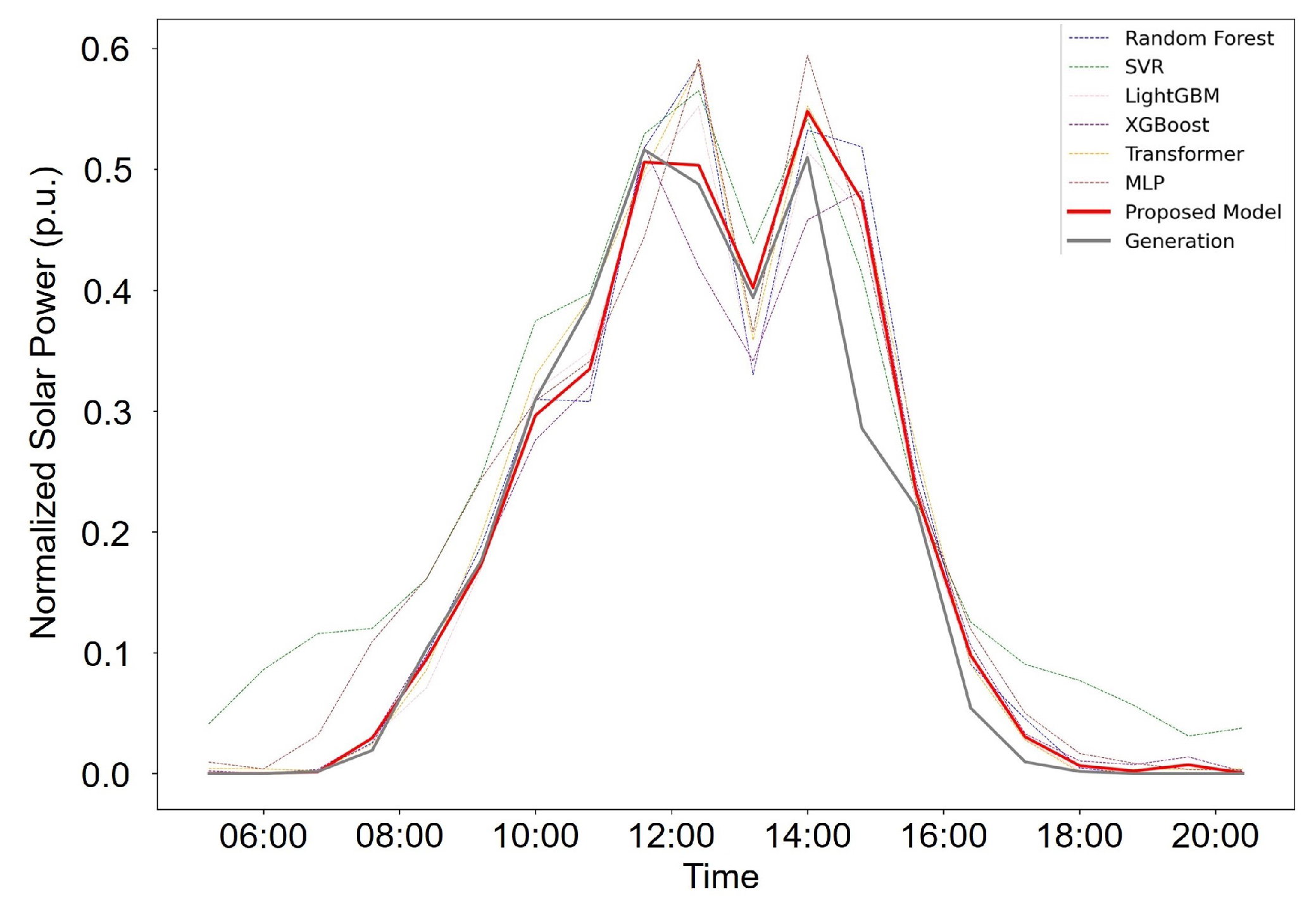

Table 1.
Summary of Input Features Used for Solar Power Generation (SPG) Forecasting, Categorized by Source and Feature Type.
Table 1.
Summary of Input Features Used for Solar Power Generation (SPG) Forecasting, Categorized by Source and Feature Type.
| Engineered | ||||
|---|---|---|---|---|
| Features (Units) | ASOS | AWS | Features | Plant Data |
| Solar Power Generation (kW) | √ | |||
| Temperature (°C) | √ | √ | ||
| Rainfall (mm) | √ | √ | ||
| Wind Speed (m/s) | √ | √ | ||
| Wind Direction (16 cat.) | √ | |||
| Humidity (%) | √ | √ | ||
| Steam Pressure (hPa) | √ | √ | ||
| Site Pressure (hPa) | √ | √ | ||
| Dew Point (°C) | √ | |||
| Sunshine Duration (hr) | √ | |||
| Solar Irradiance (MJ/m²)* | √ | |||
| Visibility (×10 m) | √ | |||
| Azimuth (°) | √ | |||
| Elevation (°) | √ | |||
| Time Sin | √ | |||
| Time Cos | √ |
Table 2.
Hyperparameters and initialization strategies used for each model in the experimental setup.
Table 2.
Hyperparameters and initialization strategies used for each model in the experimental setup.
| Parameter | Value/Method |
|---|---|
| MLP Hidden Layers | 10 |
| Transformer Layers | 3 |
| Transformer Heads | 4 |
| Batch Size | 32 |
| Learning Rate | |
| Loss Function | MAE |
| Optimizer | AdamW |
| Learning Rate Scheduler | ReduceLROnPlateau |
| Initialization Method | He |
| Early Stopping | 10 epochs |
Table 3.
Performance metrics of individual base models across different scenarios and four PV plants.
Table 3.
Performance metrics of individual base models across different scenarios and four PV plants.
| Plant 1 (Capacity: 998 kW) | Plant 2 (Capacity: 369.85 kW) | Plant 3 (Capacity: 48.3 kW) | Plant 4 (Capacity: 905 kW) | ||||||||||||
| Model | MSE (kW, ↓) | NMAE (%, ↓) | (↑) | MSE (kW, ↓) | NMAE (%, ↓) | MSE (kW, ↓) | NMAE (%, ↓) | (↑) | MSE (kW, ↓) | NMAE (%, ↓) | (↑) | ||||
| Scenario 1: Meteorological + Radiation + Engineered Features | |||||||||||||||
| RF | 4.016 | 4.161 | 0.869 | 1.786 | 4.325 | 0.897 | 0.362 | 5.124 | 0.859 | 3.341 | 3.784 | 0.898 | |||
| SVR | 4.364 | 4.690 | 0.858 | 2.006 | 5.413 | 0.885 | 0.364 | 6.004 | 0.858 | 3.930 | 4.888 | 0.880 | |||
| LGBM | 3.998 | 4.198 | 0.870 | 1.788 | 4.493 | 0.897 | 0.365 | 5.305 | 0.857 | 3.427 | 3.790 | 0.896 | |||
| XGB | 4.825 | 4.647 | 0.843 | 1.963 | 4.775 | 0.887 | 0.401 | 5.750 | 0.843 | 3.961 | 4.046 | 0.879 | |||
| Transformer | 6.456 | 5.312 | 0.789 | 2.192 | 4.828 | 0.874 | 0.411 | 5.756 | 0.840 | 3.843 | 4.270 | 0.883 | |||
| MLP | 4.544 | 4.915 | 0.852 | 1.925 | 5.272 | 0.889 | 0.394 | 5.867 | 0.846 | 3.224 | 3.882 | 0.902 | |||
| Scenarios 2: Meteorological + Engineered Features (No Irradiance) | |||||||||||||||
| RF | 4.682 | 4.630 | 0.848 | 2.117 | 4.912 | 0.888 | 0.473 | 7.001 | 0.815 | 4.463 | 4.558 | 0.864 | |||
| SVR | 5.128 | 5.200 | 0.823 | 2.692 | 6.094 | 0.867 | 0.479 | 7.498 | 0.813 | 4.574 | 5.344 | 0.861 | |||
| LGBM | 4.627 | 4.613 | 0.849 | 2.279 | 4.966 | 0.889 | 0.458 | 7.035 | 0.821 | 4.501 | 4.596 | 0.863 | |||
| XGB | 6.114 | 5.308 | 0.800 | 2.472 | 5.265 | 0.877 | 0.460 | 6.988 | 0.820 | 4.881 | 4.950 | 0.851 | |||
| Transformer | 8.001 | 6.087 | 0.739 | 3.196 | 6.000 | 0.828 | 0.619 | 8.434 | 0.758 | 5.076 | 5.138 | 0.845 | |||
| MLP | 4.504 | 4.835 | 0.853 | 2.628 | 6.051 | 0.866 | 0.578 | 8.542 | 0.774 | 4.607 | 5.212 | 0.860 | |||
| Scenarios 3: Meteorological (No Irrandiance, No Engineered Features) | |||||||||||||||
| RF | 22.818 | 12.028 | 0.255 | 11.869 | 14.316 | 0.318 | 2.233 | 17.715 | 0.128 | 19.326 | 11.708 | 0.411 | |||
| SVR | 21.305 | 11.366 | 0.305 | 11.357 | 13.700 | 0.347 | 1.952 | 16.142 | 0.238 | 18.365 | 11.296 | 0.440 | |||
| LGBM | 22.271 | 11.852 | 0.273 | 11.568 | 14.139 | 0.335 | 2.201 | 17.633 | 0.140 | 19.095 | 11.643 | 0.418 | |||
| XGB | 23.544 | 12.379 | 0.232 | 12.043 | 14.292 | 0.308 | 2.348 | 18.139 | 0.083 | 20.727 | 11.986 | 0.368 | |||
| Transformer | 28.878 | 13.332 | 0.057 | 14.643 | 15.379 | 0.158 | 2.574 | 18.873 | 0.056 | 22.502 | 12.303 | 0.314 | |||
| MLP | 23.357 | 12.551 | 0.238 | 11.685 | 14.398 | 0.337 | 2.357 | 18.490 | 0.079 | 20.508 | 12.492 | 0.375 | |||
| Scenario 4: Meteorological + Irradiance (No Engineered Features) | |||||||||||||||
| RF | 5.109 | 5.080 | 0.833 | 1.893 | 5.080 | 0.833 | 0.414 | 5.860 | 0.838 | 4.009 | 4.618 | 0.878 | |||
| SVR | 4.533 | 4.828 | 0.852 | 1.680 | 4.828 | 0.852 | 0.389 | 5.988 | 0.848 | 4.120 | 4.969 | 0.874 | |||
| LGBM | 4.931 | 4.973 | 0.839 | 1.828 | 4.973 | 0.839 | 0.409 | 5.840 | 0.840 | 4.130 | 4.673 | 0.874 | |||
| XGB | 5.883 | 5.527 | 0.808 | 2.180 | 5.527 | 0.808 | 0.437 | 6.033 | 0.829 | 4.856 | 5.076 | 0.852 | |||
| Transformer | 7.699 | 6.466 | 0.749 | 2.853 | 6.466 | 0.749 | 0.435 | 6.097 | 0.830 | 5.068 | 4.999 | 0.46 | |||
| MLP | 4.965 | 4.941 | 0.838 | 1.840 | 4.941 | 0.838 | 0.433 | 6.278 | 0.831 | 4.037 | 4.760 | 0.877 | |||
↑ Greater is better. ↓ Lower is better.
Table 4.
Comparative performance of the proposed FHE model against baseline methods across all PV plants.
Table 4.
Comparative performance of the proposed FHE model against baseline methods across all PV plants.
| Plant 1 (Capacity: 998 kW) | Plant 2 (Capacity: 369.85 kW) | |||||||||
| Model | RMSE (kW, ↓) | MAE (%, ↓) | (↑) | MAPE (%, ↓) | NMAE (%, ↓) | RMSE (kW, ↓) | MAE (%, ↓) | (↑) | MAPE (%, ↓) | NMAE (%, ↓) |
| RF | 68.112 | 46.207 | 0.848 | 14.480 | 4.630 | 26.865 | 18.165 | 0.888 | 13.721 | 4.912 |
| SVR | 71.535 | 51.891 | 0.823 | 17.328 | 5.200 | 29.235 | 22.538 | 0.867 | 16.854 | 6.094 |
| LGBM | 67.957 | 46.036 | 0.849 | 14.773 | 4.613 | 26.698 | 18.367 | 0.889 | 14.284 | 4.966 |
| XGB | 78.115 | 52.975 | 0.800 | 16.417 | 5.308 | 28.141 | 19.473 | 0.877 | 14.668 | 5.265 |
| Transformer | 89.360 | 60.747 | 0.739 | 18.934 | 6.087 | 33.292 | 22.190 | 0.828 | 17.381 | 6.000 |
| MLP | 67.047 | 48.253 | 0.853 | 15.206 | 4.835 | 29.379 | 22.381 | 0.866 | 16.534 | 6.051 |
| Bagging Ensemble | 70.896 | 48.259 | 0.818 | 16.969 | 4.935 | 27.159 | 18.222 | 0.884 | 14.837 | 5.227 |
| Meta Ensemble | 75.387 | 50.242 | 0.814 | 15.213 | 5.034 | 28.541 | 19.993 | 0.873 | 14.731 | 5.406 |
| Proposed FHE | 65.785 | 43.470 | 0.864 | 12.923 | 4.356 | 24.837 | 16.700 | 0.906 | 12.332 | 4.686 |
| Plant 3 (Capacity: 48.3 kW) | Plant 4 (Capacity: 905 kW) | |||||||||
| RF | 4.777 | 3.381 | 0.815 | 18.508 | 7.001 | 63.483 | 41.200 | 0.864 | 14.116 | 4.558 |
| SVR | 4.811 | 3.621 | 0.813 | 19.875 | 7.498 | 64.265 | 48.309 | 0.861 | 17.645 | 5.344 |
| LGBM | 4.702 | 3.398 | 0.821 | 18.751 | 7.035 | 63.754 | 41.549 | 0.863 | 14.447 | 4.596 |
| XGB | 4.714 | 3.375 | 0.820 | 18.677 | 6.988 | 66.391 | 44.745 | 0.851 | 15.346 | 4.950 |
| Transformer | 5.469 | 4.074 | 0.758 | 22.701 | 8.434 | 67.703 | 46.501 | 0.845 | 16.397 | 5.138 |
| MLP | 5.283 | 4.126 | 0.774 | 21.674 | 8.542 | 64.501 | 47.165 | 0.860 | 16.537 | 5.212 |
| Bagging Ensemble | 4.969 | 3.764 | 0.804 | 18.819 | 7.473 | 59.248 | 40.298 | 0.881 | 14.051 | 4.458 |
| Meta Ensemble | 4.642 | 3.370 | 0.826 | 18.509 | 6.978 | 64.441 | 45.384 | 0.860 | 14.809 | 5.015 |
| Proposed FHE | 4.512 | 3.191 | 0.838 | 16.841 | 6.714 | 55.568 | 36.535 | 0.902 | 12.196 | 4.052 |
↑ Greater is better. ↓ Lower is better.
Table 5.
Impact of varying test set ratios on model performance across all forecasting models.
| Plant 1 (Capacity: 998 kW) | Plant 2 (Capacity: 369.85 kW) | |||||||||||
| 12% Testing set | 16% Testing set | 20% Testing set | 12% Testing set | 16% Testing set | 20% Testing set | |||||||
| Model | MAPE (%, ↓) | NMAE (%, ↓) | MAPE (%, ↓) | NMAE (%, ↓) | MAPE (%, ↓) | NMAE (%, ↓) | MAPE (%) | NMAE (%) | MAPE (%) | NMAE (%) | MAPE (%) | NMAE (%) |
| RF | 14.480 | 4.630 | 17.425 | 5.815 | 17.065 | 4.944 | 13.721 | 4.912 | 15.661 | 5.336 | 15.279 | 5.214 |
| SVR | 17.328 | 5.200 | 18.937 | 5.624 | 19.786 | 5.748 | 16.854 | 6.094 | 17.895 | 6.195 | 18.353 | 6.356 |
| LGBM | 14.773 | 4.613 | 16.972 | 4.929 | 17.577 | 5.014 | 14.284 | 4.966 | 14.940 | 5.031 | 15.719 | 5.239 |
| XGB | 16.417 | 5.308 | 18.142 | 5.354 | 18.618 | 5.438 | 14.668 | 5.265 | 15.512 | 5.324 | 16.053 | 5.464 |
| Transformer | 18.934 | 6.087 | 20.326 | 6.196 | 21.158 | 6.339 | 17.381 | 6.000 | 14.144 | 6.159 | 18.849 | 6.345 |
| MLP | 15.206 | 4.835 | 17.564 | 5.276 | 18.206 | 5.386 | 16.534 | 6.051 | 16.326 | 5.641 | 16.855 | 5.805 |
| Bagging Ensemble | 16.969 | 4.935 | 15.955 | 4.705 | 16.667 | 4.829 | 14.837 | 5.227 | 15.128 | 5.226 | 15.269 | 5.170 |
| Meta Ensemble | 15.213 | 5.034 | 16.407 | 4.919 | 17.040 | 5.044 | 14.731 | 5.406 | 15.675 | 5.309 | 16.389 | 5.578 |
| Proposed FHE | 12.923 | 4.356 | 14.600 | 4.459 | 15.079 | 4.585 | 12.332 | 4.686 | 13.486 | 4.843 | 14.079 | 4.968 |
| Plant 3 (Capacity: 48.3 kW) | Plant 4 (Capacity: 905 kW) | |||||||||||
| RF | 18.508 | 7.001 | 19.486 | 7.701 | 19.443 | 7.326 | 14.116 | 4.558 | 14.223 | 4.634 | 14.536 | 4.722 |
| SVR | 19.875 | 7.498 | 20.574 | 7.918 | 20.471 | 7.561 | 17.645 | 5.344 | 17.380 | 5.333 | 17.660 | 5.403 |
| LGBM | 18.751 | 7.035 | 19.585 | 7.694 | 19.199 | 7.247 | 14.447 | 4.596 | 14.371 | 4.638 | 14.499 | 4.670 |
| XGB | 18.677 | 6.988 | 19.861 | 7.705 | 19.954 | 7.426 | 15.346 | 4.950 | 15.248 | 4.986 | 15.370 | 5.002 |
| Transformer | 22.701 | 8.434 | 22.953 | 8.734 | 22.842 | 8.418 | 16.397 | 5.138 | 16.553 | 5.232 | 16.639 | 5.256 |
| MLP | 21.674 | 8.542 | 22.069 | 8.974 | 21.542 | 8.419 | 16.537 | 5.212 | 16.370 | 5.208 | 16.610 | 5.268 |
| Bagging Ensemble | 18.819 | 7.473 | 18.779 | 7.406 | 18.909 | 7.256 | 14.051 | 4.458 | 14.027 | 5.641 | 14.255 | 4.548 |
| Meta Ensemble | 18.509 | 6.978 | 19.679 | 7.768 | 19.672 | 7.375 | 14.809 | 5.015 | 14.686 | 5.055 | 14.978 | 5.038 |
| Proposed FHE | 16.841 | 6.714 | 17.773 | 7.306 | 17.586 | 6.967 | 12.196 | 4.052 | 12.451 | 4.179 | 12.771 | 4.278 |
| ↓ Lower is better. | ||||||||||||
Table 6.
Model performance evaluated using time series cross-validation with shuffled temporal segments.
Table 6.
Model performance evaluated using time series cross-validation with shuffled temporal segments.
| Plant 1 (Capacity: 998 kW) | Plant 2 (Capacity: 369.85 kW) | Plant 3 (Capacity: 48.3 kW) | Plant 4 (Capacity: 905 kW) | ||||||||||||
| Model | MAPE (%, ↓) | NMAE (%, ↓) | (↑) | MAPE (%) | NMAE (%) | MAPE (%) | NMAE (%) | MAPE (%) | NMAE (%) | ||||||
| CV Iteration 1: 2019-01-01 to 2019-09-13 | |||||||||||||||
| RF | 22.522 | 6.070 | 0.762 | 20.442 | 6.107 | 0.802 | 23.768 | 6.910 | 0.735 | 21.449 | 5.796 | 0.815 | |||
| SVR | 28.626 | 7.802 | 0.649 | 31.369 | 8.996 | 0.657 | 36.921 | 10.012 | 0.605 | 27.680 | 7.736 | 0.679 | |||
| LGBM | 21.946 | 5.853 | 0.761 | 22.186 | 6.225 | 0.798 | 26.108 | 7.357 | 0.720 | 17.706 | 5.156 | 0.843 | |||
| XGB | 24.903 | 6.620 | 0.726 | 22.711 | 6.628 | 0.762 | 31.497 | 8.139 | 0.677 | 23.354 | 6.402 | 0.774 | |||
| Transformer | 28.156 | 6.926 | 0.712 | 28.028 | 8.697 | 0.675 | 32.454 | 10.356 | 0.657 | 26.227 | 6.853 | 0.743 | |||
| MLP | 36.166 | 9.225 | 0.532 | 37.291 | 10.371 | 0.539 | 35.113 | 10.525 | 0.610 | 25.843 | 8.007 | 0.651 | |||
| Bagging Ensemble | 21.657 | 5.650 | 0.792 | 22.551 | 6.746 | 0.779 | 23.796 | 6.944 | 0.769 | 19.878 | 5.599 | 0.830 | |||
| Meta Ensemble | 21.418 | 5.978 | 0.760 | 22.455 | 6.472 | 0.779 | 24.547 | 7.277 | 0.734 | 19.704 | 6.250 | 0.761 | |||
| Proposed FHE | 19.138 | 5.236 | 0.816 | 19.968 | 5.801 | 0.816 | 21.911 | 6.425 | 0.779 | 16.565 | 4.795 | 0.869 | |||
| CV Iteration 2: 2019-01-01 to 2020-05-25 | |||||||||||||||
| RF | 17.204 | 5.240 | 0.835 | 18.723 | 6.211 | 0.841 | 18.685 | 6.145 | 0.856 | 15.584 | 4.851 | 0.896 | |||
| SVR | 20.179 | 6.454 | 0.800 | 22.142 | 7.339 | 0.817 | 22.102 | 7.410 | 0.822 | 20.245 | 6.629 | 0.824 | |||
| LGBM | 17.183 | 5.176 | 0.848 | 18.307 | 6.202 | 0.848 | 18.709 | 6.280 | 0.857 | 14.444 | 4.559 | 0.908 | |||
| XGB | 17.917 | 5.478 | 0.827 | 20.053 | 6.593 | 0.829 | 19.968 | 6.586 | 0.848 | 15.659 | 4.878 | 0.889 | |||
| Transformer | 18.611 | 5.516 | 0.805 | 21.171 | 6.785 | 0.816 | 22.384 | 7.497 | 0.789 | 14.735 | 4.830 | 0.880 | |||
| MLP | 20.756 | 6.761 | 0.784 | 20.875 | 7.045 | 0.820 | 21.902 | 7.721 | 0.811 | 19.466 | 6.265 | 0.841 | |||
| Bagging Ensemble | 16.517 | 5.193 | 0.848 | 18.493 | 6.156 | 0.852 | 18.273 | 6.221 | 0.864 | 14.869 | 4.836 | 0.899 | |||
| Meta Ensemble | 16.786 | 5.119 | 0.843 | 18.444 | 6.295 | 0.835 | 19.146 | 6.557 | 0.840 | 14.344 | 4.531 | 0.907 | |||
| Proposed FHE | 15.059 | 4.518 | 0.874 | 16.706 | 5.453 | 0.868 | 16.019 | 5.415 | 0.885 | 13.454 | 4.265 | 0.915 | |||
| CV Iteration 3: 2019-01-01 to 2021-02-05 | |||||||||||||||
| RF | 18.610 | 5.360 | 0.797 | 21.179 | 6.230 | 0.823 | 21.986 | 6.756 | 0.796 | 18.439 | 5.591 | 0.734 | |||
| SVR | 22.465 | 6.250 | 0.766 | 23.864 | 7.387 | 0.780 | 24.043 | 7.135 | 0.783 | 21.889 | 6.504 | 0.787 | |||
| LGBM | 19.515 | 5.491 | 0.796 | 21.841 | 6.437 | 0.814 | 21.865 | 6.789 | 0.792 | 18.879 | 5.732 | 0.772 | |||
| XGB | 20.108 | 5.666 | 0.770 | 22.249 | 6.522 | 0.809 | 22.177 | 6.850 | 0.787 | 20.084 | 6.201 | 0.729 | |||
| Transformer | 22.091 | 6.196 | 0.725 | 23.291 | 6.894 | 0.758 | 24.676 | 8.016 | 0.705 | 21.308 | 6.704 | 0.676 | |||
| MLP | 20.727 | 6.217 | 0.769 | 23.614 | 7.710 | 0.769 | 23.009 | 7.397 | 0.763 | 19.402 | 6.062 | 0.783 | |||
| Bagging Ensemble | 18.320 | 5.275 | 0.810 | 20.601 | 6.241 | 0.825 | 20.856 | 6.592 | 0.802 | 17.944 | 5.570 | 0.797 | |||
| Meta Ensemble | 19.212 | 5.527 | 0.798 | 20.030 | 6.174 | 0.831 | 20.897 | 6.729 | 0.789 | 16.740 | 4.928 | 0.864 | |||
| Proposed FHE | 16.649 | 4.691 | 0.839 | 18.773 | 5.575 | 0.848 | 19.743 | 6.044 | 0.827 | 16.684 | 4.967 | 0.846 | |||
| CV Iteration 4: 2019-01-01 to 2021-10-18 | |||||||||||||||
| RF | 18.964 | 5.200 | 0.783 | 18.798 | 6.126 | 0.828 | 19.630 | 6.899 | 0.776 | 14.920 | 4.657 | 0.874 | |||
| SVR | 21.855 | 6.094 | 0.754 | 21.721 | 7.382 | 0.781 | 21.331 | 7.365 | 0.771 | 17.578 | 5.427 | 0.853 | |||
| LGBM | 19.219 | 5.229 | 0.779 | 18.960 | 6.122 | 0.835 | 20.187 | 7.032 | 0.769 | 14.748 | 4.562 | 0.880 | |||
| XGB | 20.945 | 5.712 | 0.745 | 20.097 | 6.505 | 0.813 | 21.325 | 7.515 | 0.742 | 15.635 | 4.871 | 0.864 | |||
| Transformer | 24.036 | 6.606 | 0.749 | 22.583 | 7.249 | 0.760 | 22.276 | 7.710 | 0.728 | 17.215 | 5.387 | 0.831 | |||
| MLP | 20.208 | 5.570 | 0.763 | 20.738 | 7.097 | 0.801 | 21.668 | 7.976 | 0.738 | 16.484 | 5.505 | 0.847 | |||
| Bagging Ensemble | 19.080 | 5.183 | 0.787 | 18.698 | 6.137 | 0.831 | 19.320 | 6.895 | 0.785 | 14.186 | 4.467 | 0.886 | |||
| Meta Ensemble | 19.376 | 5.550 | 0.776 | 18.806 | 6.054 | 0.837 | 20.0645 | 7.056 | 0.776 | 15.222 | 5.020 | 0.853 | |||
| Proposed FHE | 17.728 | 4.832 | 0.807 | 17.655 | 5.726 | 0.846 | 18.226 | 6.377 | 0.810 | 13.985 | 4.307 | 0.887 | |||
↑ Greater is better. ↓ Lower is better.
Disclaimer/Publisher’s Note: The statements, opinions and data contained in all publications are solely those of the individual author(s) and contributor(s) and not of MDPI and/or the editor(s). MDPI and/or the editor(s) disclaim responsibility for any injury to people or property resulting from any ideas, methods, instructions or products referred to in the content. |
© 2025 by the authors. Licensee MDPI, Basel, Switzerland. This article is an open access article distributed under the terms and conditions of the Creative Commons Attribution (CC BY) license (https://creativecommons.org/licenses/by/4.0/).
Copyright: This open access article is published under a Creative Commons CC BY 4.0 license, which permit the free download, distribution, and reuse, provided that the author and preprint are cited in any reuse.


