
Submitted:
26 January 2026
Posted:
27 January 2026
You are already at the latest version
Abstract
Accurate time series forecasting of sea surface temperature (SST) is essential for understanding the ocean climate system and large-scale ocean circulation, yet it remains challenging due to regime-dependent variability and correlated errors across heterogeneous prediction models.
This study addresses these challenges by formulating SST ensemble time series forecasting aggregation as a stochastic, sample-adaptive weighting problem. We propose a diffusion-conditioned ensemble framework in which heterogeneous base forecasters generate out-of-sample SST predictions that are combined through a noise-conditioned weighting network. The proposed framework produces convex, sample-specific mixture weights without requiring iterative reverse-time sampling. The approach is evaluated on short-horizon global SST forecasting using the Global Ocean Data Assimilation System (GODAS) reanalysis as a representative multivariate dataset. Under a controlled experimental protocol with fixed input windows and one-step-ahead prediction, the proposed method is compared against individual deep learning forecasters and conventional global pooling strategies, including uniform averaging and validation-optimized convex weighting. The results show that adaptive, diffusion-weighted aggregation yields consistent improvements in error metrics over the best single-model baseline and static pooling rules, with more pronounced gains in several mid- to high-latitude regimes. These findings indicate that stochastic, condition-dependent weighting provides an effective and computationally practical framework for enhancing the robustness of multivariate time series forecasting, with direct applicability to global SST prediction from large-scale geophysical reanalysis data.
Keywords:
sea surface temperature (SST) prediction
; GODAS reanalysis data
; multivariate forecasting
; deep learning
; diffusion weighted ensemble
1. Introduction
Sea Surface Temperature (SST) is an important factor to examine in the ocean climate system, as it directly influences air-sea heat exchange, large-scale ocean circulation, and atmosphere-ocean interactions [1]. Fluctuations in SST play a critical role in climate variability, seasonal forecasting, and marine ecosystem dynamics. Consequently, accurate prediction of SST is essential for understanding and monitoring oceanic and climatic processes across multiple temporal scales. Global ocean reanalysis products have been widely used to analyze and model SST variability [2,3]. Among these, the Global Ocean Data Assimilation System(GODAS), developed by the National Oceanic and Atmospheric Administration(NOAA) and the National Centers for Environmental Prediction(NCEP), provides spatially and temporally consistent near-surface ocean temperature fields by assimilating heterogeneous observational data into numerical ocean circulation models. GODAS reanalysis data offer long-term, global-scale SST records and have become a vital data source for ocean climate studies. However, forecasting future SST from global ocean data remains challenging, as SST variability reflects the combined effects of atmospheric forcing, ocean dynamics, and unresolved sub-grid scale processes [4].
Traditional SST prediction approaches have mainly relied on physics-based numerical models or statistical methods. Physics-based models are physically interpretable but computationally expensive and sensitive to uncertainties in initial conditions and parameterization. Statistical approaches are computationally efficient but often assume linearity or stationarity, which limits their ability to represent nonlinear dynamics and long-range temporal dependencies. These limitations have motivated increasing interest in data-driven methods for SST prediction [5]. Recent advances in deep learning (DL) have significantly improved time series forecasting performance. Transformer-based architectures, such as iTransformer, have further improved multivariate relations and time-series dependency modeling through attention mechanisms, while PatchTST enhances long-horizon forecasting by learning informative representations from segmented temporal patches. In contrast, linear decomposition-based models, such as DLinear, provide efficient modeling of trend and seasonal components with low data complexity. Despite these advances, no single model architecture consistently achieves optimal performance across all temporal scales, regions, and forecasting horizons.
SST prediction performance is inherently affected by model uncertainty and data variability. Different models tend to excel under varying temporal regimes, seasonal conditions, and degrees of variability. Relying on a single forecasting model can lead to unstable or suboptimal predictions, particularly under complex oceanic conditions. As a result, ensemble learning has been recognized as an effective strategy to enhance robustness and generalization by integrating the complementary predictive behaviors of multiple models [6,7]. Basic ensemble approaches for SST prediction depend on simple averaging or weighted combinations of deterministic model outputs. While effective to some extent, such approaches do not explicitly model predictive uncertainty or account for the complex, multivariate nature of SST forecasting errors. To address these limitations, probabilistic ensemble frameworks that can represent uncertainty in a principled manner are required [8,9]. Diffusion-weighted generative models provide a robust probabilistic framework for ensemble forecasting by progressively refining noise predictions into coherent predictive distributions, explicitly capturing uncertainty and complex temporal dynamics. Unlike conventional ensemble methods, the diffusion approach can learn the underlying uncertainty structure of model outputs and generate refined forecasts that accurately represent complex temporal variability [10,11,12].
In this study, we propose a diffusion-weighted ensemble framework for SST prediction using GODAS reanalysis data. We first generated base forecasts using heterogeneous DL models, including LSTM, iTransformer, PatchTST, and DLinear, each capturing distinct temporal characteristics of SST variability. The proposed Diffusion-weighted ensemble model integrates these diverse predictions by modeling correlated error patterns and refining them into a unified forecast. This approach allows the ensemble to adaptively exploit the unique strengths of individual models while reducing prediction variance and improving robustness across different forecasting horizons.
- We construct an ensemble composed of diverse model architectures, including LSTM, iTransformer, PatchTST, and DLinear, each capturing complementary temporal characteristics of SST variability, such as long-range dependencies, patchwise temporal patterns, and trend–seasonal components.
- We apply the proposed diffusion-weighted ensemble framework to the multivariate SST GODAS reanalysis data, leveraging consistent global-scale oceanic variables for robust spatiotemporal forecasting.
- We demonstrate that the diffusion-weighted ensemble can effectively refine and combine model predictions by learning their joint uncertainty structure, leading to improved robustness across different forecasting horizons and temporal regimes compared to single models and conventional ensemble approaches.
2. Related Work
2.1. Traditional SST Prediction
Traditional SST prediction has been primarily based on physics-driven numerical ocean models and coupled atmosphere-ocean forecasting systems. Barreto et al. developed and evaluated an operational multigrid ocean forecasting system, demonstrating that physically consistent numerical models can provide reliable SST forecasts over regional domains when properly configured [13]. The main advantage of such systems lies in their physical interpretability and dynamical consistency; however, their performance is sensitive to model resolution and atmospheric forcing errors, leading to persistent regional biases. To mitigate systematic errors in numerical SST forecasts, data-driven bias correction has been explored. Storto et al. proposed a neural network-based surface heat flux correction method embedded in a Nucleus for European Modelling of the Ocean (NEMO) ocean model, showing a significant reduction in SST bias compared to the original configuration [14]. While this hybrid approach improves forecast accuracy without modifying the dynamical core, it remains dependent on the quality and representativeness of the training data and does not explicitly address forecast uncertainty.
In parallel, several studies have concentrated on the refinement and validation of operational forecasting systems. Kong et al. presented validation results for an operational marine forecasting system, highlighting that forecast skill varies substantially across regions and seasons [15]. Although such system-level improvements enhance overall SST performance, the deterministic nature of the forecasts limits their usefulness for probabilistic risk assessment.
The limitations of traditional SST prediction become more evident for extreme events. de Boisséson and Balmaseda investigated the seasonal predictability of marine heatwave occurrence and duration using the European Centre for Medium Range Weather Forecast (ECMWF) seasonal forecast system, showing that while some predictability exists, extreme SST events are often underestimated [16]. Similarly, Koul et al. analyzed the seasonal prediction of marine heatwaves in the Arabian Sea and reported limited reliability for event duration forecasts. These studies indicate that physics-based systems struggle to provide well-calibrated uncertainty information for extremes, motivating the need for probabilistic post-processing frameworks [17].
2.2. DL-Based SST Prediction
DL approaches have been increasingly applied to SST prediction due to their ability to learn nonlinear spatiotemporal dependencies directly from data. Hao et al. investigated ConvLSTM and ST-ConvLSTM models for SST prediction in the South China Sea, systematically analyzing the impact of traditional methods; nevertheless, performance degraded for longer lead times and under dynamically complex conditions [18]. To enhance temporal dependency modeling, Xu et al. proposed a DL framework for short-term global SST prediction using reanalysis data [19]. The study demonstrated that DL models can outperform conventional statistical baselines for global scale forecasting. Nevertheless, the model focused on deterministic point predictions and did not quantify predictive uncertainty, limiting its applicability to risk-aware forecasting.
Attention mechanisms have been introduced to address the limitations of recurrent architectures. Zrira et al. proposed an attention-based BiLSTM model for SST time series forecasting, demonstrating improved long-range temporal feature extraction and higher accuracy than standard LSTM models [20]. Despite these advancements, the method remains primarily time-series-based and does not fully exploit spatial field structures. To enhance spatial modeling, Shi et al. integrated a deformable attention transformer into a ConvLSTM framework, enabling the model to adaptively capture spatial heterogeneity in SST fields [21]. This approach improves prediction accuracy in regions with significant mesoscale variability but introduces increased model complexity and computational cost.
A growing body of work explores multivariate learning approaches. Fu et al. proposed a hybrid model combining LSTM and Transformer architectures, which integrates sequential learning with global attention, demonstrating improved SST prediction across various coastal regions [22]. Yang et al. further indicated that incorporating various physically related variables into a multifactor DL framework enhances robustness under diverse oceanic conditions [23]. However, most multivariate DL studies still emphasize deterministic accuracy metrics and lack probabilistic evaluation.
2.3. Ensemble Techniques for SST Prediction
Ensemble techniques have been widely adopted to enhance SST prediction robustness by integrating the complementary strengths of diverse forecasting models. Dai et al. proposed a stacked generalization ensemble that combines multiple DL predictors through a meta-learning stage, demonstrating that aggregating heterogeneous models can consistently outperform individual predictors in SST forecasting [24]. The key advantage of this approach lies in its ability to exploit complementary error characteristics across models; however, it requires training and maintaining multiple base learners as well as an additional meta-learner, resulting in increased computational and operational complexity. From a modeling perspective, ensemble performance strongly depends on the diversity of base learners. Qian et al. showed that combining predictors that capture different physical and dynamical aspects of the ocean, such as integrating SST with sea surface height anomalies, geostrophic velocities, and wind stress, leads to improved forecast skill in dynamically complex regions [25]. While this multivariate ensemble framework enhances deterministic accuracy, predictive uncertainty is still inferred indirectly from ensemble spread rather than being explicitly modeled.
Ensemble learning has also been applied to SST-related extreme event prediction. Bonino et al. employed machine learning–based ensemble approaches to predict SST variability and marine heatwave occurrence across multiple Mediterranean subregions, highlighting that ensemble aggregation improves robustness under anomalous conditions [26]. Nevertheless, their framework focused on deterministic event prediction, and probabilistic uncertainty was not formally quantified or calibrated. A different ensemble perspective leverages diversity across climate model simulations rather than observational predictors. Boschetti et al.trained ensemble machine learning models exclusively on climate model outputs and demonstrated that machine learning can function as an interpolator among ensemble members, enhancing SST predictability assessment [27]. Although effective in utilizing model diversity, this approach remains dependent on the fidelity of the underlying climate simulations and does not directly address forecast uncertainty calibration.
3. Dataset
In this study, we use ocean temperature and related oceanographic variables obtained from the GODAS. GODAS integrates in situ and satellite observations with a numerical ocean circulation model through data assimilation, providing dynamically consistent estimates of the ocean state [28]. Moreover, NCEP GODAS data are provided by the NOAA Physical Sciences Laboratory (PSL), Boulder, Colorado, USA, on their website at https://psl.noaa.gov. Note that GODAS does not provide a variable explicitly labeled as SST, as shown in Figure 1, which represents the temperature value in GODAS. The dataset includes ocean potential temperature fields at different vertical levels. Hereafter, SST refers to the near-surface potential temperature from GODAS unless otherwise stated; specifically, it denotes the ocean temperature at approximately 5–10 m depth. This near-surface temperature is used as a proxy for SST in reanalysis-based ocean climate and prediction studies and is suitable for analyzing large-scale and seasonal SST variability.
3.1. Data Structure
The GODAS dataset covers the global ocean domain on a regular latitude-longitude grid. Each grid point represents a fixed geographic location for which various oceanographic variables are available as time series. In this study, land grid points where ocean variables are undefined are removed during preprocessing. The data are organized into a spatio-temporal structure in which each sample corresponds to a specific grid point and time index. For each latitude-longitude location, multivariate time series are constructed by stacking the SST and additional oceanographic variables along the temporal dimension. Table 1 summarizes the oceanographic variables provided by the GODAS dataset. Monthly mean data are used throughout the study.
3.2. Data Preprocessing
Several preprocessing steps are applied to the GODAS data prior to model training. Although GODAS provides a wide range of oceanographic variables, not all of them are utilized in this study. Variables are selected to ensure spatial and temporal consistency across the global ocean, which is essential for learning coherent spatio-temporal dependencies in multivariate forecasting models. In particular, variables that exhibit persistent missing values over large contiguous ocean regions or extended temporal intervals are excluded. Such irregular spatial and temporal coverage can introduce structured sparsity, distort local spatio-temporal correlations, and bias the learning of shared representations across grid points and time steps. When incorporated into multivariate time series models, these inconsistencies may lead to unstable training dynamics and degrade generalization by forcing the model to learn from uneven or discontinuous spatio-temporal data. Therefore, we restrict the input set to variables that are spatially continuous and temporally stable over the study period to avoid irregular sampling effects. The final set of input variables used in this study is summarized in Table 2.
To reduce the influence of the mean seasonal cycle and to focus the learning process on interannual and subseasonal variability, anomaly fields are computed for selected variables. For sea surface temperature, surface heat flux, and sea surface height, anomalies are calculated as:
where denotes the raw variable at grid point and time t, and represents the monthly climatological mean for the calendar month m, computed at the same grid point. Other variables, including zonal and meridional ocean currents and upper ocean layer depth variables, are used in their original form.
All input variables are standardized using statistics. Standardization is performed as:
where and denote the mean and standard deviation calculated over the training period. This procedure prevents information leakage from the validation and test periods and improves numerical stability during model training.
For variables that contain missing values, such as ocean mixed layer depth and isothermal layer depth, missing values are retained during preprocessing and set to zero after standardization. Binary masks indicating valid observations are maintained to distinguish missing values during model training.
4. Methodology
This section describes the experimental protocol and the proposed ensemble framework for SST prediction. To ensure a fair and controlled comparison across learning paradigms, we fix the input window and forecasting horizon to and for all models. All approaches share the same preprocessing pipeline and the same train/validation/test split described in Section 3. In addition, all normalization statistics (e.g., mean and standard deviation for z-score standardization) are computed using the training split only and then reused for the validation and test splits to prevent any information leakage.
4.1. Base Forecasting Models
We employ a set of heterogeneous forecasters to capture complementary temporal characteristics of SST variability. Let denote the deep-learning forecasters. To provide additional reference baselines under the short-horizon setting (), we also include two classical machine-learning regressors: Random Forest (RF) and LinearSVR [29,30]. RF is a strong nonlinear tree-ensemble baseline that captures feature interactions with minimal modeling assumptions, while LinearSVR offers scalable learning with a linear kernel on high-dimensional inputs. We define the full set of trained models as . For ensemble construction, however, we restrict candidates to the deep-learning set to focus subset enumeration and adaptive aggregation on models that explicitly learn temporal structure. This restriction ensures that ensemble aggregation operates on forecasts derived from sequence-aware representations rather than flattened lag features. Such sequence-aware models produce forecasts whose errors reflect regime-dependent temporal dynamics, which is essential for learning meaningful, condition-dependent ensemble weights.
4.2. Input Representation for Classical Baselines
Unlike sequence models, classical regressors require fixed-length vectors. For LinearSVR and RF, we convert each sample’s multivariate history into a fixed-dimensional feature vector that matches the temporal context of the deep models. Specifically, the past time steps are concatenated into , where d is the number of input variables. The flattening order across time and variables is kept identical across all experiments to ensure reproducibility. The resulting vectors are standardized using training-set statistics; LinearSVR uses standardized inputs by default, and RF is also trained with the same standardized inputs for consistency.
4.3. Hyperparameter Optimization and Model Selection
For each architecture , we optimize hyperparameters using Optuna [31]. Each Optuna trial is trained on the training split and evaluated on the validation split using a fixed loss metric (e.g., MSE or RMSE). For deep models, we apply early stopping and retain the checkpoint that achieves the lowest validation loss. For LinearSVR and RF, we refit the estimator using the selected hyperparameters on the training split and then obtain validation predictions. After selecting the best configuration for each model, we fix the corresponding forecasters and generate out-of-sample predictions on both the validation and test splits. These predictions are used for (i) single-model comparisons and (ii) deep-learning ensemble construction.
4.4. Validation-Based Ensemble Subset Selection
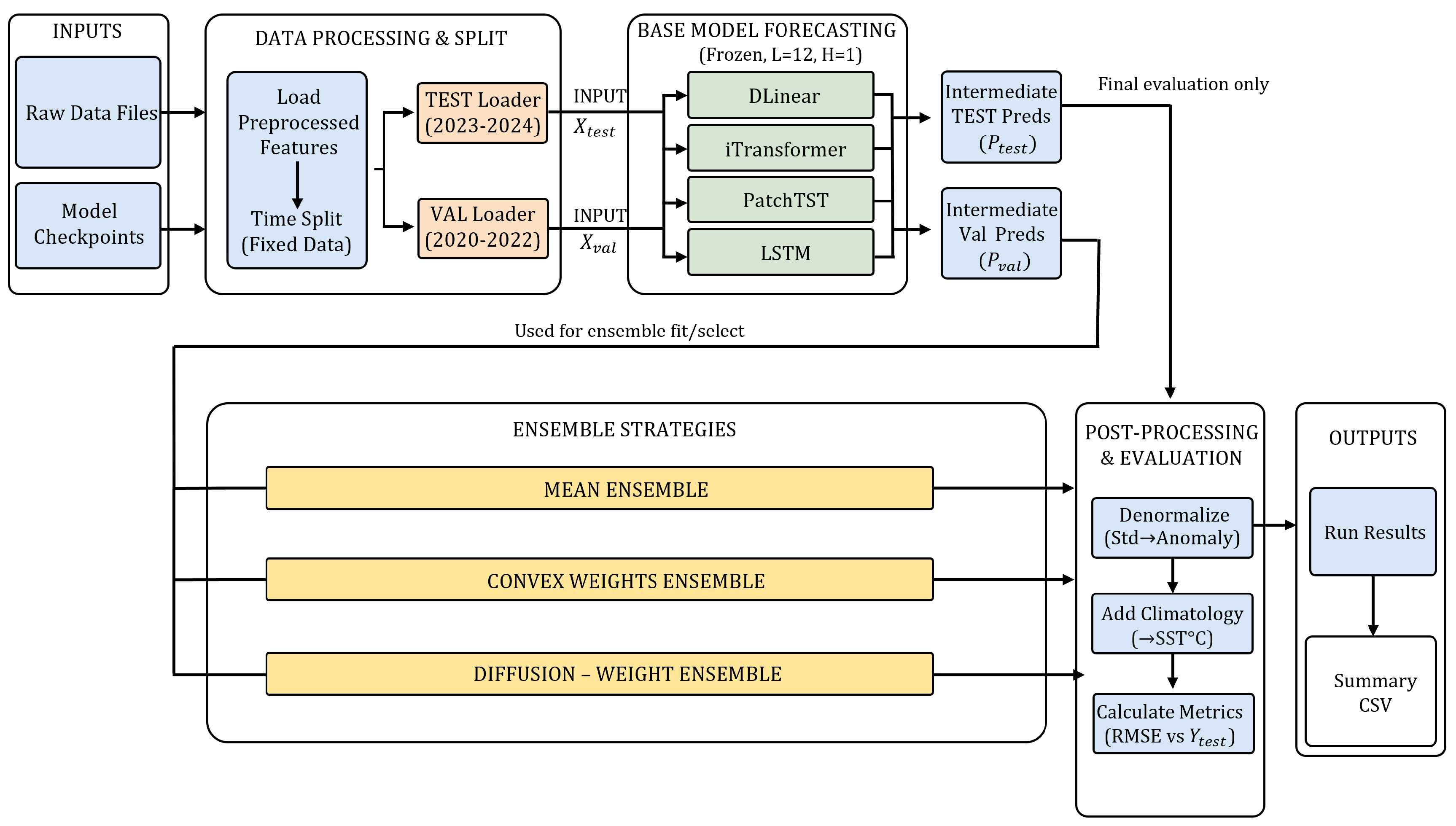
Figure 2 illustrates the overall workflow. Importantly, ensemble fitting and configuration selection are conducted only within the validation split via a meta-train/meta-validation protocol, and the test split is used exactly once for final reporting.
Let denote the collection of out-of-sample base predictions on the validation split. Similarly, let denote the corresponding predictions on the test split. To exploit complementary error patterns among forecasters, we evaluate all non-empty subset ensembles . Let be the number of models in subset S. For each sample, we collect base predictions into a vector
where is the prediction of the i-th base model in S and y is the ground-truth target. When , the ensemble reduces to the corresponding single model. When , we compare multiple aggregation rules, including uniform averaging, validation-optimized convex weighting, and the proposed Diffusion-weighted ensemble. To reduce overfitting during ensemble selection and to avoid any leakage from the test split, we adopt a two-stage protocol on the validation split. Concretely, we first fit any ensemble parameters on a meta-train subset, then select the best subset and aggregation rule using a disjoint meta-validation subset. The selected configuration is subsequently refit using the full validation split, and the test split is used exactly once for final reporting. We denote these two disjoint subsets as and (both drawn from the validation split), where ensemble parameters are fitted on and configurations are selected based on performance on .
Figure 2.
Overview of the deep-learning ensemble pipeline. Base forecasters (DLinear, iTransformer, PatchTST, LSTM) generate out-of-sample predictions on the validation split (). Ensemble parameters and the best subset/aggregation rule are selected using a meta-train/meta-validation protocol within validation only, and the selected ensemble is then applied once to the test predictions () for final evaluation.
4.5. Aggregation Rules for Sample-Adaptive Ensemble Forecasting
Ensemble performance depends not only on which base forecasters are included but also on how their outputs are combined. Because different forecasters can exhibit correlated errors and regime-dependent strengths (e.g., seasonal vs. interannual variability), there is no single universally optimal pooling strategy. Therefore, we compare three aggregation rules with increasing modeling capacity and adaptivity to (i) establish a transparent baseline, (ii) test whether a global, validation-fitted combination improves over naive averaging, and (iii) evaluate whether sample-adaptive weighting yields additional gains. Concretely, we consider: (1) a uniform mean as a strong, assumption-light reference; (2) validation-optimized convex weights (linear pool) as a classical forecast-combination method that learns a global mixture while mitigating overfitting via nonnegativity and sum-to-one constraints; and (3) the proposed diffusion-weighted rule as a sample-adaptive mechanism that can vary mixture weights across different oceanic conditions. This controlled comparison allows us to attribute improvements to the aggregation strategy itself rather than to changes in base models, and it clarifies the value of sample-adaptive weighting beyond conventional global pooling.
Given a subset S of K base forecasters and the corresponding prediction vector , the uniform mean ensemble is defined as
As a stronger global pooling baseline, we also learn nonnegative convex weights on the meta-train split:
and predict by . Here, for each sample n, denotes the stacked base predictions and denotes the corresponding ground-truth target (each sample can be interpreted as a specific spatiotemporal point, e.g., a grid cell at a given time). While convex weighting provides a simple yet competitive global combination rule, it cannot adapt to sample-specific conditions. To obtain sample-adaptive mixture weights, we propose a diffusion-weighted ensemble inspired by diffusion probabilistic models [32]. Specifically, we perturb the base prediction vector via a forward noising process:
where , T is the number of diffusion steps, is a predefined noise schedule, , and for we define (with by convention). Given the noised input , we learn a noise-conditioned weighting network that takes the concatenated input and outputs K logits, which are converted into mixture weights via
where denotes a sinusoidal embedding of the diffusion step t. The final forecast is computed as a convex combination of the clean base predictions:
Figure 3.
Architecture of the proposed diffusion-weighted ensemble. Given the clean base prediction vector , we apply forward noising to obtain and use a noise-conditioned weighting network to produce convex weights via softmax. At inference, Monte-Carlo averaging over multiple draws yields the final weights , which are applied to to compute the final forecast .
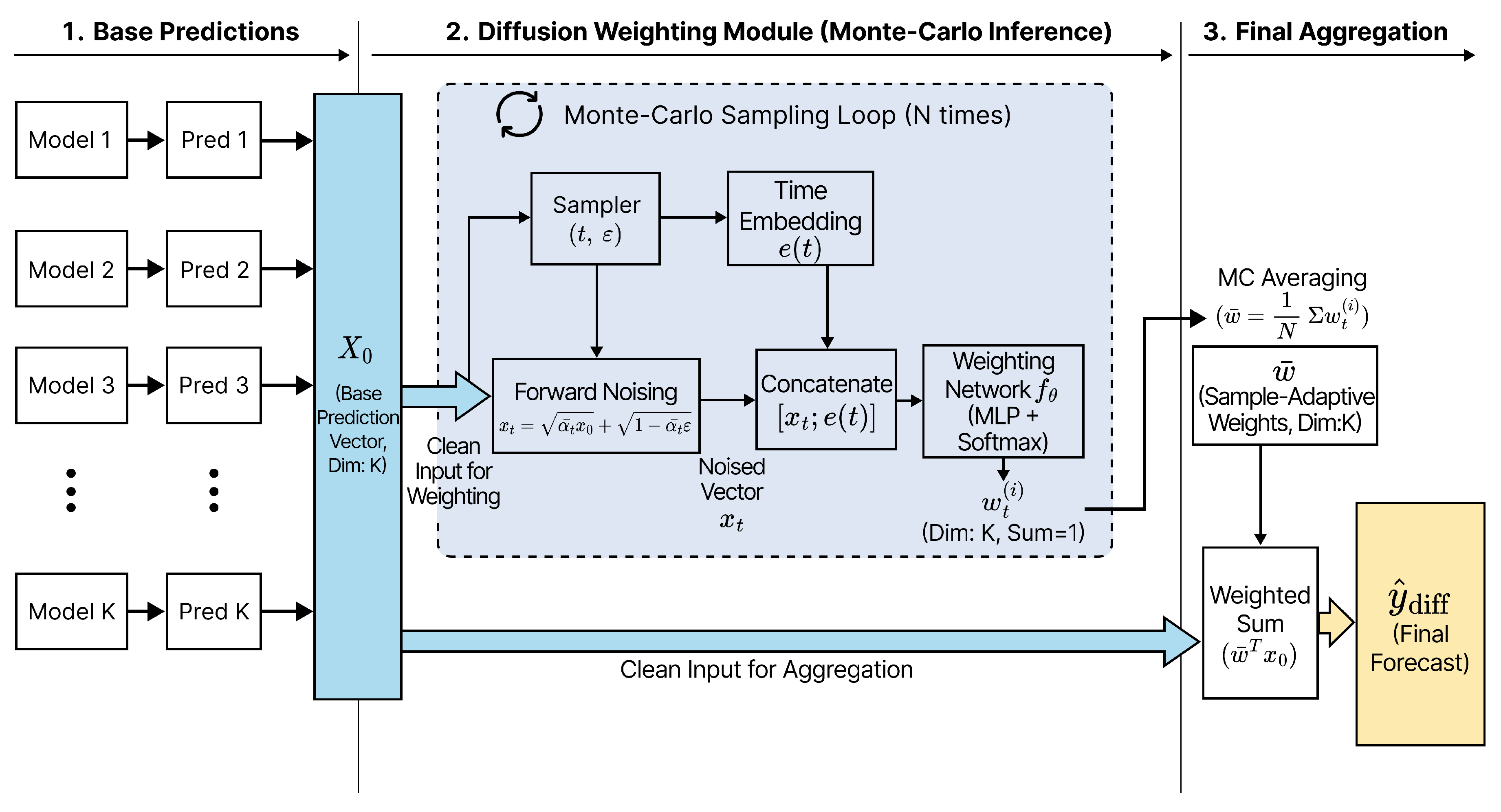
i.e., the weights are conditioned on the noised input but applied to the clean predictions . We train on the meta-train split while freezing all base models by minimizing the expected mean squared error under randomly sampled :
where the expectation is approximated by mini-batch sampling during training. At inference, we perform Monte-Carlo averaging by drawing M pairs , averaging the resulting weights , and applying the averaged weights to to obtain . Unless stated otherwise, we use a linear noise schedule from to over diffusion steps. The weighting network is implemented as a two-layer MLP with sinusoidal timestep embeddings (embedding dimension , hidden dimension 64) and is trained using AdamW (learning rate , weight decay ) for 20 epochs with gradient clipping at 1.0; at inference, we use Monte-Carlo draws.
4.6. Relation to Standard Diffusion Models
Standard diffusion generative models learn a reverse-time process to synthesize samples [32]. In contrast, our approach uses only forward noising and noise-conditioning to compute ensemble weights, avoiding iterative reverse sampling. Therefore, advances that accelerate reverse sampling (e.g., EDM, DPM-Solver, Consistency Models, and flow-based reformulations) are orthogonal to our objective [33,34,35,36]. Based on the methodology described above, we now evaluate the proposed ensemble strategies on the held-out test set. We compare the performance of individual base forecasters and different ensemble aggregation rules, with particular emphasis on the proposed diffusion-weighted ensemble. All reported results are obtained using the fixed experimental protocol and evaluation metrics described in this section.
5. Results
We evaluate forecasting performance using root-mean-square error (RMSE), mean absolute error (MAE), and the coefficient of determination (). All metrics are reported on the held-out test split unless stated otherwise. For interpretability, we report RMSE both in standardized anomaly units (after z-score normalization) and in physical units (°C) by converting predictions back using the training-set statistics.
5.1. Single-Model Performance
Table 3 compares the performance of individual forecasting models, including four DL forecasters (DLinear, iTransformer, PatchTST, LSTM) and two classical machine-learning baselines (LinearSVR and RF). Overall, the best single model achieves the lowest RMSE and MAE and the highest , indicating stronger agreement with the observed SST anomaly variability. We observe that the classical baselines remain competitive under the short-horizon setting (), suggesting that flattened lag features can still provide strong predictive signals for near-term SST anomalies.
Among individual forecasters, LSTM achieves the strongest overall accuracy, yielding the lowest test RMSE (0.3612 °C) and MAE (0.2627 °C) and the highest (0.6874) in Table 3. This suggests that, under the short-horizon setting (), recurrent modeling of local temporal dynamics remains effective for SST anomaly prediction. Notably, the classical baselines (LinearSVR and RF) remain competitive despite using flattened lag features, indicating that near-term SST anomalies contain strong linear and low-order nonlinear signals that can be exploited without explicit sequence modeling.
5.2. Ensemble Performance by Aggregation Rule
We compare three aggregation rules: uniform mean, validation-optimized convex weights, and the proposed diffusion-weighted ensemble. As shown in Table 4, uniform averaging provides a competitive but not consistently superior baseline, whereas validation-optimized convex weighting and the proposed diffusion-weighted ensemble improve upon the best single model.
Relative to the best single model (LSTM), the diffusion-weighted ensemble reduces the test RMSE from 0.3612 °C to 0.3595 °C, corresponding to a relative improvement of approximately 1.26%. A similar improvement is observed in MAE (from 0.2627 °C to 0.2619 °C; ∼0.305%), while increases from 0.6874 to 0.6902. Overall, these results indicate that aggregation primarily reduces variance and improves goodness-of-fit without sacrificing bias.
Uniform mean aggregation offers a stable baseline but cannot explicitly account for correlated forecast errors among base models. Validation-optimized convex weighting improves upon simple averaging by learning a global linear pool under nonnegativity and sum-to-one constraints. The proposed diffusion-weighted ensemble further improves performance by producing sample-adaptive mixture weights, providing a principled mechanism to vary weights across different conditions while consistently surpassing simpler pooling strategies.
5.3. Latitude-Band Error Analysis
To examine where the proposed ensemble improves the most, we compute test RMSE within 10° latitude bands and report band-wise errors for LSTM and the diffusion-weighted ensemble. This analysis highlights regional differences in predictability and helps interpret whether improvements are concentrated in specific latitude regimes.
Figure 4 and Table 5 show that the impact of diffusion-weighted ensembles is latitude-dependent. Notably, larger gains appear in several mid-to-high latitude bands (e.g., around 40°–60°), which often exhibit higher variance and more complex dynamics, while some low-latitude bands show marginal or negative changes. These results suggest that sample-adaptive weighting is particularly beneficial under regimes with stronger variability, supporting the use of adaptive ensembles for robust global SST forecasting. Explanation is that mid-to-high latitudes exhibit stronger variance and regime shifts, which amplify inter-model disagreement and nonstationary error correlations, making sample-adaptive weighting more beneficial. In contrast, tropical regions are often dominated by smoother variability, where base predictors tend to be more concordant and adaptive reweighting yields limited gains.
5.4. Best Subset Selection: Validation vs. Test
To study whether all four models are necessary, we evaluate all non-empty subsets of under each aggregation rule using the meta-train/meta-validation protocol described in Section 4.4. We consider three aggregation rules: uniform mean, validation-optimized convex weights, and the proposed diffusion-weighted ensemble. We report (i) the configuration selected by the lowest validation RMSE (the proper selection criterion) and (ii) the configuration that achieves the lowest test RMSE (reported only as a post hoc reference). Table 6 summarizes both cases.
The Val-best row in Table 6 represents the only configuration that is valid under our experimental protocol because it is selected using validation RMSE without accessing test labels. In contrast, the Test-best (post hoc) row is reported solely as a reference point and should not be interpreted as a deployable selection since it implicitly uses test outcomes for model selection. Importantly, the validation-selected diffusion configuration remains highly competitive on the test set (0.3597 °C), with only a negligible gap compared to the post hoc best-test configuration (0.3592 °C). This small difference suggests that validation-driven subset selection provides a reliable proxy for generalization and that the proposed diffusion-weighted ensemble remains effective even when the ensemble is formed from a reduced subset of base forecasters.
6. Conclusions and Discussions
In this study, we investigated short-horizon sea surface temperature (SST) forecasting from GODAS reanalysis using a diffusion-weighted ensemble framework. We constructed a multivariate global dataset from GODAS and defined SST as the near-surface (uppermost-level) potential temperature, with anomalies computed using training-period monthly climatology to reduce the dominant seasonal cycle. Under a controlled protocol with a fixed input window () and one-step forecasting horizon (), we trained heterogeneous base forecasters (DLinear, iTransformer, PatchTST, and LSTM) and generated out-of-sample predictions for validation and test splits to enable leak-free ensemble construction.
To combine base forecasts, we compared three aggregation rules with increasing modeling capacity: uniform mean, validation-optimized convex weighting (linear pool), and the proposed diffusion-weighted ensemble. Ensemble configuration selection was performed strictly within validation using a meta-train/meta-validation split, and the test set was used only once for final reporting. Overall, the results demonstrate that combining heterogeneous deep-learning forecasters improves robustness compared to the best single model, and that the diffusion-weighted ensemble consistently outperforms simpler global pooling strategies. Moreover, the latitude band analysis suggests that the benefits of sample-adaptive weighting are not uniform across regions; improvements are more pronounced in several mid-to-high latitude bands, while some low-latitude bands show marginal or negative changes. Finally, subset enumeration indicates that competitive performance can be achieved with reduced ensembles (e.g., three-model subsets), implying that strong performance does not necessarily require all candidate models when selection is conducted properly on validation.
Despite these promising results, several limitations remain. First, our experiments focus on a single short-horizon setting () and monthly GODAS data; extending the framework to longer lead times and higher temporal resolution (e.g., weekly or daily products) is required to fully characterize the advantages of diffusion-based adaptive aggregation under increased uncertainty. Second, GODAS is a reanalysis product and therefore reflects model and assimilation biases; evaluating the proposed ensemble on independent observational datasets and alternative reanalyses would strengthen the generality of the conclusions. Third, while we analyzed latitude-dependent errors, additional diagnostics (e.g., seasonality, regional ocean basins, and extreme-event regimes such as marine heatwaves) would provide deeper insight into when and why sample-adaptive weighting is most beneficial.
Future work will extend the proposed framework in three directions. (i) We will evaluate multi-step forecasting horizons and probabilistic calibration, including uncertainty-aware metrics, to quantify whether diffusion-weighted aggregation improves reliability as lead time increases. (ii) We will incorporate additional physically relevant predictors and alternative anomaly definitions to assess the sensitivity of model performance to preprocessing choices. (iii) We will explore lightweight and computationally efficient variants of the weighting network to enable deployment-oriented inference while preserving the benefits of sample-adaptive mixture weights. Collectively, this work demonstrates that diffusion-weighted, sample-adaptive aggregation provides a practical and effective pathway to improving the robustness of SST forecasting from multivariate global reanalysis data.
Data Availability Statement
The data used in this study are derived from public domain resources. The Global Ocean Data Assimilation System (GODAS) reanalysis data are publicly available from the NOAA National Centers for Environmental Information (NCEI) at https://psl.noaa.gov.
Acknowledgments
This work was supported by the Regional Innovation System & Education(RISE) program through the Chungnam RISE center, funded by the Ministry of Education(MOE) and the Chungcheongnam-do, Republic of Korea (2025-RISE-12-003).
Appendix A. Complete Results
This appendix provides full validation/test results to ensure transparency and reproducibility. All ensemble configurations are selected using validation only (meta-train/meta-validation protocol; Section 4.4), and the test split is used once for final reporting. We additionally report a test-oracle configuration solely as a post hoc reference to illustrate the upper bound.
Appendix A.1. Single-Model Baselines
Table A1 compares all single models on validation and test splits using RMSE, MAE, and . For the deep-learning models, we report both standardized metrics (z-score space) and physical-unit errors in °C (after inverse standardization). Classical baselines (LinearSVR, RF) are evaluated in standardized space. Note that RMSE/MAE in °C are obtained by inverse-transforming standardized predictions using training-set statistics, whereas z-space metrics directly reflect errors in normalized anomaly units.

Table A1.
Single-model performance on the validation and test splits.
| Model | Val RMSE (z) | Test RMSE (z) | Test MAE (z) | Test | Test RMSE (°C) | Test MAE (°C) |
|---|---|---|---|---|---|---|
| DLinear | 0.6331 | 0.6478 | 0.4746 | 0.6622 | 0.375 | 0.275 |
| iTransformer | 0.6303 | 0.6472 | 0.4757 | 0.6628 | 0.375 | 0.276 |
| PatchTST | 0.6254 | 0.6449 | 0.4715 | 0.6652 | 0.374 | 0.273 |
| LSTM | 0.6156 | 0.6231 | 0.4533 | 0.6874 | 0.361 | 0.263 |
| LinearSVR | 0.6248 | 0.6421 | 0.4684 | 0.6648 | 0.372 | 0.271 |
| RF | 0.6188 | 0.6398 | 0.4616 | 0.6672 | 0.370 | 0.267 |
For deep-learning models, we additionally report errors in physical units (SST in °C) after inverse standardization. For classical baselines (LinearSVR, RF), only standardized metrics are available.
Model shorthand (Appendix): D = DLinear, I = iTransformer, P = PatchTST, L = LSTM.
Appendix A.2. Best Ensemble Configurations
We report (i) the best ensemble configuration selected using validation RMSE (leak-free selection) and its corresponding test performance (Table A2), and (ii) the oracle best configuration by test RMSE for reference (Table A3). All configurations are selected from the candidate set that includes only the following aggregation rules: uniform mean (mean), validation-optimized convex weights (cw), and the proposed diffusion-weighted ensemble (diff). The “validation-selected” configuration is the only deployable choice under a proper generalization protocol. The “oracle” configuration is included for comparison only and must not be interpreted as a valid selection rule.
Table A2.
Best ensemble configuration selected by validation RMSE (standardized).
| Subset | K | Rule | Val RMSE (z) | Test RMSE (z) | Test | Test RMSE (°C) |
|---|---|---|---|---|---|---|
| I+P+L | 3 | diff | 0.6121 | 0.6206 | 0.6899 | 0.3597 |
This follows the leak-free protocol: we select the subset+aggregation rule using validation only, then report the corresponding test performance once.
Table A3.
Oracle best ensemble configuration by test RMSE (standardized).
| Subset | K | Rule | Val RMSE (z) | Test RMSE (z) | Test | Test RMSE (°C) |
|---|---|---|---|---|---|---|
| D+L | 2 | diff | 0.6140 | 0.6197 | 0.6909 | 0.3592 |
Shown for reference only. Selecting a configuration by test performance is not permitted for proper generalization evaluation.
Appendix A.3. All Subset and Aggregation Combinations
Table A4 provides the complete set of results for all evaluated subset and aggregation-rule combinations. Table A4 enumerates all non-empty subsets of and all aggregation rules (uniform mean/convex weights/diffusion-weighted). This complete listing enables direct comparison between subset choice and aggregation strategy under the same evaluation pipeline.
Table A4.
Complete results for all subset and aggregation-rule combinations (deep-learning ensembles only).
Table A4.
Complete results for all subset and aggregation-rule combinations (deep-learning ensembles only).
| Subset | K | Rule | Val RMSE (z) | Val MAE (z) | Val | Test RMSE (z) | Test MAE (z) | Test | Test RMSE (°C) |
|---|---|---|---|---|---|---|---|---|---|
| D | 1 | single | 0.6331 | 0.4510 | 0.6469 | 0.6478 | 0.4746 | 0.6622 | 0.375 |
| L | 1 | single | 0.6156 | 0.4406 | 0.6662 | 0.6231 | 0.4533 | 0.6874 | 0.361 |
| P | 1 | single | 0.6254 | 0.4475 | 0.6554 | 0.6449 | 0.4715 | 0.6652 | 0.374 |
| I | 1 | single | 0.6303 | 0.4505 | 0.6500 | 0.6472 | 0.4757 | 0.6628 | 0.375 |
| D+L | 2 | cw | 0.6141 | 0.4382 | 0.6678 | 0.6205 | 0.4518 | 0.6900 | 0.360 |
| D+L | 2 | diff | 0.6140 | 0.4383 | 0.6679 | 0.6197 | 0.4513 | 0.6909 | 0.359 |
| D+L | 2 | mean | 0.6166 | 0.4391 | 0.6650 | 0.6238 | 0.4553 | 0.6867 | 0.362 |
| D+P | 2 | cw | 0.6230 | 0.4448 | 0.6581 | 0.6407 | 0.4687 | 0.6696 | 0.371 |
| D+P | 2 | diff | 0.6227 | 0.4451 | 0.6584 | 0.6414 | 0.4692 | 0.6688 | 0.372 |
| D+P | 2 | mean | 0.6236 | 0.4449 | 0.6574 | 0.6404 | 0.4687 | 0.6699 | 0.371 |
| D+I | 2 | cw | 0.6255 | 0.4459 | 0.6553 | 0.6407 | 0.4701 | 0.6695 | 0.371 |
| D+I | 2 | diff | 0.6254 | 0.4455 | 0.6555 | 0.6390 | 0.4688 | 0.6713 | 0.370 |
| D+I | 2 | mean | 0.6254 | 0.4455 | 0.6555 | 0.6404 | 0.4696 | 0.6699 | 0.371 |
| P+L | 2 | cw | 0.6128 | 0.4374 | 0.6693 | 0.6215 | 0.4522 | 0.6890 | 0.360 |
| P+L | 2 | diff | 0.6126 | 0.4373 | 0.6694 | 0.6210 | 0.4520 | 0.6896 | 0.360 |
| P+L | 2 | mean | 0.6136 | 0.4379 | 0.6683 | 0.6244 | 0.4549 | 0.6862 | 0.362 |
| I+L | 2 | cw | 0.6130 | 0.4366 | 0.6690 | 0.6211 | 0.4523 | 0.6895 | 0.360 |
| I+L | 2 | diff | 0.6128 | 0.4365 | 0.6692 | 0.6204 | 0.4519 | 0.6901 | 0.360 |
| I+L | 2 | mean | 0.6145 | 0.4375 | 0.6673 | 0.6240 | 0.4553 | 0.6866 | 0.362 |
| I+P | 2 | cw | 0.6206 | 0.4428 | 0.6607 | 0.6377 | 0.4668 | 0.6727 | 0.370 |
| I+P | 2 | diff | 0.6203 | 0.4426 | 0.6610 | 0.6373 | 0.4666 | 0.6730 | 0.369 |
| I+P | 2 | mean | 0.6207 | 0.4428 | 0.6607 | 0.6377 | 0.4668 | 0.6726 | 0.370 |
| D+P+L | 3 | cw | 0.6127 | 0.4372 | 0.6693 | 0.6212 | 0.4520 | 0.6894 | 0.360 |
| D+P+L | 3 | diff | 0.6126 | 0.4372 | 0.6694 | 0.6207 | 0.4521 | 0.6898 | 0.360 |
| D+P+L | 3 | mean | 0.6157 | 0.4386 | 0.6660 | 0.6265 | 0.4573 | 0.6840 | 0.363 |
| D+I+L | 3 | cw | 0.6130 | 0.4366 | 0.6690 | 0.6210 | 0.4523 | 0.6895 | 0.360 |
| D+I+L | 3 | diff | 0.6127 | 0.4364 | 0.6693 | 0.6200 | 0.4518 | 0.6906 | 0.359 |
| D+I+L | 3 | mean | 0.6164 | 0.4384 | 0.6654 | 0.6261 | 0.4575 | 0.6845 | 0.363 |
| D+I+P | 3 | cw | 0.6205 | 0.4424 | 0.6609 | 0.6372 | 0.4664 | 0.6732 | 0.369 |
| D+I+P | 3 | diff | 0.6203 | 0.4423 | 0.6611 | 0.6369 | 0.4662 | 0.6735 | 0.369 |
| D+I+P | 3 | mean | 0.6211 | 0.4426 | 0.6602 | 0.6371 | 0.4665 | 0.6733 | 0.369 |
| I+P+L | 3 | cw | 0.6122 | 0.4360 | 0.6698 | 0.6209 | 0.4521 | 0.6896 | 0.360 |
| I+P+L | 3 | diff | 0.6121 | 0.4359 | 0.6699 | 0.6206 | 0.4523 | 0.6899 | 0.360 |
| I+P+L | 3 | mean | 0.6138 | 0.4370 | 0.6682 | 0.6254 | 0.4564 | 0.6851 | 0.362 |
| D+I+P+L | 4 | cw | 0.6122 | 0.4360 | 0.6698 | 0.6209 | 0.4521 | 0.6896 | 0.360 |
| D+I+P+L | 4 | diff | 0.6122 | 0.4359 | 0.6699 | 0.6203 | 0.4520 | 0.6902 | 0.360 |
| D+I+P+L | 4 | mean | 0.6155 | 0.4380 | 0.6662 | 0.6273 | 0.4583 | 0.6833 | 0.364 |
Rule abbreviations: single = base model; mean = uniform mean; cw = convex weights; diff = diffusion-weighted ensemble.
References
- Deser, C.; Alexander, M.A.; Xie, S.P.; Phillips, A.S. Sea surface temperature variability: Patterns and mechanisms. Annual review of marine science 2010, 2, 115–143. [CrossRef]
- Storto, A.; Alvera-Azcárate, A.; Balmaseda, M.A.; Barth, A.; Chevallier, M.; Counillon, F.; Domingues, C.M.; Drevillon, M.; Drillet, Y.; Forget, G.; et al. Ocean reanalyses: recent advances and unsolved challenges. Frontiers in Marine Science 2019, 6, 418. [CrossRef]
- Sun, D.; Li, F.; Jing, Z.; Hu, S.; Zhang, B. Frequent marine heatwaves hidden below the surface of the global ocean. Nature Geoscience 2023, 16, 1099–1104. [CrossRef]
- Storto, A.; Alvera-Azcárate, A.; Balmaseda, M.A.; Barth, A.; Chevallier, M.; Counillon, F.; Domingues, C.M.; Drevillon, M.; Drillet, Y.; Forget, G.; et al. Ocean reanalyses: recent advances and unsolved challenges. Frontiers in Marine Science 2019, 6, 418. [CrossRef]
- Ham, Y.G.; Kim, J.H.; Luo, J.J. Deep learning for multi-year ENSO forecasts. Nature 2019, 573, 568–572. [CrossRef]
- Montero-Manso, P.; Hyndman, R.J. Principles and algorithms for forecasting groups of time series: Locality and globality. International Journal of Forecasting 2021, 37, 1632–1653. [CrossRef]
- Wen, Q.; Zhou, T.; Zhang, C.; Chen, W.; Ma, Z.; Yan, J.; Sun, L. Transformers in time series: A survey. arXiv preprint arXiv:2202.07125 2022.
- De León Pérez, D.; Salazar-Galán, S.; Francés, F. Beyond Deterministic Forecasts: A Scoping Review of Probabilistic Uncertainty Quantification in Short-to-Seasonal Hydrological Prediction. Water 2025, 17, 2932. [CrossRef]
- Ehmimed, N.; Chkouri, M.Y.; Touhafi, A. Reliable and Adaptive Probabilistic Forecasting for Event-Driven Water-Quality Time Series Using a Gated Hybrid–Mixture Density Network. Sensors (Basel, Switzerland) 2025, 25, 7560. [CrossRef]
- Li, L.; Carver, R.; Lopez-Gomez, I.; Sha, F.; Anderson, J. Generative emulation of weather forecast ensembles with diffusion models. Science Advances 2024, 10, eadk4489. [CrossRef]
- Chen, F.; Gao, L. Learning Residual Distributions with Diffusion Models for Probabilistic Wind Power Forecasting. Energies 2025, 18, 4226. [CrossRef]
- Su, C.; Cai, Z.; Tian, Y.; Chang, Z.; Zheng, Z.; Song, Y. Diffusion models for time series forecasting: A survey. arXiv preprint arXiv:2507.14507 2025. [CrossRef]
- Barreto, F.T.; Curbani, F.E.; Zielinsky, G.M.; da Silva, M.B.; Lacerda, K.C.; Rodrigues, D.F. Development of a multigrid operational forecast system for the oceanic region off Rio de Janeiro State. Ocean Modelling 2023, 184, 102206.
- Storto, A.; Frolov, S.; Slivinski, L.; Yang, C. Correction of sea surface biases in the NEMO ocean general circulation model using neural networks. Geoscientific Model Development 2025, 18, 4789–4804. [CrossRef]
- Kong, W.; Lam, C.c.; Lau, D.s.; Chow, C.k.; Chong, S.n.; Chan, P.w.; Leung, N.c. Model validation and applications of wave and current forecasts from the Hong Kong Observatory’s Operational Marine Forecasting System. Ocean Modelling 2024, 190, 102393. [CrossRef]
- de Boisséson, E.; Balmaseda, M.A. Predictability of marine heatwaves: assessment based on the ECMWF seasonal forecast system. Ocean Science 2024, 20, 265–278. [CrossRef]
- Koul, V.; Brune, S.; Akimova, A.; Düsterhus, A.; Pieper, P.; Hövel, L.; Parekh, A.; Schrum, C.; Baehr, J. Seasonal prediction of Arabian Sea marine heatwaves. Geophysical Research Letters 2023, 50, e2023GL103975. [CrossRef]
- Hao, P.; Li, S.; Song, J.; Gao, Y. Prediction of sea surface temperature in the South China Sea based on deep learning. Remote Sensing 2023, 15, 1656. [CrossRef]
- Xu, T.; Zhou, Z.; Li, Y.; Wang, C.; Liu, Y.; Rong, T. Short-term prediction of global sea surface temperature using deep learning networks. Journal of Marine Science and Engineering 2023, 11, 1352. ttps://doi.org/10.3390/jmse11071352.
- Zrira, N.; Kamal-Idrissi, A.; Farssi, R.; Khan, H.A. Time series prediction of sea surface temperature based on BiLSTM model with attention mechanism. Journal of Sea Research 2024, 198, 102472. [CrossRef]
- Shi, B.; Ge, C.; Lin, H.; Xu, Y.; Tan, Q.; Peng, Y.; He, H. Sea surface temperature prediction using convlstm-based model with deformable attention. Remote Sensing 2024, 16, 4126. [CrossRef]
- Fu, Y.; Song, J.; Guo, J.; Fu, Y.; Cai, Y. Prediction and analysis of sea surface temperature based on LSTM-transformer model. Regional Studies in Marine Science 2024, 78, 103726. [CrossRef]
- Yang, Y.; Lam, K.M.; Dong, J.; Ju, Y. Multi-Factor Deep Learning Model for Sea Surface Temperature Forecasting. Remote Sensing 2025, 17, 752. [CrossRef]
- Dai, H.; Lei, F.; Wei, G.; Zhang, X.; Lin, R.; Zhang, W.; Shang, S. Sea surface temperature prediction by stacked generalization ensemble of deep learning. Deep Sea Research Part I: Oceanographic Research Papers 2024, 209, 104343. [CrossRef]
- Qian, J.; Wang, Q.; Liang, P.; Peng, S.; Wang, H.; Wu, Y. Deep learning–based ensemble forecast and predictability analysis of the Kuroshio intrusion into the south China sea. Journal of Physical Oceanography 2024, 54, 1503–1517. [CrossRef]
- Bonino, G.; Galimberti, G.; Masina, S.; McAdam, R.; Clementi, E. Machine learning methods to predict sea surface temperature and marine heatwave occurrence: a case study of the Mediterranean Sea. Ocean Science 2024, 20, 417–432. [CrossRef]
- Boschetti, F.; Feng, M.; Hartog, J.R.; Hobday, A.J.; Zhang, X. Sea surface temperature predictability assessment with an ensemble machine learning method using climate model simulations. Deep Sea Research Part II: Topical Studies in Oceanography 2023, 210, 105308. [CrossRef]
- Behringer, D.W.; Ji, M.; Leetmaa, A. An improved coupled model for ENSO prediction and implications for ocean initialization. Part I: The ocean data assimilation system. Monthly Weather Review 1998, 126, 1013–1021. [CrossRef]
- Breiman, L. Random Forests. Machine Learning 2001, 45, 5–32. [CrossRef]
- Smola, A.J.; Schölkopf, B. A tutorial on support vector regression. Statistics and Computing 2004, 14, 199–222. [CrossRef]
- Akiba, T.; Sano, S.; Yanase, T.; Ohta, T.; Koyama, M. Optuna: A Next-generation Hyperparameter Optimization Framework. In Proceedings of the Proceedings of the 25th ACM SIGKDD International Conference on Knowledge Discovery & Data Mining (KDD ’19). ACM, 2019, pp. 2623–2631. [CrossRef]
- Ho, J.; Jain, A.; Abbeel, P. Denoising Diffusion Probabilistic Models. arXiv preprint arXiv:2006.11239 2020.
- Karras, T.; Aittala, M.; Aila, T.; Laine, S. Elucidating the Design Space of Diffusion-Based Generative Models. In Proceedings of the Advances in Neural Information Processing Systems (NeurIPS), 2022.
- Lu, C.; Zhou, Y.; Bao, F.; Chen, J.; Li, C.; Zhu, J. DPM-Solver: A Fast ODE Solver for Diffusion Probabilistic Model Sampling in Around 10 Steps. In Proceedings of the Advances in Neural Information Processing Systems (NeurIPS), 2022.
- Song, Y.; Dhariwal, P.; Chen, M.; Sutskever, I. Consistency Models. In Proceedings of the International Conference on Machine Learning (ICML), 2023.
- Liu, X.; Gong, C.; Liu, Q. Flow Straight and Fast: Learning to Generate and Transfer Data with Rectified Flow. arXiv preprint arXiv:2209.03003 2022.
Figure 1.
Global map of near-surface potential temperature from GODAS
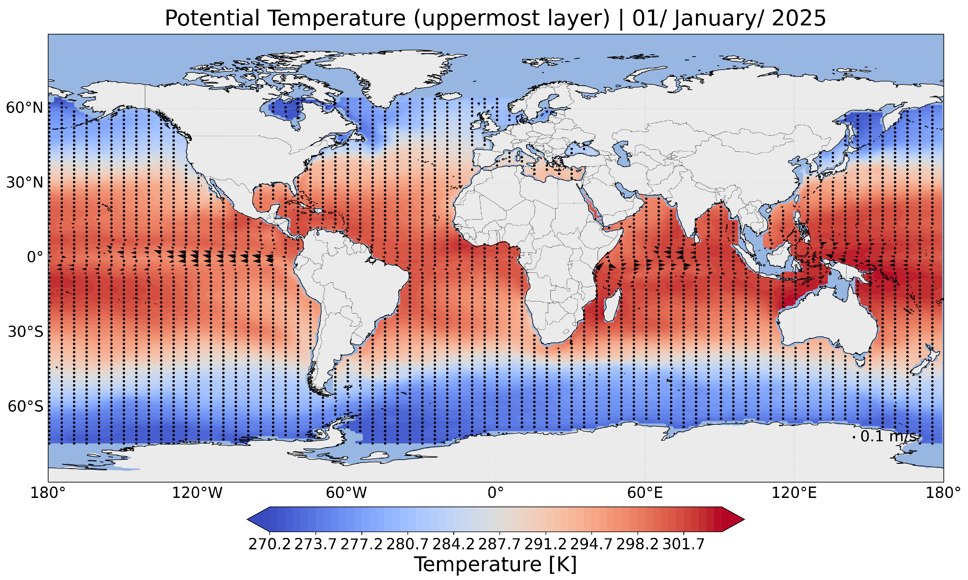
Figure 4.
Test RMSE by latitude band (10° bins). The diffusion-weighted ensemble is compared against the best single model (LSTM) to reveal latitude-dependent performance differences.
Figure 4.
Test RMSE by latitude band (10° bins). The diffusion-weighted ensemble is compared against the best single model (LSTM) to reveal latitude-dependent performance differences.
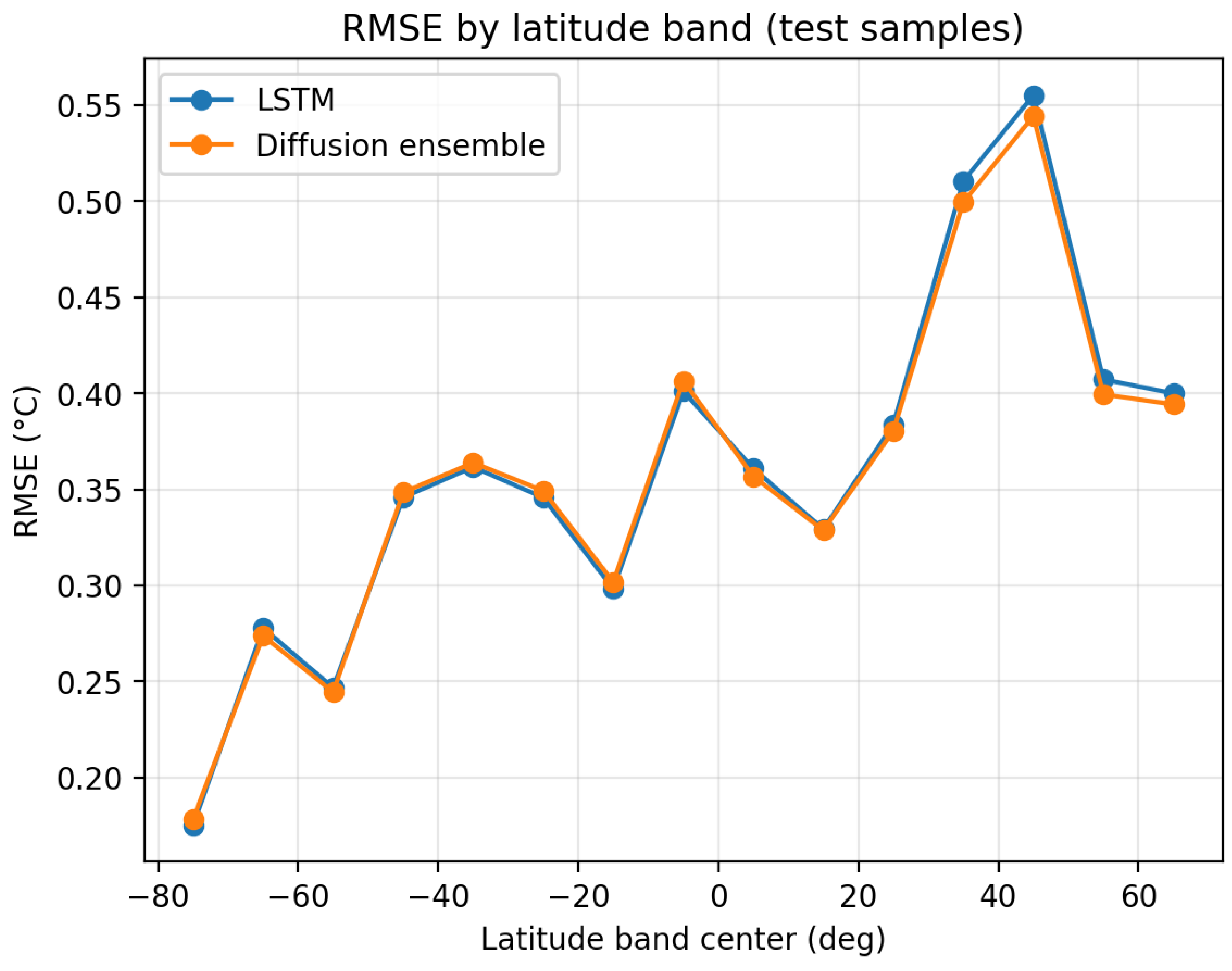
Table 1.
All oceanographic variables are provided by the GODAS reanalysis dataset.
| Category | Variable | Description |
|---|---|---|
| Temperature | Potential temperature | Ocean potential temperature is provided at multiple vertical levels |
| Salinity | Salinity | Ocean salinity field provided at multiple vertical levels |
| Ocean currents | U of current | Zonal (east-west) component of ocean current velocity |
| V of current | Meridional (north–south) component of ocean current velocity | |
| Vertical motion | Geometric vertical velocity | Vertical velocity component of ocean flow |
| Sea level | Sea surface height relative to geoid | Sea surface height referenced to the geoid |
| Vertical structure | Ocean mixed layer depth below sea surface | Depth of the surface ocean mixed layer |
| Ocean isothermal layer depth below sea surface | Depth of the isothermal layer below the sea surface | |
| Surface forcing | Total downward heat flux at surface | Net downward heat flux at the ocean surface |
| Zonal momentum flux | Zonal component of surface momentum flux | |
| Meridional momentum flux | Meridional component of surface momentum flux | |
| Salt flux | Surface salt flux at the ocean–atmosphere interface |
Table 2.
Oceanographic variables selected from the GODAS dataset and used in this study.
| Category | Variable | Description |
|---|---|---|
| Temperature | Potential temperature (uppermost level) | Near-surface ocean potential temperature used as a proxy for sea surface temperature |
| Ocean currents | U of current | Zonal (east-west) component of ocean current velocity |
| V of current | Meridional (north-south) component of ocean current velocity | |
| Vertical structure | Ocean mixed layer depth below sea surface | Depth of the surface ocean mixed layer |
| Ocean isothermal layer depth below sea surface | Depth of the isothermal layer below the sea surface | |
| Sea level | Sea surface height relative to geoid | Sea surface height referenced to the geoid |
| Surface forcing | Total downward heat flux at the surface | Net downward heat flux at the ocean surface |
Table 3.
Test performance of individual forecasting models. RMSE is reported in standardized units (std) and in physical units (°C). Best values (lowest error / highest ) are highlighted in bold.
Table 3.
Test performance of individual forecasting models. RMSE is reported in standardized units (std) and in physical units (°C). Best values (lowest error / highest ) are highlighted in bold.
| Model | RMSE (std) | RMSE (°C) | MAE (°C) | |
|---|---|---|---|---|
| DLinear | 0.6478 | 0.3755 | 0.2751 | 0.6622 |
| iTransformer | 0.6472 | 0.3751 | 0.2731 | 0.6628 |
| PatchTST | 0.6449 | 0.3738 | 0.2733 | 0.6652 |
| LSTM | 0.6231 | 0.3612 | 0.2627 | 0.6874 |
| LinearSVR | 0.6420 | 0.3720 | 0.2683 | 0.6648 |
| RF | 0.6400 | 0.3710 | 0.2620 | 0.6672 |
Table 4.
Test performance of ensemble methods using all four deep models. Best values are highlighted in bold.
Table 4.
Test performance of ensemble methods using all four deep models. Best values are highlighted in bold.
| Method | RMSE (std) | RMSE (°C) | MAE (°C) | |
| Single (LSTM) | 0.6231 | 0.3612 | 0.2627 | 0.6874 |
| Ensemble — Mean | 0.6273 | 0.3636 | 0.2656 | 0.6833 |
| Ensemble — Convex Weight | 0.6209 | 0.3599 | 0.2620 | 0.6896 |
| Ensemble — Diffusion-weighted | 0.6203 | 0.3595 | 0.2619 | 0.6902 |
Table 5.
Band-wise test RMSE by latitude. denotes the relative difference of the Diffusion-weighted ensemble over LSTM: . we use half-open intervals [a,b)
Table 5.
Band-wise test RMSE by latitude. denotes the relative difference of the Diffusion-weighted ensemble over LSTM: . we use half-open intervals [a,b)
| Lat. center | Range | N | RMSE (LSTM) | RMSE (Diff) | Imp (%) |
|---|---|---|---|---|---|
| -70 | [-75,-65) | 3482 | 0.2362 | 0.2328 | 1.4609 |
| -60 | [-65,-55) | 6252 | 0.2688 | 0.2656 | 1.1991 |
| -50 | [-55,-45) | 6325 | 0.2798 | 0.2798 | -0.0173 |
| -40 | [-45,-35) | 5814 | 0.3711 | 0.3747 | -0.9910 |
| -30 | [-35,-25) | 5113 | 0.3599 | 0.3629 | -0.8338 |
| -20 | [-25,-15) | 4900 | 0.3173 | 0.3204 | -1.0026 |
| -10 | [-15,-5) | 4654 | 0.3322 | 0.3385 | -1.8934 |
| 0 | [-5,5) | 4739 | 0.4028 | 0.4016 | 0.2937 |
| 10 | [5,15) | 4752 | 0.3475 | 0.3470 | 0.1289 |
| 20 | [15,25) | 4136 | 0.3291 | 0.3272 | 0.5689 |
| 30 | [25,35) | 3661 | 0.4301 | 0.4252 | 1.1389 |
| 40 | [35,45) | 3143 | 0.5953 | 0.5807 | 2.4479 |
| 50 | [45,55) | 2594 | 0.4352 | 0.4274 | 1.7936 |
| 60 | [55,65) | 1861 | 0.4105 | 0.4030 | 1.8258 |
Table 6.
Best ensemble configurations. The left row is selected by the lowest validation RMSE (proper selection). The right row shows the post hoc best test RMSE (for reference). Here, D = DLinear, I = iTransformer, P = PatchTST, and L = LSTM.
Table 6.
Best ensemble configurations. The left row is selected by the lowest validation RMSE (proper selection). The right row shows the post hoc best test RMSE (for reference). Here, D = DLinear, I = iTransformer, P = PatchTST, and L = LSTM.
| Selection | Subset + Aggregation | Val RMSE (°C) | Test RMSE (°C) | Test MAE (°C) | Test |
|---|---|---|---|---|---|
| Val-best | I + P + L; Diffusion | 0.3548 | 0.3597 | 0.2621 | 0.6899 |
| Test-best (post hoc) | D + L; Diffusion | 0.3559 | 0.3592 | 0.2616 | 0.6909 |
Disclaimer/Publisher’s Note: The statements, opinions and data contained in all publications are solely those of the individual author(s) and contributor(s) and not of MDPI and/or the editor(s). MDPI and/or the editor(s) disclaim responsibility for any injury to people or property resulting from any ideas, methods, instructions or products referred to in the content. |
© 2026 by the authors. Licensee MDPI, Basel, Switzerland. This article is an open access article distributed under the terms and conditions of the Creative Commons Attribution (CC BY) license (http://creativecommons.org/licenses/by/4.0/).
Copyright: This open access article is published under a Creative Commons CC BY 4.0 license, which permit the free download, distribution, and reuse, provided that the author and preprint are cited in any reuse.


