
Submitted:
18 September 2025
Posted:
21 September 2025
You are already at the latest version
Abstract
At NOAA/NWS/National Centers for Environmental Prediction (NCEP), a global ensemble forecast system based on GraphCast—a machine-learning weather model developed by Google DeepMind—has been tested. This study compares the machine-learning-based global ensemble forecast system (MLGEFS) with the NCEP operational physics-based global ensemble forecast system (GEFS). The goal is not to determine which system performs better or worse, but rather to understand the similarities and differences between them. We aim to gain insights into how to improve or better design AI models, particularly ensemble prediction systems based on AI, as well as AI-driven forecast post-processing, product generation, and verification methods. To capture both warm and cold season dynamics, one winter case and one summer case were carefully examined across various aspects of ensemble performance. Three similarities—forecast accuracy, ensemble spread, and inter-variable correlation—and four differences—ensemble-averaging effectiveness, nonlinearity, chaos, and blurriness—were identified. Additionally, one assessment of forecast information was conducted. As a side result (the “fifth difference”), the less uniform performance of ensemble members observed in MLGEFS compared to GEFS, may indicate that ensemble post-processing could be more important in AI-based ensemble systems than in physics-based NWP ensembles. Given the early exploratory stage of AI-based weather forecasting, this study may raise more questions than it answers, which is expected to stimulate further research in this emerging field.
Keywords:
Google DeepMind
; GraphCast weather model
; global ensemble forecast system (GEFS)
; AI model
; physical model
1. Introduction
To address the chaotic nature of the atmospheric system (Lorenz, 1963 [1]), ensemble forecasting has been widely adopted in modern numerical weather prediction (NWP) systems around the world (Buizza et al., 2018 [2]; Du et al., 2018 [3]). An ensemble prediction system (EPS) generates multiple plausible forecasts—known as “ensemble members”—simultaneously, allowing for a quantitative estimation of forecast uncertainty and the predictability of future weather events. Running a model multiple times with slightly varied initial conditions and physical configurations is computationally expensive. Meteorologists must carefully balance ensemble size (i.e., the number of members) and model spatial resolution to optimize the use of computational resources (e.g., Du et al., 1997 [4]; Clark et al., 2011 [5]).
In recent years, machine learning (ML) and artificial intelligence (AI)-based data-driven weather forecasting models have emerged rapidly (e.g., Pathak et al., 2022 [6]; Lam et al., 2023 [7]; Bi et al., 2023 [8]; Lang et al., 2024 [9]; Chen et al., 2024 [10]). These AI techniques offer the potential for breakthroughs in weather forecasting (Ebert-Uphoff and Hilburn, 2023 [11]). One major advantage of AI-based models is their ability to run significantly faster and with far fewer computational resources once trained—making them particularly well-suited for ensemble forecasting such as GenCast (Price et. al., [12]), ECMWF’s AIFS ensemble (Lang et al., 2024 [9]), and FGN (Flexible Generative Network, Alet et al., 2025 [13]).
However, data-driven AI-model or machine-learning-based weather prediction (MLWP) is still in its infancy, and many aspects of model performance remain poorly understood. As a result, the meteorological community is calling for comprehensive comparisons between MLWP and traditional physics-based NWP systems to advance scientific understanding (Radford et al., 2024 [14]). This study is one such response to that call (e.g., Bouallegue et al., 2024 [15]; Charlton-Perez et al., 2024 [16]; DeMaria, 2024 [17]).
At NOAA/NWS/NCEP (National Oceanic and Atmospheric Administration/National Weather Service/National Centers for Environmental Prediction), the machine-learning global forecast system (MLGFS) and the machine-learning global ensemble forecast system (MLGEFS) have been tested (Wang et al., 2024 [18]; Wang et al., 2025 [19]), both based on the GraphCast model developed by Google DeepMind (Lam et al., 2023 [7]). To mirror the configuration of the NCEP operational Global Ensemble Forecast System (GEFS), MLGEFS includes 31 ensemble members—matching the number used in GEFS. Readers are referred to Section 2 for further details about the models.
This study compares various aspects of ensemble performance between MLGEFS and GEFS. The objective is not to determine which system performs better or worse, but rather to examine their similarities and differences and understand the underlying reasons. Through this comparison, we aim to gain insights into how to improve or better design AI models—particularly AI-model-based ensemble prediction systems (AI-EPS)—as well as AI-based forecast products, post-processing techniques, and verification methods.
Given the early exploratory stage of AI-based weather forecasting, this study may raise more questions than it answers, which is expected to stimulate further research in the field.
2. Model and Data
2.1. MLGEFS
The MLGEFS is built upon the foundational architecture of GraphCast (Lam et al., 2023 [7]). GraphCast is a neural network model based on graph neural networks (GNNs), structured in an encode–process–decode configuration (Battaglia et al., 2018 [20]). With 36.7 million parameters, GraphCast enables high-resolution global weather prediction by leveraging a multi-mesh representation of Earth’s surface. GraphCast is available in two versions. The first version supports 37 pressure levels and was trained on ECMWF’s ERA5 reanalysis data from 1979 to 2017 (Hersbach et al., 2020 [21]). The second version includes 13 pressure levels and was fine-tuned by DeepMind using ECMWF’s HRES analysis data from 2016 to 2021, in addition to the original ERA5 training. The second version is used in our MLGEFS experiments. A detailed description of the GraphCast architecture is provided in the companion paper (Wang et al., 2025 [19]).
By utilizing diverse data sources, perturbation techniques, and a multi-step fine-tuning schedule, MLGEFS was constructed (Wang et al., 2025 [19]). Multiple data sources—including the NCEP in-house Global Forecast System (GFS) data assimilation system (GDAS), ECMWF’s ERA5 reanalysis, and operational HRES analysis—were used to fine-tune GraphCast. During model training, input states (i.e., initial conditions or ICs) were derived from GDAS data spanning March 20, 2021, to January 1, 2023. The dataset was split into training and validation subsets: training data covered March 20, 2021, to September 1, 2022, while validation data spanned September 1, 2022, to January 1, 2023. Based on earlier test results showing that IC-only perturbation produced insufficient ensemble spread, both model and data uncertainties were incorporated into MLGEFS—referred to as the “Mixed” approach in Wang et al. (2025 [19]). During fine-tuning, 30 distinct model weights were generated as “model perturbations” (effectively representing multiple versions of the model). In parallel, 30 perturbed ICs from GEFS.v12.0 were used to account for IC uncertainty. Each perturbed IC was paired with a corresponding model weight, resulting in 30 ensemble members. Additionally, one control member was run using GraphCast with the standard model weight and an unperturbed (control) GEFS IC. Thus, a total of 31 MLGEFS members were produced—matching the ensemble size of GEFS (see next subsection). This ensemble approach generated 16-day forecasts at a horizontal resolution of 0.25 degrees (approximately 25 km grid spacing).
2.2. GEFS
The counterpart physics-based ensemble prediction system used for comparison with MLGEFS is the NCEP Global Ensemble Forecast System (GEFS). GEFS is based on the NCEP Global Forecast System (GFS), which utilizes the FV3 dynamical core (Lin et al., 2017 [22]). The most current operational version is GEFS version 12 (Zhou et al., 2022 [23]; Fu et al., 2024 [24]). GEFS consists of 31 members—one unperturbed control member and 30 perturbed members—at approximately 25-km horizontal resolution (0.25 degrees). It runs four forecast cycles per day at 00, 06, 12, and 18 UTC, with a forecast length of up to 35 days (840 hours), producing output every six hours. Initial condition perturbations are generated using an Ensemble Kalman Filter (EnKF)-based data assimilation system (Kleist and Ide, 2015 [25]). The control analysis is identical to the initial conditions used in the deterministic GFS model. In addition to IC perturbations, GEFS incorporates stochastic physics schemes to account for model uncertainty.
2.3. Data and Study Cases
To examine regional-scale weather systems in greater detail, verification was conducted over the Continental United States (CONUS) domain. Analyses from the GFS data assimilation system (GDAS) were used as the reference truth. To capture both warm- and cold-season conditions, one winter case (initialized at 00Z on February 27, 2024) and one summer case (initialized at 00Z on July 1, 2024) were selected. The case selection was entirely random and not tailored to any specific flow regime; they were simply drawn from test cases provided by the AI/ML group. Each test case includes a 16-day forecast with 6-hourly outputs from both MLGEFS and GEFS.
3. Comparison of MLGEFS and GEFS
3.1. Similarities
3.1.1. Forecast Accuracy
Figure 1 compares the root-mean-squared error (RMSE) of 2-meter surface air temperature (T2m) and 500-hPa geopotential height (500H) forecasts between MLGEFS (blue curves) and GEFS (red curves) for both the winter (upper panel) and summer (lower panel) cases. The two systems exhibit very similar temporal evolution, showing parallel trends throughout the 16-day forecast period. Comparable parallel-trend behavior is also observed in their biases (Figure 2), even when the biases differ in sign (e.g., Figure 2c). Overall, their performance is similar, with each system occasionally outperforming or underperforming the other. This closely aligned behavior raises an important question: Why do they perform so similarly? Could it be that the AI model (GraphCast) has implicitly learned the physical principles of numerical weather prediction (NWP) through its pre-training on ERA5 reanalysis data? MLGEFS may have internalized physical relationships across various synoptic scenarios and now behaves similarly to a physics-based model. For example, Figure 3 shows that MLGEFS (left panel) exhibits atmospheric instabilities comparable to those in GEFS (right panel). In the winter case, both Figure 3a,b display a pronounced cold-front-like baroclinic instability zone along the trough at the 850-hPa level. In the summer case, Figure 3c,d reveal a convectively unstable region located in a weakly forced low-pressure area at the northwest edge of the subtropical high. This result supports the findings of Hakim and Masanam (2023) [26], who reported that AI models can realistically reproduce fundamental physical laws. Since both systems are initialized with the same initial conditions, it is worth considering how much of this similarity is attributable to that factor. This remains a topic for further discussion.
The atmospheric instabilities illustrated in Figure 3 are defined as follows. The baroclinic instability is represented by the magnitude of horizontal temperature gradient:
where is the change in temperature T (K) in the zonal (x) direction, is the change in temperature T (K) in the meridional (y) direction, and are the corresponding distances in kilometers. Baroclinicity is calculated at each isobaric level for each ensemble member. Then, the ensemble mean baroclinicity is computed across all members at each level and shown in Figure 3a–b.
The convective instability is calculated using Eq. (2):
where is the equivalent potential temperature. In a convectively unstable (stable) atmosphere, a rising air parcel will accelerate (decelerate) because it is warmer (cooler) than the surrounding environment. Convective instability is calculated for each member using data from the 1000–700 hPa layer (i.e., 1000, 950, 850, and 700 hPa levels), representing the lower portion of the atmosphere where convection typically occurs. Based on each member’s value, an ensemble mean of convective instability is computed and displayed in Figure 3c–d.
3.1.2. Ensemble Spread
Ensemble spread refers to the dispersion of ensemble members around their mean and is used to quantify forecast uncertainty or confidence. It is defined as the standard deviation of ensemble members relative to the ensemble mean. Figure 4 shows the domain-averaged ensemble spread of 2-meter surface air temperature (T2m) and 500-hPa geopotential height (500H) for both winter and summer cases from MLGEFS and GEFS. Similar to the behavior of a physics-based ensemble model (GEFS, red curves), the ensemble spread of MLGEFS (blue curves) generally increases over time. Specifically, in the winter case (Figure 4a,b), GEFS’s spread grows steadily throughout the forecast period, and MLGEFS exhibits a similar trend. In the summer case (Figure 4c,d), GEFS’s spread increases rapidly during the first week and then saturates; MLGEFS follows the same pattern. In terms of magnitude, MLGEFS’s spread is initially smaller, catches up around day 10, and exceeds GEFS’s spread after two weeks.
Regarding spatial structure, Figure 5 compares the 850-hPa spread (color shaded) for both winter (upper panel) and summer (lower panel) cases between MLGEFS (left) and GEFS (right). While the finer details differ, the large-scale patterns are generally similar and highly spatially correlated. The spread is larger in trough regions and smaller in ridge or high-pressure areas, which is meteorologically consistent. The average spatial correlation of the 850-hPa spread between MLGEFS and GEFS is approximately 0.8 for both winter and summer cases (Figure 6).
In a physical NWP model, ensemble spread growth or decay is typically associated with atmospheric instabilities—especially baroclinic instability in large-scale flows—although these relationships are not always straightforward. Why, then, does ensemble spread in an AI model grow in a similar manner to that in a physics-based model? To explore this, we examine whether the relationship between spread and instabilities in the AI model mirrors that of the physics-based model. Figure 7 compares the spatial correlation between ensemble spread and instability fields for T2m and 500H in both winter and summer cases from MLGEFS and GEFS. Overall, the correlation between spread and instabilities in the AI ensemble (MLGEFS) is indeed similar to that in the physics-based ensemble (GEFS), for both baroclinic (solid line) and convective (dashed line) instabilities. When a positive (negative) correlation is observed in GEFS, a similar correlation appears in MLGEFS. Their time-evolving trends are also generally aligned, with one notable exception: the relationship with baroclinic instability in the summer case (Figure 7d). In MLGEFS, the correlation increases after Day 4, whereas in GEFS, it decreases over time. This result further suggests that the AI model captures not only linear statistical properties but also retains internal physical relationships akin to those in NWP models—what we might call “learned physics.” However, these relationships may not always be identical, as illustrated in Figure 7d, which warrants further investigation.
Since ensemble spread is a measure of forecast uncertainty, the relationship between ensemble spread and forecast error—known as the “spread-error relation”—is a key indicator of ensemble quality. Given the previously noted similarities in both forecast performance (i.e., forecast error) and ensemble spread, the spread-error relation is also expected to be similar between MLGEFS and GEFS. The magnitude aspect of the spread-error relation is often quantified using the Consistency score, defined by Equation (3):
Here, RMSE represents the forecast error of the ensemble mean, and both RMSE and spread are domain-averaged values. This metric can be applied to any variable. A Consistency value of 1.0 indicates a perfect ensemble, where the RMSE equals the ensemble spread. Values greater than 1.0 suggest an under-dispersive ensemble (spread too small relative to error), while values less than 1.0 indicate an over-dispersive ensemble (spread larger than error).
Figure 8 compares the Consistency scores of MLGEFS and GEFS. Both systems exhibit similar behavior: under-dispersion prior to approximately Day 10, followed by near-perfect dispersion thereafter. The two peaks in MLGEFS around Day 7 (Figure 8a,b) are attributed to larger forecast errors, as seen in Figure 1a,b. The structural aspect of the spread-error relation is assessed via the spatial correlation between two-dimensional spread and absolute forecast error fields, shown in Figure 9 for T2m and 500H in both winter and summer cases. Both MLGEFS and GEFS show positive correlations, indicating that ensemble spread is a reasonably good predictor of potential forecast errors in both systems. Although the spread-error relation is generally stronger for GEFS than for MLGEFS prior to Day 10—due to the smaller spread in MLGEFS as shown in Figure 4—MLGEFS still demonstrates a similarly useful spread-error relationship, comparable to that of a physics-based model.
3.1.3. Inter-Variable Correlation
In a physics-based NWP model, all model-produced variables are physically coupled and interconnected, as they are governed by the model’s equations and physical laws. But is this inter-variable connection still preserved in an AI model? Some researchers argue that it is not (e.g., Bonavita, 2024 [27]), while others suggest otherwise (e.g., Hakim and Masanam, 2023 [26]). We examine this question in our MLGEFS forecast experiments from two perspectives: one based on a single forecast (“solo” setting, Figure 10), and the other based on ensemble performance (“group” setting, Figure 11 and Figure 12). Figure 10 shows the spatial correlation between different variables—T2m and SLP (blue), and 500H and 850T (red)—from the control forecasts of MLGEFS (solid line) and GEFS (dashed line) for both winter (Figure 10a) and summer (Figure 10b) cases. The inter-variable correlations of the MLGEFS control member closely follow those of the GEFS control forecast across various scenarios: strongly positively coupled periods (e.g., 500H–850T in both winter and summer, Figure 10a,b), strongly negatively coupled periods (e.g., T2m–SLP in summer, Figure 10b), and weakly coupled or variable periods with alternating positive, negative, or uncoupled relationships (e.g., T2m–SLP in winter, Figure 10a).
Figure 11 shows an example (Day 7) of the Performance Rank Histogram (also called the Equal-Likelihood Histogram), which displays the percentage chance of each ensemble member being closest to the truth (i.e., the analysis) for three variables—T2m, H500, and SLP—in both winter (upper panel) and summer (lower panel) cases. Results are shown for MLGEFS (left panel) and GEFS (right panel), calculated over all grid points within the verification domain. In a physics-based ensemble model, the performance of ensemble members across different variables is often interrelated. For example, if one variable performs better (or worse), another strongly coupled variable is likely to perform similarly (as seen in Figure 10). In other words, the relative performance histograms (such as those in Figure 11) for different variables should generally be positively correlated. However, if two variables are weakly coupled or uncoupled (as also seen in Figure 10a), their relative performance histograms may show little or even negative correlation. Figure 12 displays the correlation of relative performance histograms over the entire forecast period (Days 1–16) for two variable pairs: T2m–500H (left panel) and 500H–SLP (right panel), in both winter and summer cases. As expected, a general positive correlation is observed for GEFS—and notably, this is also true for MLGEFS. Although the details do not match exactly, the overall trends are similar: when the relative performances of variables are positively, negatively, or not correlated in GEFS, the same pattern is observed in MLGEFS. Thus, both the single forecast analysis (Figure 10) and the ensemble group forecast evaluation (Figure 12) suggest that inter-variable correlation is similarly preserved in the AI-based MLGEFS as in the physics-based GEFS.
From the relative performance histogram in Figure 11, we observe another notable phenomenon: the distribution of bars is less uniform for MLGEFS than for GEFS. A few members—such as member #2 in Figure 11a and member #8 in Figure 11c—consistently outperform the others in MLGEFS, appearing as the best-performing member far more frequently. This suggests that ensemble post-processing may play a more important role in AI-based ensemble systems than in physics-based NWP ensembles. Why is the variation in performance among members greater in MLGEFS than in GEFS? One possible explanation is that the relative performance ranking of ensemble members exhibits less variation in MLGEFS compared to GEFS. This hypothesis will be discussed further in Section 3.2.2.
3.2. Differences
3.2.1. Effectiveness of Ensemble Averaging
In a well-designed ensemble system, averaging across many members can effectively filter out non-predictable features, resulting in an ensemble mean forecast that is superior to the control forecast (i.e., the original deterministic forecast without running an ensemble). Therefore, the degree of improvement—often measured by error reduction—of the ensemble mean over the control forecast can serve as an indicator of the effectiveness of the ensemble technique. Figure 13 compares the forecast error (absolute error, |forecast − analysis|) reduction percentage of the ensemble mean relative to the control member for T2m and 500H in both winter and summer cases, for MLGEFS and GEFS. Overall, ensemble averaging is more effective in GEFS (the red curve), yielding greater error reduction than in MLGEFS (the blue curve). Except for the first 2–3 days, the ensemble mean of GEFS consistently shows lower error than its control forecast, whereas this is not always the case for MLGEFS. On many days, the ensemble mean in MLGEFS is either similar to or worse than the control forecast. For GEFS, the improvement generally increases with forecast lead time, while this trend is less apparent in MLGEFS. Why is that? One possible explanation may lie in differences in nonlinearity between the two systems (see Section 3.2.2).
3.2.2. Nonlinearity
Since initial condition perturbations are added around the unperturbed control analysis, the perturbed members would evolve symmetrically around the control member over time if the forecast system were quasi-linear (Figure 14b). In such cases, the ensemble mean would remain close to the control member. In contrast, if the forecast system is strongly nonlinear, both perturbed and unperturbed members evolve asymmetrically over time, resulting in the control member diverging significantly from the ensemble mean (Figure 14a). Therefore, the difference between the control member and the ensemble mean forecast—normalized by the ensemble spread—can be used as a measure of the system’s nonlinearity (Du and Zhou, 2011 [28]):
Equation (4) can be applied to any variable of interest. Figure 15 compares the nonlinearities of T2m and 500H in both winter and summer cases between MLGEFS and GEFS. As expected, nonlinearity is lower at the beginning and generally increases with forecast lead time in the physics-based ensemble GEFS (red curves). It also varies by regime, peaking around Days 12–13 before slightly decreasing. In contrast, nonlinearity in the AI-based ensemble MLGEFS (blue curves) remains nearly constant throughout the entire forecast period. As a result, MLGEFS exhibits higher nonlinearity than GEFS during the initial days, but this relationship reverses later in the forecast. This behavior may help explain why ensemble averaging is more effective during the first 2–3 days in MLGEFS but becomes less effective afterward, as observed in Figure 13.
3.2.3. Randomness or Chaos
Selz and Craig (2023) [29] suggested that AI models are less chaotic than physics-based models. To examine this in our ensemble model experiment, we apply the Performance Rank Variation Score (PRVS, proposed by Du, 2025 [30]). PRVS measures the variation—or randomness—of ensemble members’ relative performance ranks in space or time. A larger PRVS indicates more frequent flipping of performance ranks between two points, suggesting greater randomness or chaotic behavior among ensemble members; a smaller PRVS implies more consistent performance. Figure 16 compares the PRVS of T2m and 500H in both winter and summer cases between MLGEFS and GEFS at three forecast lead times (Days 1, 10, and 16). Since PRVS increases with the separation distance between two points before reaching saturation, an array of PRVS values across seven separation distances (~25, 50, 100, 200, 300, 400, and 500 km) is shown in Figure 16. The results show greater variability in GEFS (red curves) than in MLGEFS (blue curves) in most cases, suggesting that MLGEFS is less random or chaotic. However, the difference diminishes with increasing forecast lead time (as seen in Figure 16b,c), and may even reverse slightly at longer time ranges, such as the Day-16 result shown in Figure 16d.
How can this be explained? While the exact reason remains uncertain, one hypothesis is that reduced forecast error cascade effects in AI models—and the role of intrinsic atmospheric predictability—may contribute. Unlike physics-based NWP models, where forecast errors accumulate and cascade from smaller to larger scales during time-step integration, AI models directly predict the output at the next forecast time. This may result in fewer error cascades and a lower degree of performance variability among ensemble members in the short term. This property could also contribute to extended predictability in AI models, as reported by Vonich and Hakim (2025 [31]). At longer lead times, however, forecasts may approach the intrinsic atmospheric predictability limit, where ensemble behavior is governed more by the atmosphere itself than by model architecture—leading to similar levels of randomness across both AI and physics-based models. These are compelling questions for future research.
By comparing Figure 15 and Figure 16, an interesting and seemingly “contradictory” result emerges during the first few days of the forecast. Specifically, in MLGEFS, larger nonlinearity (Figure 15) corresponds to smaller variation in ensemble members’ relative performance ranks (Figure 16), while in GEFS, the opposite is observed—smaller nonlinearity corresponds to greater variation in performance ranks. A possible explanation for this apparent contradiction is that the relationship between nonlinearity and chaos may differ across forecasting systems such as MLGEFS and GEFS. The nature of the nonlinearity–chaos relationship in AI-based modeling systems could be a valuable topic for future research.
3.2.4. Blurriness
Figure 17 shows an example in which the MLGEFS forecast fields appear smoother or blurrier compared to their GEFS counterparts. To quantify this, we calculated the standard deviation (Equation 5) to measure the spatial variation of each of the 31 ensemble members’ forecasts over the verification domain for T2m and 500H in both winter and summer cases. The average result across all 31 members is shown in Figure 18 for MLGEFS (blue curves) and GEFS (red curves).
where is the value of a variable X of interest at grid point, is the domain-averaged value of X, and n is the total number of grid points within the verification domain. Figure 18 quantitatively confirms that the spatial variation in MLGEFS is smaller than that in GEFS throughout the entire forecast period (Days 1-16).
3.3. How Much Extra Information Provided by MLGEFS Beyond GEFS?
Does MLGEFS provide new information beyond what GEFS already offers? To address this question, we retrospectively derived the statistical best and worst members from the 31 ensemble members of each system (MLGEFS and GEFS) and compared their error bounds. Here’s how they were constructed: at each grid point, the member with the smallest absolute forecast error was selected. After applying this procedure across all grid points in the domain, a statistical best member was formed. In this composite member, the identity of the ensemble member may vary from one grid point to another. Similarly, a statistical worst member was derived by selecting the member with the largest absolute error at each grid point.
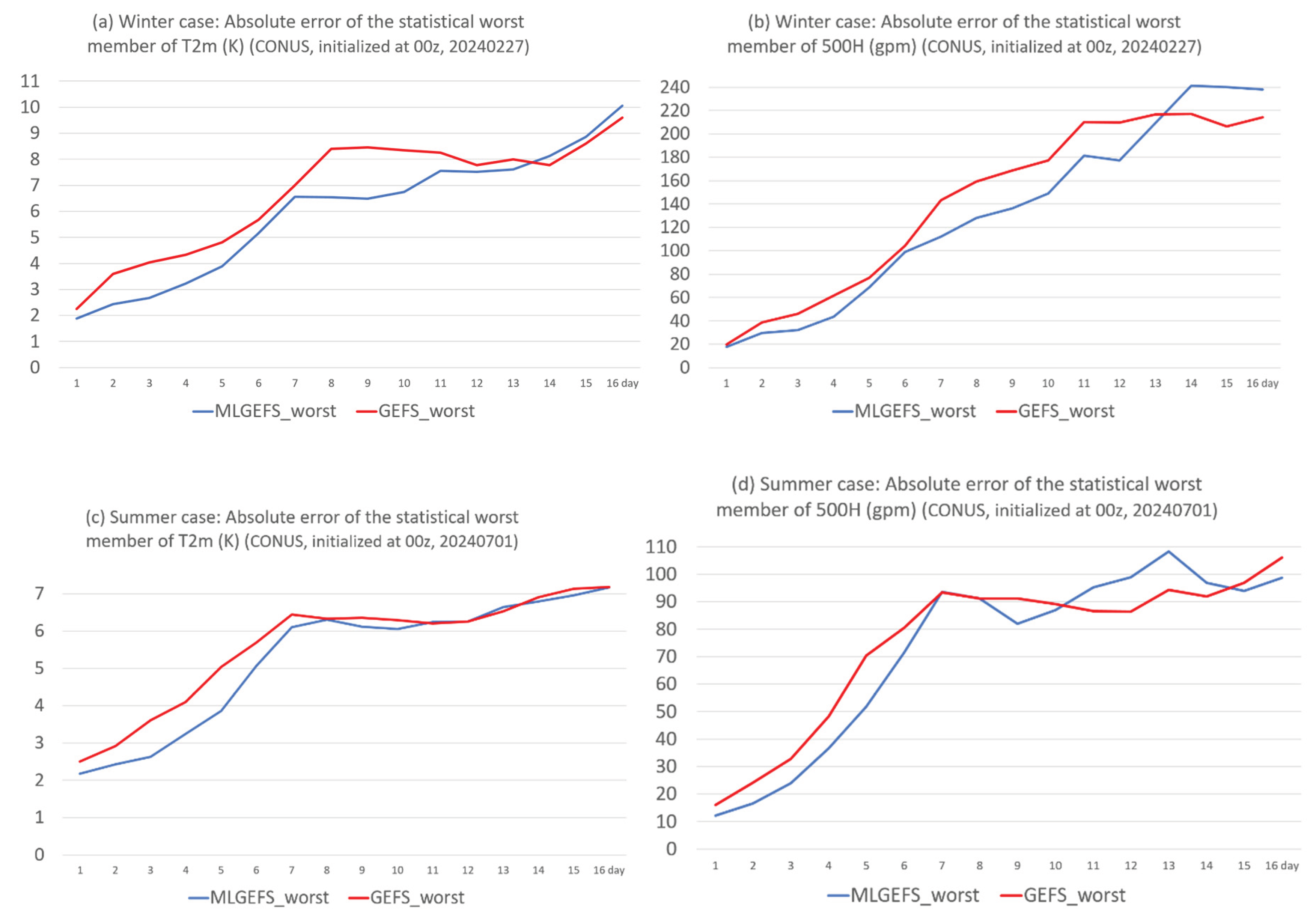
Figure 19 shows the absolute forecast errors of the best members for T2m and 500H in both winter and summer cases—representing the “lower bound of error.” Generally, MLGEFS errors (blue curves) are larger than or comparable to those of GEFS (red curves), except for a few forecast times (e.g., Days 8–9 in Figure 19c and Days 15–16 in Figure 19d). This suggests that MLGEFS generally does not provide better forecast information than GEFS, although it occasionally does. Figure 20 presents the same analysis but for the worst members—representing the “upper bound of error.” In contrast to the best-member results, MLGEFS errors are generally smaller than or comparable to those of GEFS, except for a few forecast times (e.g., Days 14–16 in Figure 20b and Days 11–13 in Figure 20d). This indicates that MLGEFS generally does not introduce worse forecast information than GEFS either.
In other words, the forecast information provided by GEFS largely encompasses what MLGEFS can offer in this experiment. One possible reason is that MLGEFS exhibits a smaller ensemble spread than GEFS prior to approximately Days 13–14 (as shown in Figure 4). Therefore, improving ensemble spread in the current version of MLGEFS is necessary to enhance the quality of forecast information—by increasing the likelihood of capturing better forecasts while minimizing the risk of introducing poorer ones. To achieve this, we plan to test a diffusion model–based MLGEFS (such as GenCast; Price et al., 2024 [12]) in future experiments.
4. Summary
By comparing various aspects of ensemble performance between the experimental AI-model-based MLWP ensemble (MLGEFS, built on GraphCast) and the NCEP operational physics-based NWP ensemble (GEFS) in both winter and summer cases, the following results are observed.
Three similarities:
- (1)
- In terms of forecast accuracy (error and bias), MLGEFS performs very similarly to the physics-based model GEFS, suggesting that the AI model may have implicitly learned the internal “physics” of NWP systems by memorizing physical relationships across various synoptic scenarios during its training period. MLGEFS also exhibits fundamental meteorological behaviors—such as baroclinic and convective instabilities—comparable to those seen in GEFS. To what extent is this similarity attributable to the shared initial conditions used by both models? This remains an open question for further discussion.
- (2)
- MLGEFS exhibits a smaller ensemble spread at the beginning but gradually catches up and even surpasses that of GEFS after two weeks. The growth trend and spatial structure of MLGEFS’s ensemble spread are similar—or parallel—to those of GEFS, which may be attributed to their comparable relationships between spread and atmospheric instabilities (baroclinic and convective). Although GEFS demonstrates a quantitatively stronger spread–error relationship, particularly in the early forecast period, MLGEFS closely mirrors this behavior and even outperforms GEFS at longer lead times.
- (3)
- The output variables from MLGEFS are interconnected in a manner similar to those in a physics-based model. This interconnection is observed in both single forecast settings and ensemble group forecast settings. It further suggests that the AI model may “understand” the physical relationships inherent in NWP models, rather than relying solely on linear statistical properties. A side result (the “fifth difference”) observed from the performance-rank histogram (Figure 11) is that ensemble members in MLGEFS exhibit less uniform performance compared to those in GEFS. This implies that ensemble post-processing may play a more important role in AI-based ensemble systems than in physics-based NWP ensembles.
Four differences:
- (4)
- One of the key advantages of running an ensemble weather forecast is the ability to filter out unpredictable features and improve the ensemble mean forecast through averaging across individual members. Although ensemble averaging is more effective in enhancing the ensemble mean forecast over the control forecast during the first few days, it is generally less effective in the AI-based ensemble MLGEFS compared to the physics-based ensemble GEFS. In MLGEFS, the ensemble mean forecast does not consistently outperform the control member, whereas in GEFS, it reliably does. This difference may be related to the nonlinearity characteristics of MLGEFS (see point (5) below).
- (5)
- Unlike in a physics-based model, where nonlinearity generally increases with forecast lead time and varies with flow regimes, nonlinearity in MLGEFS remains nearly constant throughout the ensemble forecast period (Days 1–16).
- (6)
- MLGEFS exhibits a less chaotic nature than GEFS, particularly at shorter forecast lead times. The spatial variation in ensemble members’ relative performance ranks—i.e., the frequency of rank changes or “flipping”—is lower in MLGEFS than in GEFS. This may result in less uniform performance among members, with a few consistently outperforming the others. Such behavior suggests that ensemble post-processing (forecast calibration) may be even more essential for AI-based ensembles than for physics-based NWP ensembles (also see the point (3) above). A question that arises from comparing points (5) and (6) is whether the relationship between nonlinearity and chaos differs across forecasting systems like MLGEFS and GEFS. This could be a valuable topic for future research.
- (7)
- The AI-based model MLGEFS tends to produce spatially smoother fields than the physics-based NWP model GEFS. To address this issue, improvements to the AI model architecture may be necessary—such as incorporating diffusion models—an area for AI scientists to explore further.
One assessment of forecast information:
- (8)
- Finally, by examining the forecast errors of both the best and worst members, we investigated whether the current version of MLGEFS introduces any new forecast information beyond what GEFS already provides. Our findings suggest that MLGEFS contributes little additional forecast information—either positive or negative—compared to GEFS. In other words, the forecast information from MLGEFS is largely encompassed by GEFS. The good news is that MLGEFS does not introduce unreliable or misleading outputs into the final forecast products, as some have feared. However, the downside is that its overall contribution remains limited. This outcome may be attributed to the smaller ensemble spread in the current version of MLGEFS. To enhance the value of MLGEFS, more sophisticated ensemble perturbation methods are needed—ones that can increase the diversity of useful forecast information while minimizing the risk of introducing poor-quality predictions. A diffusion-model-based approach, such as GenCast, could be a promising candidate for future testing. Several other strategies may be worth exploring: (a) Noise-aware training or ensemble learning with stochastic perturbations to better capture chaotic dynamics; (b) Training with regime-aware or physics-informed loss functions; (c) Replacing autoregressive rollouts with diffusion models or transformers; (d) Developing improved ensemble perturbation strategies Additionally, because AI models are significantly more computationally efficient than physics-based models, dramatically increasing ensemble size is feasible in AI-based ensemble prediction systems—offering another pathway to enhance forecast diversity and value (Mahesh et al., 2024 and 2025 [32,33]).
Given the early exploratory stage of AI model-based weather forecasting, we recognize that this study may raise more questions than it answers. We hope these new questions—and even moments of confusion—will inspire further research and curiosity among readers.
Data Availability Statement
The GEFS data can be downloaded from NCEP’s operational products inventory under Global Ensemble Forecast System at https://www.nco.ncep.noaa.gov/pmb/products/gens/. The MLGEFS experimental data is available upon request.
Acknowledgments
The authors want to thank Dr. Jacob Carley for his support of this work and Drs. Gwen Chen and Bo Yang for their initial reviewing the manuscript. The experimental run of the MLGEFS is supported by the Inflation Reduction Act and the NOAA Software Engineering for Novel Architectures (SENA) project. This research received no external funding.
References
- Lorenz, E.N. Deterministic nonperiodic flow. J. Atmos. Sci., 1963, 20, 130–141. [Google Scholar] [CrossRef]
- Buizza, R.; Du, J.; Toth, Z.; Hou, D. Major operational ensemble prediction systems (EPS) and the future of EPS. In the book of Handbook of Hydrometeorological Ensemble Forecasting (edited by Q. Duan et al.), 2018, Springer, Berlin, Heidelberg, pp1-43. [CrossRef]
- Du, J.; Berner, J.; Buizza, R.; Charron, M.; Houtekamer, P.; Hou, D.; Jankov, I.; Mu, M.; Wang, X.; Wei, W.; Yuan, H. Ensemble methods for meteorological predictions. In the book of Handbook of Hydrometeorological Ensemble Forecasting (edited by Q. Duan et al.), 2018, Springer, Berlin, Heidelberg, pp1-52. [CrossRef]
- Du, J.; Mullen, S. L. , and Sanders, F. Short-range ensemble forecasting of quantitative precipitation. Mon. Wea. Rev. 1997, 125, 2427–2459. [Google Scholar] [CrossRef]
- Clark, A.J.; Kain, J.S.; Stensrud, D.J.; Xue, M.; Kong, F.; Coniglio, M.C.; Thomas, K.W.; Wang, Y.; Brewster, K.; Gao, J.; Weiss, S.J.; Bright, D.; Du, J. Probabilistic precipitation forecast skill as a function of ensemble size and spatial scale in a convection-allowing ensemble, Mon. Wea. Rev. 2011, 139, 1410–1418. [Google Scholar] [CrossRef]
- Pathak, J. , and Coauthors. FourCastNet: A global data-driven high-resolution weather model using adaptive fourier neural operators. 2022, 2202.11214.
- Lam, R.; Sanchez-Gonzalez, A.; Willson, M.; Wirnsberger, P.; Fortunato, M.; Pritzel, A.; et al. Graphcast: Learning skillful medium-range global weather forecasting. Science 2023, 382, 1416–1421. [Google Scholar] [CrossRef] [PubMed]
- Bi, K.; Xie, L.; Zhang, H.; Chen, X.; Gu, X.; Tian, Q. Accurate medium range global weather forecasting with 3-D neural networks. Nature 2023, 1–6. [Google Scholar] [CrossRef]
- Lang, S., and Coauthors. AIFS—ECMWF’s data-driven forecasting system. 2024, URL https: //arxiv.org/abs/2406.01465, 2406.01465.
- Chen, L.; Zhong, X.; Li, H.; et al. A machine learning model that outperforms conventional global subseasonal forecast models. Nature Communications 2024, 15. [Google Scholar] [CrossRef]
- Ebert-Uphoff, I.; Hilburn, K. The outlook for AI weather prediction. Nature 2023, 619, 473–474. [Google Scholar] [CrossRef]
- Price, I. and co-authors. GenCast: Diffusion-based ensemble forecasting for medium-range weather. arXiv 2024, arXiv:2312.15796v2,. [CrossRef]
- Alet, F., Price, I., and El-Kadi A., & others. Skillful joint probabilistic weather forecasting from marginals. 2025. https://arxiv.org/abs/2506.10772.
- Radford, J. T., Ebert-Uphoff, I., DeMaria, R., Tourville, N., and Hilburn, K. Accelerating Community-Wide Evaluation of AI Models for Global Weather Prediction by Facilitating Access to Model Output. Bulletin of the American Meteorological Society 2024.
- Bouallegue, Z. B. , and Coauthors. The rise of data-driven weather forecasting: A first statistical assessment of machine learning–based weather forecasts in an operational-like context. Bulletin of the American Meteorological Society 2024, 105, E864–E883. [Google Scholar] [CrossRef]
- Charlton-Perez, A. J. , and Coauthors. Do AI models produce better weather forecasts than physics-based models? A quantitative evaluation case study of storm ciaran. NPJ Climate and Atmospheric Science 2024, 7, 93. [Google Scholar] [CrossRef]
- DeMaria, R. Evaluation of tropical cyclone track and intensity forecasts from purely ML-based weather prediction models, illustrated with FourCastNet. 2024, https: //ams.confex.com/ams/104ANNUAL/meetingapp.cgi/Paper/436711.
- Wang, J.; Tabas, S. S., Cui, L., Du, J., Fu, B., Yang, F., Levit, J., Stajner, I., Carley, J., Tallapragada, V., and Gross, B. Machine learning weather prediction model development for global ensemble forecasts at EMC. EGU24 AS5.5 -- Machine Learning and Other Novel Techniques in Atmospheric and Environmental Science: Application and Development. Vienna, Austria, April 18, 2024.
- Wang, J.; Tabas, S. S., Fu, B., Cui, L., Zhang, Z., Zhu, L., Peng, J., and Carley, J. 2025. Development of a hybrid ML and physical model global ensemble system. 2025, NCEP Office Note, No. 522, 23pp. [CrossRef]
- Battaglia, P.W. and co-authors. Relational inductive biases, deep learning, and graph networks. 2018, arXiv:1806.01261v3. [CrossRef]
- Hersbach, H. , Bell B., Berrisford, P, and coauthors. The ERA4 global reanalysis. QJRMS 2020, 146. [Google Scholar] [CrossRef]
- Lin, S. J. , Putman, W., and Harris, L. FV3: the GFDL finite-volume cubed-sphere dynamical core (Version 1), NWS/NCEP/EMC, 2017, https://www.gfdl.noaa.gov/wp-content/uploads/2020/02/FV3-Technical-Description.pdf.
- Zhou, X. , and Coauthors. The Development of the NCEP Global Ensemble Forecast System Version 12. Wea. and Forecasting 2022, 37, 1069–1084. [Google Scholar] [CrossRef]
- Fu, B.; Zhu, Y.; Guan, H.; Sinsky, E.; Yang, B.; Xue, X.; Pegion, P.; Yang, F. Weather to seasonal prediction from the UFS coupled Global Ensemble Forecast System. Weather and Forecasting 2024, 39. [Google Scholar] [CrossRef]
- Kleist, D. T. , and Ide, K. An OSSE-based evaluation of hybrid variational-ensemble data assimilation for the NCEP GFS, Part I: System description and 3D-hybrid results. Mon. Wea. Rev. 2015, 143, 433–451. [Google Scholar] [CrossRef]
- Hakim, G. J. , and Masanam, S. Dynamical Tests of a Deep Learning Weather Prediction Model. Artificial Intelligence for the Earth Systems 2024, 3. [Google Scholar] [CrossRef]
- Bonavita, M. . On some limitations of current machine learning weather prediction models. Geophysical Research Letters 2024, 51, e2023GL107377. [Google Scholar] [CrossRef]
- Du, J.; Zhou, B. A dynamical performance-ranking method for predicting individual ensemble member’s performance and its application to ensemble averaging. Mon. Wea. Rev. 2011, 129, 3284–3303. [Google Scholar]
- Selz, T.; Craig, G.C. Can artificial intelligence-based weather prediction models simulate the butterfly effect? Geophysical Research Letters 2023, 50, e2023GL105747. [Google Scholar] [CrossRef]
- Du, J. Performance Rank Variation Score (PRVS) to measure the variation in ensemble member’s relative performance with an introduction to “Transformed Ensemble” post-processing method. Meteorology 2025, 4, 20. [Google Scholar] [CrossRef]
- Vonich, P. T. , and Hakim, G. J. Testing the Limit of Atmospheric Predictability with a Machine Learning Weather Model. 2025. [CrossRef]
- Mahesh, A., Collins, W., Bonev, B., & co-authors. Huge Ensembles Part I: Design of Ensemble Weather Forecasts using Spherical Fourier Neural Operators. 2024. [CrossRef]
- Mahesh, A. , Collins, W., Boney, B., & co-authors. Huge Ensembles Part II: Properties of a Huge Ensemble of Hindcasts Generated with Spherical Fourier Neural Operators. 2025, https://arxiv.org/pdf/2408.01581.
Figure 1.
Root-mean-squared error (rmse, y-axis) of ensemble mean forecast for (a) T2m and (b) 500H from MLGEFS (blue) and GEFS (red), in the winter case (initialized from 00z, Feb. 27, 2024). The values are averaged over the CONUS domain. (c) and (d) are the same as (a) and (b) but for the summer case (initialized from 00z, July 1, 2024). All forecasts are projected into 16 days (384 hours). X-axis is the forecast time (in days).
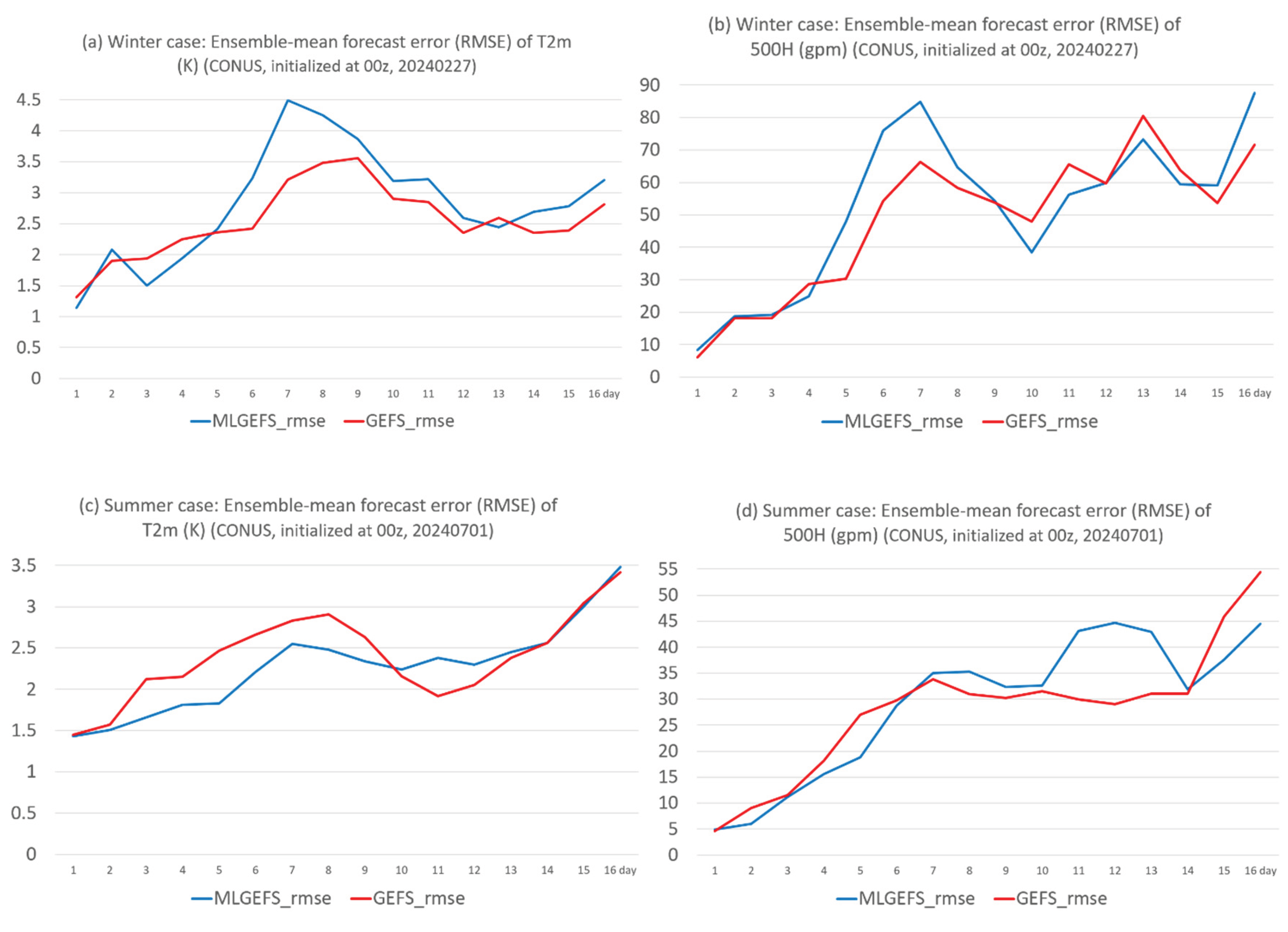
Figure 2.
Same as Figure 1 but for bias.
Figure 2.
Same as Figure 1 but for bias.
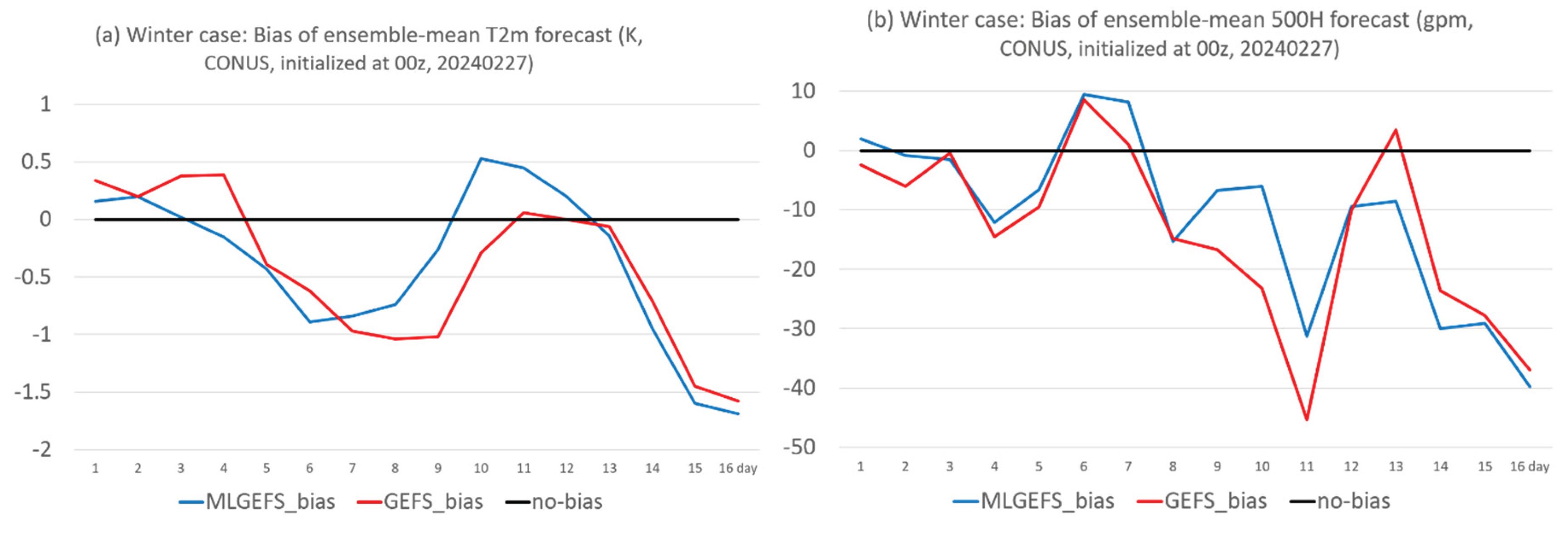
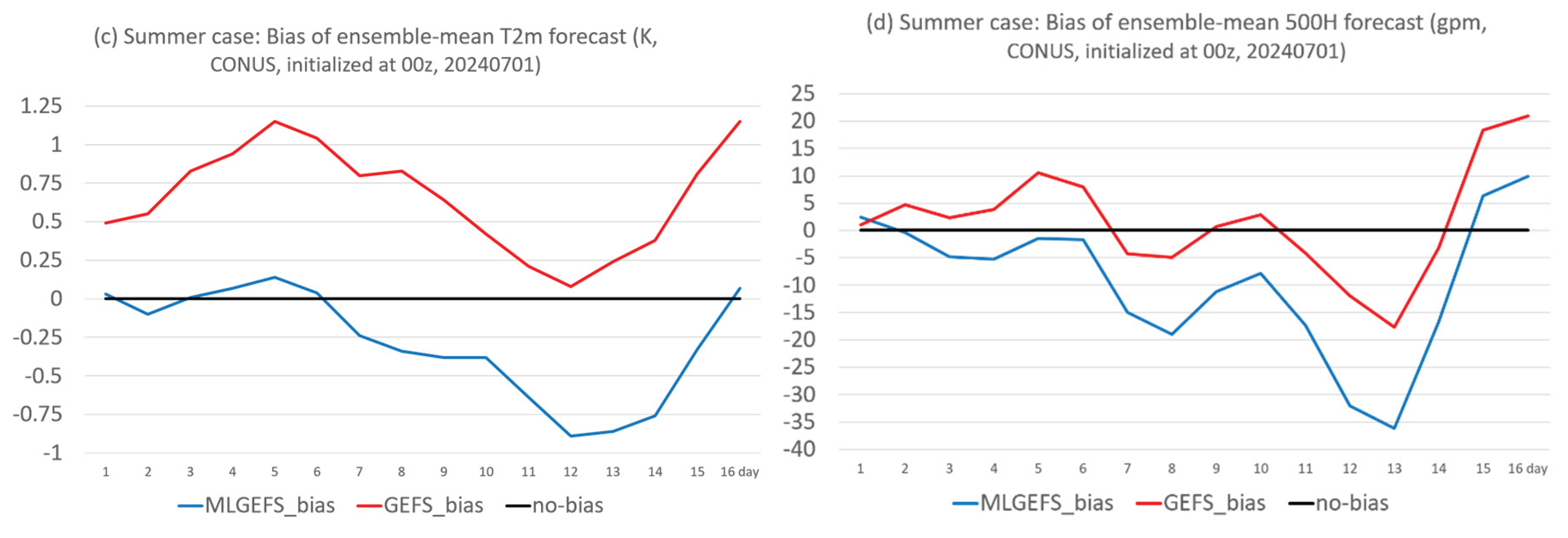
Figure 3.
(a) A winter example of baroclinic instability (color shaded, unit: K/km) from MLGEFS’s 24hr forecast of 850H (initialized from 00z, Feb. 27, 2024). The black contour is the ensemble spread, and the blue contour is the ensemble mean. (b) is the same as (a) but from GEFS. (c) A summer example of convective instability (color shaded, unit: K/hPa) from MLGEFS’s 240hr forecast of 850H (initialized from 00z, July 1, 2024). (d) is the same as (c) but from GEFS.
Figure 4.
Same as Figure 1 but for ensemble spread.
Figure 4.
Same as Figure 1 but for ensemble spread.
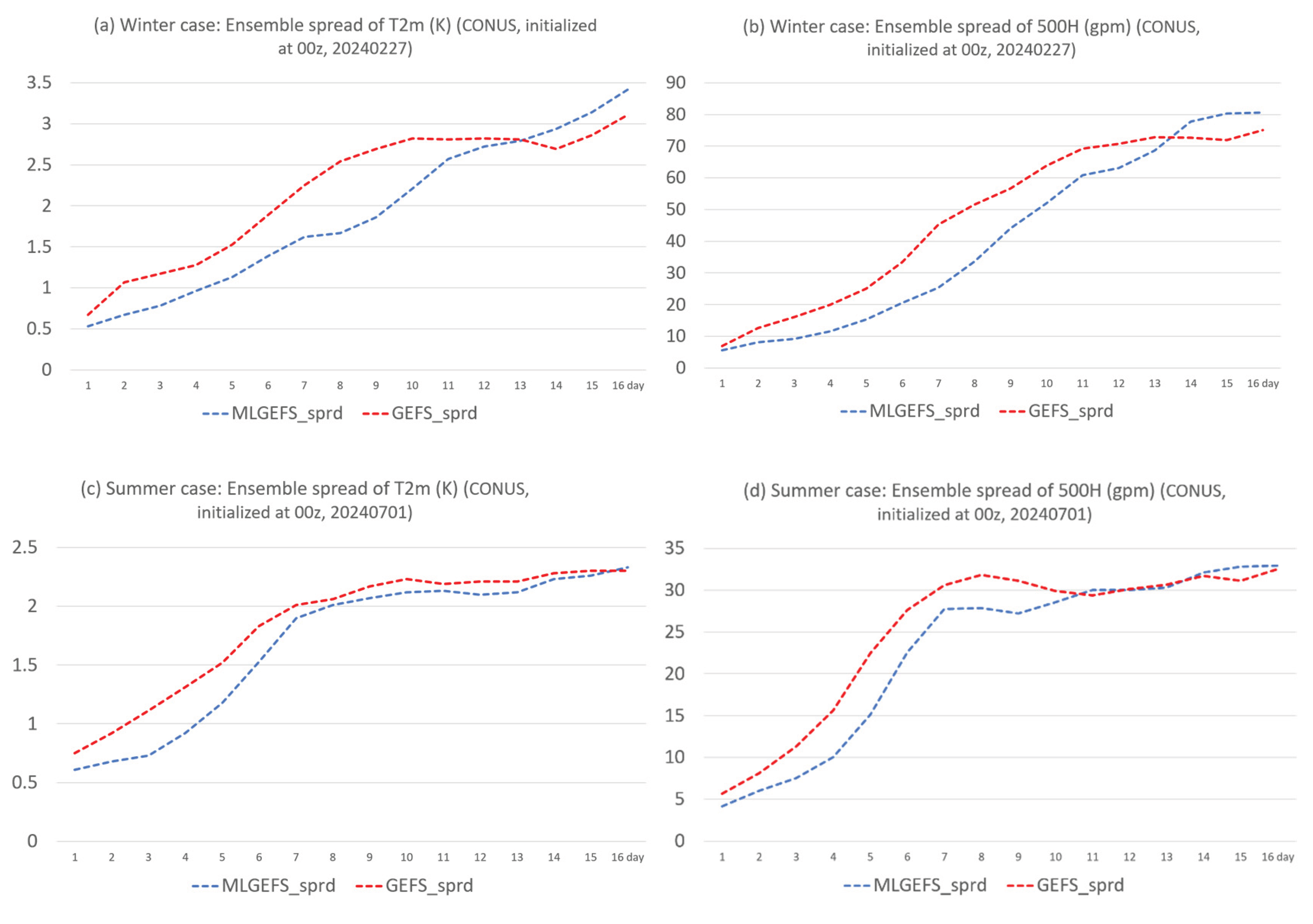
Figure 5.
(a) A winter example of ensemble spread (color shaded, unit: gpm) from MLGEFS’s 360hr forecast of 850H (initialized from 00z, Feb. 27, 2024). The black contour is the ensemble mean. (b) is the same as (a) but from GEFS. (c) A summer example of ensemble spread (color shaded, unit: gpm) from MLGEFS’s 384hr forecast of 850H (initialized from 00z, July 1, 2024). (d) is the same as (c) but from GEFS.
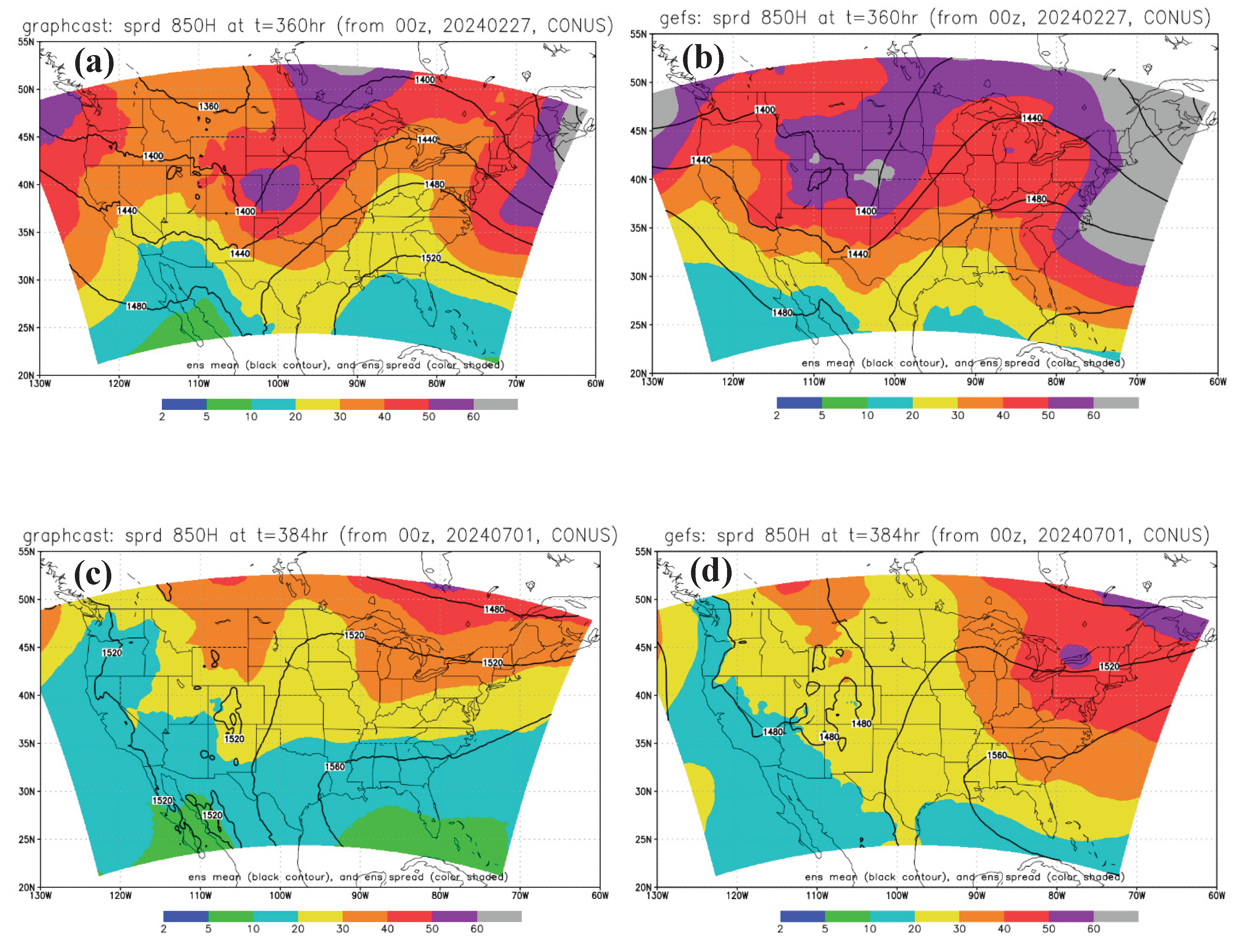
Figure 6.
Spatial correlation (y-axis) of ensemble spreads of 850H over the CONUS domain between MLGEFS and GEFS. Blue curve is for the winter case, and the red curve is for the summer case (red). X-axis is the forecast time (in days).
Figure 6.
Spatial correlation (y-axis) of ensemble spreads of 850H over the CONUS domain between MLGEFS and GEFS. Blue curve is for the winter case, and the red curve is for the summer case (red). X-axis is the forecast time (in days).
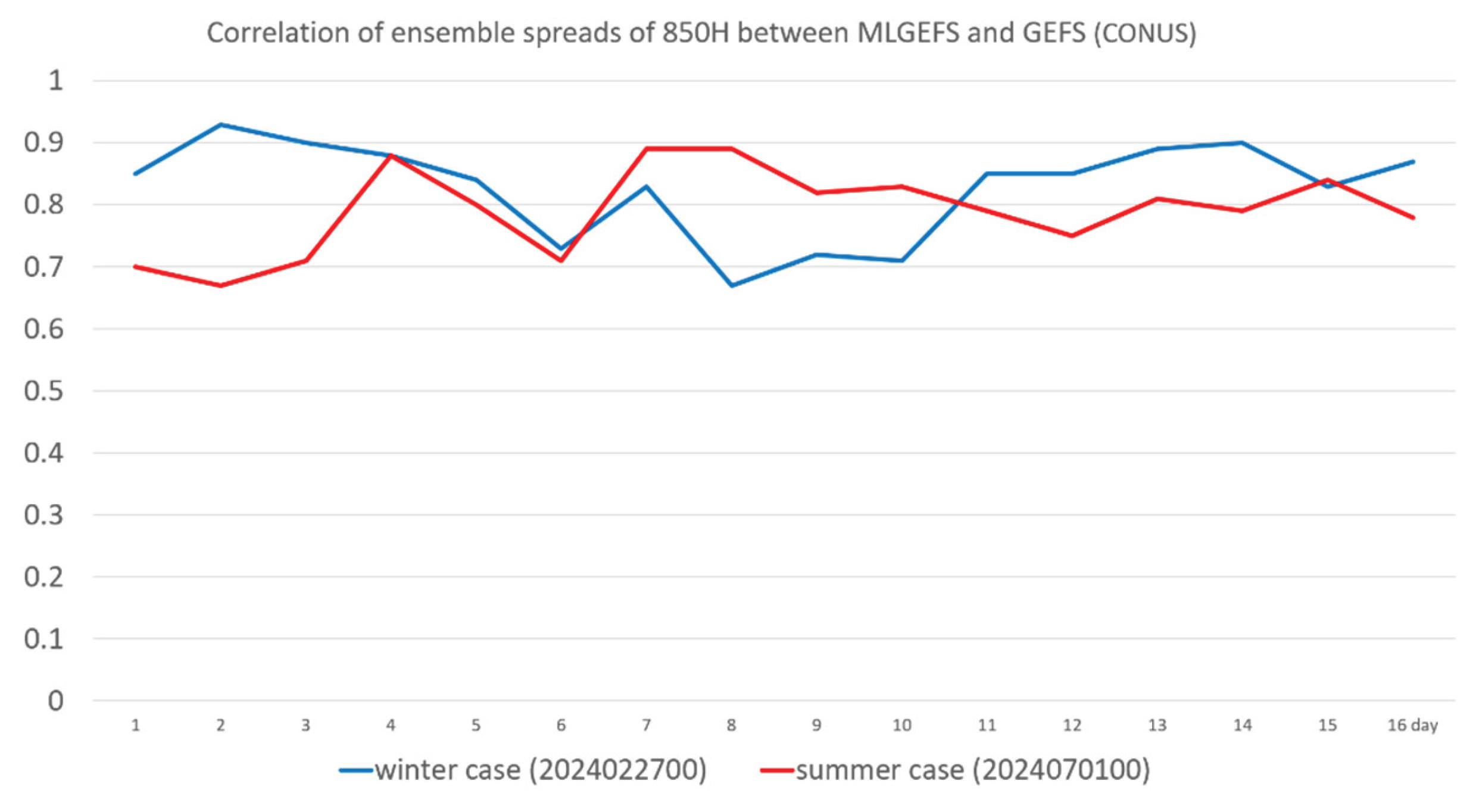
Figure 7.
Spatial correlation (y-axis) of ensemble spread with baroclinic instability (solid line) and convective instability (dash line) instability, respectively, over the CONUS domain for (a) T2m, and (b) 500H (red), in the winter case (initialized from 00z, Feb. 27, 2024). Blue lines are for MLGEFS and red lines for GEFS. (c) and (d) are the same as (a) and (b) but for the summer case (initialized from 00z, July 1, 2024). All forecast are projected into 16 days (384 hours). X-axis is the forecast time (in days).
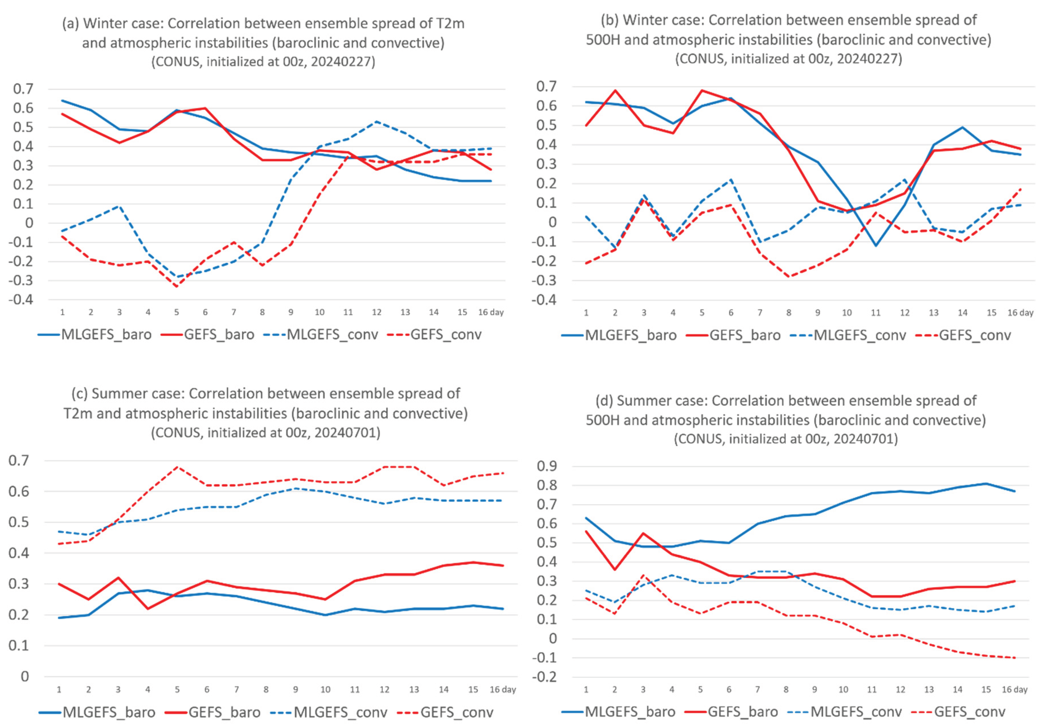
Figure 8.
Same as Figure 1 but for Consistency score (RMSE/spread). 1.0 is a perfect score.
Figure 8.
Same as Figure 1 but for Consistency score (RMSE/spread). 1.0 is a perfect score.
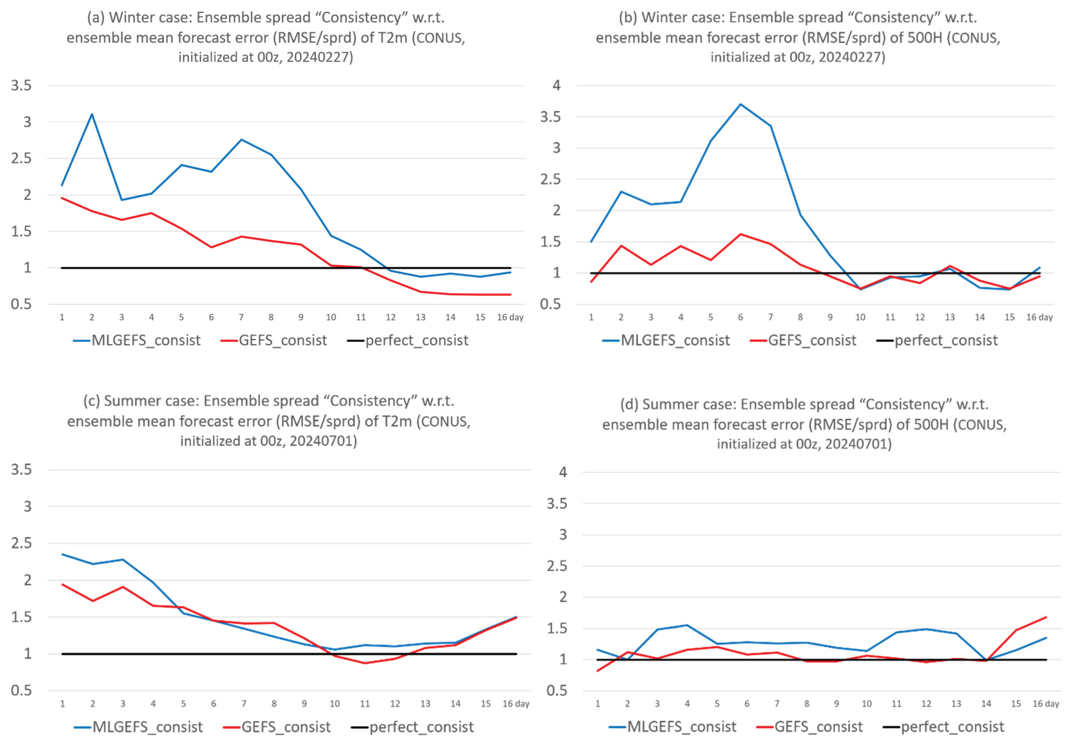
Figure 9.
Spatial correlation (y-axis) between ensemble spread and the absolute error of ensemble mean forecast over the CONUS domain for (a) T2m and (b) 500H from MLGEFS (blue curve) and GEFS (red curve), in the winter case (initialized from 00z, Feb. 27, 2024). (c) and (d) are the same as (a) and (b) but for the summer case (initialized from 00z, July 1, 2024). All forecasts are projected into 16 days (384 hours). X-axis is the forecast time (in days).
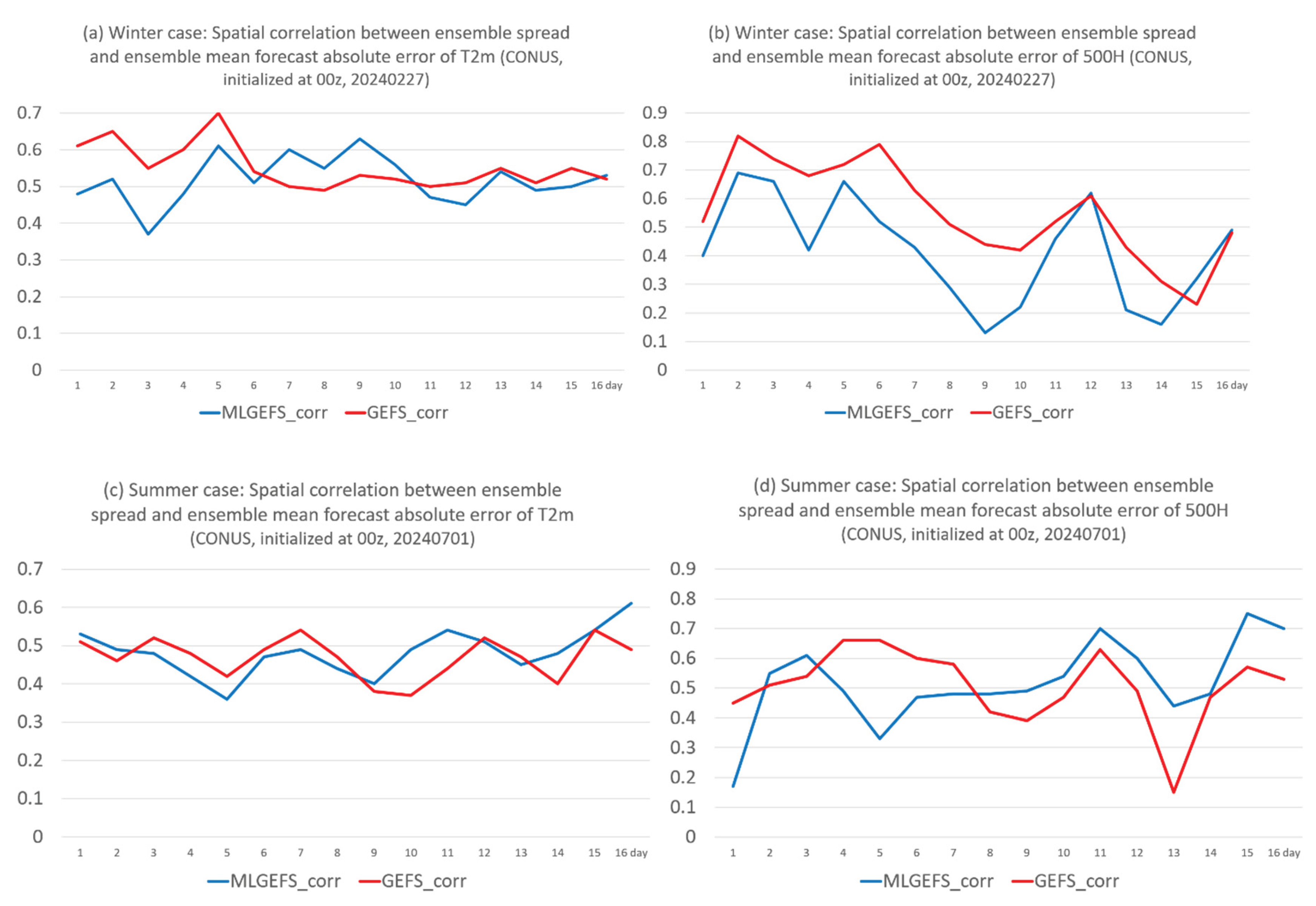
Figure 10.
Spatial correlation (y-axis) between different variables (T2m-SLP, and 500H-850T) in MLGEFS (solid line) and GEFS (dash line) over the CONUS domain for (a) the winter case (initialized from 00z, Feb. 27, 2024), and (b) the summer case (initialized from 00z, July 1, 2024). All forecast are projected into 16 days (384 hours). X-axis is the forecast time (in days).
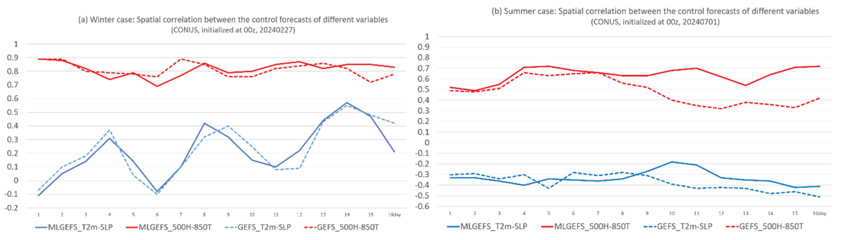
Figure 11.
Performance Rank Histogram (or Equal-likelihood histogram) of T2m, 500H, and SLP for (a) MLGEFS, and (b) GEFS forecasts over the 31 members (x-axis) at Day 7, in the winter case (initialized from 00z, Feb. 27, 2024). The values are averaged over the CONUS domain. Y-axis denotes the chance in %. (c) and (d) are the same as (a) and (b) but for the summer case (initialized from 00z, July 1, 2024).
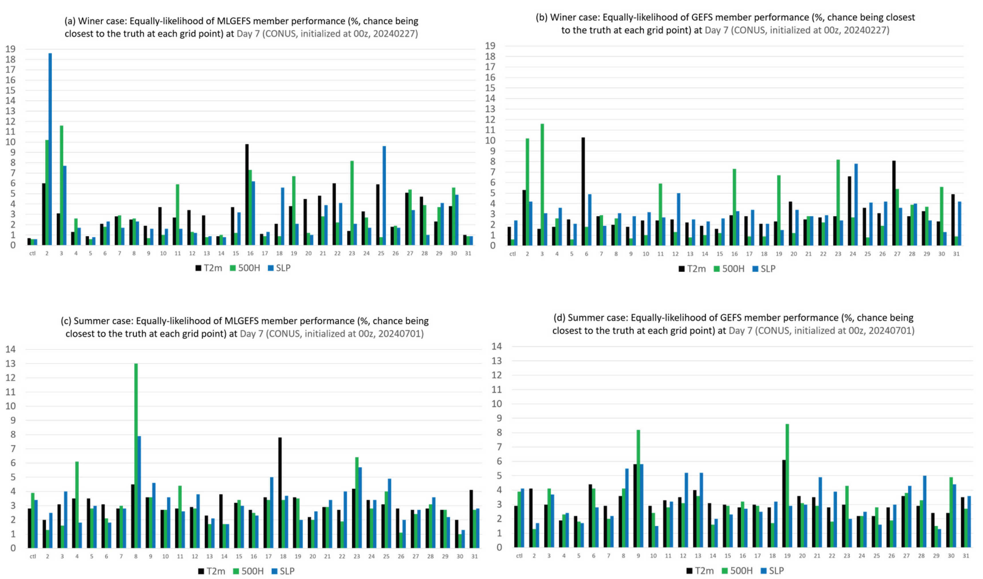
Figure 12.
Inter-variable correlation (y-axis) between their Performance Rank Histograms (such as Figure 11) of (a) T2m-500H, and (b) SLP-500H for MLGEFS (in blue) and GEFS (in red), from the winter case (initialized from 00z, Feb. 27, 2024). (c) and (d) are the same as (a) and (b) but for the summer case (initialized from 00z, July 1, 2024). All forecast are projected into 16 days (384 hours). X-axis is the forecast time (in days).
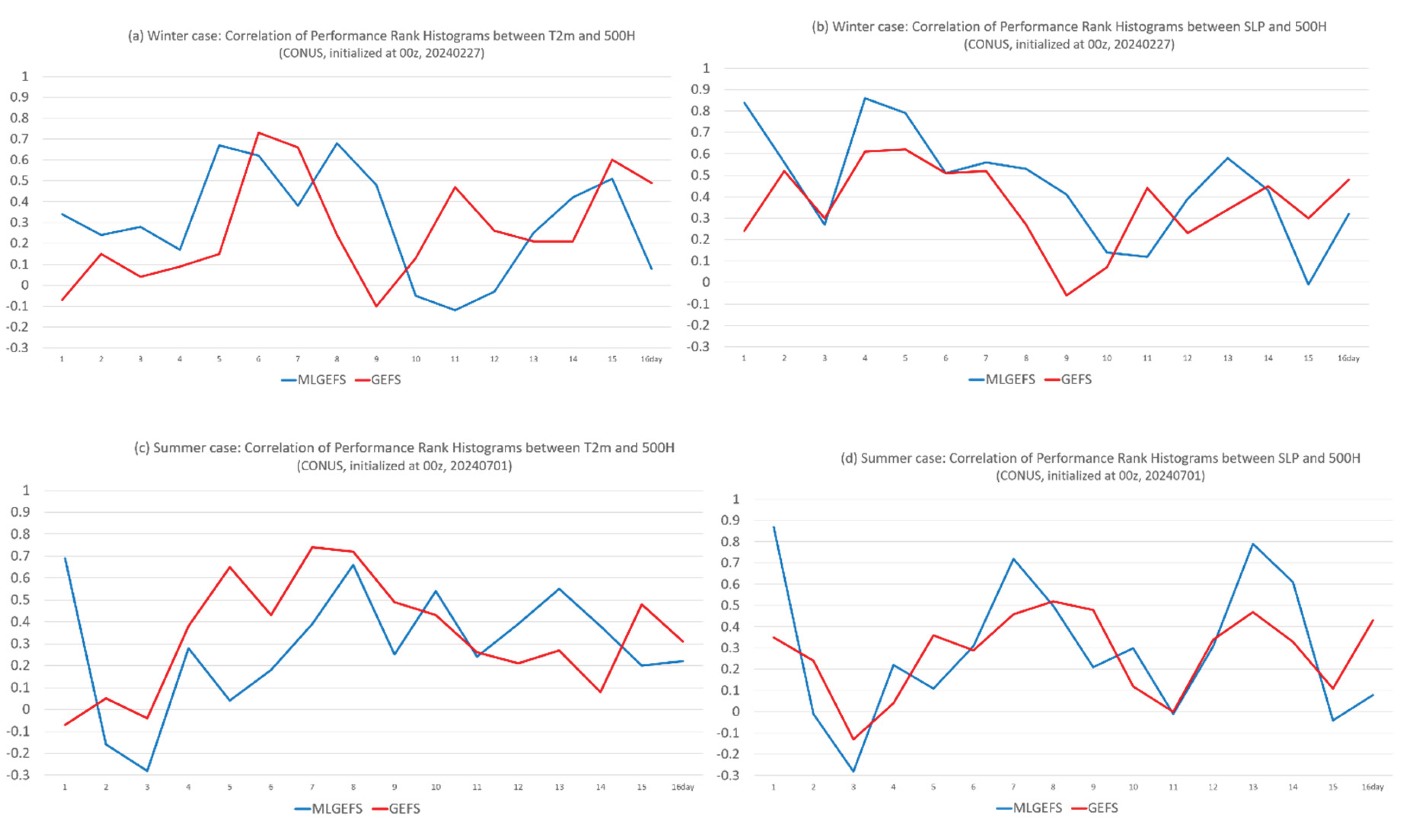
Figure 13.
Forecast error reduction (%, y-axis) of ensemble mean over control member of (a) T2m and (b) 500H for MLGEFS (in blue) and GEFS (in red), in the winter case (initialized from 00z, Feb. 27, 2024). The values are averaged over the CONUS domain. (c) and (d) are the same as (a) and (b) but for the summer case (initialized from 00z, July 1, 2024). All forecast are projected into 16 days (384 hours). X-axis is the forecast time (in days).
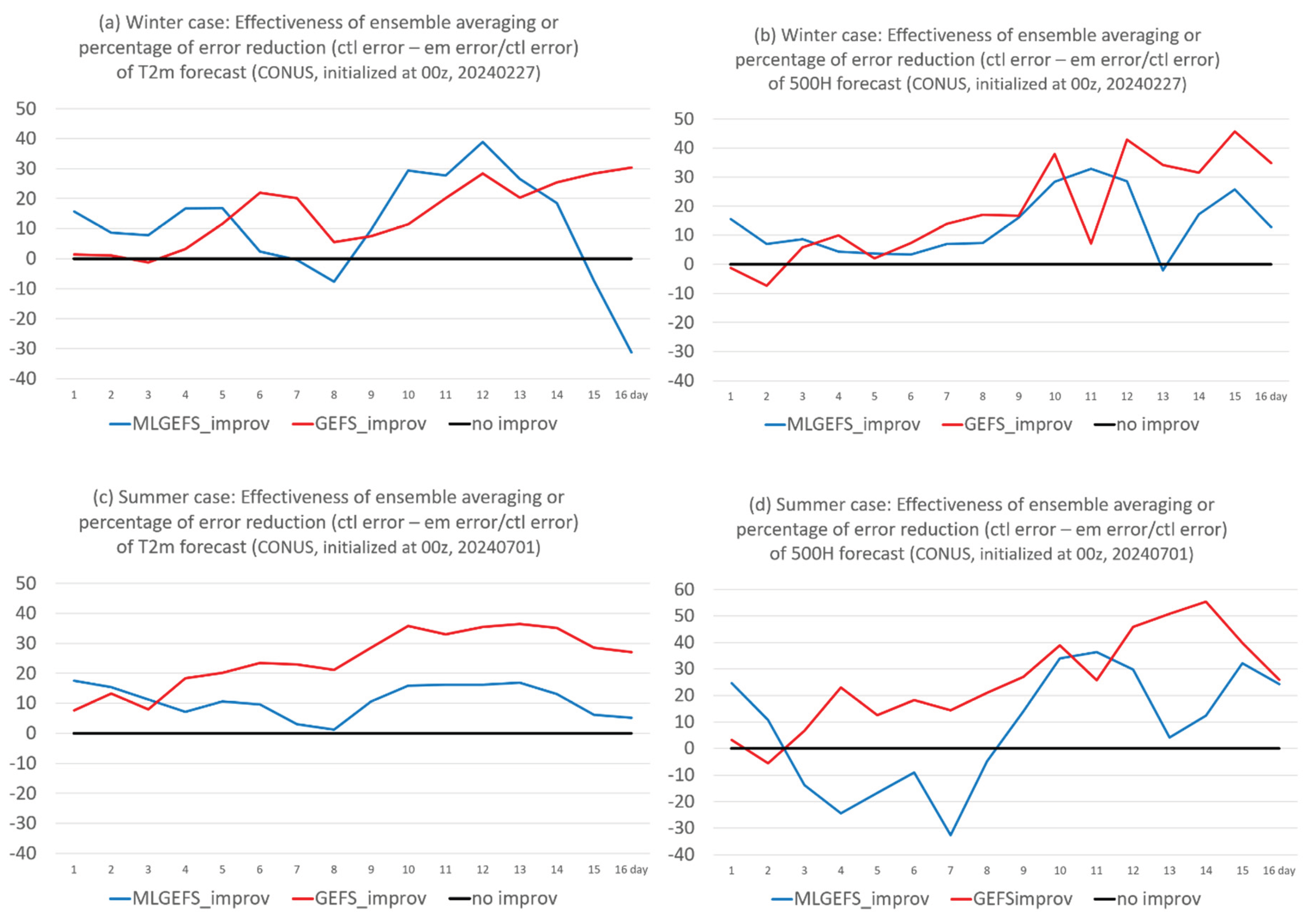
Figure 14.
Schematic diagram of ensemble members evolving with time, where control member is in blue, perturbed members are in black, and ensemble mean is in red. (a) Ensemble forecast 1 depicts the highly nonlinear situation, where members grow asymmetrically around the control member and the resulting ensemble mean is far away from the control. (b) Ensemble forecast 2 depicts the quasi-linear situation where members grow near symmetrically around the control member and the resulting ensemble mean is close to the control. .
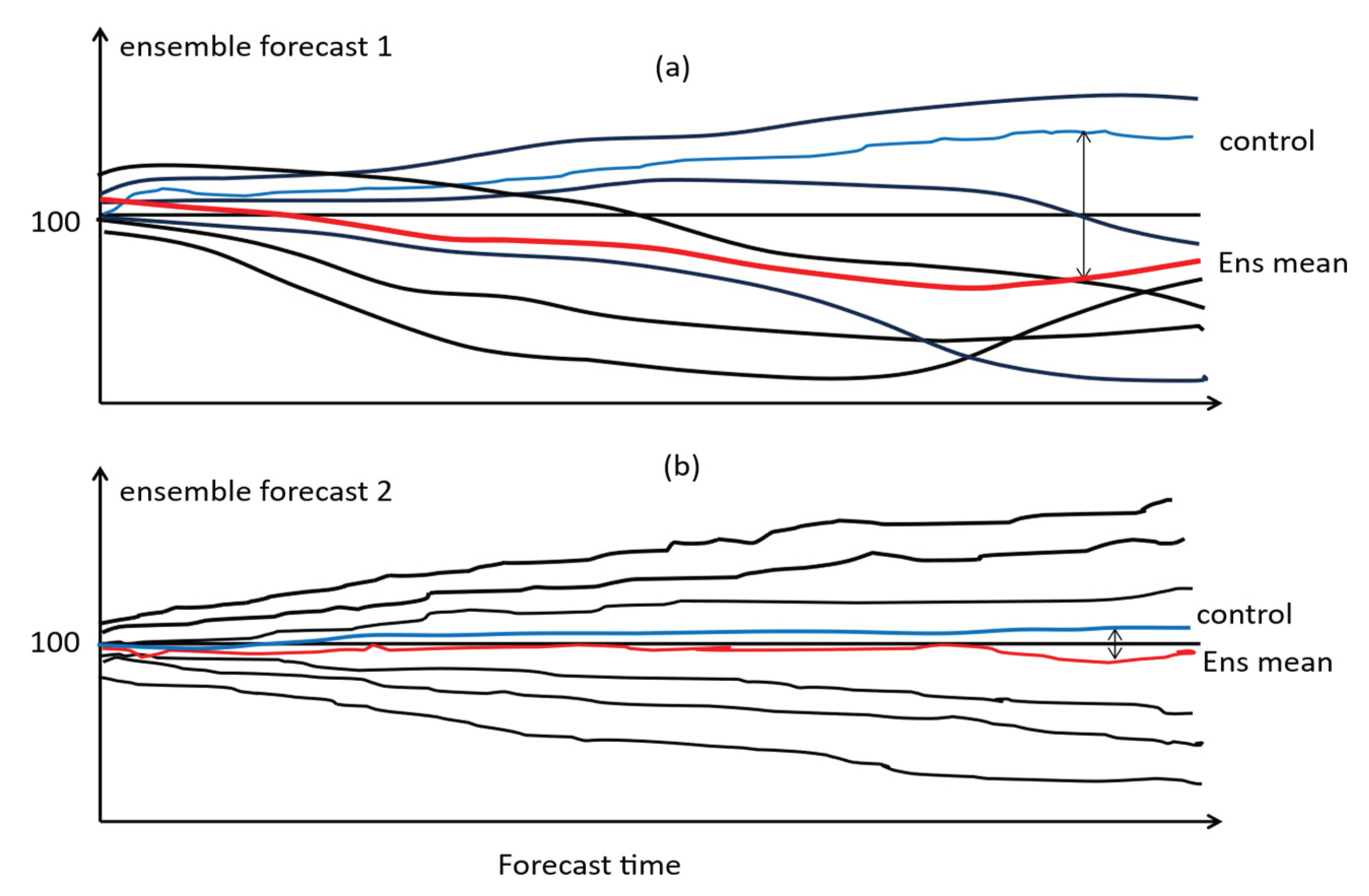
Figure 15.
Same as Figure 1 but for nonlinearity (Eq. 4).
Figure 15.
Same as Figure 1 but for nonlinearity (Eq. 4).
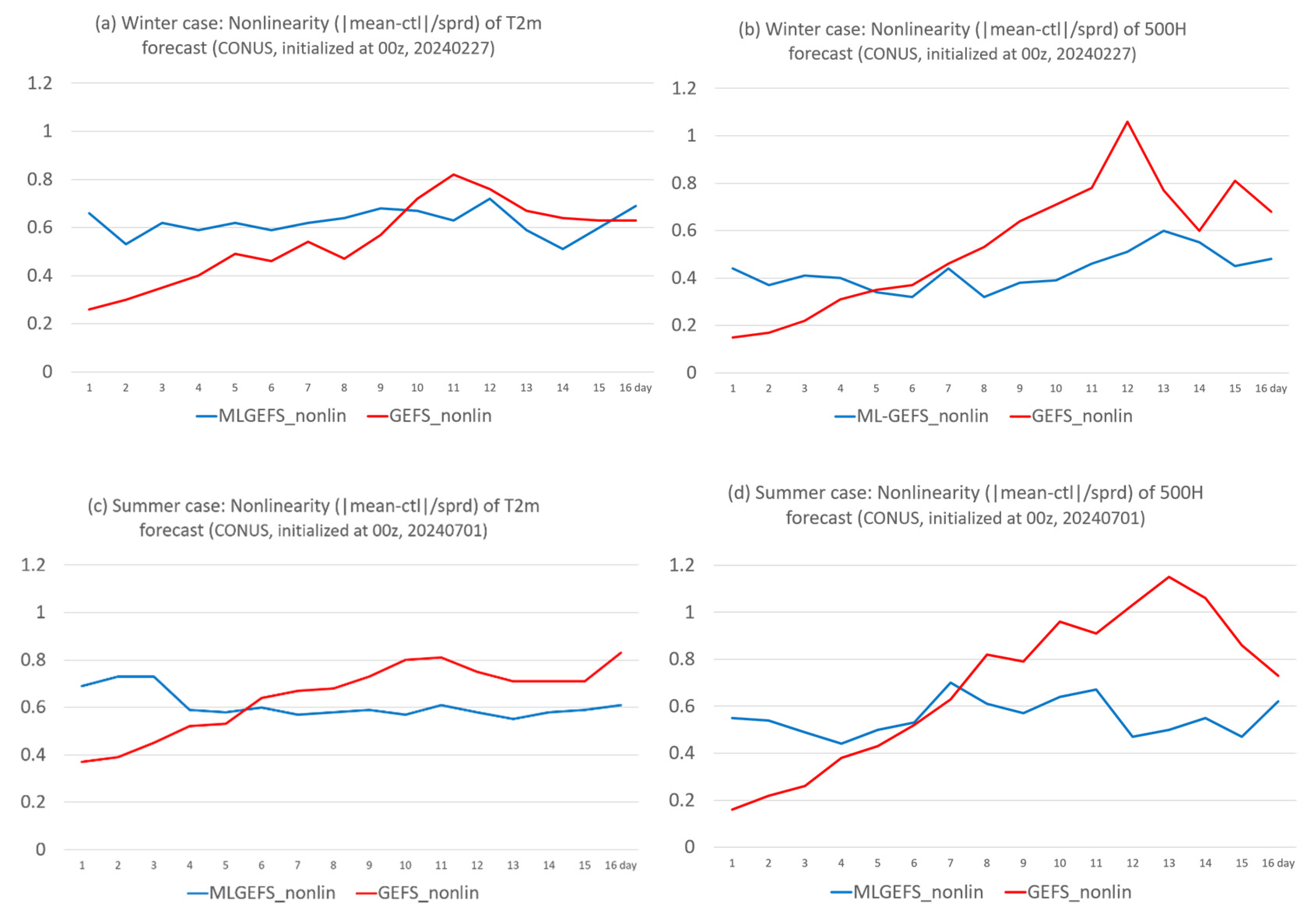
Figure 16.
Variation of PRVS (Performance Rank Variation Score, y-axis) with the separation distances (25, 50, 100, 200, 300, 400, and 500 km, x-axis) of (a) T2m and (b) 500H for the full member’s performance ranking at Day 1 (left panel), 10 (middle), and 16 (right), in the winter case (initialized from 00z, Feb. 27, 2024). The PRVS values are averaged over the CONUS domain. (c) and (d) are the same as (a) and (b) but for the summer case (initialized from 00z, July 1, 2024).
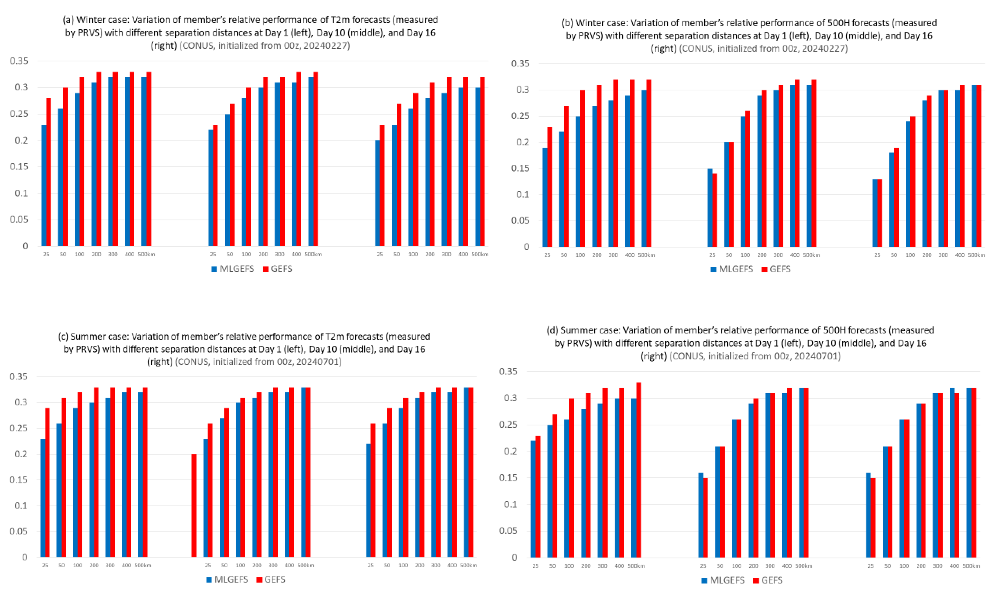
Figure 17.
An example of (a, b) 24h-accumulated precipitation forecast and (c, d) 500H from MLGEFS (left panel) and GEFS (right panel). They are 384h forecasts from the ensemble member #3 in the summer case (initialized from 00z, July 1, 2024).
Figure 17.
An example of (a, b) 24h-accumulated precipitation forecast and (c, d) 500H from MLGEFS (left panel) and GEFS (right panel). They are 384h forecasts from the ensemble member #3 in the summer case (initialized from 00z, July 1, 2024).
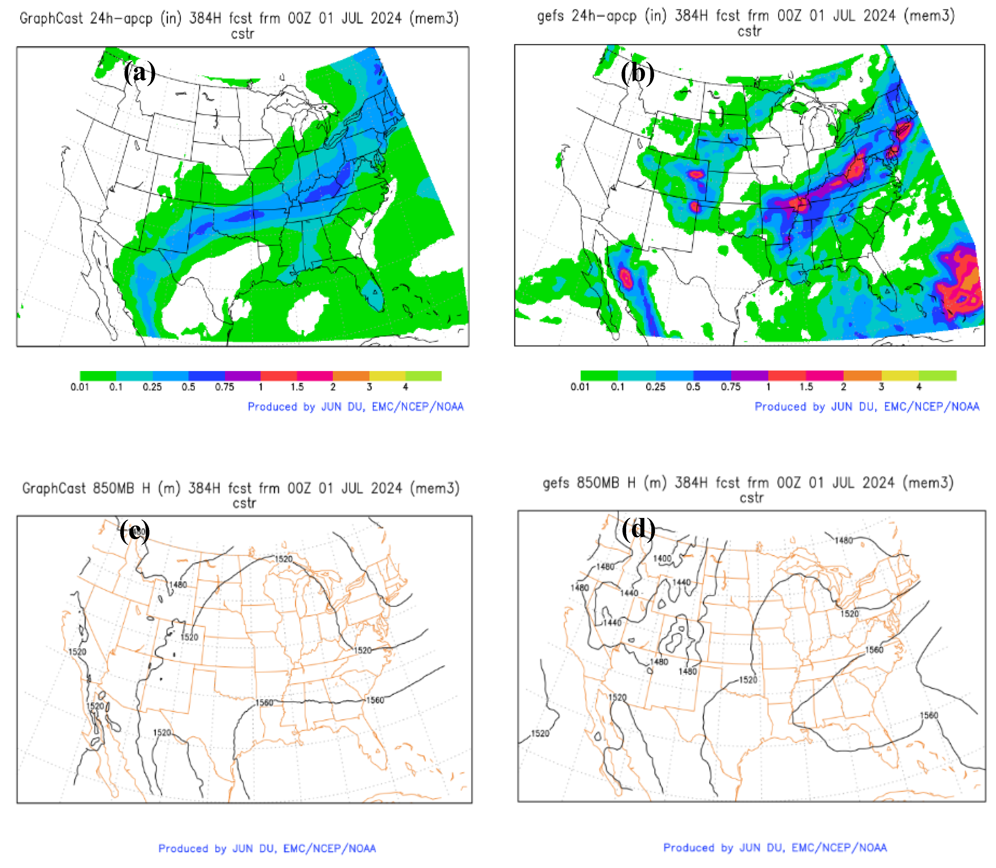
Figure 18.
Same as Figure 1 but for the spatial variation (Eq. 5).
Figure 18.
Same as Figure 1 but for the spatial variation (Eq. 5).
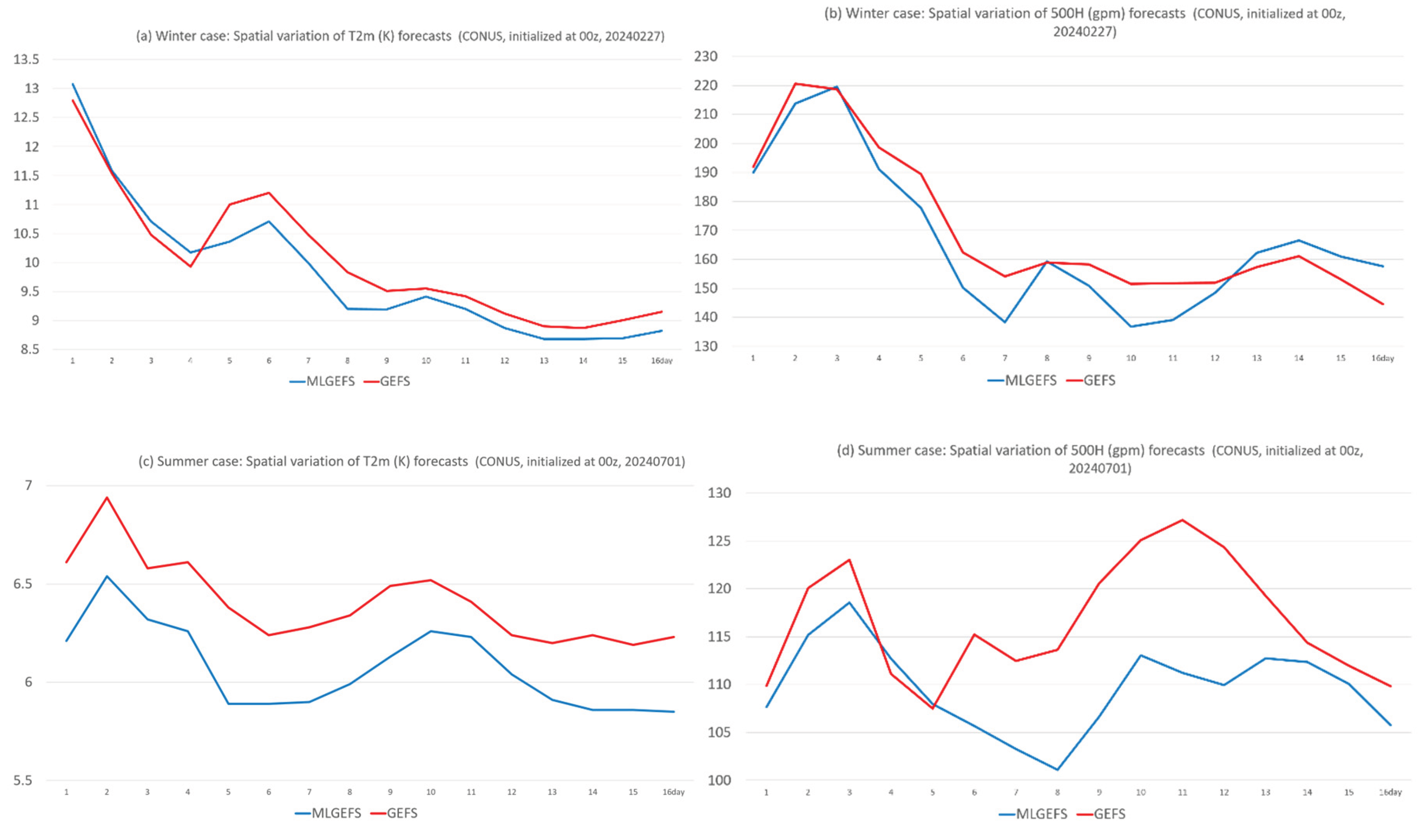
Figure 19.
Same as Figure 1 but for the absolute error of the statistical best member.
Figure 19.
Same as Figure 1 but for the absolute error of the statistical best member.
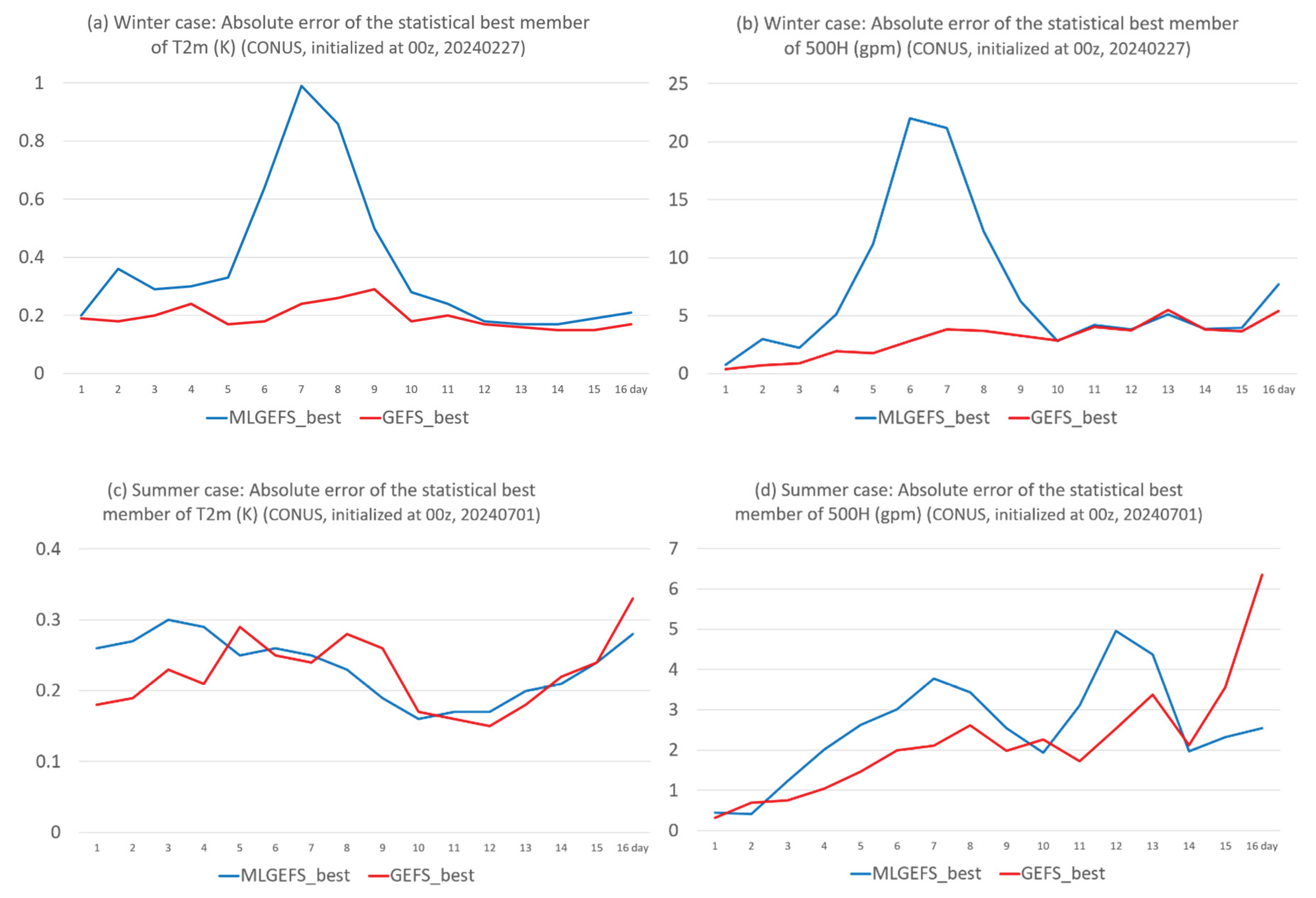
Figure 20.
Same as Figure 1 but for the absolute error of the statistical worst member.
Figure 20.
Same as Figure 1 but for the absolute error of the statistical worst member.
Disclaimer/Publisher’s Note: The statements, opinions and data contained in all publications are solely those of the individual author(s) and contributor(s) and not of MDPI and/or the editor(s). MDPI and/or the editor(s) disclaim responsibility for any injury to people or property resulting from any ideas, methods, instructions or products referred to in the content. |
© 2025 by the authors. Licensee MDPI, Basel, Switzerland. This article is an open access article distributed under the terms and conditions of the Creative Commons Attribution (CC BY) license (http://creativecommons.org/licenses/by/4.0/).
Copyright: This open access article is published under a Creative Commons CC BY 4.0 license, which permit the free download, distribution, and reuse, provided that the author and preprint are cited in any reuse.


