Submitted:
23 January 2026
Posted:
27 January 2026
You are already at the latest version
Abstract
In 1909, A. Einstein criticised Planck’s derivation of the radiation law, arguing that it relied on a seemingly absurd ('ungeheuerlich erscheinenden') assumption. The essence of his criticism lay in the observation that, within a blackbody, energy quanta corresponding to visible light are exceedingly rare even at comparatively high temperatures when measured against the number of molecules. Consequently, Planck’s entropy-based derivation appears unjustified, since at any given instant only an infinitesimal fraction of the possible energy distributions is actually realised. From this perspective, Planck’s approach should, in principle, lead to a result incompatible with experimental observation—yet it does not. In the present paper, Einstein’s criticism is analysed and quantified in detail. It is shown that the argument applies not only to Planck’s original derivation but also to alternative derivations of the radiation law, including Einstein’s own formulation of 1916. It therefore appears that Einstein’s riddle has not yet been solved. This is of particular relevance insofar as it may indicate that the distribution of energy among molecules is not governed by a stochastic process, but rather by an underlying deterministic mechanism. Such a conclusion would also have important implications for the interpretation of entropy. Further explanatory approaches are discussed. Finally, the role and relevance of intuitive models in physics are examined.
Keywords:
Planck
; Einstein
; radiation law
; photon
; light interference
; Copenhagen interpretation
; entropy
; energy distribution
; state distribution
Introduction
Quantum physics is founded, on the one hand, on the question of the stability of atoms. According to the laws of classical electrodynamics, an oscillating or orbiting (that is, accelerated) charge carrier—such as an electron moving in an orbit around an atomic core—should lose energy in the form of radiation. Electrons should therefore spiral into the atomic core (within a very short time), which is evidently not the case. On the other hand, quantum physics is based on the investigation of how matter interacts with electromagnetic radiation. A particular challenge in this context was the mathematical description of the continuous spectrum of black-body radiation, which M. Planck succeeded in providing in 1900 and 1901 [21,22], postulating the quantisation of energy. For his contemporaries, this marked the birth of quantum theory. Essential contributions to its further development were made initially by N. Bohr in 1913 with his idea of quantised electron orbits [5], and in particular by A. Einstein through the introduction of light quanta in 1905 [11], the application of energy quantisation to the specific heat of solids in 1907 [12], and the explanation of absorption and emission in 1916 and 1917 [14,15]. Further decisive input came from L. de Broglie in 1924 with the introduction of wave–particle duality [7].
In a second phase of its development, a mathematically consistent formulation of quantum theory was first achieved by W. Heisenberg in 1925 [20] with matrix mechanics (according to an alternative view, this had already been accomplished by G. Wentzel in 1924 [1,30] with his work on quantum optics). Another consistent formulation was presented by E. Schrödinger in 1926 [24]. This “modern quantum physics”, however, came at a price: it was accompanied by a reduction of physics to observable quantities and by a turning away from intuitive models. P. Dirac later expressed this position as follows [10]:
“Only questions about the results of experiments have a real significance and it is only such questions that theoretical physics has to consider.”
A central element of “modern quantum theory” is the possibility of considering superpositions of states, which are assumed to be real. Only through measurement is an event supposed to occur, the probability of which can be calculated by quantum theory. According to this interpretation, for example, an electron in a cloud chamber has a well-defined trajectory only because it is being continuously observed (or, more precisely, because it continuously undergoes observable interactions).
Not everyone agrees that science has taken the correct path here. It is, for example, as if all celestial phenomena could be described mathematically supported by a few additional rules (e. g., that there are in principle two types of wandering stars: I-planets and O-planets)—such as that some wandering stars remain in the vicinity of the Sun (the I-planets), that they suddenly change their direction of motion and form a loop (a large one in the case of the O-planets), that the light–dark axis of the Moon rotates over the course of the day, and so forth—without possessing, or even being allowed to seek, a heliocentric world view (or any other), and thus without an intuitive picture of the solar system. Can knowledge advance in this way? Can one extrapolate beyond the solar system, relying solely on mathematics and without an intuitive model—and, in the case of quantum mechanics, beyond the domain of established physics?
Some are sceptical in this regard. G. ’t Hooft, for example, has proposed in an interview a “new beginning right at the very start” [3]. A possible point of departure would be “classical quantum theory” (between 1900 and 1925), in which intuitive models still played a significant role. Particularly well suited as a starting point are the works of A. Einstein, who not only later criticised modern quantum theory (in 1935 together with Podolsky and N. Rosen, leading to the definition of entanglement [16]) but was also a critical participant in the early development of quantum theory itself. In this sense, a criticism from 1909 [13] concerning Planck’s derivation of the radiation law of 1900 [21] appears to the author to be especially relevant. I shall describe this criticism in more detail in the present paper and examine whether “Einstein’s riddle” has since been resolved. It may already be anticipated that this is unlikely to be the case—a circumstance that could be significant for the physical world view. Moreover, I aim to illustrate by example what consequences may arise from abandoning an intuitive model. Since a large part of the mathematics employed has already been developed in earlier works, I shall, for the convenience of the interested reader, take the unusual step of also indicating page numbers when citing certain publications.
Einstein’s Riddle
In 1909, A. Einstein confronted M. Planck [13] with the fact that his derivation of the radiation law, while leading to a result that is both mathematically correct and experimentally confirmed—namely (ρ: light intensity, mν: number of photons with frequency ν, h: Planck’s constant, c: speed of light, k: Boltzmann constant, T: temperature):
—nevertheless relies on an assumption that does not hold, that is, one which does not correspond to physical reality. Einstein’s objection is as follows (where W denotes the number of “complexions”, i.e. the different possible ways of distributing energy quanta ε among molecules or resonators):
“One could regard the number of complexions … as an expression for the multiplicity of possible distributions of the total energy among the N resonators only if every conceivable distribution of energy occurred, at least approximately, among the complexions used to calculate W. For this it is necessary that, for all ν to which a noticeable energy density ρ corresponds, the energy quantum ε be small compared with the mean resonator energy Ē. However, simple calculation shows that ε/Ē for the wavelength 0.5 μ and an absolute temperature T = 1700 is not only not small compared with 1, but even large compared with 1. … It is clear that … only a vanishingly small fraction of those energy distributions which we must regard as possible is taken into account in the calculation of the entropy. … In my opinion, accepting Planck’s theory means nothing less than abandoning the foundations of our theory of radiation.” (emphasis added and translated by the author)
According to M. Planck, ε = hν and Ē = hν / (exp(hν/kT) − 1). It follows that ε/Ē = exp(hν/kT) − 1. For the wavelength 0.5 μm and the absolute temperature T = 1700 K, A. Einstein obtained ε/Ē = 6.5 × 10⁷. Using the currently accepted values for h and k yields ε/Ē = 2.2 × 10⁷, a somewhat smaller number, which, however, does not invalidate Einstein’s argument. The reciprocal quantity, Ē/ε, corresponds to the number of energy quanta per molecule and is approximately Ē/ε = 4.5 × 10⁻⁸. This means that many of the possible permutations do not occur under the given conditions, and the calculation of entropy—which is a function of these complexions (S = k ln W)—must therefore lead to an incorrect result in a situation in which the number of quanta is exceedingly small in relation to the number of resonators. Remarkably, however, this is not the case.
Why M. Planck had to resort to entropy at all requires further explanation (Einstein’s criticism, incidentally, does not concern only the derivation of the radiation law itself, but also that of Planck’s formula ε = hν, and is therefore quite profound). The challenge faced by M. Planck is explained by A. Einstein in 1909 [13] as follows:
“Inside a cavity at temperature T there is radiation of a definite composition, independent of the nature of the body. Per unit volume of the cavity there is an amount of radiation ρ dν whose frequency lies between ν and ν + dν. The problem consists in determining ρ as a function of ν and T. If there is present in the cavity an electrical resonator of natural frequency ν₀ and weak damping, electromagnetic radiation theory allows the time average of the energy (Ē) to be determined as a function of temperature. This latter problem, however, can again be reduced to the following one. Suppose there are very many (N) resonators of frequency ν₀ present in the cavity. How does the entropy of this system of resonators depend on its energy?”
In the discussion of this contribution by Einstein, M. Planck emphasises:
“It is precisely emission and absorption [of light by matter] that constitute the obscure point about which we know very little”,
and accordingly, in his work of 1900 he did not attempt to model these processes (this was only done later by A. Einstein in 1916). In order nevertheless to arrive at a hypothesis concerning the interaction of electromagnetic radiation with matter, M. Planck was therefore compelled in 1900 [21] to employ a statistical model that had already been developed by L. Boltzmann in 1877 [4].
Boltzmann’s Model
In 1877, L. Boltzmann introduced, in a publication on the statistical interpretation of the second law of thermodynamics, a hypothesis that appeared very peculiar from the perspective of his time, namely the existence of discrete energy quanta ε [4].
“We assume that we have n molecules. Each of them shall be capable of possessing the kinetic energy 0, ε, 2ε, 3ε, …, pε, and these kinetic energies are to be distributed among the n molecules in all possible ways, subject to the condition that the total sum of the kinetic energy of all molecules always remains the same …”
Boltzmann (and later, in an analogous manner, M. Planck) then investigated the distribution of quanta of energy ε among molecules (or resonators) under the assumption that the random interactions by which molecules exchange quanta lead to a macroscopic equilibrium corresponding to the most probable energy distribution. However, which energy distribution is the most probable depends crucially on the nature of the interactions between the molecules.
As an example, in our macroscopic world we are accustomed to energy in the form of heat flowing from the body with higher energy to that with lower energy, that is, following the temperature gradient. If the same were true in the microscopic world—if quanta were therefore preferentially (more probably or more frequently) transferred from the molecule with higher energy to the one with lower energy—the most probable energy or state distribution would be the uniform distribution, in which all molecules contain the same number of quanta. This distribution can be realised in only one way, whereas Boltzmann identified as the most probable that energy distribution which can be realised in the largest number of different ways.
To illustrate this, Boltzmann gave an example in his 1877 publication. If one wishes to distribute seven quanta among seven molecules, there is only one possibility in the case of uniform distribution: each molecule carries one quantum, 1111111. If, by contrast, three molecules have zero quanta, two have one quantum, and one each has two and three quanta, there exist more different possible arrangements (complexions or permutations)—namely 420—than for any other energy distribution: 0001123, 0010123, 0100123, and so forth, provided one assigns individuality to the molecules. Why one should do so is not explained by Boltzmann (the success of the method appears to justify the procedure). For the calculation of entropy, however, this is decisive, since apart from an additive constant it depends solely on the number of complexions.
Boltzmann’s considerations were purely statistical; he did not formulate any hypothesis as to how quanta are transferred from one molecule to another. It can be shown, however [27], that the Boltzmann energy distribution emerges if one assumes that, upon contact of two molecules, a single quantum is exchanged purely at random, entirely independently of how many quanta the participating molecules contain, provided this number is greater than zero (in the latter case, the molecule can act only as an acceptor, not as a donor). Although this is not how the process actually occurs, this kinetic model leads to the same result as Boltzmann obtained through statistical or combinatorial considerations.
Let N be the number of molecules and Q the number of quanta of energy ε distributed among the molecules, and let i denote the number of quanta per idealised molecule. Furthermore, we define nᵢ = Nᵢ/N and q = Q/N and describe the kinetics of the quantum exchange process as follows, assuming that the probability that two molecules meet depends on their abundance, but not on the number of quanta they contain.
An (i)-particle (a molecule with i quanta) is created when an (i–1)-particle absorbs a quantum [ni-1(1–n0)] or when an (i+1)-particle loses a quantum [ni+1]. Conversely, an (i)-particle is lost when an (i)-particle absorbs a quantum [ni(1–n0)] or when an (i)-particle loses a quantum [ni]. This yields the kinetic equation (i = 0, …, Q):
Δni/Δt = ni+1 – ni + (ni-1 – ni) (1–n0)
In equilibrium, Δni/Δt = 0, and therefore
ni+1 = ni + (ni – ni-1) (1–n0)
After a short calculation, one obtains
- 2)
- ni+1/ni = 1-n0
and finally (the mathematics of this kinetic model was derived in an earlier work by the author and is presented there in detail [27, pp. 7–9]):
- 3)
- n0=1/(1+q)
and
- 4)
- ni+1/ni = q/(1+q)
From this it follows that
- 5)
- ni=[1/(1+q)][q/(1+q)]i
Boltzmann [4] proved this result in 1877 only for the energy distribution with the largest number of complexions, whereas no such restriction arises from the kinetic model. If both the number of molecules and the number of quanta are large, this makes little difference, and in any case an exponential energy distribution results.
For Boltzmann, the introduction of energy quanta was merely a mathematical device: one could imagine the energy portions to be arbitrarily small and the number of quanta, relative to the number of molecules, to be very large. It then follows that q is also very large (q >> 1). Since
6) q/(1+q) = 1/(1+1/q)
one may, under these circumstances, approximate
7) ni+1/ni = exp(-1/q),
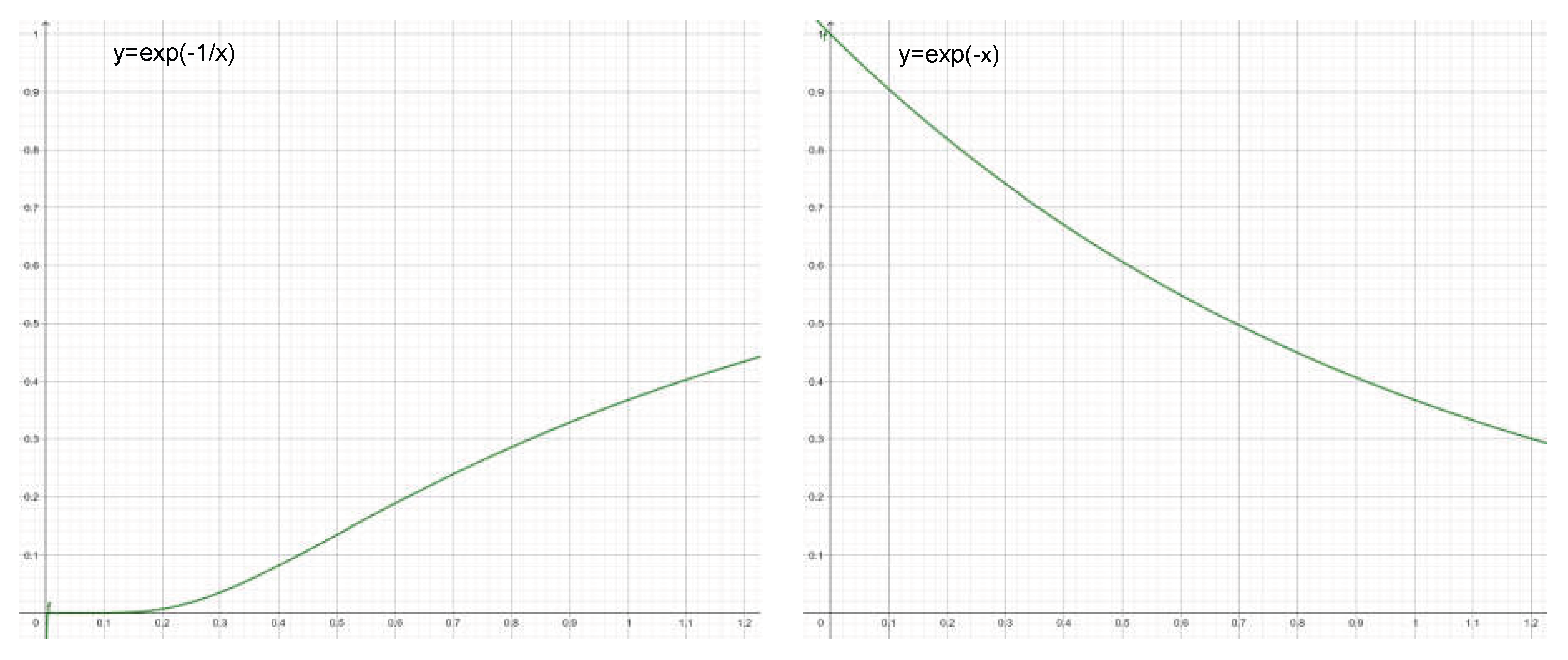
because the exponential function can be represented by a Taylor series, for whose first two terms one has exp(x)≈1+x. From this approximation the Boltzmann factor1 results by setting qε = kT (the temperature is proportional to the mean translational energy per molecule, while qε is the mean absorbed quantum energy; the hypothesis is thus formulated that, in the monochromatic model, the two are identical. Since in this model the energy quanta are purely a mathematical construct, there are no quanta of different energies). Equation (4) is the exact solution, whereas Eq. (7) is the approximation, which is correct only under certain conditions and predicts a more steeply decreasing energy distribution for small q (Figure 1).
Once it is recognised that energy quanta are real and not merely a mathematical device, one must ask whether the assumption q >> 1 is satisfied in nature. As A. Einstein calculated in 1909, this is definitely not the case for visible light; instead, q << 1 holds (quanta are indivisible, i.e. q = 0.3 means, for example, that on average three quanta are distributed over ten molecules). Accordingly, Eqs. (4) and (7) should yield very different results under these conditions—which they do—and Eq. (4) should provide the correct result, while Eq. (7) should give an incorrect one. Yet this is not what happens. The approximation describes nature and agrees with experimental findings, whereas the exact equation does not. This is what struck A. Einstein in 1909 and what I refer to here as Einstein’s riddle. The presentation chosen here differs from Einstein’s original one (in particular, entropy has not been used), but it is entirely equivalent to his argument and easier to quantify.
That Eq. (7) constitutes an acceptable approximation to Eq. (4) can also be shown by equating the two: q/(1+q)=exp(-1/q). This then yields for Euler’s number e=(1+1/q)q, which indeed holds for q → ∞.
In this way one can also investigate whether the energy distribution of two-state systems—systems that, with respect to a given quantum or energy level, can only be either in the ground state (Z₀) or in the excited state (Z₁), and can therefore absorb at most one quantum of a given “colour” or energy ε—can be approximated by the Boltzmann factor. In this case, n₁ = q and n₀ is the remainder, i.e. n₀ = 1 − q, from which, instead of Eq. (4), one obtains ni+1/ni=q/(1-q). Equating this with the exponential form yields q/(1-q)=exp(-1/q). For Euler’s number one then obtains e=(1/q-1)q, which is simply incorrect, regardless of the value assigned to q.
In general, atoms and molecules are described, with respect to a given colour or energy ε, as two-state systems, which is incompatible with the fact that their energy distribution can be approximately described by the Boltzmann factor. Nor does one obtain the radiation law for such systems, as will be shown later. This also affects considerations of an alternative definition of temperature (Atkins, 1986 [2]). We must therefore conclude: the interaction of light with matter, as well as the energy distribution in matter, presupposes resonators. This, too, is part of Einstein’s riddle.
Finally, A. Einstein concluded in 1909 [13]:
“Would it not be conceivable that, although the radiation formula given by Planck is correct, a derivation of it could be provided that does not rest on an assumption as seemingly absurd as that of Planck’s theory?”
He made an attempt in this direction in 1916 [14].
Einstein’s Model of the Interaction between Light and Matter (Blackbody)
In agreement with L. Boltzmann and M. Planck, A. Einstein described the (of course idealised) molecule in his model as a monochromatic resonator:
“Each molecule shall be capable only of a discrete sequence Z₁, Z₂, etc., of states with energy values ε₁, ε₂, etc.”
In addition to the ground state Z₀, there exist arbitrarily many excited states Zᵢ, with i ϵ ℕ₀⁺ (the states Zᵢ thus form a “ladder”). As we have already seen, this is the prerequisite for the distribution of energy among the molecules to be approximated by Eq. (7), and hence by the Boltzmann factor. Einstein further assumes thermal equilibrium.
In contrast to his predecessors, A. Einstein had very clear ideas about how molecules or resonators interact with one another (his model is kinetic rather than statistical). They do not interact directly at all; instead, they interact with a reservoir of free quanta—light quanta, later referred to as photons (the existence of light quanta was still denied by M. Planck in 1909 [13]). Photons can be absorbed or emitted by a molecule, involving a change in energy and momentum. From electromagnetic theory, Einstein inferred that there must be three elementary processes of this kind: absorption, as well as spontaneous and stimulated emission (Figure 2). He compared spontaneous emission to radioactive decay; it occurs without external influence. Since, within electromagnetic theory, a resonator can both absorb energy from the field and release energy into it, the same must also be possible in quantum theory. Consequently, a light quantum can be absorbed and can also trigger the emission of another photon of the same energy ε.
For the model we therefore require three kinetic constants: α for absorption, β for stimulated emission, and γ for spontaneous emission. In contrast to A. Einstein (1916) [14], I additionally introduce a fourth constant, δ, which describes the interaction probability between molecule and photon, that is, the probability that a molecule and a photon encounter one another [27].
Furthermore, in addition to ni we also require the relative frequency of photons m, where m=M/N and M denotes the number of photons in the same volume to which the number of molecules N refers.
By considering the frequencies of emission events, in which a photon is created, and absorption events, in which one is lost, one arrives at an equation describing the change in the photon frequency (we assume that the probability that a photon and a molecule encounter one another depends on their respective abundances; that the absorption frequency is proportional to the light intensity and the number of molecules is not only intuitively obvious but also experimentally confirmed):
- A photon is created when one of the resonators emits one: δβ m(1–n₀) + γ(1–n₀). This is the sum of the frequencies of stimulated and spontaneous emission. Molecules in the 0-state have no photon and therefore cannot emit one.
- A light quantum, by contrast, is lost when any resonator absorbs one, which occurs with probability δα m (since Σnᵢ = 1).
This yields:
- 8)
- Δm/Δt = (1–n₀)(δβ m + γ) – δα m
Since, macroscopically, nothing changes in equilibrium, we have Δm/Δt = 0, which gives:
- 9)
- m = γ(1–n₀) / [δα – δβ(1–n₀)]
Einstein recognised in 1916 [14] that, in order to obtain Planck’s radiation law from his kinetic model, he had to assume that the kinetic constants for absorption and stimulated emission are equal, α = β. One then obtains for the relative photon number:
- 10)
- m = γ(1–n₀) / (δα n₀)
At this point the results of Boltzmann (1877) [4] can be employed, and this is precisely what Einstein did in 1916 in an analogous (though not identical to the one presented here) manner. First, Eq. 2 implies that n₀ = 1 − n₁/n₀. From this it follows:
11)
and after a short calculation:
12) According to Eq. 7 (together with the accompanying discussion), one has the approximation n₁/n₀ = exp(−ε/kT), and therefore
13)
Of course, the original paper [14] does not contain the parameter δ. According to Planck, moreover, ε = hν [22]. Is this procedure justified? The model of A. Einstein (1916) and that of L. Boltzmann (1877) are so different that one should not assume a specific energy distribution for the former. This is also unnecessary, since the state distribution can be derived directly from Einstein’s model. This is shown in detail in Ref. 27, pp. 11–15; a highly condensed version shall therefore suffice here. Just as the change in the photon frequency can be calculated, so too can that of molecules with i quanta, by calculating the frequencies of emission and absorption events. One obtains:
14) Δnᵢ/Δt = δα m nᵢ₋₁ + nᵢ₊₁(δβ m + γ) – nᵢ(δα m + δβ m + γ)
Once again we set Δnᵢ/Δt = 0 and α = β. This yields:
15) nᵢ₊₁ = [δα m(2nᵢ – nᵢ₋₁) + nᵢ γ] / (δα m + γ)
From Eq. 10 and Eq. 15 one finally obtains for the model [27]:
16) nᵢ₊₁/nᵢ = 1 − n₀
and
17) nᵢ₊₁/nᵢ = r/(1 + r),
with r = q − m. The quantity r therefore represents the mean number of quanta (or, equivalently, the mean energy) contained in a molecule and thus replaces q in Boltzmann’s model. In this way, Einstein’s model essentially yields the same state distribution as that obtained earlier by Boltzmann, which is reassuring, since it forms the foundation of thermodynamics. From Eq. 11 and Eq. 17 it follows:
18)
For large r one can, as already discussed, approximate nᵢ₊₁/nᵢ ≈ exp(−1/r). From Eq. 11, on the other hand, one obtains approximately:
19)
For r >> 1, Eqs. 18 and 19 agree well (Figure 3). However, as we know from Einstein (1909) [13], this condition is not fulfilled, for example, for visible light, and we therefore face the same dilemma as in Planck’s model. Einstein’s model does not resolve Einstein’s riddle, since here too Planck’s radiation law is obtained only if one uses the Boltzmann factor, which, under the given conditions, is an inadmissible approximation.
Even for a two-state system, Eq. 10 remains valid. However, here n1 = 1-n0, and thus, instead of Eqs. 16 and 17, we have:
20) n₁/n₀ = (1 – n₀)/n₀ = r/(1 – r)
Substituting into Eq. 10 yields:
21)
This equation does not correctly describe the interaction of light with matter, and we already know that two-state systems are also incompatible with the Boltzmann factor. To derive the radiation law, it is necessary to assume that molecules act as resonators—at least in the monochromatic model. R. Feynman’s derivation, which assumes that molecules with respect to a single “type of quantum” (colour) possess only a ground state (Z0) and an excited state (Z1), and which uses the Boltzmann factor, is therefore incorrect [17].
The Interaction of Molecule and Photon
According to Eqs. 1 and 13 the following applies:
22) γ / (δα) = 8πν² / c³
The right-hand side of this equation corresponds to the relation between the radiation density of the field and the average resonator energy. S. Bose paid particular attention to this in 1924 [6] and derived it from photon theory. He begins by noting that a photon in the direction of propagation (he naturally assumes that a light quantum has such a direction) carries a momentum of magnitude hν / c. Its instantaneous state is characterized by the spatial coordinates x, y, z and the corresponding momenta px, py, pz. Together, these form the coordinates of a point in phase space, with the obvious relation: px² + py² + pz² = h²ν² / c². Thus, for frequency ν in a unit volume, the corresponding region in phase space is 4πh³ν² / c³, as obtained by integrating over the spatial and momentum coordinates. Bose then divides the phase volume into cells of size h³, with the number of cells given by 4πν² / c³ and the volume of each cell given by the reciprocal of this number. In the same way that Debye did in 1910 [8], he then distributes the photons into the cells just as Boltzmann distributed energy quanta among molecules. This leads to the Planck radiation law. While Debye at least assumed the existence of a small piece of carbon, Bose’s hypothesis works entirely without matter. Finally, he doubles the number of cells to account for polarization.
However, Bose’s model does not solve Einstein’s riddle, because in his model, the relation between free quanta (photons) and the number of cells is the same as the relation between bound quanta and molecules in Einstein’s model.
I have two objections to his model: Planck’s law refers specifically to blackbody radiation, i.e., to very specific conditions. Hydrogen gas, for instance, radiates differently. Planck’s law describes the interaction of light with matter; the distribution of quanta occurs in the molecules, not in the field. Since the molecules in a blackbody are not polarizers and therefore absorb light equally well regardless of polarization, it also does not explain the discrepancy between the number of cells in his hypothesis and the right-hand side of Eq. 22.
In 2025, I made the rather unsuccessful attempt to treat photons as classical particles and, on this premise, to ask how likely it is for a molecule to encounter a light quantum [27]. This, of course, depends on the molecule and photon densities, which is already accounted for in Eqs. 8 and 14. Moreover, the probability of particles meeting in a time interval increases with their size and speed. We further assume that the speed and size of molecules are negligible compared to those of photons (visible light). Then the interaction probability depends only on the speed of light c and the cross-sectional size of the light quanta perpendicular to the propagation direction (along the direction of propagation, they effectively have zero extent at the speed of light due to Lorentz contraction). We assume a circular cross-section with radius λ / 2 (light is a transverse wave). This gives:
23) δ = π λ² c / 4
and because λν = c, it follows that:
24) δ = π c³ / 4 ν²
and consequently:
25)
If we assume that γ / α = 2, there remains a discrepancy of 1 / π² (perhaps an indication that the surface or interactivity of the photon changes periodically) between Eqs. 22 and 25, which does not simply follow from the assumption that photons follow classical trajectories. Nevertheless, if we accept the hypothesis that a photon behaves like a classical projectile, it follows that the cross-sectional area of the photon perpendicular to the propagation direction is, at least on average over time, only slightly more than one-tenth of the originally postulated area. Ultimately, one obtains the radiation law given in Eq. 1.
Absorption and Emission
Apart from the introduction of an additional constant δ, Einstein’s model can also be extended in other respects. In 1916, he postulated stimulated emission because, within the framework of electromagnetic theory, a resonator can both absorb energy from and emit energy into the field. Which of these occurs depends on the phase difference between the field and the resonator oscillation. It is therefore reasonable to incorporate this aspect into his model [26]. To do so, we replace γ/α = 2 with
26) γ = α + β,
where, for coherent light of blackbody radiation, it is assumed that α = β, as Einstein had to assume in order to derive the radiation law from his model. If the light is not coherent, we instead allow the kinetic “constants” for absorption and stimulated emission to take different values, while equation 26 is always assumed to hold.
To incorporate the significance of the phase difference between field and resonator oscillation into quantum theory, it is necessary to accept assumptions about photon properties originally formulated by De Raedt et al., 2005 [9]. Accordingly, the absorbed photon is assumed to transfer not only its energy but also its phase information φ to the molecule:
“We consider the photon to be a particle having an internal clock with one hand that rotates with a frequency f = ω/2π. … As the photon travels from one position in space to another, the clock encodes its time of flight t modulo the period 1/f. We therefore view the photon as a messenger carrying as message the position of the clock’s hand.”
If no spontaneous emission occurs beforehand, upon collision with a second photon its message is compared with the stored one. Depending on the magnitude of the phase difference ξij = φi − φj (i, j = 1,…, g), stimulated emission occurs with probability pij, resulting in the release of a photon pair with (nearly) identical properties (frequency, phase, polarization, trajectory). It is the attributes of the “later” photon that are adopted. The indices i and j refer to g different paths the photons may take in an interference experiment (for the double-slit experiment, g = 2). In interference experiments, of course, there is no thermal equilibrium and spontaneous emission plays a minor role. Let
27)
and let the relative frequency of photons carrying phase information φi be mi (Σmi = 1). Stimulated emission would correspond, in an interference experiment, to a detection event. Then the detection probability (here represented according to the Born rule as the square of the modulus of the probability amplitude A) is given by:
28)
Here again, we must assume a resonator (with many excited states) [26], so that the event (stimulated emission or detection) and its complementary event (absorption) can cancel each other out. Under these circumstances, and assuming equation 26 holds, for coherent light γ = 2α, because pij = 1/2. This is illustrated in Figure 4.
From Eq. 28 it follows:
29)
Equation 29 can be rearranged to yield [26, pp. 8–9]:
30)
The mathematical agreement with quantum theory is thus established, and the Born rule proves to be superfluous. However, it has been assumed here that (always two) different photons interfere with one another and that the approach is of a statistical nature. P. Dirac, by contrast, stated in 1947 [10]:
“Each photon … interferes only with itself. Interference between two different photons never occurs.”
And further:
“Some time before the discovery of quantum mechanics people realised that the connexion between light waves and photons must be of a statistical character. What they did not clearly realise, however, was that the wave function gives information about the probability of one photon being in a particular place and not the probable number of photons in that place.”
One might think that it is straightforward to devise an experiment that clarifies who is correct. For example, in the double-slit experiment one could replace a coherent light source by two sources of identical frequency and constant phase difference, such that photons passing through one slit originate only from the first source and those passing through the other slit only from the second source. If interference then occurs, the logical conclusion would be that Dirac is falsified. In fact, interference does occur, but in this case the Copenhagen interpretation explains it by stating that the possibilities interfere, not the photons themselves, provided that it is in principle impossible to distinguish from which source a photon originates. As long as the mathematics is correct, the Copenhagen interpretation ensures that the fundamental assumptions of quantum theory are not falsifiable.
Nevertheless, it may still be possible to falsify one of the two contradictory models by considering the interaction of quanta of different colours within a molecule. I proposed and outlined such an experiment in 2025 [28].
Within the interpretation presented here, one can dispense with the superposition of possibilities; instead, complementary events can mutually cancel each other. This, too, may turn out to be non-classical. Moreover, one must ask how it is possible for a photon to carry information about its travel duration, given that, according to relativity theory, no time elapses for a particle moving at the speed of light. Must one therefore assume that each photon possesses its own spacetime?
Order in Field and Matter
There is another aspect that we wish to examine in more detail, and to achieve this we return to Eq. 12:
If we rearrange this equation, we obtain:
31)
and hence:
32)
The ratio n₁/n₀ therefore represents the ratio between the number of stimulated emission events and the total number of emission events. This is significant because stimulated emission (δα m) generates coherent photon pairs, as demonstrated by the laser, whereas spontaneous emission (γ) produces photons of random phase (as well as propagation direction and polarisation). If the ratio between these two types of emission changes, the coherence state of the electromagnetic field also changes, because the relative number of coherent photon pairs is altered. The ratio n₁/n₀, and thus the fraction of stimulated emission, increases the larger q, the total number of quanta relative to the number of molecules, is. With increasing q, r—the number of quanta in the molecules relative to the number of molecules—also increases, and r in turn increases with temperature T. Taken together, this means that for photons of a given energy level ε, the average coherence of the field increases with temperature, while the order in matter decreases (entropy increases). Field coherence and entropy are measures of different kinds of order, or non-randomness [25, pp. 17-20]. For this reason, one cannot simply claim for the overall system that order decreases with increasing temperature; the key to how these two forms of order can be converted into one another presumably lies in Eq. 32.
These considerations are also relevant when it comes to explaining, within the present model, why an interference experiment can function even with an “incoherent” light source (such as the Sun), since a certain degree of coherence is unavoidable in the Einstein model.
For a given T, coherence in the field increases with decreasing frequency υ. This may explain why thermal diffusion through a narrow slit is more efficient at very low frequencies than is usually the case [19,23,29]. Under such conditions, a threshold may possibly be exceeded spontaneously, leading to a laser-like state; however, to the best of my knowledge, no model has yet investigated this possibility.
If A. Einstein was correct in asserting that molecules do not interact directly but always via the exchange of quanta, it may be possible that a significant fraction of macroscopic order can ultimately be traced back to Eq. 32.
Figure 5.
As the comparison with Eq. 32 shows, at a given frequency the fraction of stimulated emissions increases with increasing temperature (left x=kT/hν), while at a given temperature it decreases with increasing frequency and therefore increases with increasing wavelength (right x=hν/kT). (The graphic was created using GeoGebra.).
Feynman’s Derivation of the Radiation Law
Photons are bosons and therefore tend to occupy the same state. This property forms the basis of Feynman’s derivation of the radiation law [18]:
“The probability that an atom will emit a photon into a particular final state is increased by the factor (n+1) if there are already n photons in that state.”
He describes his model as follows:
“Suppose we imagine a situation in which photons are contained in a box—you can imagine a box with mirrors for walls. Now say that in the box we have n photons, all of the same state—the same frequency, direction, and polarization—so they can’t be distinguished, and that also there is an atom in the box that can emit another photon into the same state. Then the probability that it will emit a photon is (n+1)|a|², and the probability that it will absorb a photon is n|a|², where |a|² is the probability it would emit if no photons were present.”
It must be noted critically that in cavity radiation (or black-body radiation) the photons are not all in the same state, and that Feynman’s considerations should therefore not be relevant to this case (later, he explicitly calculates the number of photons in distinguishable states). As in Einstein’s model, the Boltzmann factor is not required here either; from Feynman’s model one can directly infer what the equilibrium energy distribution would look like if many atoms were present in the box: eventually, (almost) all photons would reside in the field and (almost) none in the atoms. This does not correspond to reality. Nevertheless, Feynman employs the Boltzmann factor to describe the energy distribution in matter, additionally treating the atoms as two-state systems—for which we already know that their state distribution cannot in fact be described by it. He thus simply combines mathematical results from different areas of physics until the desired result emerges. Why is this procedure accepted? The reason is that, at the time of his derivation, the use of intuitive models was no longer common practice in certain areas of physics. This, too, can be traced back to the Copenhagen interpretation.
How processes “actually” proceed, what is “really” going on, is no longer considered a subject of physics. Quantum theory in its modern form appears unable to contribute to the solution of Einstein’s riddle (if anything, it does the opposite), since in all derivations known to the author the Boltzmann factor or entropy must be employed.
Conclusions
The author is not aware of any derivation of Planck’s radiation law that does not, in one way or another, make use of entropy, the Boltzmann factor, or Bose–Einstein statistics. It therefore appears that Einstein’s riddle has not yet been solved. Obvious proposed solutions do not fit into established physics. One possibility is that the energy distribution in matter is not the result of a stochastic process, but of a deterministic one. This would, of course, also have consequences for the interpretation of entropy. However, it is entirely unclear what such a deterministic process might be. Could it, for instance, involve the internal molecular energy distribution?
If, on the other hand, a random process does underlie the state distribution, Einstein’s riddle implies either that the energy quanta exchanged are much smaller than assumed—which cannot be reconciled with what we believe we know about absorption and emission—or that the resonators are much larger than postulated, i.e. that they do not correspond to individual molecules but to ensembles. One assumption made by the author was that a photon “somehow” interacts not only with a single molecule but with all those it “touches”, in such a way that together they form a resonator [28]. Simple considerations show, however, that in this case the energy in the resonators would have to follow a chi-squared distribution, which rules out this possibility as well—at least in the form discussed here.
Another aim of the author was to demonstrate that we require intuitive models. A remarkable example is Einstein’s model, which can be extended in such a way that it accurately describes phenomena of both thermodynamics and quantum physics, even though both theories extend beyond the model in terms of their range of applicability. The model-free combination of mathematical formulae in order to obtain a desired result is unlikely to be a promising path forward.
| 1 | The Boltzmann factor describes the relationship between particle energies and their relative abundances as a function of the temperature T (where k is the Boltzmann constant and E the energy of the molecule).
|
References
- Antoci, S.; Liebscher, D.-E. The third way to quantum mechanics is the forgotten first. arXiv 1997, arXiv:physics/9704028, 1–17. [Google Scholar] [CrossRef]
- Atkins, P. W. The Second Law; Scientific American Library, 1984. [Google Scholar]
- Billings, L. Quantum Physics Is Nonsense: Theoretical Physicist Gerard ’t Hooft Reflects on the Future. Scientific American 2025, 333(1), 104–108. [Google Scholar] [CrossRef]
- Boltzmann, S. Über die Beziehung zwischen dem zweiten Hauptsatze der mechanischen Wärmetheorie und der Wahrscheinlichkeitsrechung respektive den Sätzen über das Wärmegleichgewicht. Sitzungsber. Kais. Akad. Wiss. Wien Math. Naturwiss. Classe 1877, 76, 373–435. [Google Scholar]
- Bohr, N. On the Constitution of Atoms and Molecules. Philosophical Magazine Series 1913, 6(26 (151)), 1–25. [Google Scholar] [CrossRef]
- Bose, S. Plancks Gesetz und Lichtquantenhypothese. Z. Physik 1924, 26, 178–181. [Google Scholar]
- de Broglie, L. A Tentative Theory of Light Quanta, The London, Edinburgh, and Dublin. Philosophical Magazine and Journal of Science 1924, 47, 446–458. [Google Scholar] [CrossRef]
- Debye, P. Der Wahrscheinlichkeitsbegriff in der Theorie der Strahlung. Annalen der Physik 338(16), 1427–1434, 1910. [CrossRef]
- De Raedt, H.; De Raedt, K.; Michielsen, K. Event-based simulation of single-photon beam splitters and Mach-Zehnder interferometers. arXiv 2005, arXiv:quant. [Google Scholar] [CrossRef]
- Dirak, P. A. M. The Principles of Quantum Mechanics, Third Edition; Clarendon Press: Oxford, 1947. [Google Scholar]
- Einstein, A. Über einen die Erzeugung und Verwandlung des Lichtes betreffenden heuristischen Gesichtspunkt. Ann. Phys. 1905, 322(6), 132–148. [Google Scholar] [CrossRef]
- Einstein, A. Die Plancksche Theorie der Strahlung und die Theorie der spezifischen Wärme. Annalen der Physik 1907, 327(1), 180–190. [Google Scholar] [CrossRef]
- Einstein, A. Über die Entwicklung unserer Anschauung über das Wesen und die Konstitution der Strahlung. Physikalische Zeitschrift 1909, 22, 817–825. [Google Scholar]
- Einstein, A. Strahlungs-Emission und -Absortion nach der Quantentheorie. Deutsche Physikalische Gesellschaft, Verhandlungen 1916, 13/14, 318–323. [Google Scholar]
- Einstein, A. Zur Quantentheorie der Strahlung. Physikalische Zeitschrift 1917, 18, 121–128. [Google Scholar]
- Einstein, A. Can Quantum-Mechanical Description of Physical Reality Be Considered Complete? Physical Review 1935, 47, 777–780. [Google Scholar] [CrossRef]
- Feynman, R. P.; Leighton, R. B.; Sands, M. The Feynman Lectures on Physics, Volume I. Available online: https://www.feynmanlectures.caltech.edu/.
- Feynman, R. P.; Leighton, R. B.; Sands, M. The Feynman Lectures on Physics, Volume III. Available online: https://www.feynmanlectures.caltech.edu/.
- Geesmann, F.; Thurau, P.; Rodehutskors, S.; Ziehm, T.; Worbes, L.; Biehs, S.-A.; Kittel, A. Transition from Near-Field to Extreme Near-Field Radiative Heat Transfer. Physical Review Letters. [CrossRef] [PubMed]
- Heisenberg, W. Über quantentheoretische Umdeutung kinematischer und mechanischer Beziehungen. Zeitschrift für Physik 1925, 33, 879–893. [Google Scholar] [CrossRef]
- Planck, M. Zur Theorie des Gesetzes der Energieverteilung im Normalspektrum. Verhandlungen der Deutschen physikalischen Gesellschaft 2(17), 237–245, 1900.
- Planck, M. Über das Gesetz der Energieverteilung im Normalspektrum. Ann. Physik 4 553-563, 1901.
- Polder, D.; Van Hove, M. Theory of Radiative Heat Transfer between Closely Spaced Bodies. Phys. Rev. B 1971, 4, 3303–3314. [Google Scholar] [CrossRef]
- Schrödinger, E. Quantisierung als Eigenwertproblem. I-IV Annalen der Physik 79 79 80 81, 361-376 489-527 437-490 109-139, 1926.
- Tiefenbrunner, W. The Light Quantum as Replicator: Phase Copying by Photon-pair Interaction Mediated by Matter. MDPI-Preprints 2023, 1–23. [Google Scholar]
- Tiefenbrunner, W. The Interference of Light As Photon Pair Interaction Mediated by Matter Under the Assumption of Alternative (“Classical”) Photon Paths in Multi-path Experiments. MDPI-Preprints 2024, 2023020162. [Google Scholar] [CrossRef]
- Tiefenbrunner, W. The Monochromatic Resonator and the Interaction Between Light and Matter Under the Assumption That Photons Follow Classical Trajectories. MDPI-Preprints 2025, 2025021648. [Google Scholar] [CrossRef]
- Tiefenbrunner, W. The Shadow of a Laser Beam and the Interaction of Light with Matter. MDPI-Preprints 2025, 2025080965. [Google Scholar] [CrossRef]
- Volokitin, A. I.; Persson, B. N. J. Near-field radiative heat transfer and noncontact friction. Rev. Mod. Phys. 2007, 79, 1291–1329. [Google Scholar] [CrossRef]
- Wentzel, G. Zur Quantenoptik. Zeitschrift für Physik 1924, 193–199. [Google Scholar] [CrossRef]
Figure 1.
Equations (4) and (7) yield different results for the energy distribution when the mean number of quanta per molecule is small, that is, for the ratio of the abundances of molecules whose energy content differs by only one quantum. (The figure was generated using GeoGebra.).
Figure 1.
Equations (4) and (7) yield different results for the energy distribution when the mean number of quanta per molecule is small, that is, for the ratio of the abundances of molecules whose energy content differs by only one quantum. (The figure was generated using GeoGebra.).
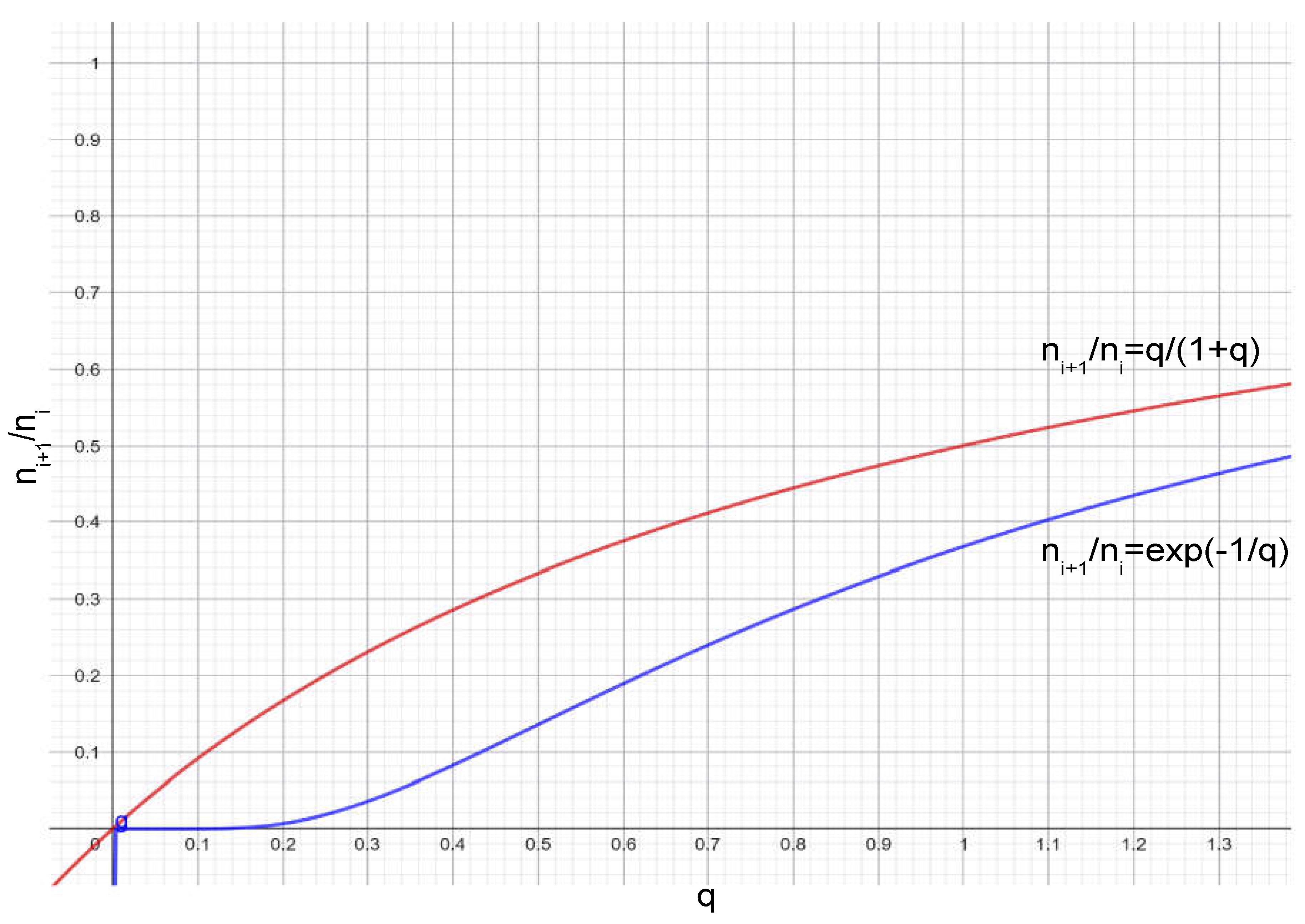
Figure 2.
Interaction of light and matter according to Einstein (1916) [14]. Two neighbouring energy levels (out of very many possible ones) of the molecule or monochromatic resonator are considered.
Figure 2.
Interaction of light and matter according to Einstein (1916) [14]. Two neighbouring energy levels (out of very many possible ones) of the molecule or monochromatic resonator are considered.
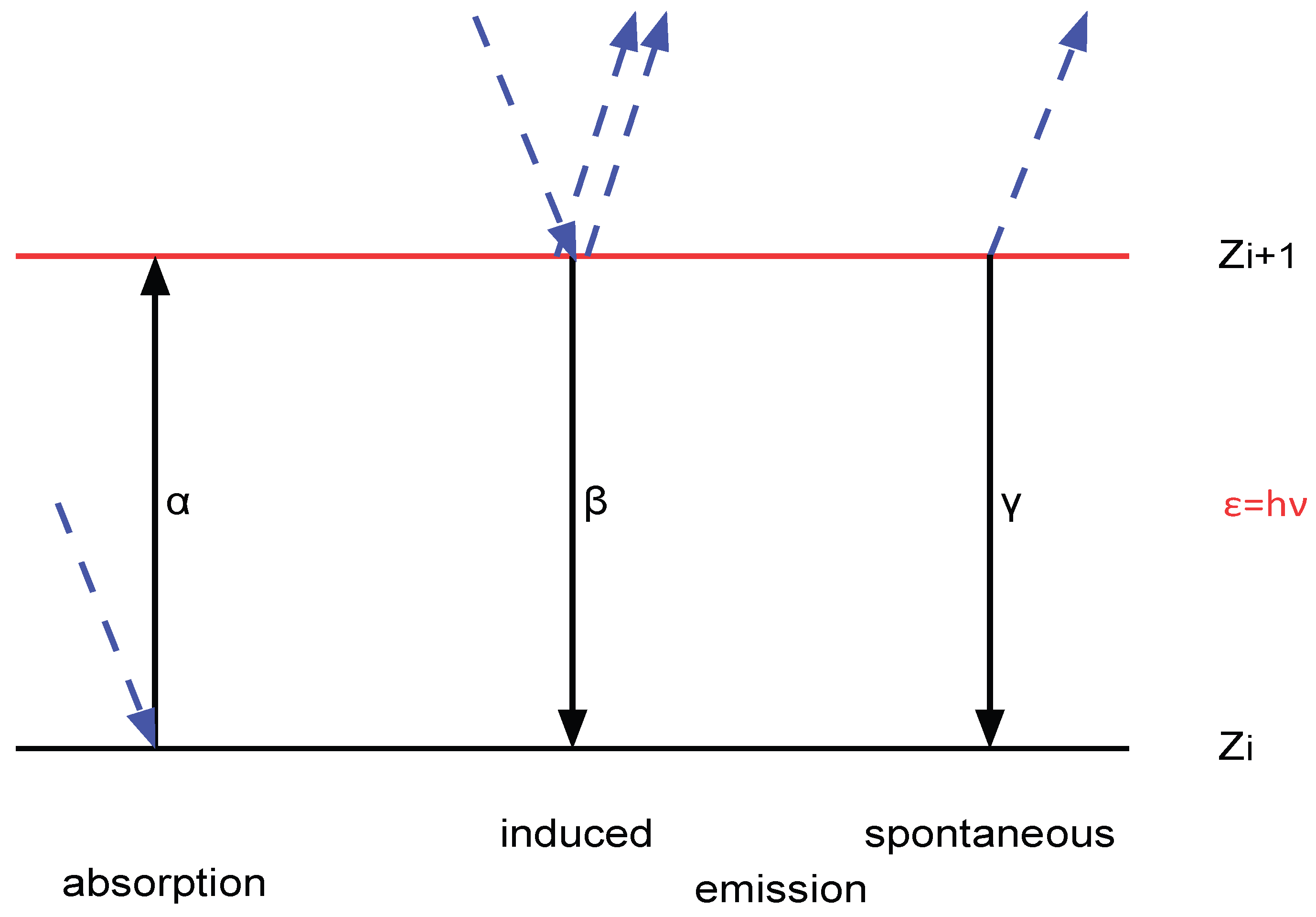
Figure 3.
Comparison of Eq. 18 with Eq. 19, i.e., of r with 1/(exp(1/r)-1), in the range between 0 and 100 on the one hand (left) and 0 and 1 on the other (right). (The graph was created using GeoGebra.).
Figure 3.
Comparison of Eq. 18 with Eq. 19, i.e., of r with 1/(exp(1/r)-1), in the range between 0 and 100 on the one hand (left) and 0 and 1 on the other (right). (The graph was created using GeoGebra.).
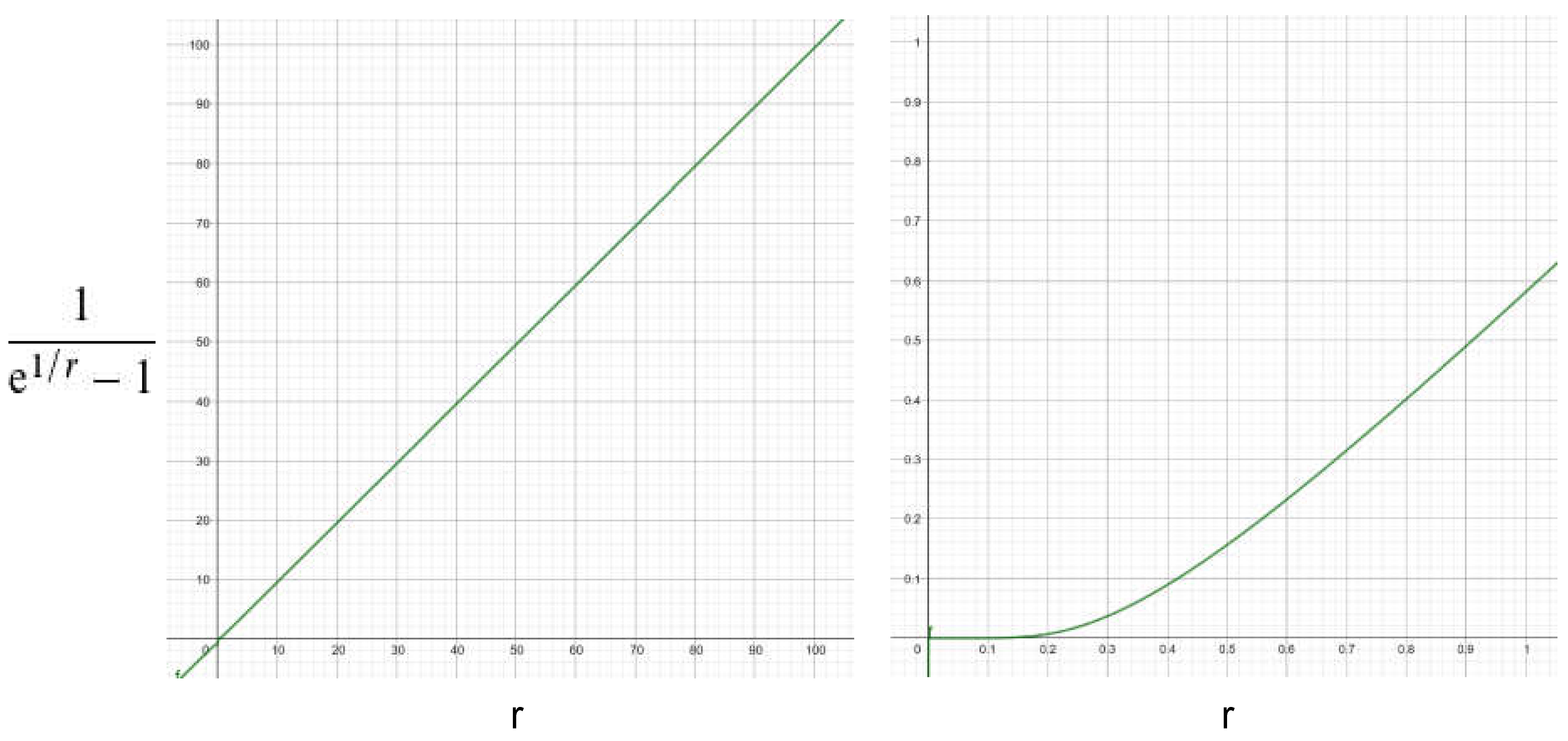
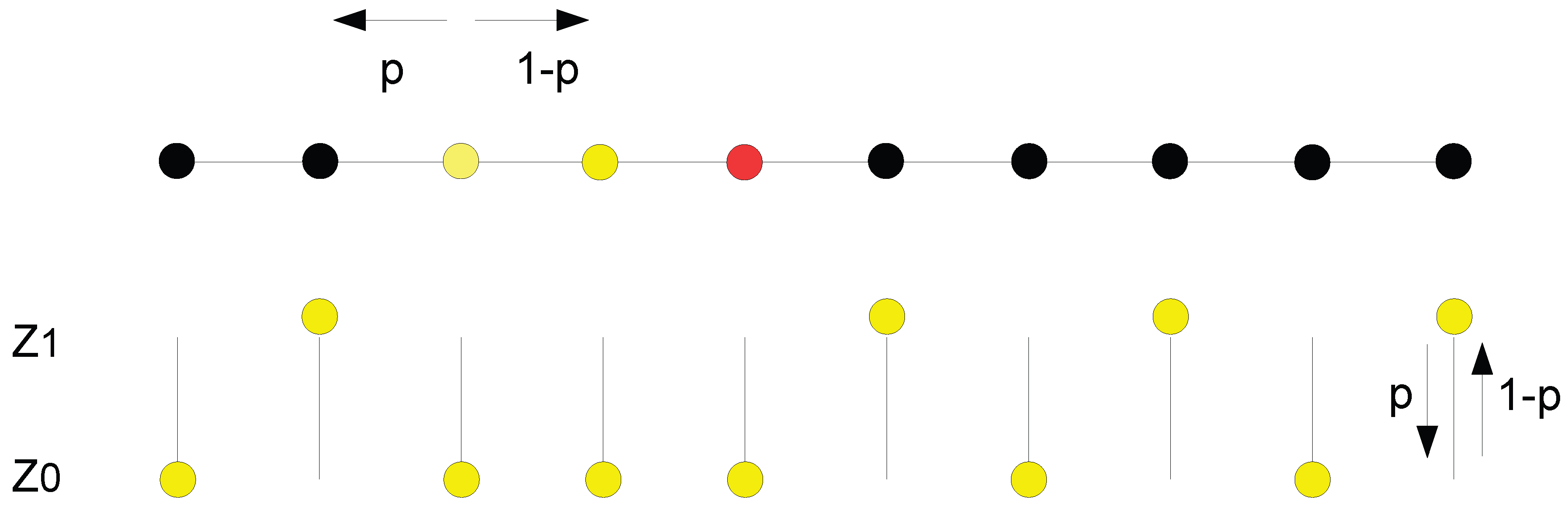
Figure 4.
In the resonator (top), absorption and stimulated emission events can mutually cancel each other (4–6 = −2, taking the red state as the initial state); the detection frequency follows from Eq. 29. For independent two-state systems this is not possible, because Z₀ can only absorb and Z₁ can only emit.
Disclaimer/Publisher’s Note: The statements, opinions and data contained in all publications are solely those of the individual author(s) and contributor(s) and not of MDPI and/or the editor(s). MDPI and/or the editor(s) disclaim responsibility for any injury to people or property resulting from any ideas, methods, instructions or products referred to in the content. |
© 2026 by the authors. Licensee MDPI, Basel, Switzerland. This article is an open access article distributed under the terms and conditions of the Creative Commons Attribution (CC BY) license (http://creativecommons.org/licenses/by/4.0/).
Copyright: This open access article is published under a Creative Commons CC BY 4.0 license, which permit the free download, distribution, and reuse, provided that the author and preprint are cited in any reuse.


