
Submitted:
23 January 2026
Posted:
26 January 2026
You are already at the latest version
Abstract
Optimal path tracking is a fundamental requirement for autonomous electric vehicles to ensure safety, stability, and driving comfort. This paper introduces a Prediction–Preview Cooperative Steering Control (MPC–PEM) method, which is a prediction-based steering control strategy designed to minimize lateral and heading errors. The approach utilizes a technique referred to as Preview Error Minimization (PEM). The controller predicts vehicle dynamics within a limited preview horizon to generate anticipative steering actions that adapt to road curvature and speed variations. A bicycle model is employed to represent the lateral–yaw dynamics, while the control law is formulated by considering system constraints and stability margins. Simulation results demonstrate that the proposed prediction–preview approach significantly improves tracking accuracy compared to conventional LQR and MPC methods, as evidenced by smaller heading and lateral errors, smoother steering angles, and more stable and realistic dynamic responses. This method offers an efficient, adaptive, and reliable steering control solution for the next generation of autonomous electric vehicles.
Keywords:
prediction-preview control
; steering control
; vehicle path tracking
; autonomous electric vehicles
; preview error minimization
; dynamic bicycle model
; lateral and yaw stability
; optimal control
1. Introduction
In recent years, the automotive industry has experienced a significant transformation fueled by the rapid advancement of technologies aimed at developing sustainable autonomous vehicle (AV) systems. AVs are projected to become the primary solution for future mass transportation systems due to their potential to enhance urban mobility efficiency by reducing traffic congestion [1] and increasing road capacity through intelligent inter-vehicle coordination [2]. Moreover, AVs contribute to driving comfort [3], energy sustainability [4], and improved road safety; both by reducing the risk of human-error-induced accidents [2] and by enhancing overall traffic safety [5,6]. Furthermore, AVs are recognized as a key component of the smart city ecosystem and Mobility-as-a-Service (MaaS) frameworks that rely on real-time data integration [7].
These technological advancements in AVs have stimulated intensive research, particularly in achieving highly accurate vehicle path tracking, especially when integrated with electric vehicles (EVs). Vehicle path tracking refers to a control algorithm designed to predict, follow, and guide a vehicle’s motion precisely under various operating conditions. The implementation of this method in AVs contributes to real-time maneuver stability, supports advanced driver-assistance systems (ADAS) to maintain lane discipline [8], and enables anticipation of future driving conditions [9]. In the context of autonomous electric vehicles (AEVs), the steering control system plays a pivotal role in ensuring the vehicle follows the desired path with minimal deviation, thereby guaranteeing stability, comfort, and navigation reliability.
In autonomous electric vehicles (AEVs), the connection between vehicle path tracking and steering control is critical since both systems operate dynamically and concurrently to ensure the vehicle follows the reference trajectory with high precision and accuracy. The vehicle path tracking subsystem uses sensor data to establish the vehicle's position, heading orientation, and optimum trajectory, whilst the steering control subsystem makes real-time steering angle adjustments to keep the vehicle in its lane. This interactive process enables the vehicle to compensate for trajectory deviations caused by rapid turns, quick maneuvers, or external influences such as lateral forces and variations in road friction coefficients [10,11,12]. Nevertheless, achieving highly accurate path tracking remains a major challenge, primarily due to the nonlinear of vehicle dynamics and constantly changing road conditions [13]. As a result, a more predictive and adaptive control strategy is necessary to provide constant tracking performance across numerous dynamic conditions.
Several control strategies have been developed to solve these issues. Classical approaches, such as the Proportional-Integral-Derivative (PID) and Linear Quadratic Regulator (LQR), are extensively employed due to their simplicity, but they have difficulties in dealing with dynamic fluctuations, which frequently result in overshoot and oscillations at high speeds [14,15,16]. More advanced techniques, such as Model Predictive Control (MPC) [17,18], fuzzy logic [19,20,21], sliding mode control (SMC) [22,23,24,25], and reinforcement learning (RL) [26], have shown promising gains in tracking accuracy. However, these solutions often need a lot of computational resources, rendering them unsuitable for use in embedded systems of electric vehicles [27].
Predictive techniques, such as preview control, are currently increasing popularity because to their capacity to foresee system dynamics and account for future reference trajectories, improving the vehicle's adaptive response to changing road conditions [28]. This method significantly reduces lateral and heading deviations, yielding steering signals that are more precise, smoother, and responsive to environmental changes [26]. One solution within this paradigm is Preview Error Minimization (PEM), which builds steering operations by projecting tracking mistakes over a short prediction horizon and proactively reducing them. This approach generates smooth and adaptive steering signals while being computationally efficient, making it ideal for real-time use in embedded systems [29].
Despite its high potential, significant research gaps exist. First, most conventional control approaches are still reactive and do not anticipate future system dynamics. Second, the use of preview-based path strategies in control design remains limited. Third, the implementation of the PEM algorithm in embedded devices with computing constraints has not been thoroughly investigated. As a result, there is an increasing demand for a control algorithm that is both precise and adaptable, as well as computationally economical, allowing for large-scale deployment inside modern autonomous vehicle (AV) architectures.
As a solution, this study proposes creating a predictive steering control system based on preview error minimization. The suggested controller generates more precise, smooth, and adaptive steering signals by combining future trajectory data, a vehicle lateral dynamics model, and a cost function to reduce lateral and orientation errors. This study's primary contributions include the following:
- Adapting a prediction-based steering control technique to reduce tracking error and yaw deviation by including Preview Error Minimization (PEM) for anticipatory directional control and smooth steering angle.
- Using a dynamic bicycle model to simulate lateral and yaw dynamics, taking into account system limits and stability margins.
- Validating the predictive-preview control method using detailed simulations that compare its performance to traditional LQR and MPC controls, exhibiting increases in tracking accuracy, steering signal smoothness, and vehicle stability.
- The prediction-preview approach to cooperative steering control strikes the ideal combination between predictive accuracy and dynamic stability, making it a viable solution for adaptive steering systems in modern autonomous cars.
This paper is organized as follows: Section 2 of this study describes the vehicle's lateral motion, which has been dynamically and kinematically modeled. Section 3 introduces prediction-preview-based steering control, which calculates the desired front wheel steering angle in real time while allowing for lateral and directional faults. Section 4 discusses vehicle path tracking, which includes environmental awareness, route planning, and tracking control. Section 5 presents the results and comments. The paper ends with a conclusion.
2. Vehicle Lateral Model
The performance of a vehicle path tracking technique is strongly dependent on the mathematical description of the vehicle's lateral dynamics, which a vehicle lateral model commonly represents. This model illustrates how steering angle, lateral tire force, slip angle, and yaw rate respond to steering actions. Integrating vehicle path tracking with lateral models enables the development of control rules that reduce position and heading orientation deviation while still maintaining lateral and yaw stability under a variety of dynamic circumstances. The accuracy and complexity of the lateral model have a direct impact on tracking performance, with kinematic models appropriate for low speeds and dynamic models better suited to high speeds and complex road conditions. Thus, the vehicle lateral model serves as an important predictive framework for vehicle path tracking, allowing it to create optimal, stable, and adaptive steering signals for the dynamics of autonomous electric vehicles.
Vehicle lateral models are commonly expressed in two ways: dynamic and kinematic. The lateral dynamic model is constructed by analyzing the forces operating on the vehicle and estimating the lateral acceleration and yaw rate reactions to steering inputs. Meanwhile, the lateral kinematic model is built based on the vehicle system's geometric relationships, and it is utilized to calculate the lateral error as well as the divergence of the vehicle's direction from the trajectory caused by steering wheel modifications.
The lateral model of this vehicle is frequently represented using a single-track model, sometimes known as a bicycle model, as illustrated in Figure 1. This model is made up of two coordinate systems: (i) a global coordinate system with XY axes that represents the vehicle's geometric movement in relation to the track and (ii) a vehicle coordinate system with xy axes that represents the vehicle's relative movement. In this model, point A represents the left and right rear wheel pairs united into a single virtual wheel, while point B represents the front wheel pair. Point O is specified as the vehicle's center of rotation, R is the radius of the vehicle's track, and cg is the vehicle's center of gravity. In addition, L symbolizes the wheelbase , which is made up of , the distance from the center of gravity to point B, and , the distance from the center of gravity to point A [10].
2.1. Lateral Vehicle Dynamic Model
Lateral vehicle dynamics include lateral and yaw motions. Figure 1 shows that lateral motion is caused by changes in the vehicle's translational force from the lateral axis (point O) to the center of gravity (cg), resulting in variations in the body side slip angle (). Yaw motion occurs as a vehicle turns, causing stiffness forces to change the yaw angle (), the body side slip angle (), and the front wheel steering angle (). Given a constant longitudinal vehicle velocity (), lateral vehicle dynamics are represented by a bicycle model with two degrees of freedom (2-DoF) based on lateral position () and yaw angle ().
The lateral position () is the distance along the lateral vehicle axis from point O, and the yaw angle () is the angle between the longitudinal vehicle velocity vector () and point X in global coordinates. According to Newton's second law, the equation for lateral vehicle motion is derived as [10,30,31,32,33,34,35]
with is vehicle mass, is lateral vehicle velocity, and is yaw rate of vehicle. and are the lateral force on the front and rear. and are the cornering stiffness of each front and rear tire respectively. The equation of yaw motion can be written as:
Defined the state variables is , the input variable is , and the output variables are and . The state space (3) and the output equation (4) can be written as
with , , and .
2.2. Lateral Vehicle Kinematic Model
The lateral kinematic model of a vehicle is a mathematical representation of vehicle motion based on geometric connections that take into account lateral errors and the vehicle's directional orientation. Assuming a stiff body and suspension system and no slip between tires and road surface, the front wheel steering angle () is proportional to the vehicle's yaw rate (). The primary goal of this kinematic formulation is to characterize the vehicle's location in a global coordinate system (X, Y, ), where X and Y represent the vehicle's coordinates in the global coordinate frame, and represents the vehicle's directional orientation angle. As illustrated in Figure 1, this kinematic framework enables the determination of the vehicle's motion relative to the global frame. The mathematical formulation of the kinematic model is as follows. [31,32,36,37,38,39,40].
The lateral error is measured using the distance between the global coordinate point XY and the vehicle body coordinate (xy-axis), whereas the orientation error direction (heading error) is derived using the difference in orientation angle or yaw angle (). The defined vehicle reference position direction X-axis, Y-axis, and heading orientation angle are known as , , dan , respectively. The longitudinal position of the X-axis, lateral position of the Y-axis, and yaw angle of the vehicle are denoted as , , dan , respectively. By disregarding the z-axis and focusing on the xy plane, the position transformation from the global coordinate frame XY to the vehicle frame (body frame xy) is stated as a rotation about the z-axis. Thus, the longitudinal error (), lateral error (), and heading error () are given as follows:
The first-order derivatives of (6)-(8) can be expressed as () for the error dynamics ().
The yaw rate reference () is derived from the trajectory curvature () and can be expressed as . For geometry-based path tracking, assume , , and . The state variable is defined as: , the input variable: , the output variables are and , then from (9)-(11), the state space may be obtained as follows:
, , , and .
3. Prediction-Preview Based Steering Control Design
Prediction-Preview-based Steering Control (PPSC) was designed to integrate the benefits of prediction and preview methodologies in AV trajectory tracking systems. Conceptually, Preview Steering Control (PrSC) functions as a look-ahead spatial vision system, providing information about a reference trajectory some distance or time before the vehicle reaches it. Using the preview horizon data, the control system can proactively alter steering response to changes in direction or trajectory curvature. The preview horizon idea is critical in PrSC design, as the controller employs a number of preview points to forecast vehicle dynamics and reference trajectory in advance. This allows the system to fine-tune steering operations, which reduces oscillations and improves tracking accuracy. In mathematical formulations, the preview horizon is commonly represented as the number of prediction steps () in the Model Predictive Control (MPC) framework or as a specified spatial distance (e.g., 20-50 m) from the vehicle's current position.
In contrast, Prediction Steering Control (PSC) acts in the dynamic temporal domain. It is a predictive control approach that uses the preview horizon to forecast trajectory tracking errors for multiple time steps in the future. This PSC optimizes the front wheel steering angle () by considering lateral dynamics (lateral velocity ), yaw rate (), and predicted vehicle position [global coordinates (X, Y) and vehicle axis (x, y)]. The trajectory deviation may be used afterwards to predict the evolution of lateral errors and vehicle orientation several time steps in advance. This prediction allows the system to identify optimal control actions that reduce tracking mistakes before they occur. The PSC can also adapt smoothly to fast steering angle changes, retain stability, and recover quickly from directional disturbances. Based on equations (3)-(4) and (12)-(13), neglecting disturbance (), it is reformulated in a discrete invariant linear system as follows:
with is state vector, is the control variable at step k (selected as the steering angle increase), and is the tracking output. Predict the desired state/output up to steps ahead of time . Predictive notation: represents the projected state at based on information from time . The recursive equation of state can be used to predict the state at each step:
then: for :
for :
for : , etc.
For all values of i gathered, all terms multiplying can be collected into matrix , whereas terms multiplying the input sequence form . Explicitly, the equation of state is:
The dimensions for, , dan . The expected output at each stage is . The lifted output vector is indicated as . Then
with is a diagonal matrix represented compactly as a kronecker product: . Based on (17) and (18), is expressed in terms of and , then the predicted output of lift along the horizon can be written as follows:
The lifted prediction was achieved. In Quadratics Programming (QP), the lifted prediction form (19) is utilized directly to create the quadratic cost function and constraints. In general, the cost function that uses the minimal preview error and terminal cost can be stated as:
Substituting (19) and (17) into (20), excluding those that do not effect , yields:
with: and . , dan . is weighting matrix for lateral/heading error, is weighting matrix for solution for control effort, and is a terminal cost matrix representing the preferred discrete Ricatti solution for stability. With the prediction lift in (18) and the final state (17) , the cost function of the preview error minimum becomes QP. The optimization problem per time step can be expressed as:
The constraint boundaries in QP formulation are typically written in the conventional form . Where and are the primary limitations on the control variables (steering increment ans steering angle). is constraint matrix that contains the linear coefficients of the decision variable (the steering increment vector along the horizon), and is a constraint bound vectoe that specifies the maximum or minimum permissible value.
If for all may be represented as: , where is the maximum limit for the change of the first control variable per time step. In steering control, this means constraining the rate of variation in both the steering angle per step and the cumulative steering angle when .
QP’s additional constraint limitations are written as . Where dan represent extra comfort/safety limitations. is a coefficient matrix that relates the variable to the quantity to be constrained, while is a vector of numerical constraints. If , then the lateral acceleration constraint becomes . If , the yaw rate restriction becomes . All restrictions can be integrated into a single set and .
4. Vehicle Path Tracking
Vehicle path tracking is a critical component of autonomous and semi-autonomous vehicle control systems, focused on the vehicle's ability to follow a reference trajectory precisely, consistently, and safely. Vehicle path tracking attempts to reduce tracking errors, such as lateral deviation and heading inaccuracy, compared to the planned path while taking into account the vehicle's dynamic restrictions, actuator limits, and driving comfort. Achieving this goal necessitates not only the development of dependable control algorithms but also their integration with precise perception and state estimation systems. As a result, vehicle path tracking is seen as a critical component in the development of advanced driver assistance systems (ADAS) and self-driving cars, and it is a rapidly expanding research issue in control engineering, automotive engineering, and artificial intelligence.
In AV design, vehicle path tracking is typically divided into three components: environmental perception, path planning, and tracking control. Figure 2 shows the link between these three factors. For vehicle route monitoring, particularly in the yellow block.
4.1. Environmental Perception
Environmental perception uses real-time ambient circumstances to inform decision-making, trajectory planning, and tracking control. This process entails data acquisition, preprocessing, feature extraction, and sensor fusion of information from various sensors, such as cameras, LiDAR, radar, GPS/RTK, and inertial measurement units (IMUs), which provide information about the vehicle's absolute position, orientation, road markings, surface conditions, and the presence of static and dynamic objects in its vicinity. Figure 3a. shows the environmental perception sensors. The primary purpose of environmental perception is to create a comprehensive, consistent, and accurate picture of the environment that can assist safe trajectory planning while also allowing the control system to perform precise path tracking under a variety of operating situations. The process begins with data acquisition and preprocessing to filter noise and synchronize inputs, followed by feature extraction to identify critical elements such as road boundaries, obstacles, and dynamic agents. Through sensor fusion, the system integrates these diverse data streams into a unified environmental model that reflects the vehicle's position, orientation, and context in real time.
The fusion sensor model in autonomous vehicles integrates data from multiple sources—such as cameras, LiDAR, radar, IMU, and GPS—through a layered processing architecture. It begins with data-level fusion, where raw inputs are combined using statistical methods like Kalman filtering and Bayesian estimation to enhance accuracy and reduce noise. This is followed by feature-level fusion, where meaningful patterns such as object edges, trajectories, and lane markings are extracted and merged using deep learning techniques like convolutional neural networks. Finally, decision-level fusion consolidates high-level outputs from individual sensors—such as object classifications or lane detections—using rule-based logic or ensemble learning to produce a unified environmental understanding. Figure 3b. shows the fusion sensor model. This structured approach ensures that the autonomous system can interpret its surroundings reliably and make informed decisions in real time.
Environmental perception output is a structured and dynamic representation of the vehicle's surroundings, distilled from raw sensor data into meaningful input for motion planning. It includes reference trajectory parameters such as X and Y, which define the spatial coordinates of the intended path, and , a curvature index that helps align the vehicle's trajectory with the road geometry. These outputs serve as critical inputs to the Path Planning module using Model Predictive Control (MPC), which uses them to optimize the vehicle's future state under various constraints. By translating multimodal sensor data into actionable spatial and semantic cues, environmental perception enables autonomous systems to navigate safely, adaptively, and intelligently through complex environments.
4.2. Path Planning
Path planning is the process of designing the best route from a starting position to a final destination while keeping safety, comfort, and efficiency in mind. This concept entails creating a path that not only follows a global map but also adapts to changing environmental conditions and unexpected obstacles. Path planning is typically divided into three stages: global path planning based on high-resolution maps and GPS navigation systems, local path planning that reacts to real-time environmental data from sensors, and path optimization using mathematical and heuristic techniques. This process produces a path that can be tracked by the vehicle's actuators while adhering to the system's physical constraints, such as turning radius, lateral acceleration, and vehicle dynamics. Thus, path planning guarantees that AVs can move precisely, adaptively, and safely in various traffic conditions.
Model Predictive Control (MPC) is a widely used path planning approach. This method was chosen because it can handle system dynamics and driving environment uncertainty, as well as address trajectory optimization problems recursively by incorporating environmental status updates during the planning phase. In the MPC formulation, the optimization problem is designed to minimize an objective function that keeps the vehicle on a reference trajectory while allowing lane changes (left or right turns), while also taking into account the vehicle's physical constraints and the lateral dynamic model's characteristics, so that the resulting solution is realistic and safe to use on real vehicles.
For path planning design purposes, (9)–(13) are rewritten in a nonlinear continuous lateral kinematic model in the Frenet frame with respect to the curvature reference trajectory . The equation may be written as follows:
The expression represents the trajectory effect, with value of zero () for straight vehicles, positive for left-turn maneuvers, and negative for right-turn or turning maneuvers (. The linear time-varying form is obtained by linearizing the discrete equation (23) and (24) around the reference trajectory.
with , , , , and . , which forces the prediction to consider the feedforward curvature requirements. The cost function formulation (finite horizon ) for minimizing error and control effort is given below:
with . The weighting matrices , , , and represent the lateral accuracy against comfort trade-off. The lifted form with feedforward curvature for -step prediction can be stated as follows:
with , and are derived from the series , (time variying), and collect the offset effect due to . The control vector . The cost function in quadratic form with respect to can be written using equation (26) and (27).
Given , . Where , , are the block diagonal of weights along the horizon, and r is reference horizon (typically the zero vector at error coordinates). The Quadratic Programming (QP) solution for MPC and receding horizon can be expressed as:
4.2. Tracking Control
Tracking control in a vehicle path tracking system aims to keep the vehicle on a reference trajectory while taking safety and comfort into consideration. Kinematic and lateral dynamics models are developed to define the primary errors, namely lateral error (deviation of the vehicle's position from the reference trajectory) and heading error (difference between the vehicle's orientation and the trajectory), which must be reduced by controlling the steering angle. A preview control mechanism is then used to predict the trajectory on the forward horizon, allowing the system to adapt to lane changes and dynamic obstacles. To improve safety, collision-aware constraints are introduced, which define lateral and longitudinal safe distances to prevent the vehicle from entering the collision region. MPC-based control is then utilized to optimize a cost function with penalties for tracking errors and input utilization, all while conforming to the vehicle's physical constraints and safety requirements.
This notion is represented by a detection zone, which includes the detection region, collision region, peripheral vision, and safe area, all of which work together to ensure the vehicle can properly track its course while avoiding potential collisions, as illustrated in Figure 4. The detection region (blue area) represents the area monitored by the camera system. The area is separated into three categories: front distance (), side distance/lateral threshold (), and rear distance (mirror region) (). The collision region (red area) is a critical zone surrounding the vehicle. If an item reaches this area, it is deemed a potential collision, and the tracking control must respond by correcting the steering or slowing the car down. Peripheral vision (front circle) is an additional viewing region used to anticipate objects ahead at a specific angle, assisting tracking control in forecasting the future course and avoiding impediments. The safe area () is the vehicle's safe lateral (side) distance from impediments or road boundaries, and the tracking control keeps the car inside this safe margin, ensuring that the lateral error does not exceed the limit.
Overall, this concept consists of three major components: (i) accurate modeling of vehicle kinematics and dynamics, (ii) a preview mechanism for predicting future trajectories, and (iii) the use of collision-aware constraints to ensure safety (ensuring the vehicle can accurately track its trajectory while avoiding potential collisions). The combination of these three components yields an adaptive, predictive, and safe tracking control strategy, making it appropriate for use in modern autonomous vehicles in complex traffic scenarios. Using the vehicle's lateral kinematics model and the vehicle's longitudinal velocity () in (12) and (13), a quadratic objective function is developed to minimize tracking error and steering control usage:
The collision avoidance limitations are follows: the lateral constraint (side safety distance) is , the longitudinal constraint (front safety distance) is , and the steering input constraints are , . The optimization problem for tracking control in (3) can be expressed as follows:
5. Result and Discussion
At the implementation level for AVs, a systematic flow is first developed to allow the vehicle to obtain an accurate representation of its environment in the environment model, design a safe and efficient trajectory through path planning, and maintain the vehicle's movement on the reference path using tracking control. These three elements are then combined with predictive steering control, a control strategy that uses a preview horizon (implementation of a preview error minimization algorithm) to predict trajectory tracking errors several time steps ahead of time and generate steering commands that account for physical constraints, safety, and driver comfort.
To create the environmental model, data is collected by integrating GPS sensors and cameras that record the surrounding area. Figure 5a depicts a map of the travel route from the start to the end point using the GPS navigation system, which generates the vehicle's actual trajectory and serves as the reference trajectory. The distance traveled versus time (Figure 5b) shows a linear growth of roughly 2.5 km in 1,500 seconds, suggesting that movement is continuous despite pauses caused by external barriers. The speed analysis (Figure 5c) shows oscillations between 0 and 120 km/h, illustrating the drivetrain's response to dynamic road circumstances. These differences have an impact on tracking control stability because abrupt changes can increase lateral error and steering actuator loads, highlighting the significance of adaptive control techniques.
Visualization of the geographic position using latitude and longitude coordinates (Figure 5d,e) reveals a movement pattern consistent with the route direction, despite slight changes caused by multipath signals or satellite interference. The X-Y route reconstruction (Figure 5f) is consistent with the initial map, with slight changes predicted from actual road conditions or sensor interference.
Overall, the GPS analysis results provide both temporal and geographical information: distance and speed characterize movement dynamics, whereas geographic coordinates and X-Y trajectory corroborate tracking accuracy. This data integration is critical for constructing environmental models that can describe both vehicle position and dynamics in a real-world situation.
Furthermore, based on data from the vehicle's onboard camera, Figure 6 depicts the primary steps of the computer vision-based process for identifying road markers. The initial stage (Figure 6a) is the camera's original input image, which depicts a straight road with a distinct white marking in the center. The second step (Figure 6b) displays the results of feature extraction with the Canny Edge Detection method, which detects the edges of road markers and other objects in the image. In the third step (Figure 6c), the Region of Interest (ROI) is defined as the front of the vehicle's dashboard. The ROI is chosen as a trapezoidal polygon to narrow the search for road markings to areas that are relevant to the road surface. This strategy effectively decreases interference from vehicle interior features and off-road objects that are unrelated to the detection process. The last stage (Figure 6d) displays the lane detection findings, which depict road markings as yellow lines. These lines depict the vehicle's path as anticipated by the algorithm based on edge detection within the ROI. Overall, this strategy promotes the development of environmental perception systems in AVs, notably for lane keeping and path tracking tasks, because it enhances lane perception accuracy by reducing visual distractions from the surrounding environment and vehicle interior.
Thus, the integration of cameras and GPS within the environmental perception framework enhances the vehicle's understanding of real-time environmental conditions while improving trajectory planning accuracy and the robustness of the tracking control system. The synergy between the two produces a comprehensive and consistent environmental model, supporting safe trajectory planning and ensuring the tracking control system operates with high precision and adaptability under various operating conditions.
GPS road data (X-Y) indicating various curves for the route in Figure 5 was chosen for path planning purposes using (23)-(24) in the Frenet frame, which takes curvature into account. Figure 7 depicts a comparison of the reference trajectory (yellow line) and the actual trajectory reconstructed from GPS readings (blue dashed line). Visualizations indicate a broad agreement between the two trajectories, although there are more noticeable local variations in curve segments when the actual trajectory deviates from the reference. These local aberrations were simulated to mimic real-world situations such as steering actuator delays, environmental disturbances, or GPS measurement phenomena.
The GPS-based evaluation findings for path planning, presented in Figure 7a, reveal that the actual trajectory generally follows the reference trajectory, with exceptions in areas with extreme curvature. Figure 7b indicates a lateral inaccuracy of ±15 m, demonstrating insufficient GPS accuracy and inefficient reaction. Furthermore, Figure 7c displays the curvature radius profile, demonstrating that an increase in lateral error correlates with track segments with small curvature. These findings confirm that the curvature of a trajectory has a significant impact on the accuracy of path tracking systems. As a result, including more adaptive control algorithms and employing extra high-resolution sensors are critical steps toward improving the precision of trajectory planning in autonomous vehicles.
In accordance with (28) and (29), Figure 8a depicts the trajectory planning performance using MPC, which shows that the actual trajectory successfully follows the reference trajectory with a relatively small deviation level, demonstrating the effectiveness of MPC predictions in anticipating lane changes. Figure 8b shows that the lateral error remained within the safe limit of ±1.5 m, achieving the tracking stability criteria. Figure 8c,d depict steering angle instructions and steering rate adjustments that stay within the system's physical constraints, resulting in smooth transitions with minimal fluctuations. Figure 8e shows lateral accelerations below ±4 m/s², ensuring driver comfort and vehicle safety. Collectively, these results indicate that MPC can generate precise trajectories with efficient steering control while adhering to the vehicle's physical restrictions, as well as comfort and safety considerations. Thus, the MPC-based method generates more exact trajectories, fewer lateral errors, and smoother, more realistic steering inputs. As a result, MPC has been shown to be superior in terms of balancing trajectory tracking accuracy, compliance with the vehicle's physical limitations, and driver comfort and safety.
Based on the route profile in Figure 8a, Figure 9 depicts vehicle tracking control using MPC and preview error minimization (PEM) in (30)-(31). Figure 9a shows the lateral error over time, which is within the safe limit of ±1.5 m, with a slight deviation during sharper trajectory changes. This demonstrates that the MPC-PEM-based control can keep lateral deviations under the safety tolerance limit. Figure 9b depicts the steering command, with angle variations within the maximum physical limit (±25°). Steering fluctuations occur primarily during curve transitions, reflecting the system's adaptive reaction to changes in the reference trajectory.
To clarify, Figure 10 and Table 1 show a comparison of tracking control for the LQR, conventional MPC, and integrated MPC-PEM. Figure 10a shows that MPC-PEM has the highest performance in maintaining a lateral error of ±1.5 m, with rapid convergence to zero and minimum oscillation. This demonstrates how the Np = 15 horizon prediction can compensate for trajectory deviation before the actual error arises. In contrast, LQR control produces overshoot since it does not consider the dynamics of the forthcoming trajectory, while standard MPC has increased computational complexity due to the repeating QP solution.
Figure 10b's steering angle demonstrates that the MPC-PEM technique provides smoother and more stable tracking performance than LQR and conventional MPC. The cost function in (30)-(31) evaluates the trade-off between tracking accuracy and control effort. The lower value in MPC-PEM suggests that the preview technique may better predict future trajectory dynamics. MPC-PEM maintains a safe steering angle of ±30°, suggesting effective control without excessive maneuvering and striking a compromise between tracking accuracy and actuator performance. Meanwhile, conventional MPC provides smoother angle changes but responds more slowly to trajectory variations. Both methods, conventional MPC and MPC-PEM, show acceptable system stability within the constraints (31). In contrast, LQR has an objective function value close to zero, indicating that the system does not create an active control response. This state is caused by the basic nature of LQR, which acts as a linear regulator toward the equilibrium point without regard for external references. As a result, LQR cannot follow dynamic trajectory changes, and its performance is not optimal for trajectory tracking jobs that require adaptability to ambient variables.
Incorporating horizon preview into the quadratic cost function significantly enhances tracking performance. This establishes MPC-PEM as the optimal strategy for vehicle path tracking, particularly regarding stability, control smoothness, and computational efficiency. As a result, it is well-suited for real-time implementation in modern autonomous vehicle systems.
According to the vehicle path tracking steps, it is then integrated with the Prediction-Preview Steering Control algorithm in (20)-(22), causing the vehicle to follow the reference trajectory as represented by the environmental model, which represents the maneuvering scenario of wavy paths and curves with a moderate curvature. The sampling time is set to 0.05 seconds, with a prediction horizon length of , resulting in a look-ahead duration of approximately 1 second at a vehicle speed of 12 m/s. The weight matrix and aim to strike a balance between trajectory tracking accuracy and steering action smoothness. These values are empirically chosen to maintain system stability and prevent excessive control oscillations.
Figure 11 depicts the vehicle's response to the reference trajectory using PPSC. Three key parameters are identified: lateral error (), orientation error (), and steering angle (). Figure 11a depicts the lateral error response (), which has a small maximum value at the start of the simulation (about 2×10⁻⁵ m) and progressively decreases to zero exponentially. This demonstrates the system's capacity to swiftly and reliably correct trajectory position deviations without considerable overshoot. This feature demonstrates the effectiveness of the preview horizon component, which enables the controller to anticipate changes in trajectory direction before real mistakes occur. Figure 11b depicts the orientation error response () which begins at 10-6 rad and decreases rapidly towards zero. This value indicates that the prediction section effectively stabilizes the vehicle's yaw attitude using a predictive dynamic model. The quick orientation angle correction without oscillation suggests that the system has a strong damping ratio and that the vehicle's directional dynamics are under control. Figure 11c shows a steady increase in the steering angle () until it reaches a high of roughly 3×10⁻³ rad before decreasing symmetrically. This pattern suggests that the steering actuation is smooth, without chatter or saturation. This demonstrates that the predictive cost function with the weight on the control action effectively balances rapid response with steering comfort.
Overall, Figure 11 indicates that all system parameters are asymptotically stable, with errors converging to zero in both the lateral and heading domains. This suggests that integrating horizon preview and predictive models can improve the system's ability to react to trajectory changes. The combination of the two allows the vehicle to anticipate trajectory direction before deviation occurs, resulting in a highly stable and precise trajectory tracking response with error values in the 10-5-10-6 range. It also stabilizes the dynamic response based on short-term state predictions, resulting in rapid convergence, minimal error, and smooth steering. These findings point to a high potential for using PPSC in autonomous vehicle path tracking systems to improve lateral stability and driving comfort.
Figure 12 compares the performance of three control methods: LQR, MPC, and MPC-PEM in a prediction-preview steering control-based vehicle path tracking system, focusing on tracking accuracy and vehicle steering actuation stability. Figure 12a demonstrates that the MPC-PEM-controlled vehicle has the closest trajectory tracking to the reference path, followed by MPC and LQR. This indicates that combining prediction and preview error mitigation methodologies achieves a balance of tracking precision and directional stability. Thus, the addition of prediction-preview steering control improves the efficacy of the autonomous vehicle trajectory tracking system.
Figure 12b,c indicate that the lateral error () and heading error () profiles are on the order of 10⁻³, demonstrating that the system is stable against random trajectory variations. The LQR response is largely steady and stable but less adaptable to dynamic trajectory changes. MPC and MPC-PEM, on the other hand, respond more actively and precisely when it comes to preserving the vehicle's location relative to the reference. MPC-PEM has a somewhat smaller, smoother error amplitude than MPC. This indicates that predicting future horizon errors through the preview model can anticipate lateral position deviations before actual errors occur for each directional change, allowing the system to generate more precise yaw estimates, thus improving the vehicle's alignment with the target trajectory without causing excessive oscillations.
Figure 12d demonstrates that the steering angle () within the steering angle constraint was effectively maintained below ±15°. This demonstrates the control's effectiveness in maintaining the actuator constraint as the steering actuation signal is generated by each control strategy. LQR generates a soft but less responsive steering signal, whereas MPC-PEM adapts the steering angle () to directional changes without causing significant oscillations. This pattern shows that the influence of preview on the cost function leads to more efficient and less aggressive actuation. This state is beneficial to autonomous vehicle systems because it preserves ride comfort while reducing mechanical wear on the steering system.
To assess the accuracy and quality of the system's response in vehicle path tracking for steering control, the root mean square error (RMSE) between the system's output signal (the actual vehicle trajectory) and the target route (the reference) is calculated. The accumulated absolute error over time is then measured to determine the total deviation suffered by the system during the tracking operation. Table 2 illustrates that the RMSE and IAE values are the most important indicators for determining the accuracy and efficiency of steering control. LQR has the highest RMSE and IAE values, indicating superior tracking accuracy but limited adaptability to dynamic trajectory changes.
This approach yields a stable response with gradual corrections. Meanwhile, MPC outperforms LQR in terms of accuracy while reducing RMSE and IAE by 20-30%. The following demonstrates the ability of short-term prediction to anticipate directional changes, while there are still minor fluctuations in the steering angle. Meanwhile, MPC-PEM provides the best performance, with the lowest RMSE and IAE values for all variables, particularly lateral error, heading error, and steering angle. The integration of prediction and preview horizons enables the system to anticipate errors before prior to their occurrence, resulting in smooth and precise steering movements. Thus, MPC-PEM provides an optimal balance between tracking accuracy, directional stability, and the comfort of autonomous vehicle operation.
Overall, the simulation findings suggest that integrating prediction and preview into steering control significantly improves trajectory tracking performance and vehicle directional stability. The MPC-PEM technique reduces lateral and heading orientation errors while also producing smoother, more precise, efficient, and stable steering signals. These findings show that the prediction-preview steering control model is a better solution for autonomous vehicle trajectory monitoring systems than traditional control methods like LQR and pure MPC. It also demonstrates that the suggested approach has significant promise for use in automated driving systems and advanced driver assistance systems (ADAS), and that it may be extended to dynamic vehicle models in future research by taking into account the impacts of tire slip and actuator constraints.
6. Conclusions
A predictive steering control approach with a preview error reduction strategy has shown that incorporating Prediction-Preview Steering Control (PEM-MPC) considerably enhances the accuracy of the vehicle path tracking system when compared to traditional LQR and MPC approaches. The combination of prediction (horizon prediction) and trajectory anticipation (horizon preview) techniques allows the steering system to anticipate mistakes before they happen, resulting in smoother steering angles, lower heading and lateral errors, and more stable and realistic responses.
The combination of vehicle path tracking and prediction-preview steering control creates a complementary control framework in which path tracking determines the reference trajectory for the vehicle to follow and prediction-preview control proactively adjusts the steering angle to reflect dynamics and upcoming trajectory changes. The combination of these two mechanisms yields an adaptive, high-precision control system that can maintain directional stability throughout a wide range of autonomous vehicle speeds. Future research will concentrate on developing machine learning-based adaptive strategies to deal with dynamic road conditions and sensor uncertainty, as well as experimental validation through the use of vehicle-to-everything (V2X) communications.
Author Contributions
For research articles with several authors, a short paragraph specifying their individual contributions must be provided. The following statements should be used “Conceptualization, RR, JWW and TIS.; methodology, RR, RM, and AM; software, JWW and TIS.; validation, RR, JWW, A, and MAPP; formal analysis, MAPP, AM, and SW; investigation, RR, TIS, RM, and AM; resources, RR and JWW; data curation, TIS, A, AM, SW, and MAPP; writing—original draft preparation, RR, TIS, AM, and MAPP; writing—review and editing, RR, RM, AM, A, SW And MAPP; visualization, JWW and TIS; supervision, AM; project administration, RR; funding acquisition, RR and RM. All authors have read and agreed to the published version of the manuscript.
Conflicts of Interest
The authors declare no conflicts of interest.
References
- Mu, J.; Zhou, L.; Yang, C. Research on the Behavior Influence Mechanism of Users’ Continuous Usage of Autonomous Driving Systems Based on the Extended Technology Acceptance Model and External Factors. Sustainability 2024, 16(no. 22), 1–24. [Google Scholar] [CrossRef]
- A3, "Automation, Association for Advancing, Robotics News," The Future of Transportation: Autonomous Vehicles and Machine Learning. 2024. Available online: https://www.automate.org/robotics/news/the-future-of-transportation-autonomous-vehicles-and-machine-learning (accessed on 01 11 2024).
- Yan, Y.; Zhong, S.; Tian, J.; Li, T. Continuance intention of autonomous buses: An empirical analysis based on passenger experience. Transport Policy 2022, 126, 85–95. [Google Scholar] [CrossRef]
- Buckup, S.; AlBuhairan, B. Integrating Autonomous Mobility into the Transport System: A Saudi Arabian Case Study; World Economic Forum, Saudi Arabia Centre for the fourth industrial revolution, 2024. [Google Scholar]
- Brown, M.; Funke, J.; Erlien, S.; Gerdes, J. C. Safe driving envelopes for path tracking in autonomous vehicles. Control Engineering Practice 2017, 61, 307–316. [Google Scholar] [CrossRef]
- Wang, H.; Wang, Q.; Chen, W.; Zhao, L.; Tan, D. A novel path tracking approach considering safety of the intended functionality for autonomous vehicles. Journal of Automobile Engineering 2021, 1–15. [Google Scholar] [CrossRef]
- Núñez, C.; Antoniou, C. The Mobility as a Service Potential Index (MaaSPI): Assessing the conditions for MaaS across countries based on public sources. Research in Transportation Business & Management 2025, 60, 3–20. [Google Scholar] [CrossRef]
- Paden, B.; Čáp, M.; Yong, S. Z.; Yershov, D.; Frazzoli, E. A survey of motion planning and control techniques for self-driving urban vehicles. IEEE Transactions on Intelligent Vehicles 2016, 1(no. 1), 33–55. [Google Scholar] [CrossRef]
- Rokonuzzaman, M.; Mohajer, N.; Hossain, I.; Creighton, D. Autonomous vehicle path tracking with unreliable reference path. Australian & New Zealand Control Conference (ANZCC), Gold Coast, Australia, 2024. [Google Scholar]
- Rajamani, R. Vehilce dynamics and control; Springer: USA, 2006. [Google Scholar]
- Rokonuzzaman, M.; Mohajer, N.; Nahavandi, S.; Mohamed, S. Review and performance evaluation of path tracking controllers of autonomous vehicles., 15(5). IET Intelligent Transport Systems 2021, 15(no. 5), 646–670. [Google Scholar] [CrossRef]
- Ruslan, N. A. I.; Amer, N. H.; Hudha, K.; Kadir, Z. A.; Ishak, S. A. F. M.; Dardin, S. M. F. S. Modelling and control strategies in path tracking control for autonomous tracked vehicles: A review of state of the art and challenges. Journal of Terramechanics 2023, 105, no, 67–79. [Google Scholar] [CrossRef]
- Werling, M.; Ziegler, J.; Kammel, S.; Thrun, S. Optimal trajectory generation for dynamic street scenarios in a frenet frame. IEEE International Conference on Robotics and Automation, 2010; pp. 987–993. [Google Scholar]
- Nadiri, F.; Rad, A. B. A Novel Lateral Control System for Autonomous Vehicles: A Look-Down Strategy. Machines 2025, 13(no. 3), 1–28. [Google Scholar] [CrossRef]
- Liu, Q.; Gordon, T.; Rahman, S.; Yu, F. A Novel Lateral Control Approach for PathTracking of Automated Vehicles Based on FlowGuidance. 6th International Technical Conference on Advances in Computing, Control and Industrial Engineering (CCIE 2021), 2021; pp. 100–109. [Google Scholar] [CrossRef]
- Artuñedo, A.; Moreno-Gonzalez, M.; Villagra, J. Lateral control for autonomous vehicles: A comparative evaluation. Annual Reviews in Control 2024, Volume 57, no. 100910 pp. 1–13. [Google Scholar] [CrossRef]
- Vahidi; Eskandarian, A. Research advances in intelligent collision avoidance and adaptive cruise control. IEEE Transactions on Intelligent Transportation Systems 2003, 4(no. 3), 143–153. [Google Scholar] [CrossRef]
- Falcone, P.; Borrelli, F.; Tseng, H. E.; Asgari, J.; Hrovat, D. MPC-based yaw and lateral stabilisation via active front steering and braking. Vehicle System Dynamics 2008, 46(no. S1), 611–628. [Google Scholar] [CrossRef]
- Li, Z. Fractional calculus control of road vehicle lateral stability after a tire blowout. Mechanics 2021, 27(no. 6), 475–482. [Google Scholar] [CrossRef]
- Chen, G.; Zhao, X.; Gao, Z.; Hua, M. Dynamic drifting control for general path tracking of autonomous vehicles. IEEE Transactions on Intelligent Vehicles 2023, 8(no. 3), 2527–2537. [Google Scholar] [CrossRef]
- Wang, Z.; Sun, K.; Ma, S.; Sun, L.; Gao, W.; Dong, Z. Improved linear quadratic regulator lateral path tracking approach based on a real-time updated algorithm with fuzzy control and cosine similarity for autonomous vehicles. Electronics 2022, 11(no. 22), 3703. [Google Scholar] [CrossRef]
- Ding; Ding, S.; Wei, X.; Mei, K. Output feedback sliding mode control for path-tracking of autonomous agricultural vehicles. Nonlinear Dynamics 2022, 110(no. 3), 2429–2445. [Google Scholar] [CrossRef]
- Sun, Z.; Zou, J.; He, D.; Zhu, W. Path-tracking control for autonomous vehicles using double-hidden-layer output feedback neural network fast nonsingular terminal sliding mode. Neural Computing and Applications 2022, 34(no. 7), 5135–5150. [Google Scholar] [CrossRef]
- Ao; Huang, W.; Wong, P. K.; Li, J. Robust backstepping super-twisting sliding mode control for autonomous vehicle path following. IEEE Access 2021, 9 9(2021), 123165–123177. [Google Scholar] [CrossRef]
- Ma, B.; Pei, W.; Zhang, Q. Trajectory Tracking Control of Autonomous Vehicles Based on an Improved Sliding Mode Control Scheme. Electronics 2023, 12(no. 12), 2748. [Google Scholar] [CrossRef]
- Sharp, R. S.; Valtetsiotis, G. Optimal preview car steering control. Vehicle System Dynamics 2000, 33(no. 6), 321–333. [Google Scholar]
- Katrakazas; Quddus, M.; Chen, W.-H.; Deka, L. Real-time motion planning methods for autonomous on-road driving: State-of-the-art and future research directions. Transportation Research Part C: Emerging Technologies 2015, 60, 416–442. [Google Scholar] [CrossRef]
- Zakaria, M. A.; Zamzuri, H.; Mazlan, S. A.; Zainal, S. M. H. F. Vehicle path tracking using fiture prediction steering control. Procedia ENgineering 2012, 41, no, 473–479. [Google Scholar] [CrossRef]
- Kim, Y.; Jo, J.; Kim, Y.; Kim, J. Autonomous vehicle path tracking using model predictive control with road preview. Control Engineering Practice 2019, 92, 104–134. [Google Scholar]
- Gillespie, T. Fundamentals of Vehicle Dynamics; SAE, 1992. [Google Scholar]
- Zhong, S.; Zhao, Y.; Ge, L.; Shan, Z.; Ma, F. Vehicle state and bias estimation based on unscented Kalman FIlter with vehilce hybrid kinematics and dynamics models. Automotive Innovation 2023, 6, no, 571–585. [Google Scholar] [CrossRef]
- Zakaria, M. A.; Zamzuri, H.; Mamat, R.; Mazlan, S. A. A path tracking algorithm using future prediction control with spike detection for an autonomous vehicle robot. International Journal of Advanced Robotic Systems 2013, 10(no. 309). [Google Scholar] [CrossRef]
- Kim; Kim, J.; Sunwoo, M. Model predictive control strategy for smooth path tracking of autonomous vehicles with steering actuator dynamics. International Journal of Automotive Technology 2014, 15(no. 7), 1155–1164. [Google Scholar] [CrossRef]
- Zhang, C.; Hu, J.; Qiu, J.; Yang, W.; Sun, H.; Chen, Q. A novel fuzzy onserver-based steering control approach for path tracking in autonomous vehicles. IEEE Transaction on Fuzzy Systems 2018, 1–13. [Google Scholar] [CrossRef]
- Dai, C.; Zong, C.; Chen, G. Path tracking control based on model predictive control with adaptive preview characteristics and speed-assisted constraint. IEEE Access 2020, 8, 184697–184709. [Google Scholar] [CrossRef]
- Wang, Q.; He, J.; Lu, C.; Wang, C.; Lin, H.; Yang, H.; Li, H.; Wu, Z. Modelling and control methods in path tracking control for autonomous agricultural vehicles: a review of state of the art and challenges. Applied Sciences 2023, 13(no. 7155). [Google Scholar] [CrossRef]
- Bacha, S.; Ayad, M. Y.; Saadi, R.; Kraa, O.; Aboubou, A.; Hammoudi, M. Y. Autonomous vehicle path tracking using nonlinear steering control and input-output state feedback linearization. 3rd CISTEM, Algiers, 2018. [Google Scholar]
- Zhang, Y.; Gao, F.; Zhao, F. Research on path plainning and tracking control of autonomous vehicles based on improved RRT* and PSO-LQR. Processes 2023, 11(no. 1841), 2–27. [Google Scholar] [CrossRef]
- AbdElmoniem, A.; Osama, A.; Abdelaziz, M.; Maged, S. A. A Path-tracking algorithm using predictive Stanley lateral controller. International Journal of Advanced Robotic Systems 2020, no. 10.1177/1729881420974852, 1–11. [Google Scholar] [CrossRef]
- Wu, X.; Lin, L.; Chen, J.; Du, S. A fast predictive control method for vehicle path tracking based on a recurrent neural network. IEEE Access 2024, 12(no. 10.1109/ACCESS.2024.3466971), 141104–141115. [Google Scholar] [CrossRef]
Figure 1.
Single-track Model of Lateral Vehicle Motion.
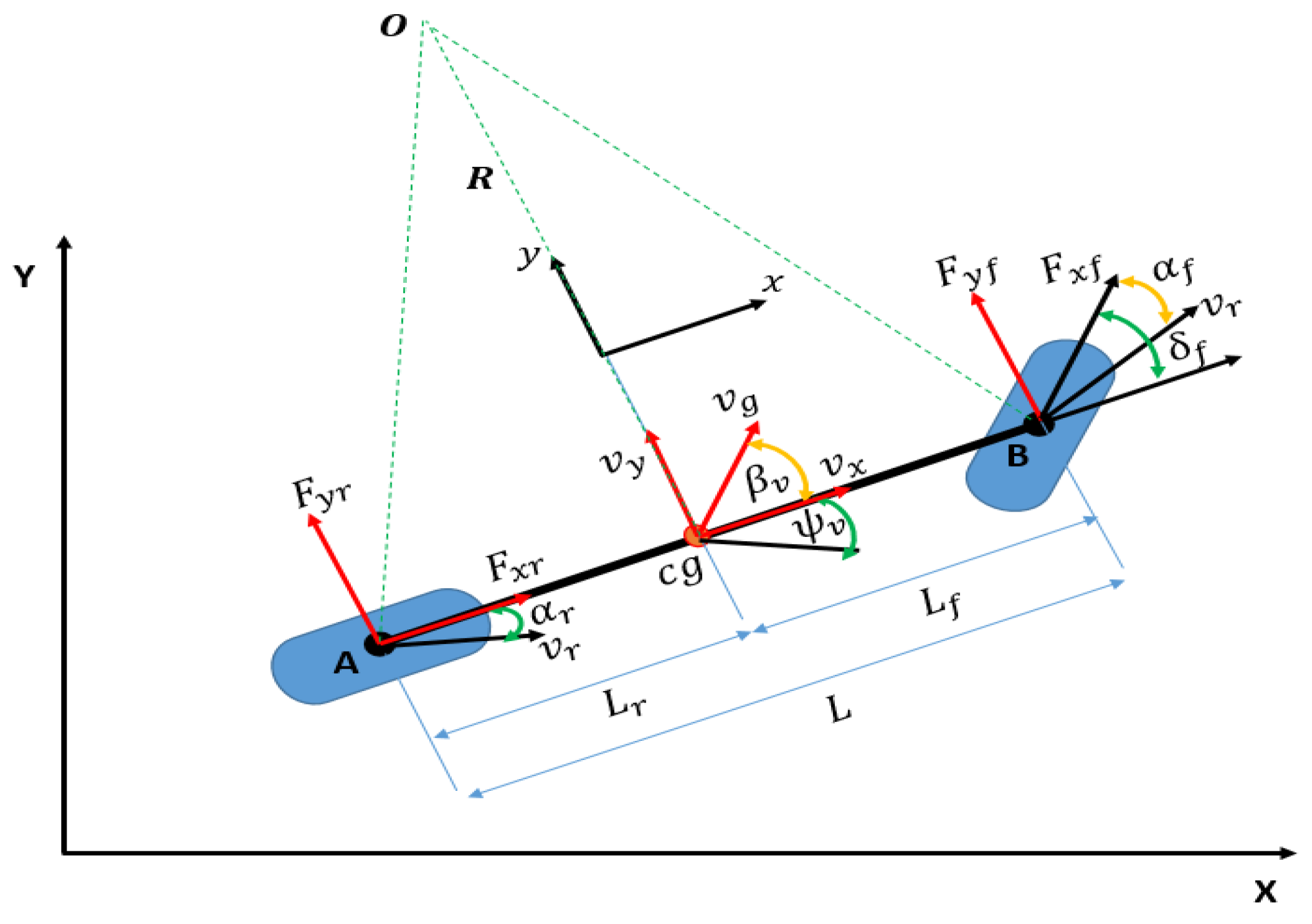
Figure 2.
Main Control Scheme.
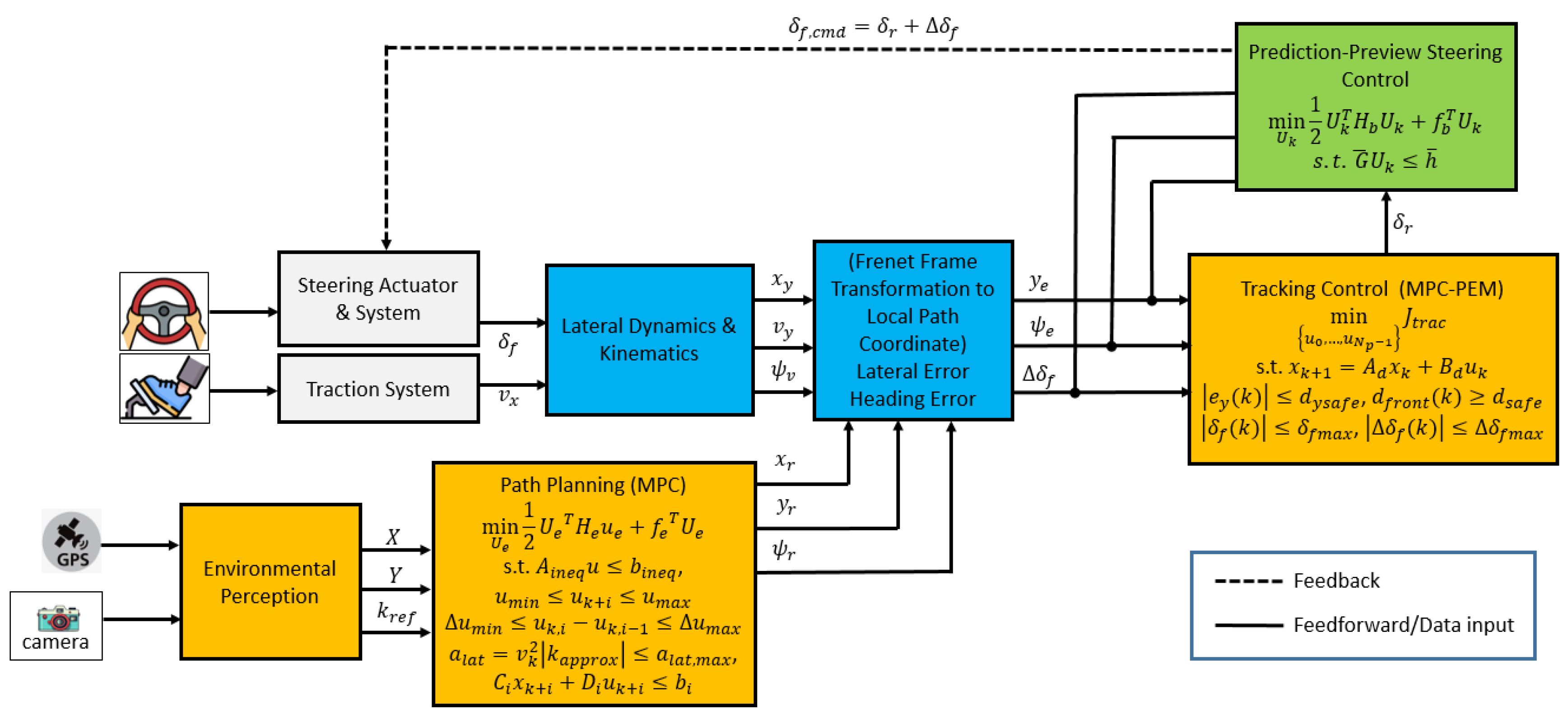
Figure 3.
Environmental sensor.
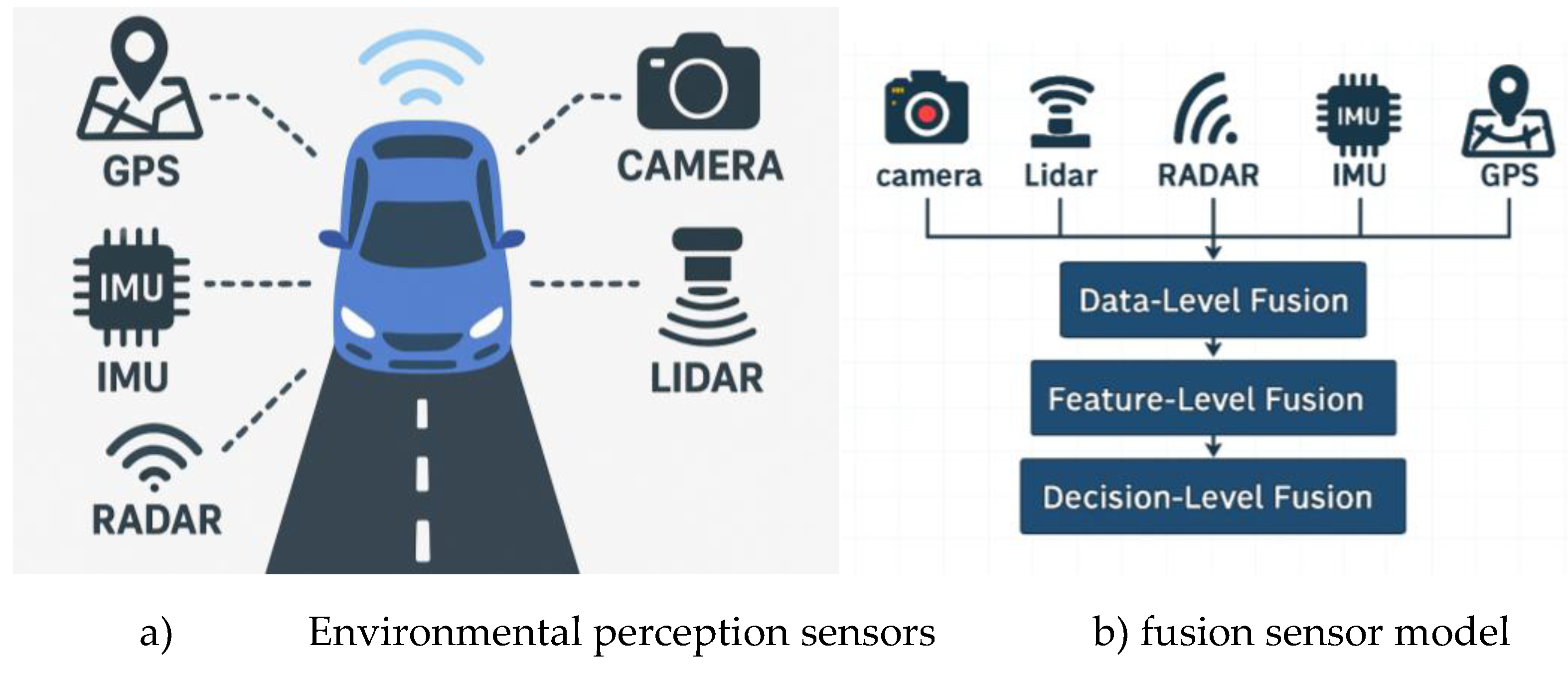
Figure 4.
Tracking Control Region.

Figure 5.
Reference Trajectory based on GPS Data.
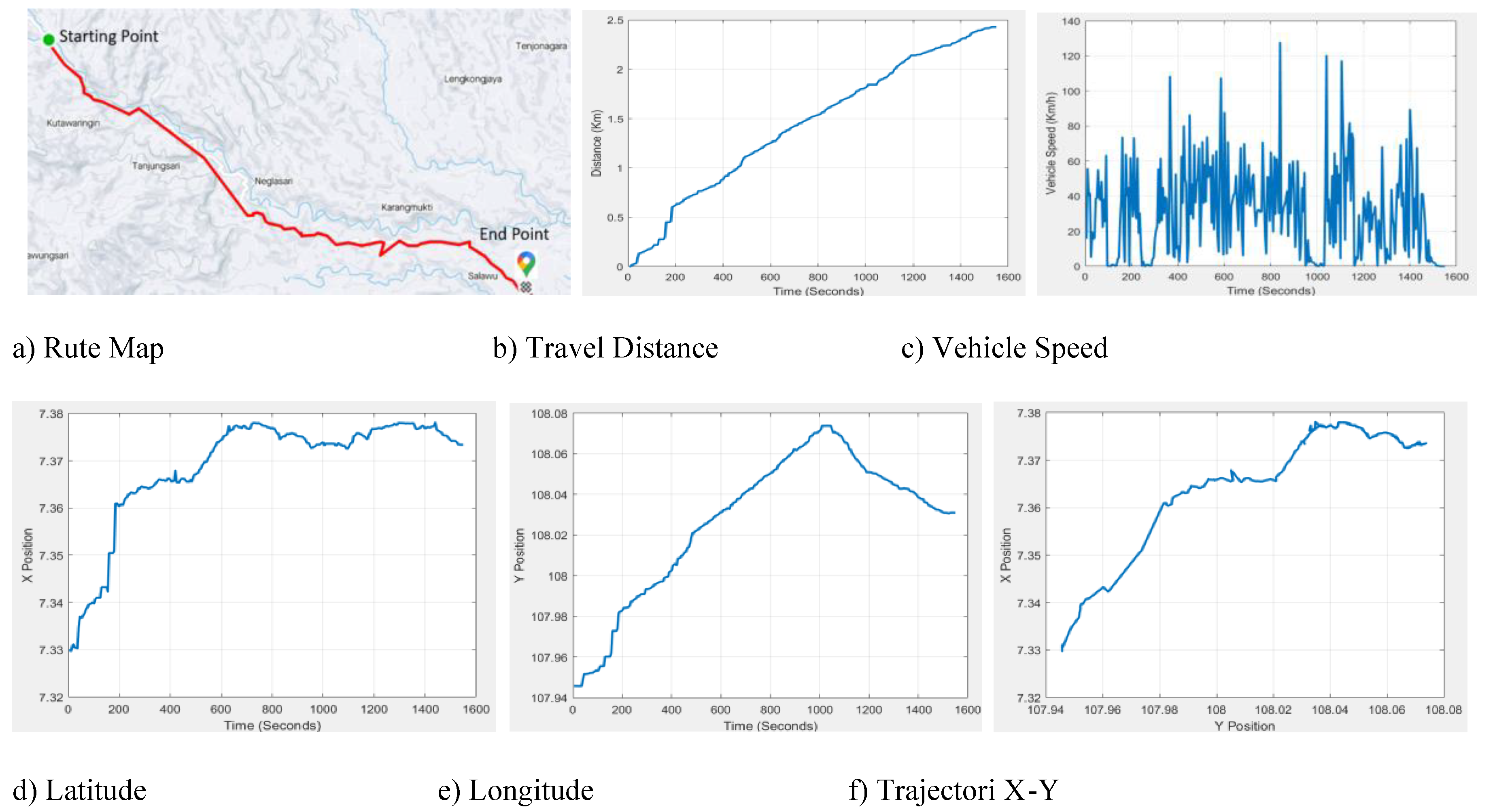
Figure 6.
Camera Sensing and Image Processing.
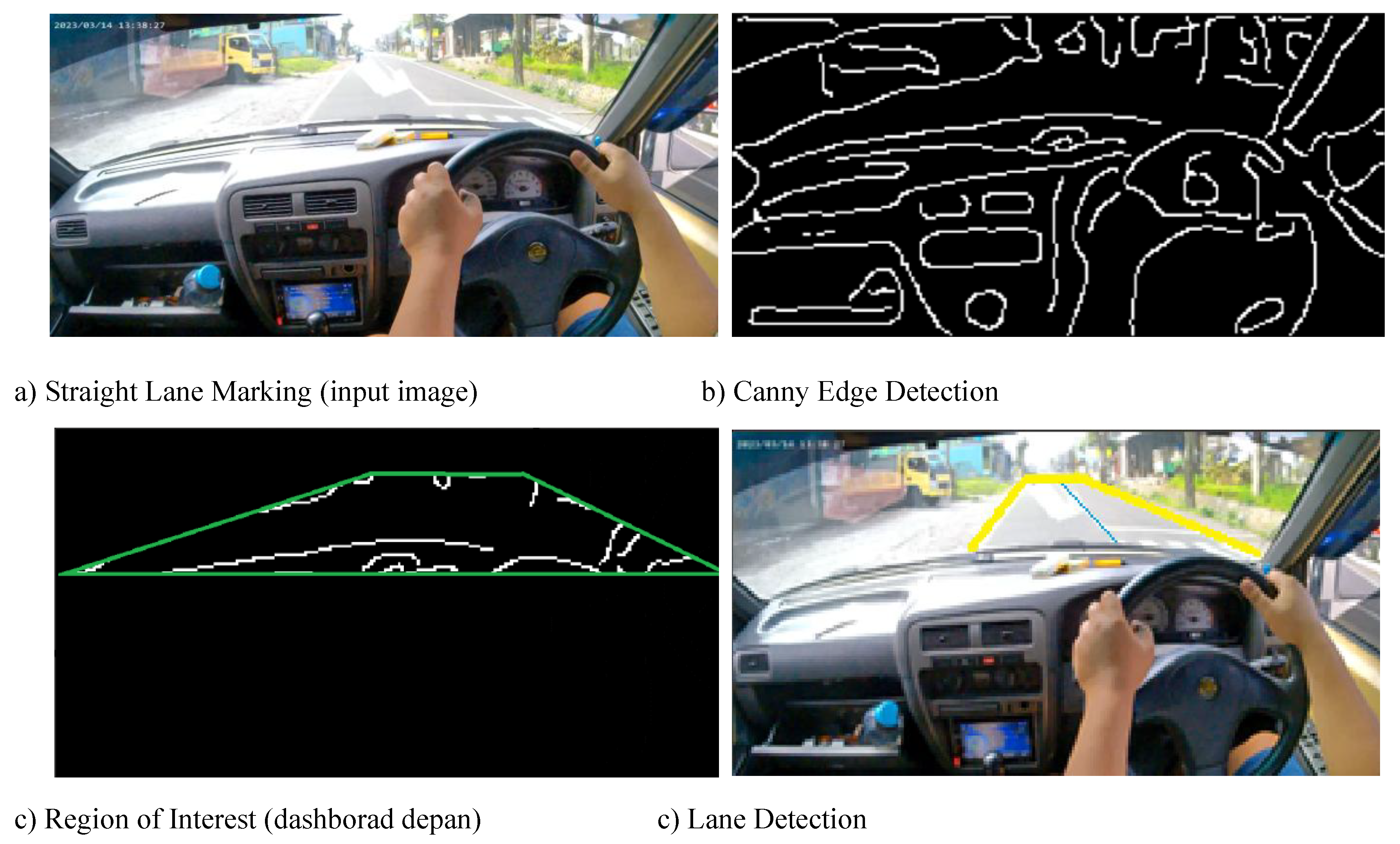
Figure 7.
Path Planning Based on GPS Data.
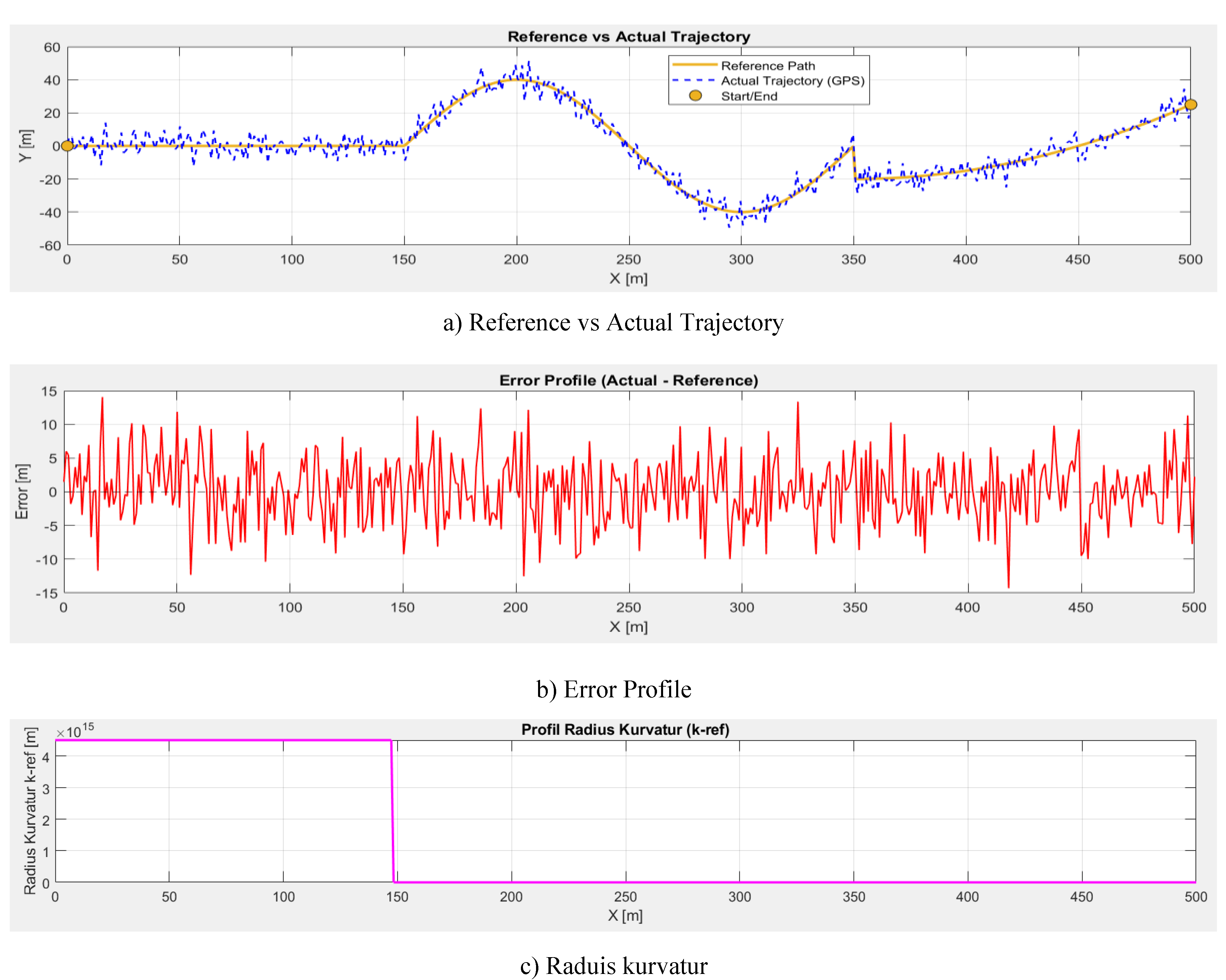
Figure 8.
Path Planning with MPC.
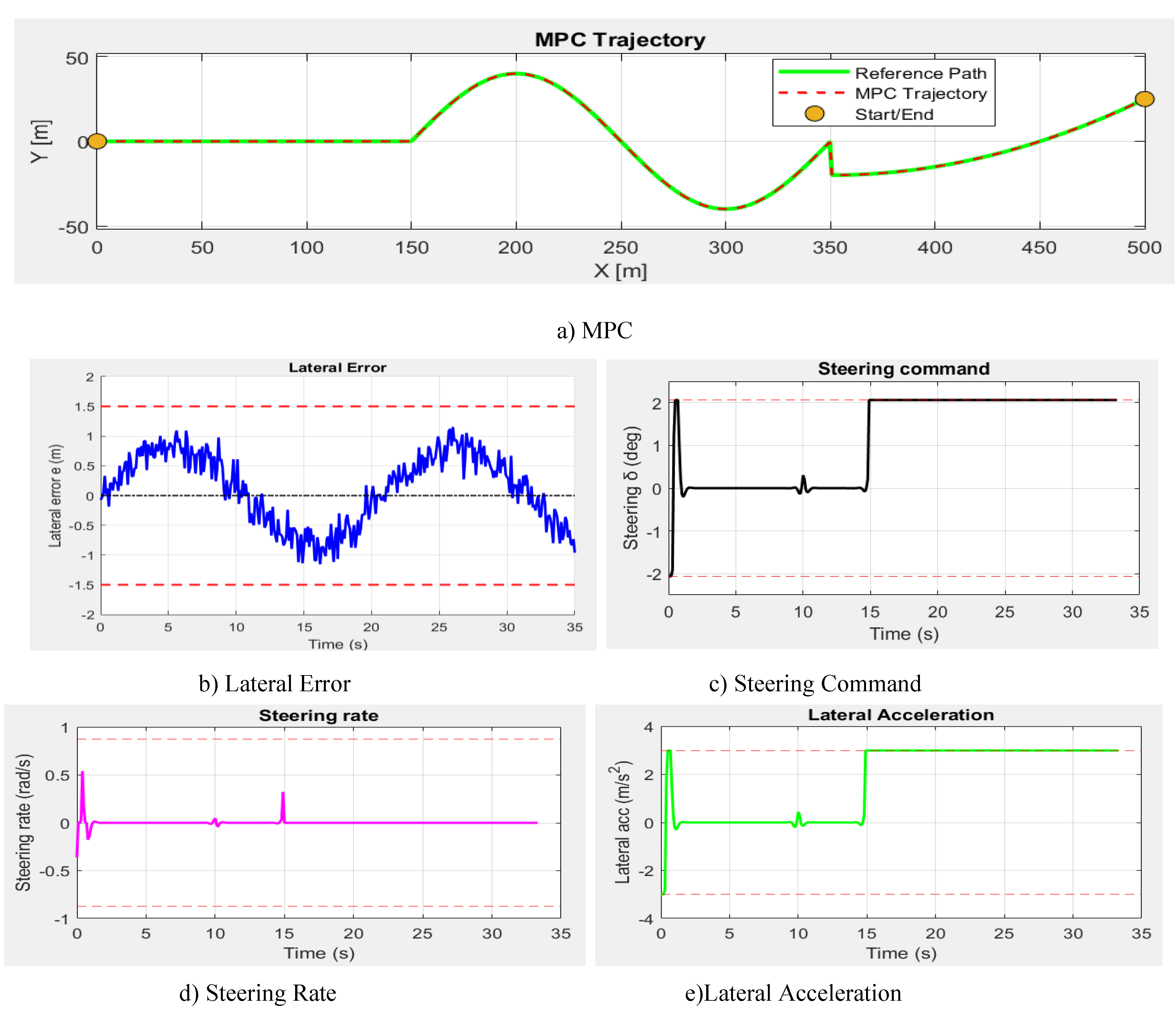
Figure 9.
Tracking Control with MPC + PEM.
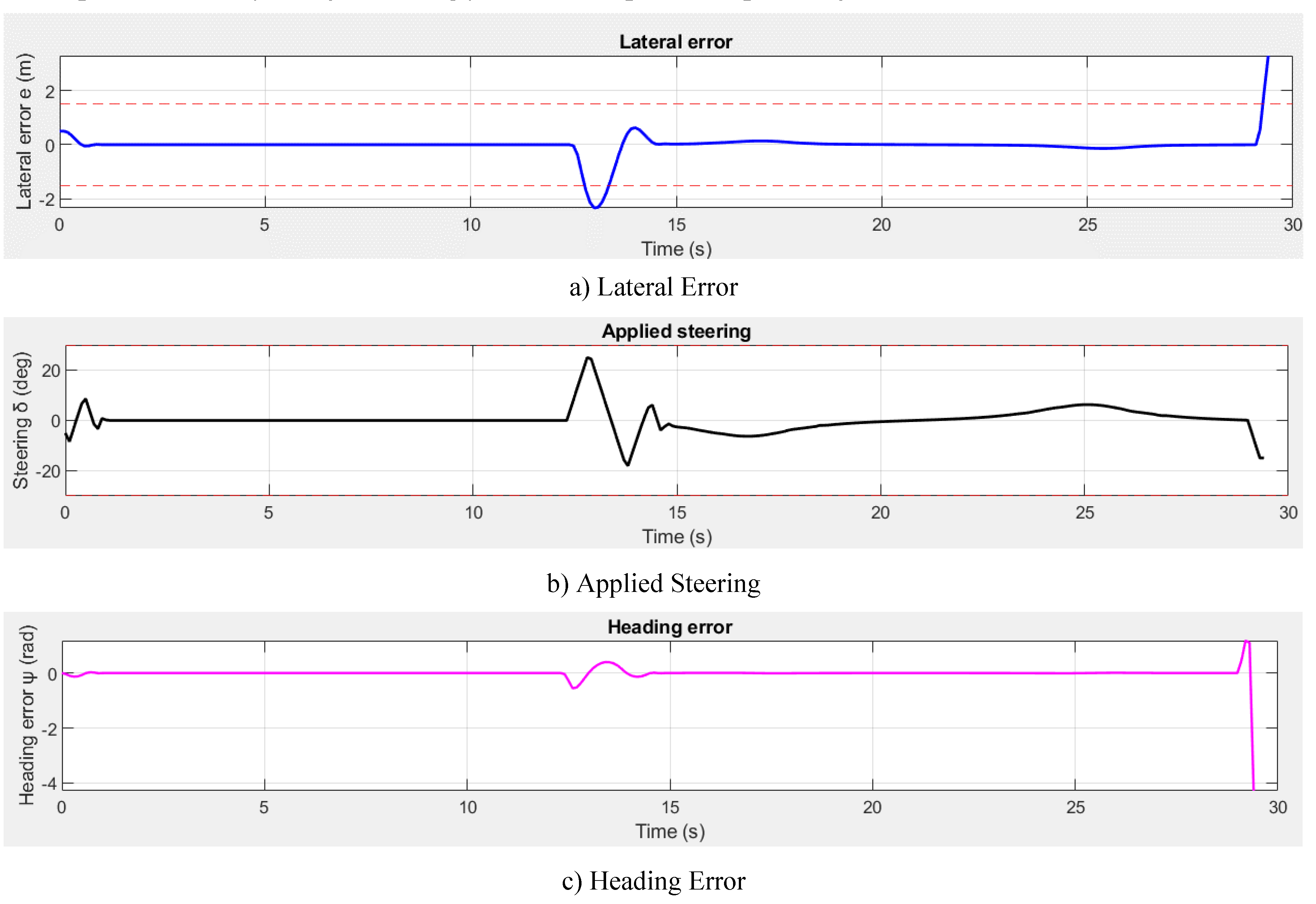
Figure 10.
Tracking Control Comparison.
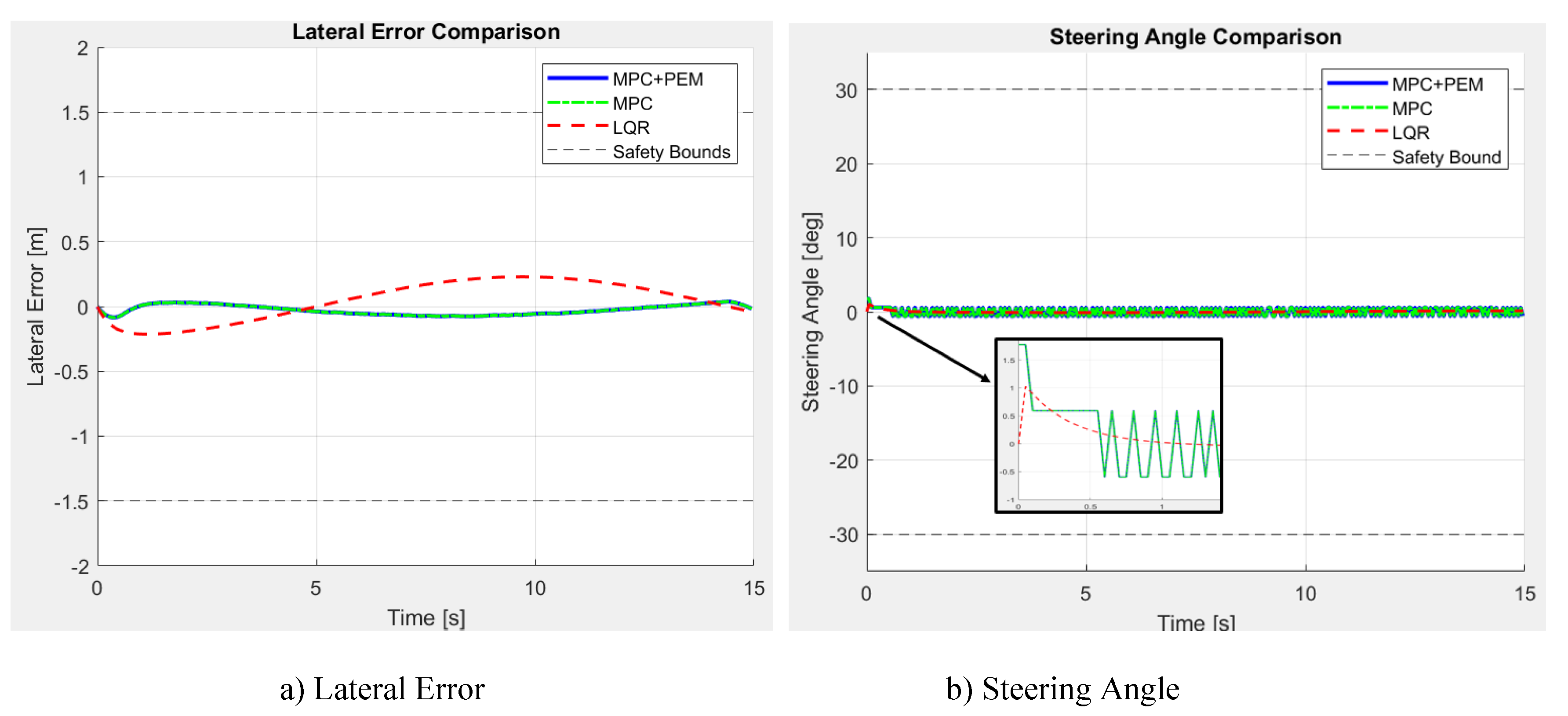
Figure 11.
Prediction-Preview Steering Control.
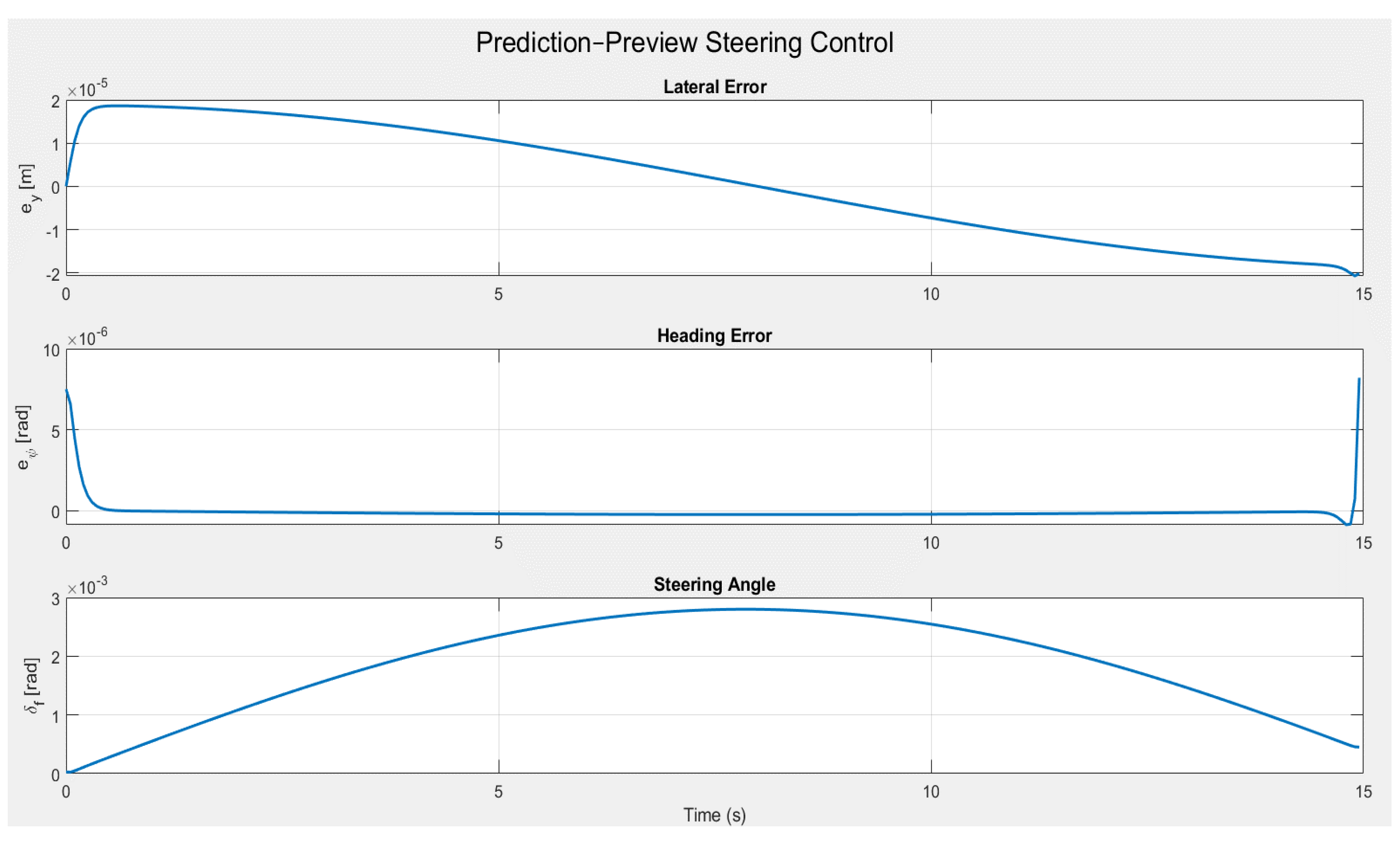
Figure 12.
Prediction-Preview Steering Control Comparison.
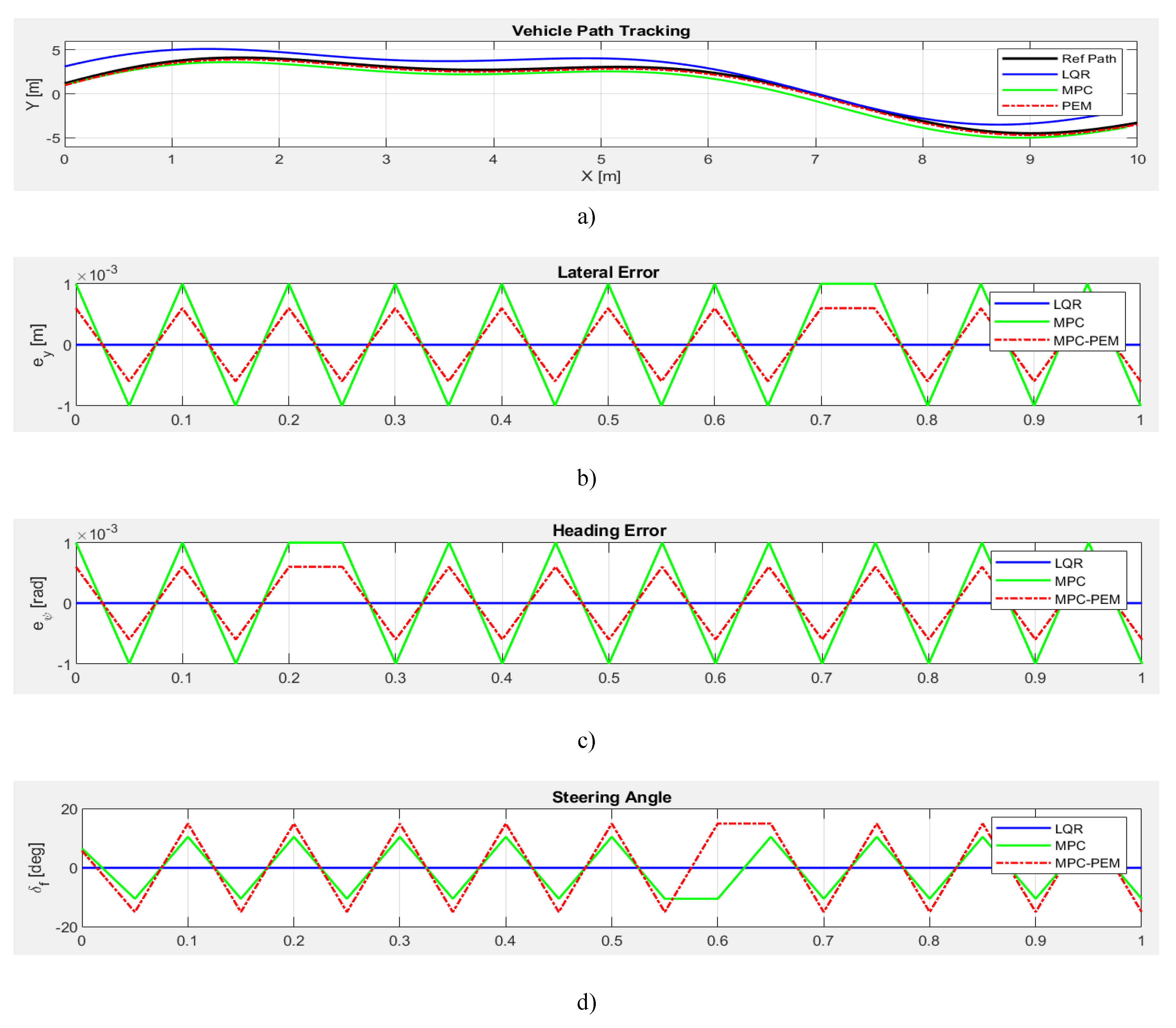

Table 1.
Comparison of Control Methods for Vehicle Path Tracking System Performance.
| Method | Rate Error Lateral (m) | Steering rate Error RMS | Cost Function | Max Steering Angle (0) | Deviation Steering Angle (0/s) | Rate Heading error (0) |
| MPC-PEM | 0.08 | 0.72 | 0.95 | 24.6 | 17.2 | 0.38 |
| MPC | 0.15 | 1.68 | 1.87 | 27.8 | 21.3 | 1.25 |
| LQR | 0.00 | 0.00 | 0.00 | 0.00 | 0.00 | 0.00 |
Table 2.
Performance and Accuracy Test.
| Method | Lateral Error (m) 10-4 | Heading Error (rad) 10-4 | Steering Angle (0) | Deviation Steering Angle(0/s) | ||||||
| Max | RMSE | IAE | Max | RMSE | IAE | RMSE | IAE | |||
| LQR | 8.5 | 9.7 | 7.2 | 7.9 | 8.5 | 6.4 | ±12.4 | 1.52 | 0.85 | 0.936 |
| MPC | 6.7 | 7.9 | 6.1 | 5.9 | 6.8 | 5.5 | ±14.2 | 1.08 | 1.10 | 0.674 |
| MPC-PEM | 4.3 | 5.3 | 4.2 | 3.8 | 4.9 | 3.7 | ±13.7 | 0.86 | 0.95 | 0.492 |
Disclaimer/Publisher’s Note: The statements, opinions and data contained in all publications are solely those of the individual author(s) and contributor(s) and not of MDPI and/or the editor(s). MDPI and/or the editor(s) disclaim responsibility for any injury to people or property resulting from any ideas, methods, instructions or products referred to in the content. |
© 2026 by the authors. Licensee MDPI, Basel, Switzerland. This article is an open access article distributed under the terms and conditions of the Creative Commons Attribution (CC BY) license (http://creativecommons.org/licenses/by/4.0/).
Copyright: This open access article is published under a Creative Commons CC BY 4.0 license, which permit the free download, distribution, and reuse, provided that the author and preprint are cited in any reuse.


