
Submitted:
31 July 2025
Posted:
01 August 2025
You are already at the latest version
Abstract
Path tracking is a fundamental challenge in the development of automated driving systems, requiring precise control of vehicle motion while ensuring smooth and stable actuation signals. Advancements in this field often lead to increasingly complex control solutions that demand significant computational effort and are difficult to parameterize. A novel variable structure path-tracking control approach, that is based on the geometrically optimal solution of a Dubins car, offers a promising solution to this challenge. The controller generates an n-smooth and differentially bounded steering angle and, with n+1 parameters, can be tuned towards performance, robustness or low magnitude of the steering angle derivatives. In prior work, this controller demonstrated its performance, robustness and tunablity in various simulations. In this contribution, we address the challenges of implementing this controller in a real vehicle, including system dead time, low sampling rates, and discontinuous paths. Key adaptations are proposed to ensure robust performance under these conditions. The controller is integrated into a comprehensive automated driving system, incorporating planning and velocity control, and evaluated during an overtaking maneuver (double-lane change) in a real-world setting. Experimental results demonstrate good reaching and tracking behavior despite significant disturbances, with smooth steering angle outputs. This work validates the controller's practical applicability and effectiveness, highlighting its potential for real-world automated driving applications.
Keywords:
Automated driving systems
; Path tracking
; robust control
; steering angle smoothness
; experimental validation
1. Introduction
One of the most pressing challenges in modern robotics is the navigation of autonomous vehicles, which requires the seamless integration of perception, planning, and control systems. A key task in this context is path tracking, which involves accurately following a predetermined trajectory while accounting for vehicle dynamics, environmental disturbances and system limitations.
Path tracking control for automated vehicles must reconcile two often competing demands: the need for mathematically sound control laws that guarantee stability, and the practical requirements of real-world vehicle dynamics where steering smoothness and computational feasibility are paramount. While the theoretical aspects of this challenge have been extensively studied [1,2,3,4], the transition from simulation to real-world implementation presents unique obstacles that are frequently underrepresented in the literature. Publications dealing with the real-world implementation of AD functions for cars and car-like vehicles are [5,6,7,8].
In our previous work [9], we established the theoretical foundations for a novel path tracking controller that combines:
- Geometric optimality through Dubins path principles
- -smooth steering outputs with bounded derivatives
- Systematic multi-objective tunability via parameters
- Global asymptotic convergence
These characteristics were achieved through an innovative approach involving a fictive trailer system, where a lead wheel follows a Dubins-optimal path and kinematic relations ensure a smooth steering angle for the actual vehicle. An alternative approach to this idea is in [10], who addressed the challenge of the discontinuous Dubins path with Krasovskiis principle.
While [9] comprehensively addressed the theoretical framework, this paper focuses on the critical next step: practical implementation and validation in real-world conditions. We identify and address three fundamental challenges that emerge when deploying the controller on actual vehicle hardware:
- Compensation of system dead-time
- Adapting to trajectory discontinuities
- Intuitive parameter tuning
Through extensive testing with a Ford Mondeo Hybrid test vehicle, we demonstrate how the theoretically sound controller can handle real-world conditions such as localization inaccuracy, actuator effects and computational constraints. Experimental results from a double-lane-change maneuver validate this approach, demonstrating consistent tracking errors of less than 0.3 m with passenger-comfort steering profiles, even in the presence of significant system delays and path discontinuities.
This work provides the crucial bridge between control theory and automotive practice, offering implementable solutions that preserve the original controller’s mathematical guarantees while meeting the rigorous demands of real-world vehicle operation.
2. Smooth and Robust Steering Controller
In [9] we presented a multi-objective path tracking control for car-like vehicles with differentially bounded n-smooth output. This control is shortly summarized in this section.
The controller is based on a sliding mode controller, which steers the vehicles axis along Dubins optimal curve.
Where is the path curvature and is the sliding surface, creating Dubins optimal path for reaching a straight reference path. e and are the control errors as visualized in Figure 1. The lateral error e is measured orthogonal to the reference path at and is the shortest distance between rear wheel and reference path. While is the maximum curvature the vehicle can reach, the sliding surface is designed to approach the reference path on a larger radius of curvature to introduce a control reserve and consequently obtain robustness to disturbances.
With kinematic relations, we could compute the steering angle such that the rear wheels of the vehicle follow the curvature . However, this steering angle would be discontinuous, as is . To obtain smoothness, we do not force the rear wheel to follow the Dubins curve, but the front wheel. The rear wheel is trailoring the front wheel asymptotically, with a smooth curvature and thus the vehicle has a smooth steering angle. This is illustrated in Figure 2.
To push this further, we introduce a fictive lead wheel that follows the Dubins curve. The front wheel follows with smooth curvature and the rear wheel follows with smooth change of curvature . We describe the vehicle, extened with the lead wheel, with the state vector containing the control error of the rear wheel and the steering angles:
Where is the fictive steering angle of the lead wheel. From kinematic trailor equations we get the relation between and the steering rate :
According to [9], the control law extended for the lead wheel is:
Where is the curvature of the lead wheel. This curvature relates to the steering rate of the lead wheel, and finally the steering acceleration:
Applying the steering acceleration (5b) to the steering system, the steering angle, steering rate and steering acceleration are bounded. We define the maximum curvature such that :
The bounds of the steering rate and steering acceleration are:
With , and .
In [9] a parameterization scheme is described. By specifying limits for the steering angle and rate (derivative in time) , the control parameters and are dynamically tuned.
3. Real Test Conditions
We apply the controller on a passenger vehicle: the Ford Mondeo fourth generation hybrid. It is equipped with a Dataspeed by-wire kit [11], providing a CAN interface to throttle, brake and a steering controller. The proposed controller is embedded in an automated driving stack that is shortly described in the next section. The section is followed by sections describing the steering system and vehicle localization.
The test is conducted on a two-lane testing ground comprising a straight road segment of approximately 170m, as shown in Figure 3.
3.1. AD System and Driving Maneuver
The AD system is designed for fully automated driving in urban environments. For testing the path tracking controller, we manually trigger a double-lane-change maneuver with constant velocity. The active components of the AD system are shown in Figure 4 and consist of a trajectory planner, a path tracking and a velocity tracking controller. It receives sensor data from a global positioning system described in Section 3.3 and outputs steering and throttle signals to the actuation system described in Section 3.2.
The trajectory planner creates a smooth path (a Catmull-Rom spline [12]) from one lane to the left lane and then back to the original lane. The path is shown in Figure 5. The path is continuous, meaning that the tangents change continuously along the path, while the curvature is discontinuous. The curvature reaches values of maximal .
The presented path tracking controller outputs the steering angle into the steering system. The actual control signal, the steering acceleration , acts as internal state to guarantee smoothness and bounded derivatives of .
The velocity controller is a PID control that outputs pedal positions of throttle and brake to the actuation system.
3.2. Steering System
The steering system consists of a controller that sets the steering torque such that the steering rod follows the target angle. The step response of the steering system is shown in Figure 6. After a dead-time of 80ms, the steering angle is reached at a rate of maximum rad/s. The response to a sine steering input is shown in Figure 7. The target steering angle is sampled at 50Hz.
3.3. Positioning System
Localisation is performed using an inertial navigation system (INS). This consists of the Novatel ProPak 6 GNSS receiver (Novatel, 2017), coupled with two antennas and an inertial Measurement Unit (IMU). Using the RTK (real-time kinematic positioning) method with IMU coupling, the GNSS receiver can achieve centimetre-level positioning accuracy and estimate the heading (the angle from true north). The INS is installed approximately on the rear axle. In a straight drive on the testing ground, the measured vehicle orientation differs from the vehicles driving direction (the tangent of the driven path) by rad. When computing the front axle error from the measured position, the orientation error leads to an error estimate of m.
3.4. System Integration
To connect the AD system with the steering system and the positioning system in the vehicle, we use the asynchronous high-performance platform RTMaps [13]. The sensor and actuator interfaces as well as the path tracking controller are implemented in C++ to minimize the processing time, achieving a result below 20ms. The INS outputs measurements at 100Hz, the path tracking controller and the actuation system operate at 50Hz. The processing time of the controller is 20ms and the sub-sampling of the actuation system produces delays of up to 45ms. The steering controller adds an additional delay of 150ms (the steering response in Figure 6 is simplified to an average delay). The delay of the INS is unknown. We will approximate the total delay by tuning the dead-time compensation for the optimal delay.
4. Controller Adpations
To make the controller applicable in the real test conditions, some adaptions are necessary, which are presented in this section.
4.1. Dead-Time Compensation
Due to delays in the actuation system, interfaces and components, there is a total dead-time of more than 150ms in the closed loop system. To compensate this, we apply the kinematic based prediction method presented in [14]. The structure is similar to the Smith predictor [15], but the estimated prediction vector is transformed by the measured orientation of the vehicle to compensate for divergence of the plant model and the real plant. The structure is shown in Figure 8. The state estimate follows the plant model:
Where is the rotation matrix, is the discrete time step, v is the longitudinal velocity and i is the index progressing in time .
According to [14] and as illustrated in Figure 8, the dead-time compensated vehicle state (the output of the dead-time compensator) is the delayed (measured) vehicle state plus the state prediction based on the estimated state :
Where k relates to the dead-time . This predicted state is used to compute e and for the control law in equation (4). The dead-time compensation achieved best results with a compensation of .
4.2. Look-Ahead Distance
With dead-time compensation, the controller can react to disturbances and changes in path geometry in time. However, if the path geometry does not satisfy the continuity constraints resulting from the steering constraints (i.e. if the path does not have continuous, bounded curvature or changes in curvature), the vehicle will still be unable to follow the path. To improve tracking behaviour for discontinuities in paths, we introduce a look-ahead. The effect of this is shown in Figure 9 for an example of a path with a discontinuous orientation. Without look-ahead, the controller only responds to changes in path orientation once the vehicle has reached the edge of the path. With look-ahead, however, the controller reacts earlier, creating a path with low or no overshoot.
The lookahead distance is a constant value measured along the reference path. From the new reference position the control error e and are computed as before. This is illustrated in Figure 10. A look-ahead distance of 4m has been determined empirically for the present application.
5. Parameter Tuning and Test Results
Test drives are conducted in the real vehicle to determine the appropriate values for the three free parameters:
- The dead-time to be compensated : Rather than determining the actual dead time in system tests, we conduct tests to directly determine the optimal time estimate for compensating for dead time.
- The look-ahead distance : The optimal distance depends on the geometry of the reference path and is therefore determined in a representative maneuver.
- The maximum steering acceleration : To increase smoothness, the steering acceleration can be limited at the cost of control performance. While a theoretical optimum has been discussed in [9], robustness to model parameters proves to be more relevant in reality.
5.1. Compensated Dead-Time
The controller is evaluated on a straight reference path, with the steering signal only compensating for disturbances. When the dead-time is not estimated correctly, constant oscillations will occur. In Figure 11 the result of two test drives is shown. While the steering rate oscillates in both cases, with a correct estimate of the dead-time (), the oscillations in the steering angle and tracking error are significantly reduced. Note that the tracking error is unequal to zero, because of the error in orientation measurement, as discussed in Section 3.3.
5.2. Look-Ahead Distance
The lane change maneuver involves a jump in the curvature of the reference path. To react on this on time, a look-ahead distance is required. When the value is chosen too large, the controller is cutting corners, while a value too small leads to overshooting and can even destabilize the controller. In Figure 12, a test drive of a lane-change maneuver with and without look-ahead is shown. Without lookahead, the controller only reacts to the lane-change when the reference path has already changed. The first change of curvature leads to a control error such that the second change of curvature (back to straight on the new lane) creates a saturation of the steering angle and an even larger overshooting of the vehicle, as shown in Figure 13. With lookahead, the controller reacts 3s ahead in time, resulting in a small cutting corners effect of m and an overshoot below m.
5.3. Maximum Steering Acceleration
As is visible in Figure 11 and Figure 13, even though the dead-time is optimally compensated, there are still oscillations in the steering angle. While this does not impair the tracking error, the comfort and driver acceptance is significantly reduced. To solve this problem, we significantly increase the maximum steering acceleration.
5.4. Final Tests
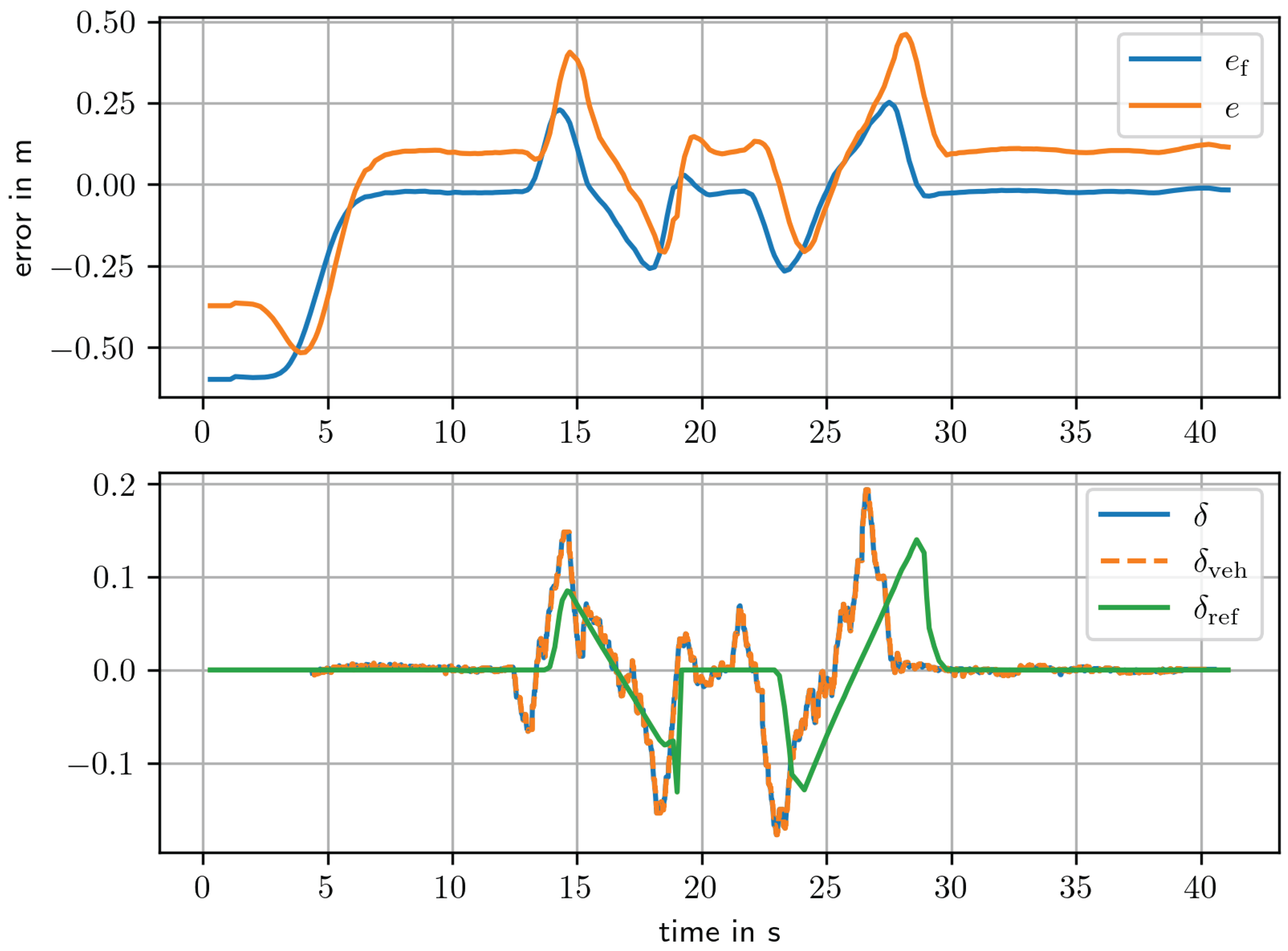
For the final test, the vehicle is manually positioned close to the reference path, the AD system is activated and the double lane change maneuver manually triggered. The results of the double lane-change maneuver are shown in Figure 14. The vehicle starts with an initial offset of approximately m from the path, approaching it with the front wheel. Within seconds (approximately m), without overshooting. During the lane change, the front wheel reaches a maximum error of m. Throughout the test, the steering angle remains well below its maximum, while the steering rate reaches its maximum of deg/s multiple times.
Due to the dead-time compensation and look-ahead, the steering angle leads the reference paths curvature, and the corresponding reference steering angle, . It is also interesting to note that the profile of the reference steering angle differs from the reference curvature shown in Figure 14 due to the linear approximation of the polynomial curve. The steering rate remains within the specified range except for the initial value. The actual initial steering angle is not known to the controller, so it is set to the desired value. This occurs immediately and at one other point in time, which may be the result of numeric errors due to discrete time differentiation.
5.5. Discussion and Conclusion
In [16] the concept of a robust controller based on Dubins optimal path has been theoretically analyzed. In [9], this controller has been extended to fit for real-world application in a car-like vehicle. By introducing continuity and constraints of the steering signal, the controller not only becomes applicable, but also tunable regarding comfort, tracking behavior and robustness at different velocities.
In this present work, real-world validation is conducted by integrating the controller into an AD system. However, important aspects have still not been handled. Real vehicle tests show that dead-time in the control loop leads to significant oscillations in the steering signal and thus the vehicle path. The vehicle reacts on discontinuous changes in the reference path too late, causing unnecessary overshoot.
By adding dead-time compensation and a lookahead distance, these problems can be overcome. Each feature comes with one parameter, that are tuned once, based on simple driving tests and seem to fit well for all subsequent driving tests. While the smooth steering angle is necessary to overcome chattering effect in the steering signal, tests showed that limiting the steering acceleration leads to low-frequency oscillations in the steering signal that indeed do not impair the tracking behavior, but decrease the driver acceptance. By setting the steering acceleration limit to large values, the steering behavior looks more usual.
Finally, after tuning 3 intuitive parameters (dead-time, lookahead, steering acceleration), the controller with smooth steering angle and dead-time compensation successfully performs the double-lane-change maneuver despite disturbances such as steering delays and pose measurement errors.
This work bridges theory and practice by demonstrating how a theoretically sound controller can be adapted to meet real-world demands. The solutions presented—dead-time compensation, look-ahead path sampling, and practical tuning—provide a blueprint for deploying advanced control algorithms on production vehicles while preserving stability and comfort. As autonomous systems advance, such translational efforts will be critical to achieving reliable, large-scale deployment.
Acknowledgments
This work was supported by the project Cynergy4MIE (Grant Agreement Nr. 101140226), which is Co-funded by the European Union. The projects are supported by the Chips Joint Undertaking and its members including top-up funding by the program “Digitale Technologien” of the Austrian Federal Ministry for Climate Action (BMK). The publication was written at Virtual Vehicle Research GmbH in Graz and partially funded within the COMET K2 Competence Centers for Excellent Technologies from the Austrian Federal Ministry for Climate Action (BMK), the Austrian Federal Ministry for Labour and Economy (BMAW), the Province of Styria (Dept. 12) and the Styrian Business Promotion Agency (SFG). The Austrian Research Promotion Agency (FFG) has been authorised for the programme management. Views and opinions expressed are however those of the author(s) only and do not necessarily reflect those of the European Union Key Digital Technologies Joint Undertaking. Neither the European Union nor the granting authority can be held responsible for them.
Abbreviations
The following abbreviations are used in this manuscript:
| AD | Automated Driving |
| CAN | Control Area Network |
| GNSS | Global Navigation Satellite System |
| IMU | Inertial Measurement Unit |
| INS | Inertial Navigation System |
| RTK | Real-Time Kinematic |
| PID | Proportional-Integral-Derivative |
References
- Ruslan, N.A.I.; Amer, N.H.; Hudha, K.; Kadir, Z.A.; Ishak, S.A.F.M.; Dardin, S.M.F.S. Modelling and control strategies in path tracking control for autonomous tracked vehicles: A review of state of the art and challenges. Journal of Terramechanics 2023, 105, 67–79. [Google Scholar] [CrossRef]
- Paden, B.; Cap, M.; Yong, S.Z.; Yershov, D.; Frazzoli, E. A Survey of Motion Planning and Control Techniques for Self-driving Urban Vehicles. IEEE Transactions on Intelligent Vehicles 2016, 1, 33–55. [Google Scholar] [CrossRef]
- Dominguez, S.; Ali, A.; Garcia, G.; Martinet, P. Comparison of lateral controllers for autonomous vehicle: Experimental results. In Proceedings of the IEEE Conference on Intelligent Transportation Systems, Proceedings, ITSC, 2016, pp. 1418–1423. [CrossRef]
- Yao, Q.; Tian, Y.; Wang, Q.; Wang, S. Control Strategies on Path Tracking for Autonomous Vehicle: State of the Art and Future Challenges. IEEE Access 2020, 8, 161211–161222. [Google Scholar] [CrossRef]
- Zhou, Y.; Wang, Z.; Panchal, J.H.; Mahmoudian, N. Design and Deployment of a real-world autonomous driving test platform 2024. [CrossRef]
- Xu, S.; Peng, H. Design, Analysis, and Experiments of Preview Path Tracking Control for Autonomous Vehicles. IEEE Transactions on Intelligent Transportation Systems 2020, 21, 48–58. [Google Scholar] [CrossRef]
- Han, X.Z.; Kim, H.J.; Kim, J.Y.; Yi, S.Y.; Moon, H.C.; Kim, J.H.; Kim, Y.J. Path-tracking simulation and field tests for an auto-guidance tillage tractor for a paddy field. Computers and Electronics in Agriculture 2015, 112, 161–171. [Google Scholar] [CrossRef]
- Takanezawa, K.; Ozaki, R.; Takesue, N.; Hiruma, J.; Mikado, J. Four-Wheel Independent Steering and Four-Wheel Independent Driving Robot and its Simultaneous Path and Orientation Tracking Control. International Journal of Automation Technology 2025, 19, 521–534. [Google Scholar] [CrossRef]
- Festl, K.; Stolz, M.; Watzenig, D. Multi-objective path tracking control for car-like vehicles with differentially bounded n-smooth output. IEEE Transactions on Intelligent Transportation Systems 2024, 25, 8017–8027. [Google Scholar] [CrossRef]
- Marigo, A.; Piccoli, B. Safety controls and applications to the Dubins’ car. Nonlinear Differential Equations and Applications 2004, 11, 73–94. [Google Scholar] [CrossRef]
- DATASPEEDInc.. Dataspeed by-wire Kit, 2025.
- Catmull, E.; Rom, R. A CLASS OF LOCAL INTERPOLATING SPLINES. In Computer Aided Geometric Design; Academic Press, 1974; pp. 317–326. [CrossRef]
- Intempora. Intempora.com, 2018.
- Festl, K.; Stolz, M. A nonlinear dead-time compensation method for path tracking control. In (to be published) Recent advances in autonomous vehicle technology - perception and path planning; Springer, 2025.
- Normey-Rico, J.E.; Camacho, E.F. Control of dead-time processes; Springer International Publishing, 2007; pp. 1–462. [CrossRef]
- Tieber, K.; Rumetshofer, J.; Stolz, M.; Watzenig, D. Sub-optimal and robust path tracking: a geometric approach. In Proceedings of the 2021 IEEE/RSJ International Conference on Intelligent Robots and Systems (IROS), 2021, pp. 8381–8387.
Figure 1.
For the simple tracking problem, the vehicle reference point p is in the rear axle of the vehicle, the control error e is the shortest distance to the reference path and the control signal is the vehicle path curvature .
Figure 1.
For the simple tracking problem, the vehicle reference point p is in the rear axle of the vehicle, the control error e is the shortest distance to the reference path and the control signal is the vehicle path curvature .
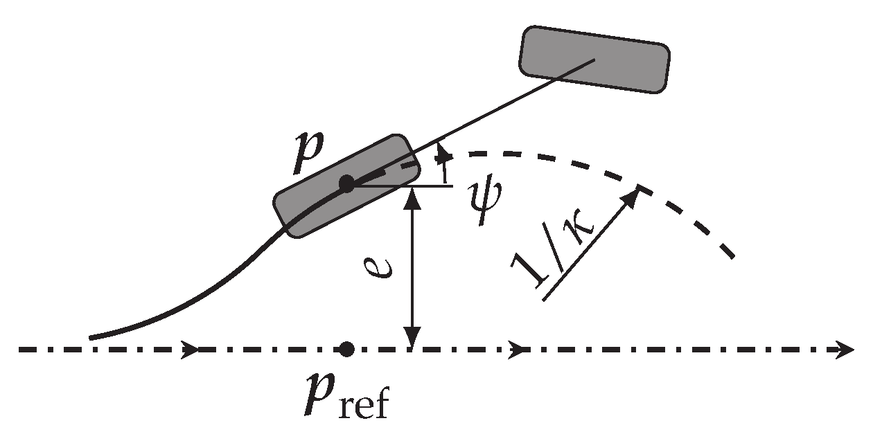
Figure 2.
For the single track model, the path tracking error can be measured in the rear wheel and the front wheel .
Figure 2.
For the single track model, the path tracking error can be measured in the rear wheel and the front wheel .
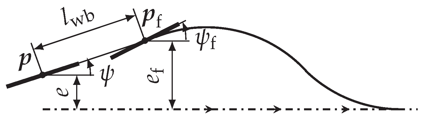
Figure 3.
The Ford Mondeo test vehicle on the testing ground.
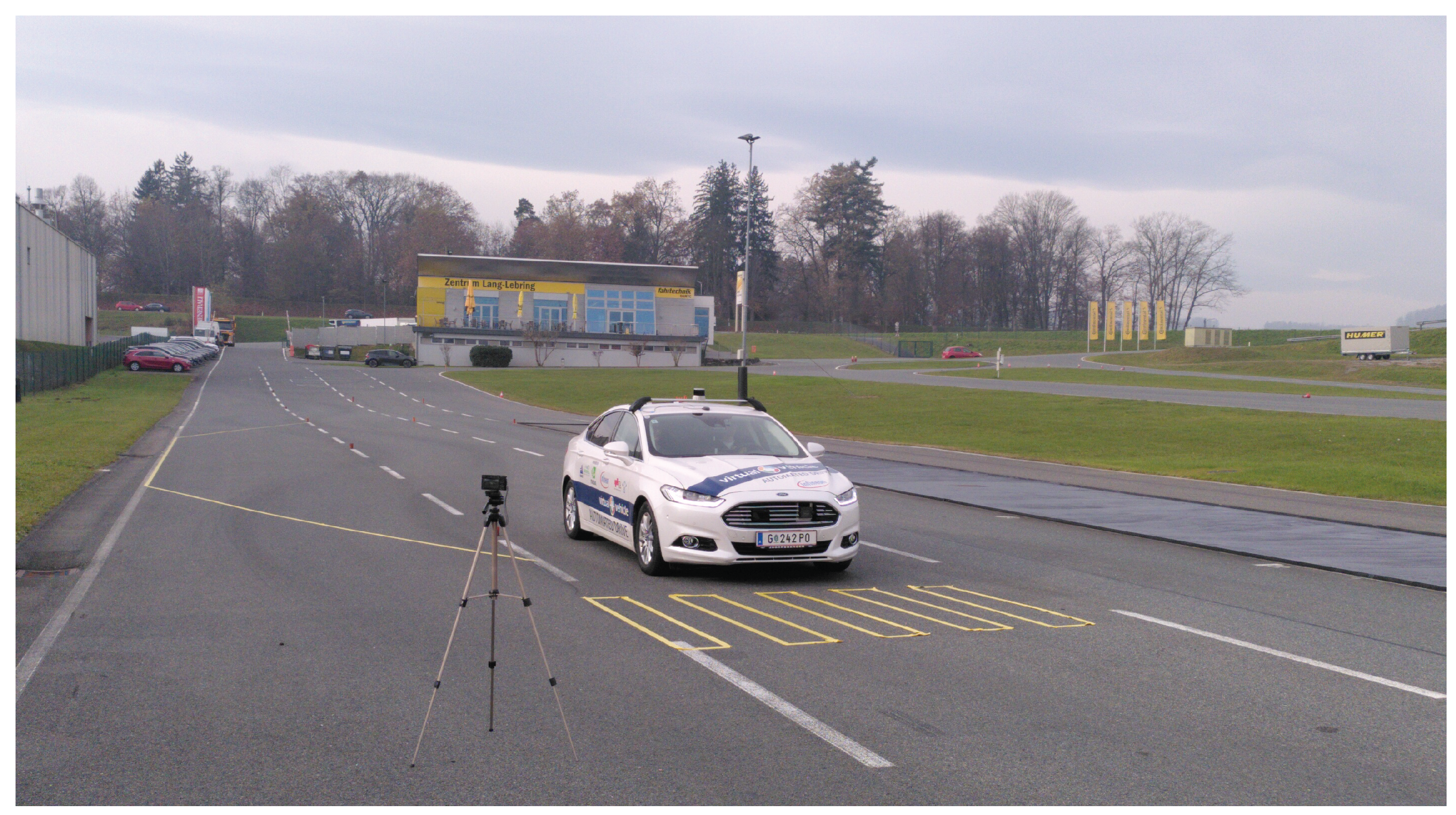
Figure 4.
AD system in which the path tracking controller is embedded.
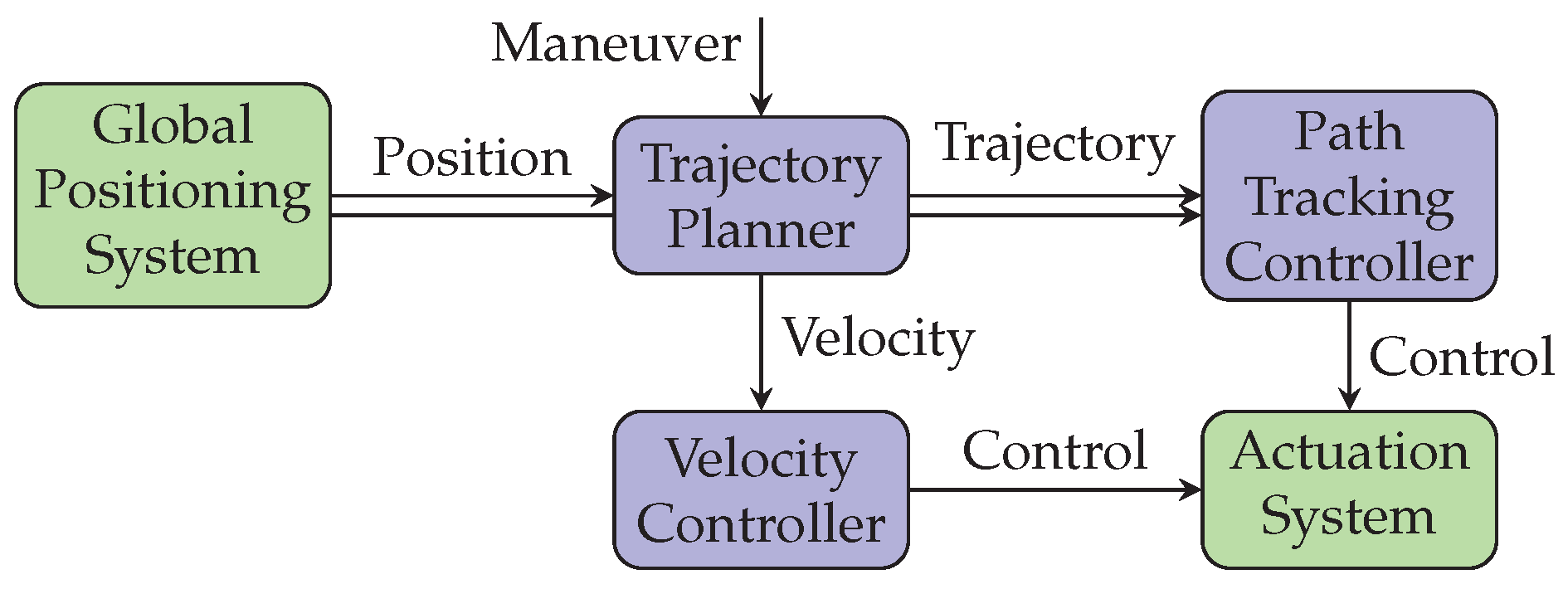
Figure 5.
Double lane change maneuver.
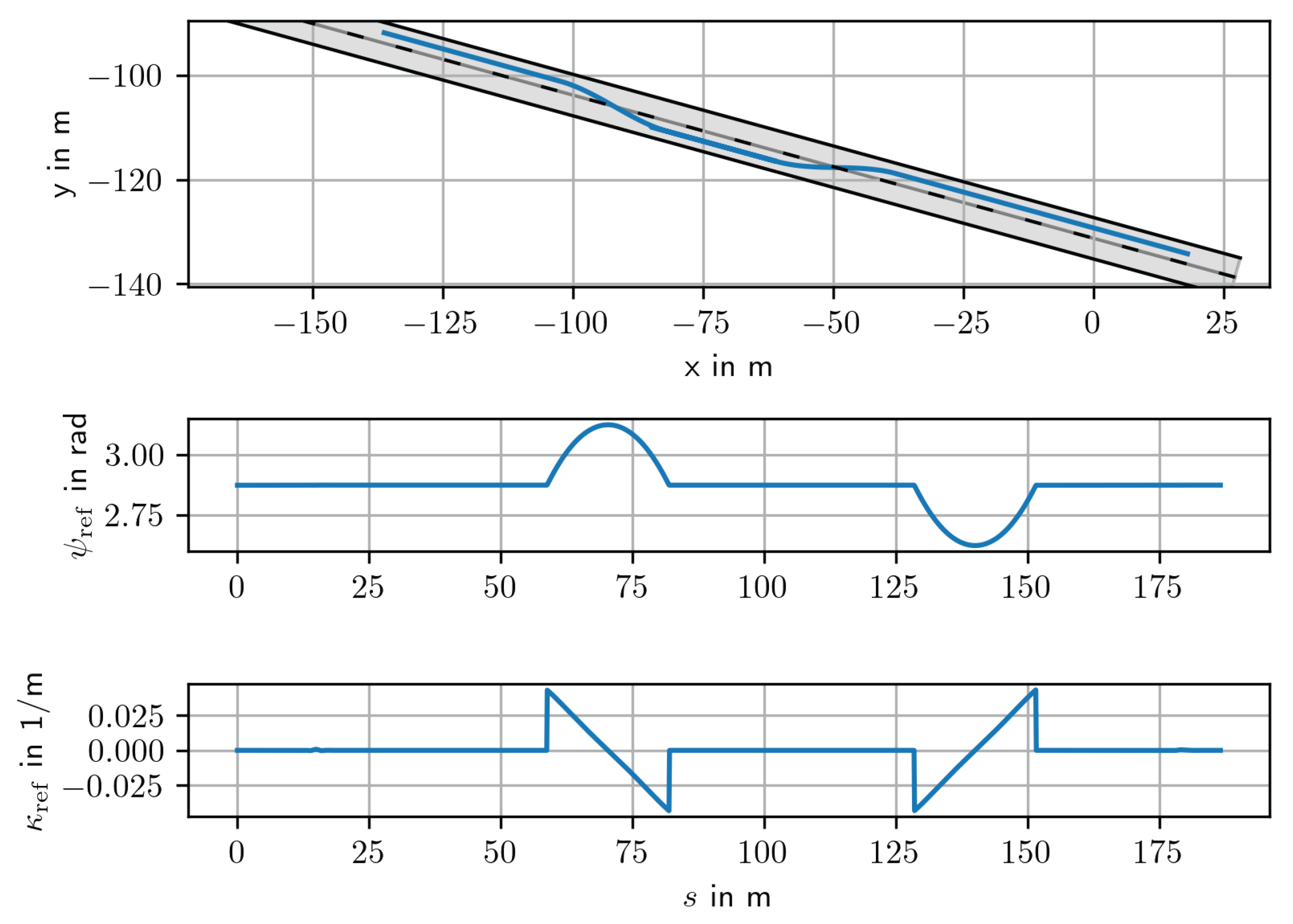
Figure 6.
Step response of the steering model which is implemented as a constant dead-time and a third order low pass.
Figure 6.
Step response of the steering model which is implemented as a constant dead-time and a third order low pass.
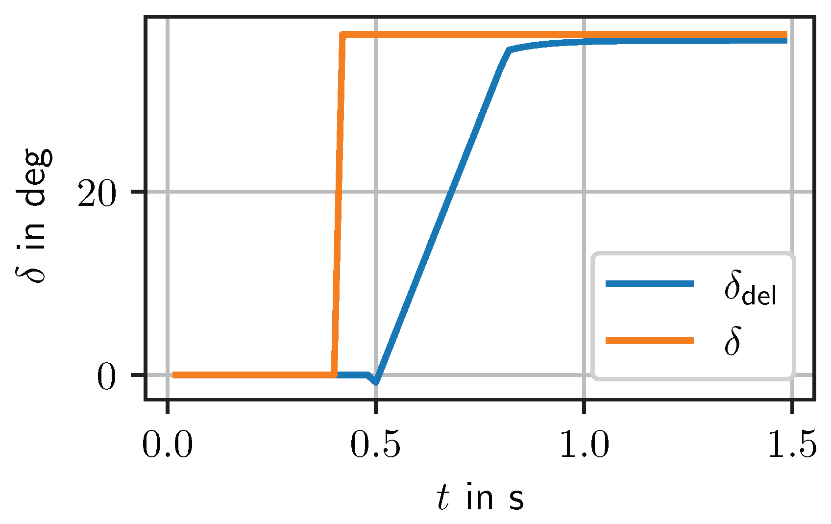
Figure 7.
Sine response of the steering system and torque on the steering rod.
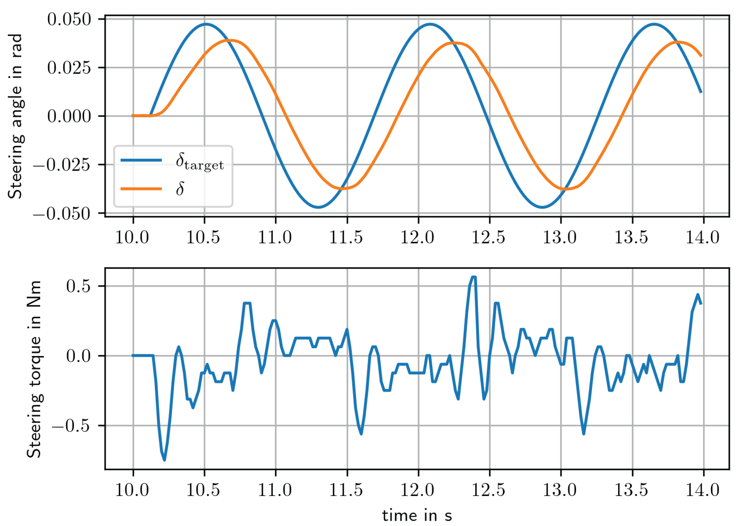
Figure 8.
Structure of the control system with a delayed plant and dead-time compensation with a prediction plant model.
Figure 8.
Structure of the control system with a delayed plant and dead-time compensation with a prediction plant model.
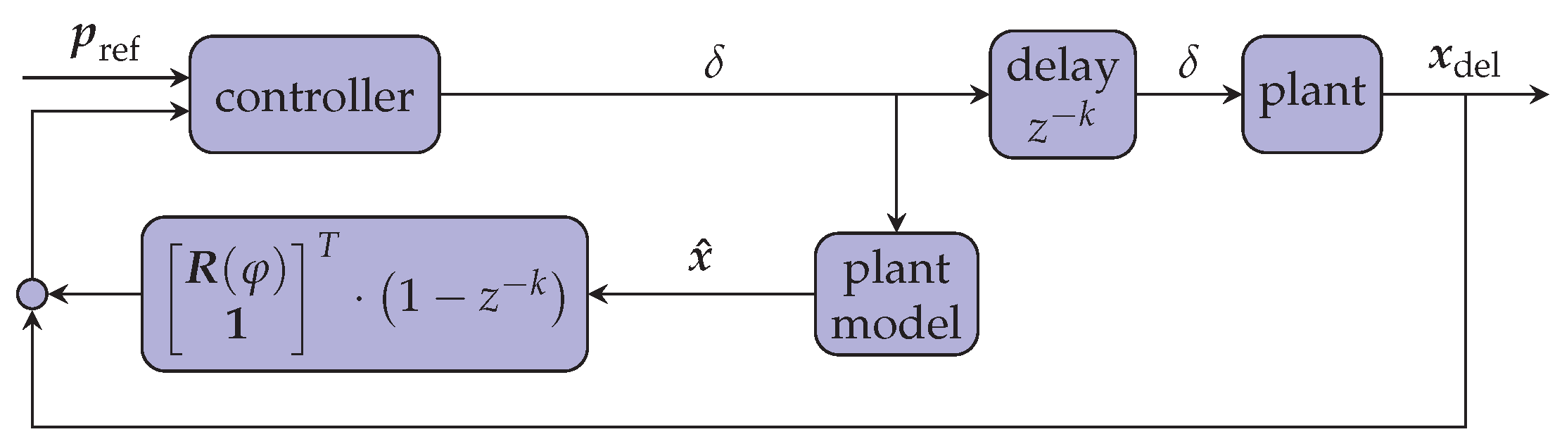
Figure 9.
Tracking a discontinuous reference path without look ahead and with look ahead of different magnitude.
Figure 9.
Tracking a discontinuous reference path without look ahead and with look ahead of different magnitude.
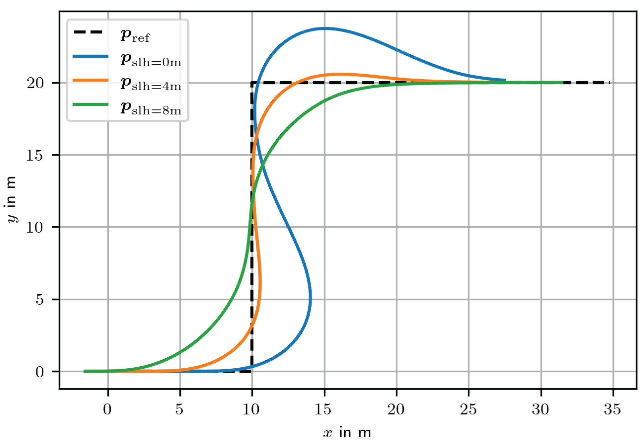
Figure 10.
Lateral error e with a look ahead distance .
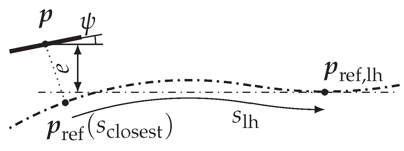
Figure 11.
Tracking a straight reference path with dead-time estimated properly or underestimated.
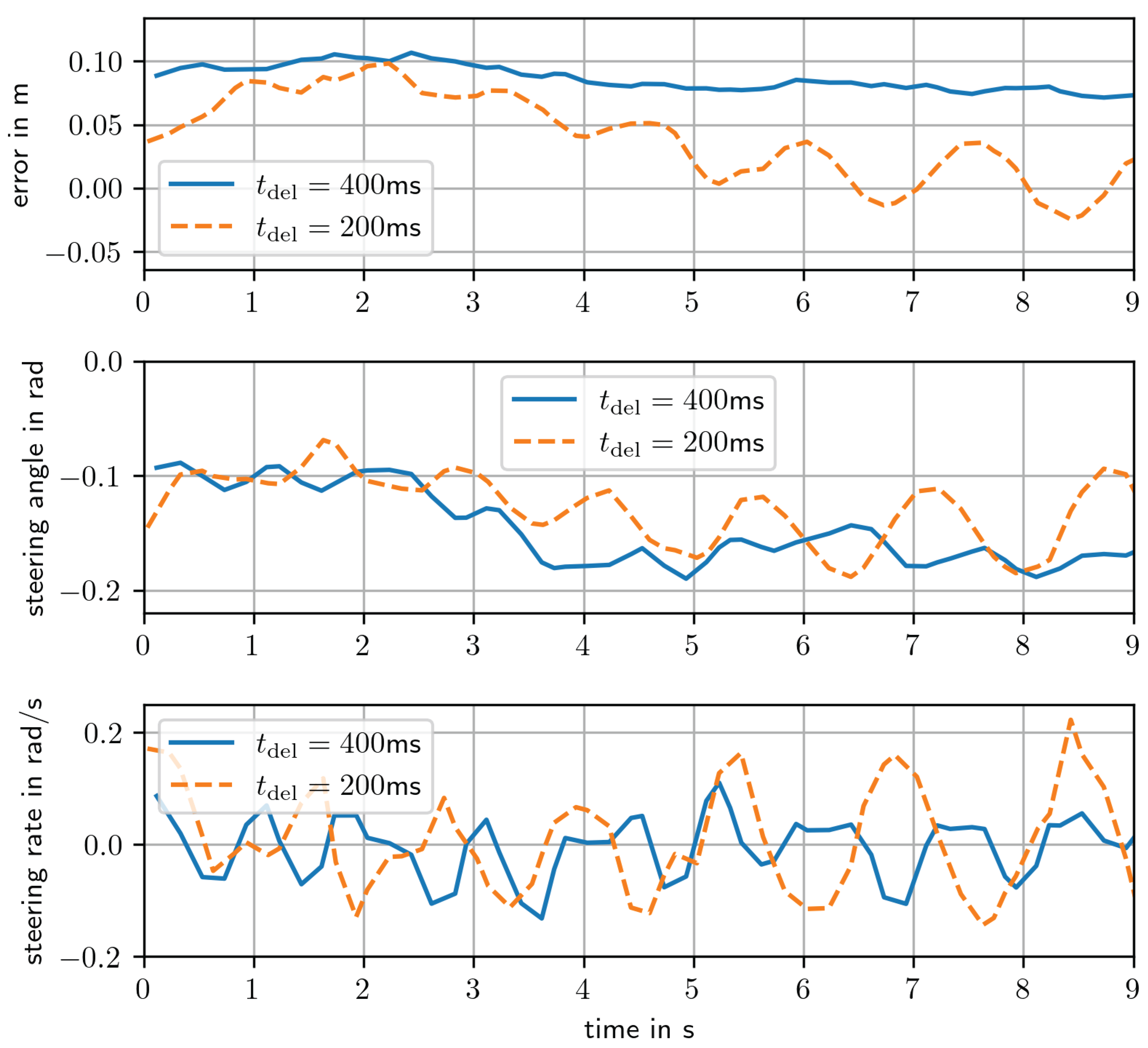
Figure 12.
Single lane-change maneuver with and without look-ahead.
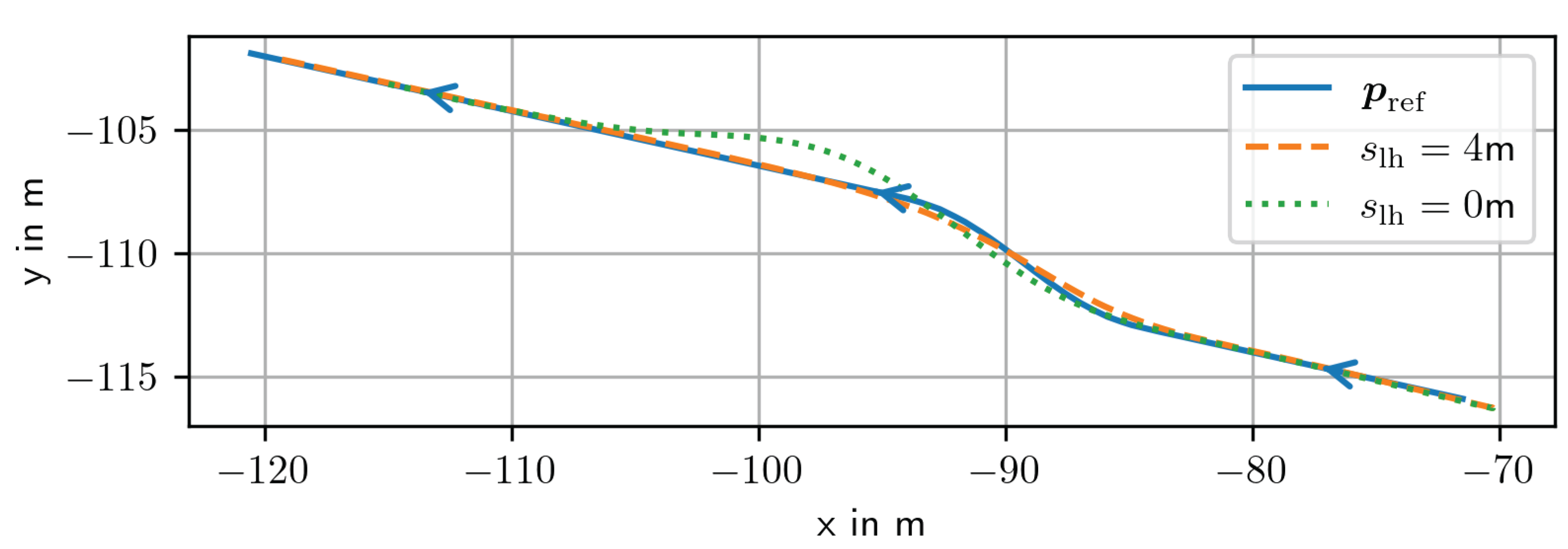
Figure 13.
Lateral error e and steering signal with and without look-ahead.
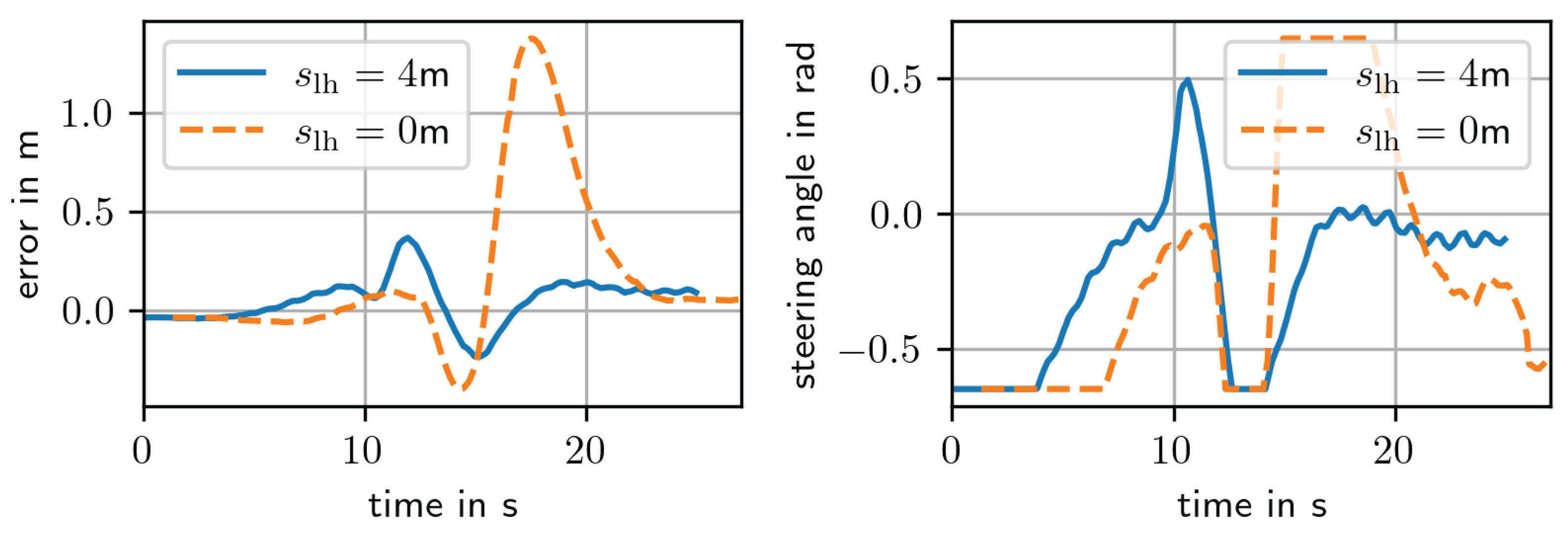
Figure 14.
Results of the double lane-change maneuver, with the controller embedded in an AD system in the real vehicle.
Figure 14.
Results of the double lane-change maneuver, with the controller embedded in an AD system in the real vehicle.
Disclaimer/Publisher’s Note: The statements, opinions and data contained in all publications are solely those of the individual author(s) and contributor(s) and not of MDPI and/or the editor(s). MDPI and/or the editor(s) disclaim responsibility for any injury to people or property resulting from any ideas, methods, instructions or products referred to in the content. |
© 2025 by the authors. Licensee MDPI, Basel, Switzerland. This article is an open access article distributed under the terms and conditions of the Creative Commons Attribution (CC BY) license (http://creativecommons.org/licenses/by/4.0/).
Copyright: This open access article is published under a Creative Commons CC BY 4.0 license, which permit the free download, distribution, and reuse, provided that the author and preprint are cited in any reuse.


