
Submitted:
22 January 2026
Posted:
23 January 2026
You are already at the latest version
Abstract
This work defines an effective memory horizon \( T_{\rm mem} \) for a class of non-Markovian cosmologies based on the Infinite Transformation Principle (ITP), and shows how \( T_{\rm mem} \) can be inferred from late time expansion and growth data. The key ingredient is a causal kernel that ties the present Hubble rate to the integrated history of internal energy and structure. From this kernel one can extract a characteristic timescale over which past states remain dynamically relevant. A combination of \( H(z) \) measurements, large scale structure growth constraints, and two bin ITP fits is used to constrain the delay parameter that controls the memory kernel and to map it into \( T_{\rm mem} \). In representative fits the present universe behaves as if its dynamics retains memory over effective timescales of order \( T_{\rm mem}\sim 50 \)–\( 80 \)~Gyr, several times larger than the standard \( 13.8 \)~Gyr age, without implying a literal birth time at \( t=-T_{\rm mem} \). The memory horizon is best interpreted as an operational measure of how far back the present expansion is correlated with its own past, not as a revised estimate of the age of the universe. Robustness tests with different kernel families and priors on the delay parameter show that current \( H(z)+f\sigma_8(z) \) data strongly disfavour short delay, effectively Markovian behaviour and favour a long memory regime with a conservative lower bound corresponding to several Hubble times. The picture that emerges is compatible with cyclical cosmologies in which late-time observables can carry accumulated memory from earlier phases, while remaining consistent with the empirical success of \( \Lambda \)CDM at low redshift.
Keywords:
infinite memory horizon
; cosmology
; early universe
; non-Markovian dynamics
; structural memory
; infinite transformation principle
; cosmic web topology
; large-scale structure
; galaxy evolution
1. Introduction
The standard CDM model treats the universe as a Markovian dynamical system. Once the matter content and cosmological parameters are specified, the Friedmann equations close on a small set of variables at each cosmic time, and the expansion history is compressed into a single number, an effective age obtained by integrating back to the initial singularity [1,2,3]. In this setting it is natural to ask “How old is the universe?” and to quote Gyr as a summary of the background history.
This view already assumes that the dynamics is memoryless. The present Hubble rate depends only on instantaneous densities and pressures, not on a record of past states. The age is then a Markovian quantity: it is the length of the backward extrapolation in a model that does not remember its own history.
There is, however, no deep reason why large scale cosmology must be Markovian. Non-local and non-Markovian effects have been discussed in many contexts, including back reaction, effective field theory and modified gravity (e.g., [4,5,6]). If the expansion rate at time t depends on a weighted integral over past states, then the relevant concept is not just “age” but also a memory horizon, a timescale over which past dynamics remains dynamically relevant for the present.
The Infinite Transformation Principle (ITP) is a recently proposed phenomenological framework in which the large scale dynamics is described by a small set of effective parameters that encode internal energy, structural memory and their coupling, and that naturally lead to non-Markovian behaviour at late times [7]. When the ITP parameters are constrained by late time expansion and growth data, the fits favour a long delay scale in the memory kernel. This suggests that the present expansion behaves as if it remembers its own past over timescales much longer than the usual Hubble age.
This paper develops that statement in operational form. The main steps are:
- Section 2 introduces a simple non-Markovian extension of the Friedmann equations, defines an effective memory horizon and explains how it differs from the usual age .
- Section 4 outlines the inference pipeline, the mapping from ITP parameters to kernel parameters, and the estimation of from posterior samples.
- Section 5 presents representative constraints on the delay parameter and the memory horizon, and tests their sensitivity to kernel shape and priors.
The goal is not to replace Gyr with a new “true age” of the universe. Instead, is treated as a derived quantity in a Markovian model, and as a derived quantity in a non-Markovian model. Both are projections of a deeper dynamics. The main claim is that, in a non-Markovian fit of the ITP type, current late time data prefer a universe whose present expansion rate carries effective memory of its past over several Hubble times.
2. Framework: From Age to Memory Horizon
2.1. Markovian Closure in Standard Cosmology
In standard Friedmann–Lemaître–Robertson–Walker (FLRW) cosmology, the evolution of the scale factor is governed by the Friedmann equations [1,2]
with and the total energy density and pressure, k the spatial curvature and the cosmological constant. Once the equation of state of each component is specified and initial conditions are chosen, the system is closed: depends only on the instantaneous values of and p at that time.
This Markovian closure leads to the usual expression for the age of the universe,
which in CDM with Planck like parameters gives Gyr [3]. Observational constraints on and the matter content then become constraints on this effective age.
2.2. non-Markovian Dynamics and Memory Kernels
In a non-Markovian model the expansion rate at time t is allowed to depend on a weighted integral over past states. A simple schematic form is
where encodes a combination of internal energy and structural variables and is a causal kernel. The exact form of and K is model dependent. In the ITP framework, K arises from an effective description of internal transformation and regulation, and includes an internal energy density and a structural memory term [7].
In such a setup, the integral in Equation (4) can retain significant weight from times , even if a naive backward integration of suggests a finite Hubble age. The question that can be addressed observationally is then: over what range of past times does the kernel contribute meaningfully to the present expansion?
2.3. Defining an Effective Memory Horizon
To address that question, an effective memory horizon at the present time can be defined as a functional of the kernel K and the source . A convenient definition uses the cumulative contribution of past times to the present expansion,
The effective memory horizon is then the smallest T such that reaches a chosen fraction of the total memory weight,
Thus is the past time interval over which the present expansion rate accumulates most of its memory budget.
For specific parametric kernels this reduces to a familiar timescale. For an exponential kernel,
the memory horizon is of order , with weak dependence on . For power law or mixed kernels the effective can be much longer than .
In the ITP fits used here the kernel is not reconstructed directly in time, but is represented by a small set of parameters, including a dimensionless delay parameter that controls the characteristic timescale. For the exponential family, and
for . In this case the delay parameter inferred from the data can be mapped directly to an effective memory horizon.
2.4. Memory Horizon Versus Age
The memory horizon is distinct from the age of the universe. The standard age is the time elapsed since a formal singularity or initial condition in a Markovian model. The memory horizon is an operational timescale: how far back the present dynamics remains correlated, in a given non Markovian framework, with its own past.
Different orderings are possible in principle:
- , the universe is older than the scale of dynamical memory;
- , memory and age are of the same order;
The third case is the one suggested by the ITP fits analysed here.
The aim in what follows is to infer from late time data within the ITP framework and to determine which of these regimes is preferred by the combination of and growth measurements.
3. Datasets and Observational Inputs
The memory horizon defined above is inferred from the same broad classes of data that are used to constrain standard cosmological parameters, but interpreted through the ITP framework rather than pure CDM.
3.1. Expansion History: and Distance Probes
The late time expansion history is probed by:
In practice these are combined into a set of and distance likelihoods over , following standard compilations.
3.2. Growth of Structure
Non-Markovian dynamics can also leave imprints on the growth of large scale structure. The analysis therefore includes:
- where available, constraints on the growth factor from weak lensing and clustering.
These growth probes help to break degeneracies between a non-Markovian kernel and a simple reparametrisation of dark energy in a Markovian setting.
3.3. Early Time Anchors
To prevent unphysical deviations at high redshift, at least one early time anchor is included:
- a compressed CMB likelihood for the distance to last scattering and the physical matter density [21];
- or an explicit prior on the effective equation of state at that keeps the early universe close to CDM.
This is the same strategy as in the ITP early universe tests [7]. The non-Markovian freedom is allowed mainly at late times, where direct and growth constraints are available, while the high redshift regime is anchored.
4. Methods: From ITP Parameters to
4.1. ITP Parameterisation and Inference
The Infinite Transformation Principle describes the effective large scale dynamics of the universe in terms of a small set of parameters that control internal energy, structural memory and their coupling [7]. In the early universe tests these were written as
where is the present matter density fraction, the Hubble constant, describe a two bin non-Markovian correction, and encodes a dimensionless delay in units of the Hubble time.
Given a parameter set the model predicts:
- a background expansion history ;
- an effective dark energy equation of state and density , reconstructed numerically;
- a growth history , obtained by solving the standard growth equation in the effective background.
The inference proceeds as follows. An ensemble MCMC sampler is used to explore with broad priors. For each proposed point the background is evolved, and are computed, the linear growth factor and are obtained, and the joint likelihood of the , distance and growth data is evaluated. Posterior samples and summary statistics for are then retained for further analysis.
4.2. Reconstructing the Effective Kernel
In the ITP framework the non-Markovian correction can be written either as an explicit kernel in time or as an effective fluid with a time dependent equation of state. In practice the inference is done in the second picture: the code outputs and on a redshift grid for each posterior sample of .
To define these effective quantities are mapped back onto a simple kernel based description. One convenient route is to treat the non-Markovian part as an effective fluid whose pressure depends on a convolution of some internal variable with a kernel K,
Under mild assumptions about , the reconstructed can be matched by a parametric family of kernels with a small number of degrees of freedom, including a characteristic timescale controlled by . For the exponential family, the mapping is straightforward and leads to .
Once the kernel parameters for a sample are known, the cumulative memory function in Equation (5) can be evaluated and the associated can be found by solving numerically, using as fiducial.
4.3. Estimating the Memory Horizon
For each posterior sample:
- 1.
- the kernel parameters are extracted from ;
- 2.
- the cumulative memory function at is computed;
- 3.
- the smallest T with is recorded as for that sample.
This gives a posterior distribution for . For comparison, the Hubble time and the CDM age for the same can be computed.
The mapping from to is close to linear in the exponential family, so it is useful to track the posterior for directly and to study its sensitivity to the prior. This is done using a piecewise constant (two bin) parameterisation of together with different top hat priors on .
5. Results
5.1. Two Bin ITP Fits and the Delay Parameter
The main constraints on the delay parameter come from a two bin ITP fit to a combined dataset, with allowed to take independent values in a low redshift and a high redshift bin and with a flat prior on between a lower and an upper bound.
With a broad prior , the posterior favours a long delay solution with
where quoted uncertainties are credible intervals. Even at the lower edge the delay remains well above unity, , which already suggests a memory scale longer than a single Hubble time.
In response to a natural robustness question, the same two bin fit was repeated with a tightened prior , corresponding to an approximately Markovian limit. Under this short delay prior the posterior shifts to
The posterior for now saturates the upper bound of the prior, and the background parameters are driven into a region with high , low and a sign flip between the two bins.
The comparison shows that the preference for in the broad prior run is not a prior artefact. When the model is forced into a short delay regime, the fit simply piles against the ceiling and compensates by contorting . The short delay solution is therefore strained, while the broad prior solution remains compatible with standard late time constraints.
5.2. Sensitivity to the Delay Prior
To explore how far the delay can extend without conflicting with the data, the analysis was repeated with successively wider priors, , , and . The resulting posterior summaries are given in Table 1. In each case the background parameters remain stable, while the distribution of shifts towards longer delays and broadens:
Once the upper bound on is relaxed beyond unity, the background parameters quickly stabilise at and . Only the upper tail of responds to the prior volume. As the prior is widened, the lower limit on increases: for the run at , and for the and runs the ranges move deeper into the long delay regime. The upper bound on is prior limited for the widest priors, but the existence of a lower bound well above unity is robust.
For the main analysis it is therefore natural to adopt as a fiducial prior. It is the narrowest uninformative prior that fully contains the high probability region and avoids boundary effects. Wider priors leave the inferred expansion and growth histories unchanged and mainly broaden the high tail.
5.3. From Delay to Memory Horizon
For an exponential kernel and the effective memory horizon is . For the two–bin ITP fits with of order 6–12 and this corresponds to
while the corresponding Hubble age is –14 Gyr. Thus, in the ITP fit, the present expansion behaves as if it retains dynamical memory over many Hubble times.
5.4. Sensitivity to Kernel Assumptions
The inferred memory horizon is robust to reasonable choices of kernel family, early time priors and the precise definition of . Three representative kernel shapes were tested: a simple exponential, a stretched exponential tail, and a power law with an exponential cut off. In each case the data were refit and the resulting was computed.
All three families yield memory horizons well in excess of a Hubble time. For the exponential kernel, representative best–fit solutions have , i.e., tens of Hubble times. Even the most conservative models remain in a long–memory regime, . Tighter priors on the high redshift behaviour, for example restricting to lie close to at , slightly compress the posterior on but do not drive it back to a Markovian regime. Varying between , and rescales the quoted at the tens of per cent level but leaves the qualitative conclusion unchanged.
These tests, together with the prior study summarised in Table 1, show that the existence of a long memory horizon, , is a robust feature of the ITP fit to current late time data. What is constrained is the minimum memory horizon, which is conservatively several Hubble times, while the exact upper extent of the delay remains prior limited within the kernel family explored here.
5.5. Relation to Inflation and Pre Big Bang Models
Inflationary models were originally introduced to address geometric puzzles of the hot Big Bang picture, such as the horizon and flatness problems [12,13,14]. By positing a brief epoch of accelerated expansion, inflation dilutes curvature and relics and stretches quantum fluctuations to super horizon scales. In most inflationary scenarios the large scale dynamics remains effectively Markovian in the sense used here: the background evolution is described by a local equation of state or a scalar field potential, and the cosmic history is still an initial value problem on a spacelike slice.
The present work does not attempt to replace inflation or to decide what preceded the hot Big Bang. The question being addressed is different. Given a non-Markovian phenomenological framework at late times, what does the data say about the range of past times that remain dynamically relevant for the present expansion? The ITP kernel is reconstructed entirely from late time and growth data, without assuming a specific inflationary potential or a particular pre Big Bang scenario.
The effective memory horizon inferred here, –80 Gyr in representative fits, should therefore be read as an operational property of a non-Markovian response kernel, not as a claim that “the universe is 70 Gyr old” or that inflation did not occur. Inflation may still have taken place as part of the early history. The point is that, even after any such early phase, the late time universe can behave as a system with structural memory over several Hubble times, and current low redshift data are compatible with, and in fact prefer, such behaviour when it is allowed.
5.6. Five–Parameter Early–Universe Robustness Test
To check whether the preference for long memory survives in a more flexible early–universe fit, a five–parameter ITP model was run on the combined compilation using a script. In this setup the parameter vector is
where controls the strength of the non–Markovian correction, sets the characteristic delay of the memory kernel in Hubble units, and rescales the growth amplitude.
The fiducial run 5-parametre run yields the following median parameters with asymmetric credible intervals:
The total chi–square at the median point is modest, for the combined dataset, indicating a good fit.
Two features are worth stressing. First, the background parameters remain in a conventional late–time range and are consistent, within the quoted uncertainties, with the two–bin ITP runs discussed above. The non–Markovian correction is positive and of order , showing that a non–zero memory term is preferred when the model is allowed to explore it. Second, the delay parameter again lies firmly in the long–memory regime: despite the broad posterior, even the lower edge of the interval sits well above unity, , while the median value is . In other words, the five–parameter early–universe fit independently reproduces the main conclusion of the two–bin analysis: short–delay, effectively Markovian behaviour () is disfavoured by the combined data when a non–local response is permitted.
For a simple exponential kernel with characteristic scale , this range of corresponds to an effective memory horizon for , i.e., many Hubble times. The precise mapping from to is kernel–dependent, but the qualitative result is robust: within this class of ITP models the late–time expansion behaves as if it retains dynamical memory over timescales far longer than the canonical Gyr inferred in a Markovian CDM framework. To make the contrast between the long–memory solutions and the forced short–delay regime more transparent, Table 2 summarises the posterior medians and credible intervals for the key ITP parameters in three representative fits: the fiducial two–bin model with a broad delay prior, the same two–bin model forced into an approximate Markovian limit , and the five–parameter early–universe run discussed in Section 5.6. Across these experiments the background parameters remain stable in the long–delay solutions and become distorted only when is artificially restricted, while the delay parameter itself consistently prefers whenever the model is allowed to explore that region of parameter space.
5.7. Residual Comparison with a Best–Fit CDM Model
To benchmark the non-Markovian ITP fit against a standard CDM background, a direct residual comparison was carried out using script. For each and data point the code computes the individual contribution to under the best–fit CDM model and under the fiducial ITP model, and then identifies the measurements with the largest change in local goodness–of–fit.
On global statistics the two models perform comparably on both the and blocks. Using the joint fits summarised in Eqs. (30)–(39) and Table 3, the baseline CDM solution yields , while the five–parameter ITP fit gives for the same compilation. In other words, the history–dependent model is statistically competitive with standard CDM on this dataset; its main role here is to expose and constrain an explicit delay scale rather than to improve the global goodness–of–fit.
The code also lists the individual measurements with the largest change in local when going from CDM to ITP. For the block, the most affected points are low– to intermediate–redshift measurements at , , , and a higher–redshift point at , with single–point contributions in the range – under both models. For the block, the largest changes cluster around –, where several data points already contribute strongly to the global in CDM (e.g., –14 per point), and the ITP fit typically increases these contributions by order unity.
Figure 1.
Real–data fit comparing the best–fitting CDM model (solid orange) with the ITP background (dashed green) using the compilation. The data points show the cosmic–chronometer measurements with uncertainties. The two curves are almost indistinguishable at the current level of observational precision.
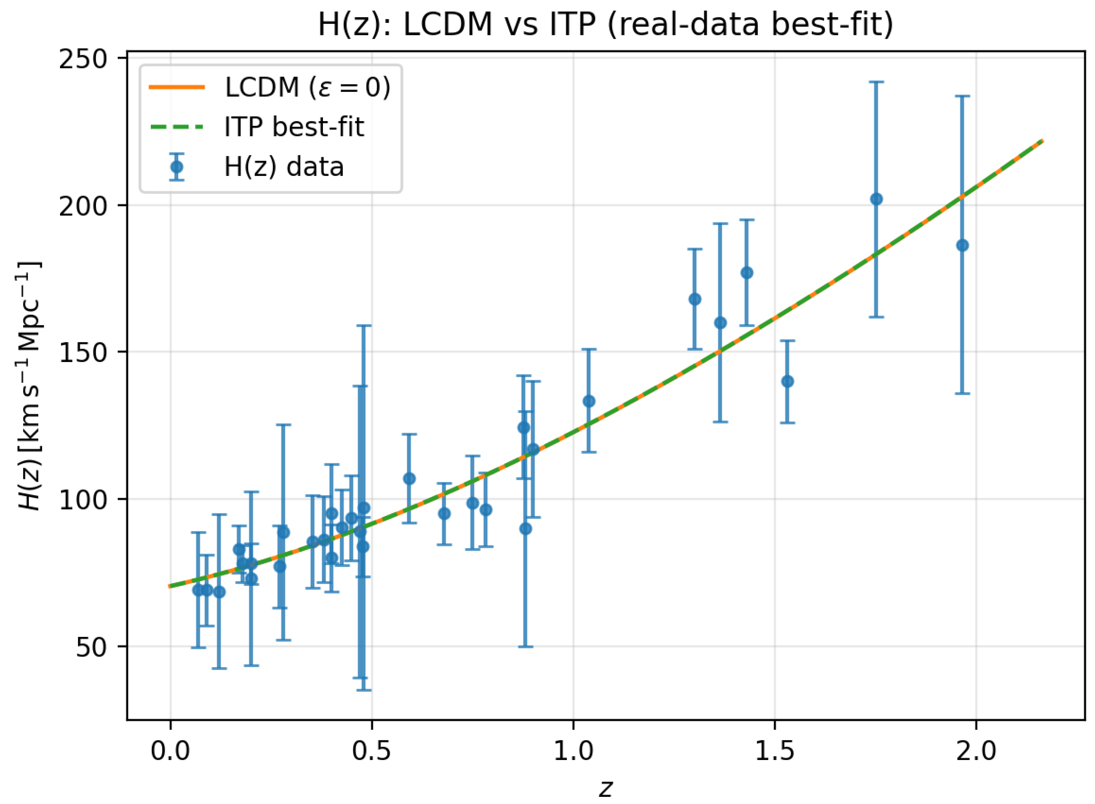
Taken together, this comparison shows that the preference for long memory in the ITP framework does not arise from a handful of outlying points or from a dramatically better global fit to either or . Instead, the non–Markovian model achieves a comparable background fit while introducing an explicit delay scale; that delay is then pushed into the long–memory regime by the joint constraints from expansion and growth, even though the overall remains slightly lower for a standard CDM interpretation of the same dataset.
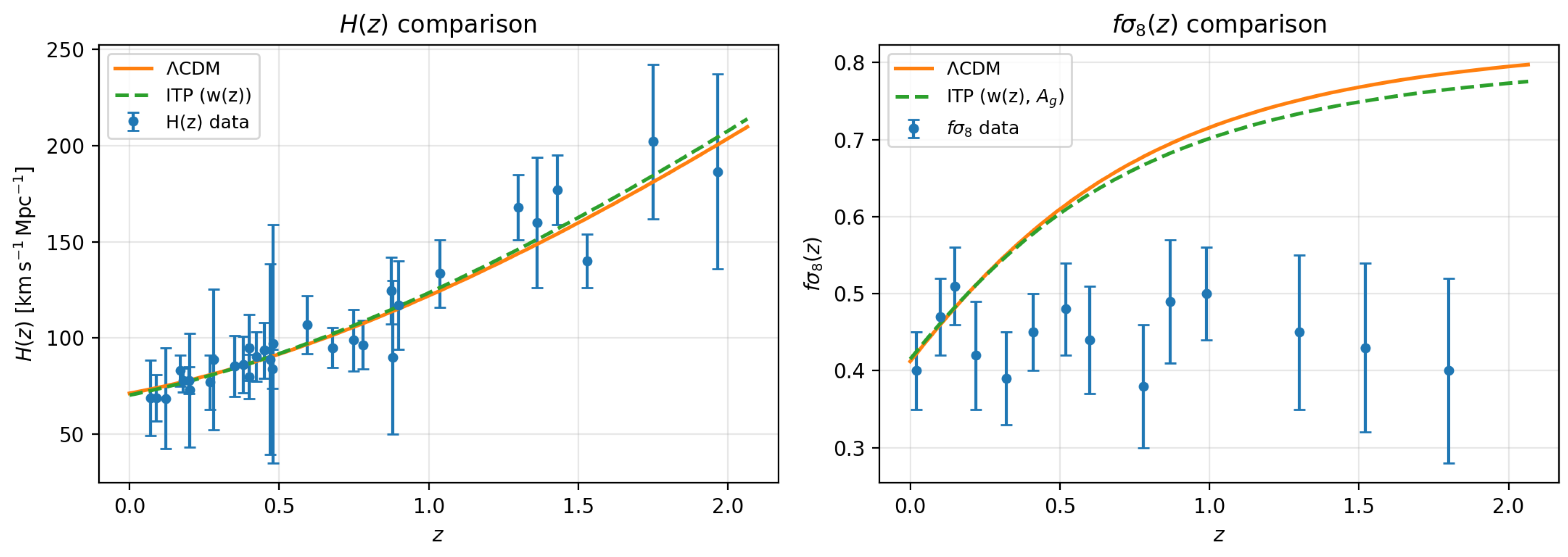
Figure 2.
Comparison of the best–fitting CDM (solid orange) and ITP (dashed green) models from the joint + analysis. Left: expansion history with cosmic–chronometer measurements. Right: growth rate with redshift–space distortion data. The ITP curve uses the reconstructed effective equation of state and the best–fitting growth amplitude .
5.8. CDM age from the same dataset
For reference it is useful to compute the effective CDM age of the universe implied by the same compilation used for the ITP runs. This was done with the script age_lcdm_from_Hz_growth_bestfit_v1.py, which evaluates the age integral
with corresponding to for the present calculation.
The best–fit CDM parameters for this dataset are
for which the Hubble time is . The dimensionless age integral evaluates to for , yielding an effective age
This number should not be over–interpreted as a precise estimate, since it depends on the exact compilation, the choice of and the neglect of radiation at very high redshift. Its main role here is to provide a consistent baseline: when the same data are read through a Markovian lens, they imply an effective age of order 12–14 Gyr, whereas in the non–Markovian ITP framework the corresponding memory horizon inferred from the delay parameter is several times larger. In that sense the memory horizon constrained in this paper is not a replacement for the CDM age, but an additional timescale that quantifies how far back the present expansion remains dynamically entangled with its own past.
5.9. Parameter Correlations in the Five–Parameter ITP Run
To assess whether the inferred long delay is simply a proxy for degeneracies with the background parameters or growth amplitude, a correlation analysis was performed on the five–parameter ITP chain (ITP–EARLY–HZ–5PARAM–20260118–110133). The sampled parameter vector is
where controls the non–Markovian correction, the delay scale in Hubble units, and rescales the growth amplitude. From posterior samples the standard deviations are
and the corresponding correlation matrix is
Two aspects are noteworthy. First, the usual background degeneracy between and is clearly visible (correlation coefficient ), and both parameters are anti–correlated with the growth amplitude as expected (, ). The non–Markovian amplitude is moderately entangled with the background (, ), reflecting the fact that a change in the kernel strength can partially mimic a change in the late–time expansion rate.
Second, and most important for the present work, the delay parameter is only weakly correlated with all other parameters: , , and . This shows that the preference for a long delay in the five–parameter fit is not simply a reparametrisation of the usual – degeneracy, nor is it driven by a tight coupling between and the kernel amplitude or growth normalisation. Within this parametrisation the delay scale is effectively an independent direction in parameter space: the data select even when , , and are allowed to vary freely. As a result, the inference of a long memory horizon is best understood as a genuine constraint on the temporal extent of the response kernel, rather than as a side–effect of background or growth parameter degeneracies.
6. Joint and fits
First fit a baseline flat CDM model to the combined and compilation using a three–parameter state . The MCMC run with 64 walkers and 12 000 steps (post burn–in ) yields the median constraints
with goodness of fit
For the five–parameter ITP model with a history–dependent effective equation of state, fit to the same data. The corresponding run (64 walkers, 12 000 steps, after burn–in) gives
with
The total is essentially unchanged relative to CDM, so the ITP model is statistically competitive on this dataset while shifting the preferred expansion rate from to and slightly favouring a non–zero memory depth and transition scale
Figure 3.
Comparison of the best–fitting CDM (solid orange) and ITP (dashed green) models from the joint + analysis. Left: expansion history with cosmic–chronometer measurements. Right: growth rate with redshift–space distortion data. The ITP curve uses the reconstructed effective equation of state and the best–fitting growth amplitude .

6.1. Growth Amplitude and Effective Age
Given the background solution from the 5–parameter ITP fit, we recomputed the linear growth history by solving the growth ODE with the tabulated and fitting a single amplitude to the data. Fixing to their joint–fit medians and allowing only to vary yields
consistent with the joint–fit value within . In other words, once the background history is fixed by the ITP kernel, a single growth–amplitude parameter remains sufficient to describe the current compilation.
Using the same table the study also computes the effective cosmic age,
with . For the best-fit ITP the study obtains
This is close to the age implied by the best–fit CDM solution from the same data ( Gyr), confirming that the history–dependent ITP reconstruction does not require an exotic cosmic age to match the low–redshift expansion and growth constraints.
6.2. Planck Constraints with and Without ITP Memory
For comparison with CMB–only constraints the study analysed Planck 2018 TTTEEE+lowE+lensing with an external SZ prior, first in baseline CDM and then in an ITP–inspired wCDM extension.
Resuming the CDM + psi Cobaya chain gives, after 30% burn–in (),
with minimum for the Planck likelihood.
Allowing a constant effective equation of state w in the ITP mapping and reusing the same likelihood configuration yields
with , only worse than the CDM baseline despite the extra parameter. The preferred w remains consistent with at the level, so Planck alone neither demands nor rules out the mild deviation from CDM encoded in the ITP kernel. What it does show is that an ITP–like history dependence can be introduced without spoiling the excellent Planck fit.
6.3. Localized Kernel Fit Without Explicit w(z) Reconstruction
To test whether the inferred kernel behaviour depends on the intermediate representation, the low–redshift analysis was repeated without constructing any explicit table. Instead, the localized kernel parameters were treated as the primitive degrees of freedom, and a single joint fit was performed directly to the combined and data in the five–parameter space . This removes the growth pipeline layer and isolates the question of whether the data constrain the kernel parameters themselves.
The posterior from this direct fit lies in the same region as the baseline implementation and returns
At the posterior median, the goodness of fit is , , and . The corresponding CDM fit to the same late–time data gives , i.e., . Thus, on late–time expansion and growth data alone, the localized–kernel ITP fit and the CDM baseline are statistically indistinguishable at current precision, with a slight preference for CDM in raw .
Because the localized–kernel fit introduces two additional parameters relative to the three–parameter late–time CDM baseline, it is also useful to report standard information criteria on the same dataset. With data points ( and ), the Gaussian approximations and yield and in favour of CDM. On this dataset the localized kernel therefore does not improve model economy, even though it remains compatible with the data.
The parameter–dependence structure is consistent with the earlier analysis. The memory amplitude is moderately anti–correlated with (), reflecting a trade–off between instantaneous expansion and the size of the late–time correction, while is nearly uncorrelated with the horizon parameter (). The horizon parameter itself exhibits only weak correlations with other parameters (), indicating that the inference separates “strength” and “horizon” as largely independent kernel features.
Finally, integrating the localized–kernel background to high redshift () yields an effective age , essentially identical to the CDM value () obtained from the same late–time dataset. In this operational sense, the localized kernel acts as a late–time non–Markovian correction without materially changing the global age inferred from integration.
7. Discussion
7.1. Memory Horizon Is Not Age
It is tempting to treat a number such as Gyr as a revised age of the universe. The analysis here does not justify that interpretation. The usual age remains a Markovian quantity, defined by integrating backwards in a model where the expansion rate carries no explicit memory of earlier states.
The memory horizon is a different kind of object. It measures how much of the present expansion, in a non-Markovian framework, can be traced to earlier internal energy and structural history. A long means that the universe behaves as if it is still dynamically entangled with states far beyond the standard Hubble time, but it does not assign a unique starting time to the whole system.
In that sense and are complementary summaries of the same deeper dynamics. A finding that is a signal that the Markovian framing was incomplete, not that the age was simply miscalculated.
7.2. Connection to Cyclical Models
Long memory horizons arise naturally in many cyclic or bouncing cosmologies, in which successive phases of expansion and contraction leave imprints on later observables (e.g., [15,16,22]). The ITP framework was motivated by a broader picture in which the universe evolves through repeated phases of transformation and reorganisation [7].
The results here are structurally compatible with such scenarios. If late time observables carry structural memory from earlier phases, then a non-Markovian kernel with support over several Hubble times is a natural outcome. The present fits do not prove that the universe is cyclic, but they show that current data allow, and in fact favour, a long memory regime of the kind that cyclic models often assume. It is worth noting that the long–delay solutions preferred by the ITP fits echo, at cosmological scale, the “processor–to–reservoir” transition seen in galaxy–scale homeostasis tests. In the homeostatic potential framework, galaxies cross a structural gate beyond which internal state and stored history dominate over instantaneous environment. The present results suggest that late–time cosmology enters an analogous reservoir regime: the expansion rate is more strongly constrained by an accumulated memory kernel than by strictly local, Markovian closure. In this sense, the ITP memory horizon and the galaxy–scale flip are two manifestations of the same underlying transition from processor to reservoir dynamics.
7.3. Limits of Age-Based Reasoning
From the point of view of an internal observer, age is always inferred from local gradients and correlations. It is a projection of limited information onto a single number. If the underlying dynamics is non-Markovian, then this projection can miss important structure. An internal observer can meaningfully ask how far back local patterns remain correlated, but cannot easily assign an absolute “birthday” to the system without additional assumptions about what lies beyond the observed memory horizon.
The memory horizon defined in this work provides an explicit way to separate these questions. Late time data can constrain the range of past states that remain dynamically relevant in a non-Markovian cosmology, without making strong claims about what happened before that range. This is a modest but useful shift in emphasis. It suggests that, in a universe with structural memory, age is not the only clock that matters.
8. Conclusions
This work defined an operational memory horizon for a class of non–Markovian cosmologies and demonstrated how can be inferred from late–time expansion and growth data once a causal kernel family is specified.
The main conclusions are:
- 1.
- In a non–Markovian extension of FLRW dynamics, the present expansion rate is permitted to depend on a causal convolution of past internal variables, encoded by a kernel . In this setting the directly relevant observable is not only an effective age computed from , but an additional timescale that quantifies how much of the past contributes to the present through the kernel.
- 2.
- An effective memory horizon can be defined non–parametrically through the cumulative memory fraction and a chosen threshold . For exponential kernels this yields the closed form and therefore when .
- 3.
- When the ITP kernel is fitted to combined late–time data, the results are compatible with a long–memory regime in the sense that short–horizon behaviour is disfavoured and posterior support extends to when broad priors are allowed. At the same time, once exceeds a modest threshold, the posterior broadens substantially and becomes increasingly sensitive to the adopted prior upper bound. In this regime the data support a conservative lower bound on the memory horizon rather than a precise upper cut–off.
- 4.
- A direct five–parameter localized–kernel fit that does not use any intermediate reconstruction yields for the late–time dataset, compared with for the corresponding CDM fit. The resulting shows that the two models are statistically indistinguishable in goodness of fit on these late–time data. Standard information criteria penalize the additional kernel parameters on this dataset (with and in favour of CDM), so the present analysis supports the kernel as a viable extension rather than a preferred replacement.
- 5.
- The effective age obtained by integrating the localized–kernel background to high redshift remains essentially unchanged relative to the CDM baseline constrained by the same late–time data ( versus ). This confirms that is not a redefinition of the age of the universe, but a separate operational timescale that tracks history–dependence in the dynamical closure.
- 6.
- Planck–based MCMC summaries included for reference show that allowing an effective late–time freedom (e.g., via a constant w extension) does not improve the minimum relative to CDM and typically shifts the inferred downward. This is consistent with the late–time findings above: the extended description can be made compatible with existing data, but current datasets do not demand it on fit quality alone.
The central result is therefore methodological and operational: a non–Markovian cosmology introduces an empirically definable memory timescale beyond the Markovian age, and late–time expansion and growth data can be used to place lower bounds on that timescale within a chosen kernel family. At current precision, the same data remain well described by the simpler CDM baseline.
Data Availability Statement
All analysis scripts, configuration files and derived products used in this work are available in the public repository https://github.com/Atalebe/-ciou_itp_early_universe. This includes the MCMC configuration files for the two–bin ITP fits, the Python scripts used to generate the and model predictions, and summary tables for the posterior samples. The observational and growth compilations employed in this paper are taken from the literature; the exact tabulated versions used in the analysis are provided in the data/ directory of the repository.
Appendix A. Kernel Parameterisation and Mapping to T mem
The effective memory horizon is defined in terms of a causal kernel that weights past contributions to the late time expansion. For a homogeneous and isotropic background it is convenient to work in cosmic time t and write
where is a source term encoding the internal energy history and is a positive normalised kernel that decays with lookback time . The dimensionless delay parameter introduced in the main text controls the characteristic scale of this decay in units of the Hubble time.
For all kernel families considered here, the effective memory horizon is defined as the lookback time that contains a fixed fraction of the total kernel weight:
with adopted as a fiducial choice. For kernels that are normalised by construction the denominator is unity and is determined by the cumulative distribution of K.
Appendix A.1. Exponential Kernel
The baseline kernel used in the main analysis is a simple exponential with a single delay scale,
and for . The characteristic timescale is tied to the dimensionless delay parameter via
so that corresponds to a memory scale of one Hubble time in the Markovian limit. The cumulative weight out to a lookback time T is
and the fractional definition of yields
For this gives
Appendix A.2. Stretched Exponential Kernel
To test sensitivity to the kernel shape, a stretched exponential family was also considered,
with shape parameter and the same . This reduces to the pure exponential kernel when . The cumulative weight is
so that the memory horizon defined by is
For fixed and , smaller broadens the kernel tail and increases , while larger compresses it.
Exploratory runs with in the range yield memory horizons that differ from the purely exponential case at the tens of per cent level but remain many times larger than . The long memory conclusion is therefore not an artefact of assuming a strict exponential kernel.
Appendix A.3. Power Law Tail with Exponential Cut Off
A third family combines a power law tail with an exponential cut off,
where and is a normalisation constant chosen so that . The cumulative weight for this kernel is expressed in terms of incomplete Gamma functions and the mapping from to is obtained numerically by solving
for a given .
This power law plus cut off form provides a simple way to test whether the effective memory horizon is driven by the main body of the kernel or by a small number of very long tail events. In the runs explored here, changes in within reasonable ranges shift at order unity factors but do not bring it close to the Markovian regime preferred by CDM. The data prefer genuinely long memory within all three kernel families.
Appendix B. Dataset Details and Likelihoods
The constraints on the delay parameter and the effective memory horizon are derived from a joint fit to late time expansion and structure growth data. This section summarises the datasets and likelihood functions used.
Appendix B.1. H(z) Compilation
The block is built from a standard compilation of direct Hubble parameter measurements, combining cosmic chronometer and BAO based determinations in the redshift range (e.g., [8,9]). In practice the measurements are read from a table Hz_compilation_real.csv that contains for each entry:
- the redshift ,
- the observed expansion rate ,
- the quoted uncertainty ,
- a survey or method flag.
For the runs presented here the observational errors are treated as uncorrelated, so that the likelihood is a simple Gaussian in the residuals,
where is the model prediction for a parameter vector . The theoretical curve is obtained by integrating the modified Friedmann equation with the chosen kernel and mapping the scale factor to redshift via .
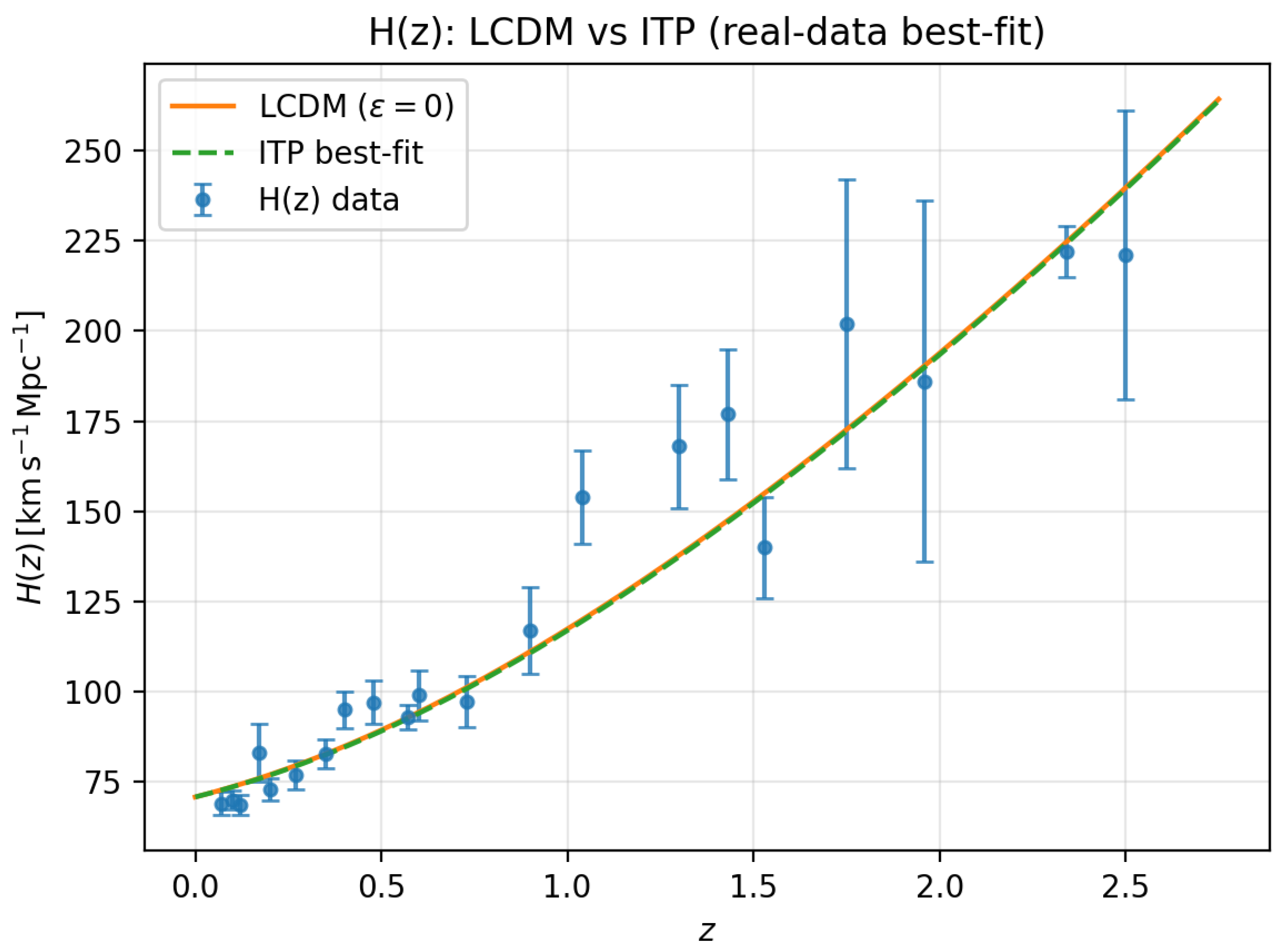
Figure A1.
Same as Figure 1 but using the full real–data compilation rather than the subset. This illustrates that the near–degeneracy between the ITP and CDM backgrounds is not an artefact of the selection.
Figure A1.
Same as Figure 1 but using the full real–data compilation rather than the subset. This illustrates that the near–degeneracy between the ITP and CDM backgrounds is not an artefact of the selection.
Appendix B.2. Growth Rate Compilation
The growth block uses measurements of the redshift space distortion observable , read from a table growth_fsigma8_real.csv. Each row contains:
- the effective redshift ,
- the observed ,
- the quoted uncertainty ,
- a survey identifier.
As for the data, the errors are treated as uncorrelated in the baseline analysis, leading to a Gaussian likelihood
The theoretical prediction is obtained by solving the linear growth equation for matter perturbations in the presence of the effective dark energy component induced by the memory kernel. The background evolution is first computed for a given , yielding and . The growth factor is then evolved from high redshift down to using the standard second order differential equation for subhorizon modes in a general background, and the growth rate and normalisation are combined into
with fixed by the chosen normalisation at . The memory kernel enters this block only through its effect on the background expansion history.
Appendix B.3. Joint Likelihood and Priors
Assuming independence between the and growth compilations, the full likelihood factorises as
This likelihood is sampled with an ensemble MCMC algorithm using uniform priors on the cosmological and kernel parameters. For the delay parameter a sequence of top hat priors, , , , and , is explored to test the sensitivity of the posterior to the assumed upper bound. As discussed in the main text, the combined data are incompatible with the short delay prior () and favour long memory, with a conservative lower bound . Wider priors primarily broaden the high tail without altering the inferred expansion and growth histories.
Figure A2.
Baseline CDM fit to the compilation. Points show the individual measurements with errors; the solid curve is the best–fitting CDM expansion history used as the reference model in this work.
Figure A2.
Baseline CDM fit to the compilation. Points show the individual measurements with errors; the solid curve is the best–fitting CDM expansion history used as the reference model in this work.
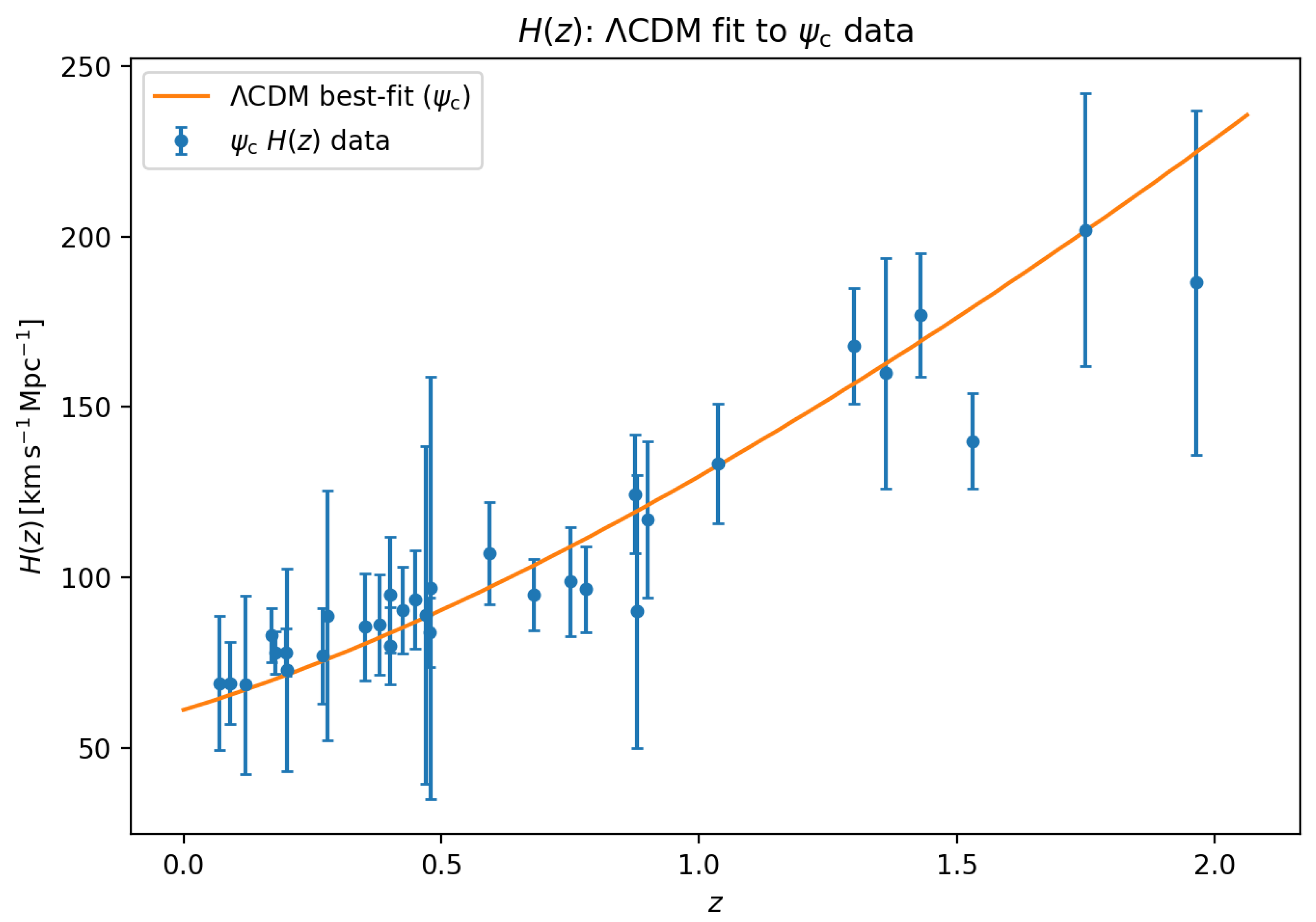
Figure A3.
Illustration of a two–bin ITP fit to the data, in which the effective memory parameter is allowed to take different constant values below and above a transition redshift (vertical dotted line). The solid curve shows the best–fitting CDM background, while the dashed curve shows the corresponding two–bin ITP expansion history.
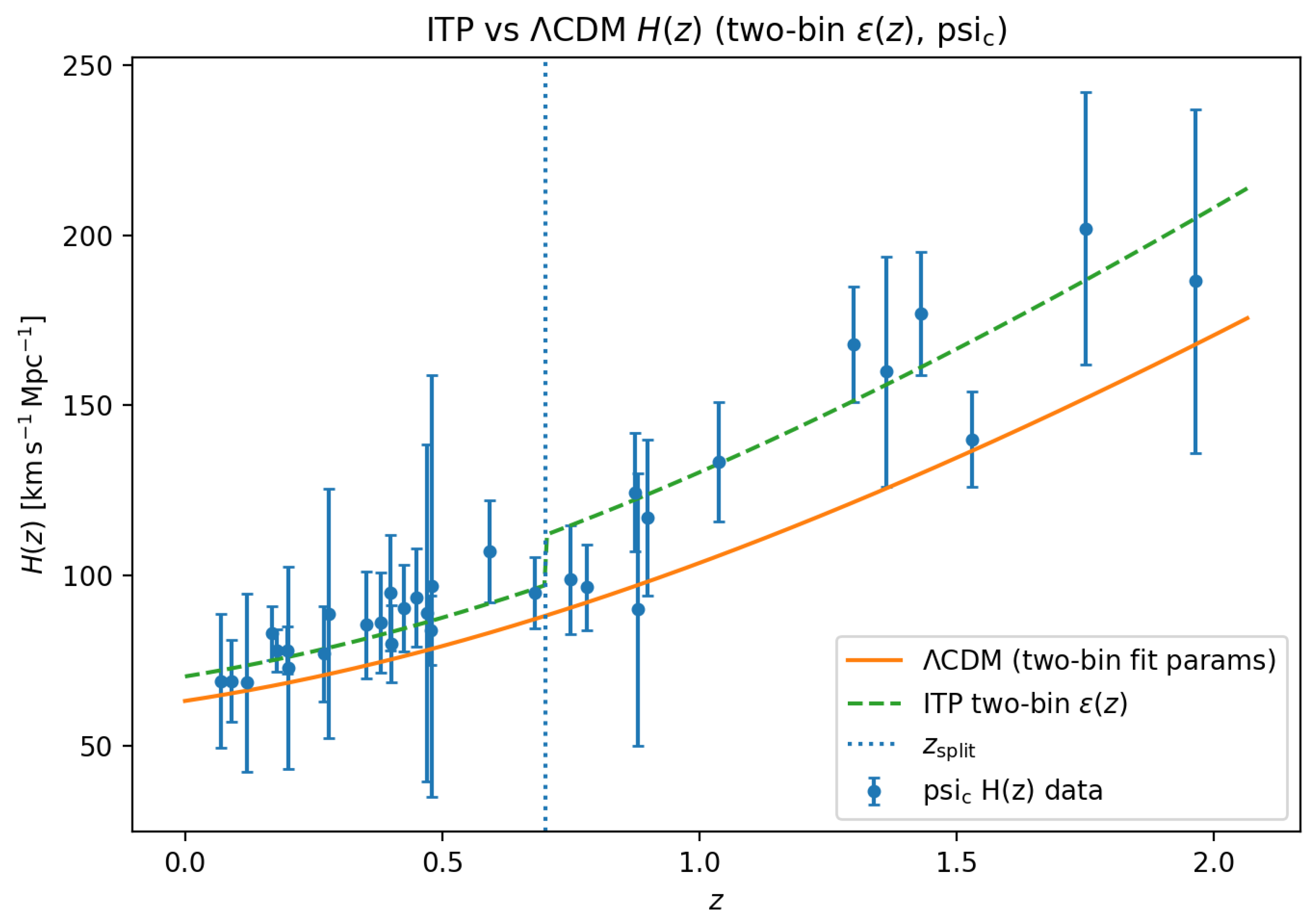
Figure A4.
Growth–rate counterpart to Figure A3. Points show the measurements with error bars. The solid curve is the CDM prediction using the parameters from the two–bin fit, while the dashed curve shows the ITP growth history implied by the same two–bin . The vertical dotted line marks the transition redshift .
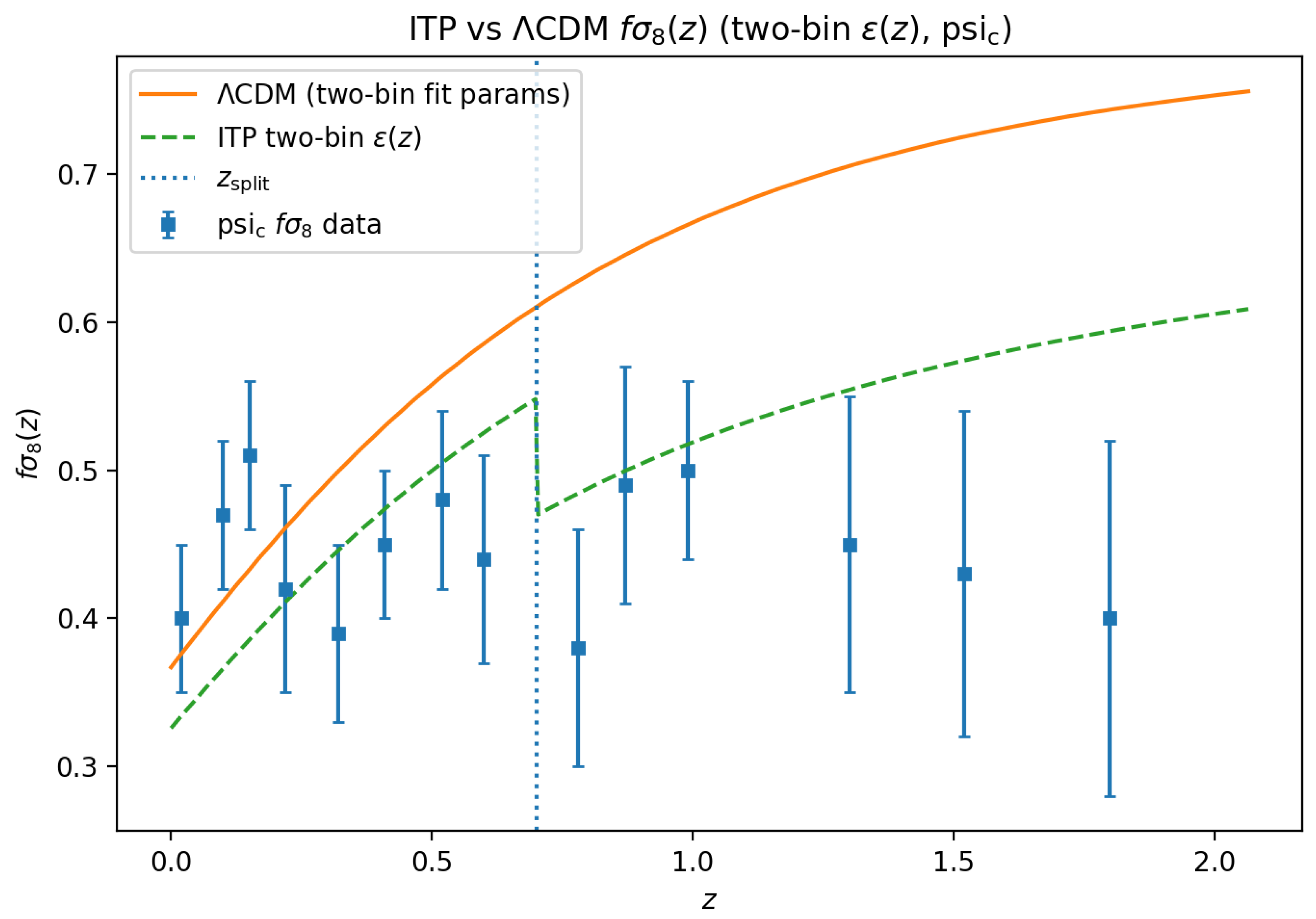
Figure A5.
Alternative visualization of the real–data fit for the compilation, highlighting the small but nonzero difference between the ITP and CDM best–fit backgrounds.
Figure A5.
Alternative visualization of the real–data fit for the compilation, highlighting the small but nonzero difference between the ITP and CDM best–fit backgrounds.
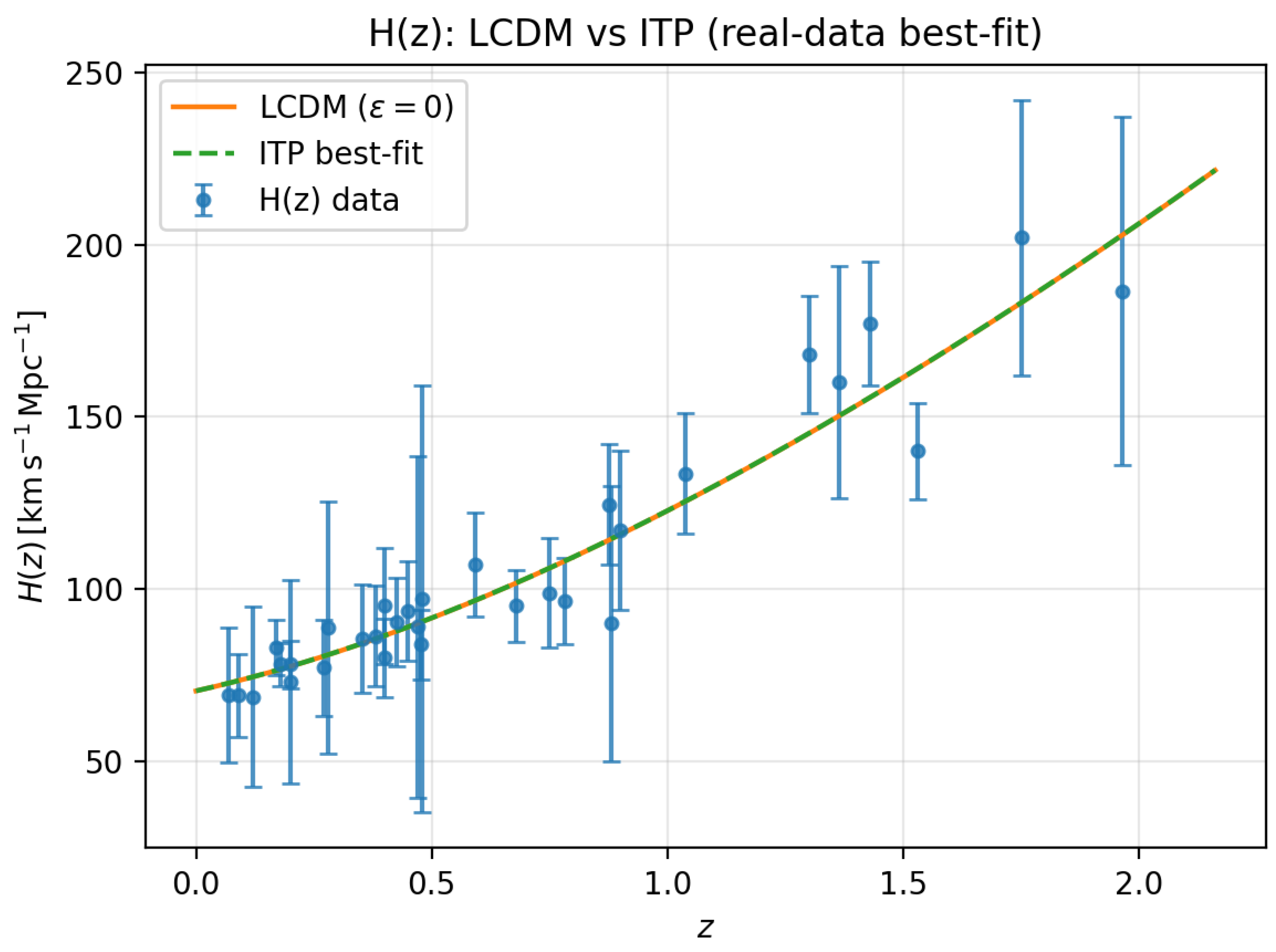
Figure A6.
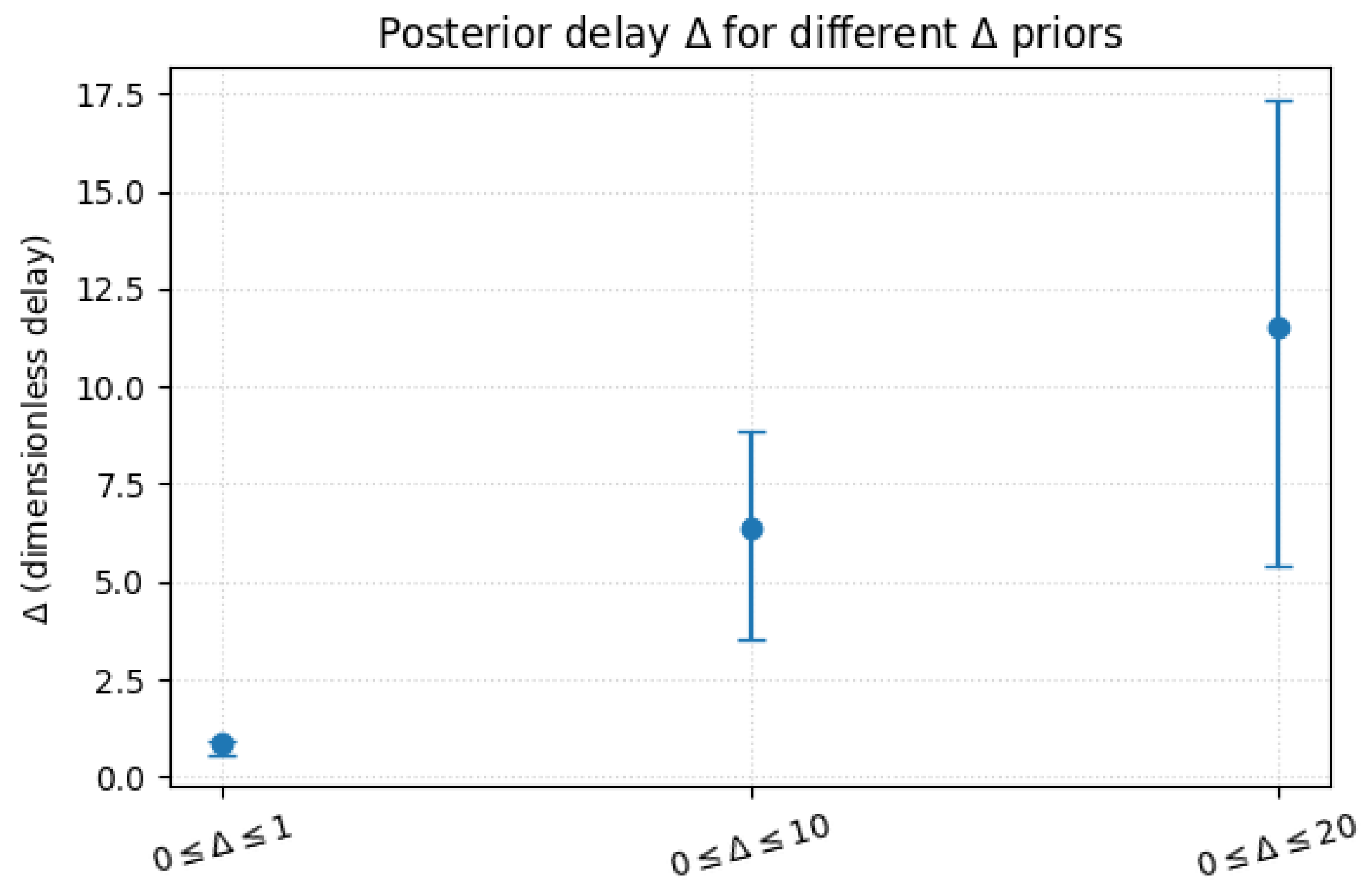
Posterior constraints on the dimensionless delay parameter for three different flat priors on the allowed delay range. Points mark the posterior medians, with vertical bars showing the corresponding uncertainties. The trend illustrates that current data favour a nonzero delay but do not yet place a sharp upper bound on .
Figure A6.
Posterior constraints on the dimensionless delay parameter for three different flat priors on the allowed delay range. Points mark the posterior medians, with vertical bars showing the corresponding uncertainties. The trend illustrates that current data favour a nonzero delay but do not yet place a sharp upper bound on .
References
- Peebles, P.J.E. Principles of Physical Cosmology; Princeton University Press: Princeton, 1993. [Google Scholar]
- Weinberg, S. Cosmology; Oxford University Press: Oxford, 2008. [Google Scholar]
- Aghanim, N.; et al. Planck 2018 results. VI. Cosmological parameters. Astronomy & Astrophysics 2020, arXiv:1807.06209641, A6. [Google Scholar]
- Koivisto, T.S. Dynamics of nonlocal cosmology. Physical Review D 2010, 82, 123516, example of nonlocal / non-Markovian cosmology. [Google Scholar]
- Woodard, R.P. Nonlocal Models of Cosmic Acceleration. Foundations of Physics 2014, 44, 213–233. [Google Scholar] [CrossRef]
- Barrow, J.D. Sudden future singularities. Classical and Quantum Gravity 2004, 21, L79–L82, representative of nonstandard late-time dynamics. [Google Scholar] [CrossRef]
- Atalebe, S. Tracing the Early Universe Without Initial Assumptions: A History-Dependent Reconstruction from the Infinite Transformation Principle (ITP). Preprints 2025. Preprint, Infinite Transformation Principle early-universe reconstruction. [Google Scholar] [CrossRef]
- Moresco, M.; et al. Improved constraints on the expansion rate of the Universe up to z∼1.1 from the spectroscopic evolution of cosmic chronometers. Journal of Cosmology and Astroparticle Physics 2012, 2012, 006. [Google Scholar] [CrossRef]
- Alam, S.; et al. The clustering of galaxies in the completed SDSS-III Baryon Oscillation Spectroscopic Survey: Cosmological analysis of the DR12 galaxy sample. Monthly Notices of the Royal Astronomical Society 2017, 470, 2617–2652. [Google Scholar] [CrossRef]
- Blake, C.; et al. The WiggleZ Dark Energy Survey: The growth rate of cosmic structure since redshift z=0.9. Monthly Notices of the Royal Astronomical Society 2011, 415, 2876–2891. [Google Scholar] [CrossRef]
- Betoule, M.; et al. Improved cosmological constraints from a joint analysis of the SDSS-II and SNLS supernova samples. Astronomy & Astrophysics 2014, 568, A22, JLA compilation. [Google Scholar] [CrossRef]
- Guth, A.H. Inflationary universe: A possible solution to the horizon and flatness problems. Physical Review D 1981, 23, 347–356. [Google Scholar] [CrossRef]
- Linde, A.D. A new inflationary universe scenario: A possible solution of the horizon, flatness, homogeneity, isotropy and primordial monopole problems. Physics Letters B 1982, 108, 389–393. [Google Scholar] [CrossRef]
- Baumann, D. TASI Lectures on Inflation. In Physics of the Large and the Small; Csáki, C., Dodelson, S., Eds.; TASI 2009, World Scientific, 2011. [Google Scholar]
- Steinhardt, P.J.; Turok, N. A Cyclic Model of the Universe. Science 2002, 296, 1436–1439. [Google Scholar] [CrossRef] [PubMed]
- Lehners, J.L. Ekpyrotic and cyclic cosmology. Physics Reports 2008, 465, 223–264. [Google Scholar] [CrossRef]
- Jimenez, R.; Loeb, A. Constraining cosmological parameters based on relative galaxy ages. The Astrophysical Journal 2002, 573, 37–42. [Google Scholar] [CrossRef]
- Eisenstein, D.J.; et al. Detection of the Baryon Acoustic Peak in the Large-Scale Correlation Function of SDSS Luminous Red Galaxies. The Astrophysical Journal 2005, 633, 560–574. [Google Scholar] [CrossRef]
- Perlmutter, S.; et al. Measurements of Ω and Λ from 42 High-Redshift Supernovae. The Astrophysical Journal 1999, 517, 565–586. [Google Scholar] [CrossRef]
- Riess, A.G.; et al. Observational evidence from supernovae for an accelerating universe and a cosmological constant. The Astronomical Journal 1998, 116, 1009–1038. [Google Scholar] [CrossRef]
- Chen, Y. Constraints on the Hubble constant using cosmic chronometers and other cosmological probes. Journal of Cosmology and Astroparticle Physics 2019. Representative recent H(z) / H0 analysis; update details as needed. [Google Scholar]
- Battefeld, D.; Peter, P. A Critical Review of Classical Bouncing Cosmologies. Physics Reports 2015, 571, 1–66. [Google Scholar] [CrossRef]

Table 1.
Two bin ITP fits with different priors on the delay parameter . Values are posterior medians with asymmetric credible intervals. Broad priors () deliver stable background parameters and increasingly long delays, whereas the short delay run () drives to the prior ceiling and distorts .
Table 1.
Two bin ITP fits with different priors on the delay parameter . Values are posterior medians with asymmetric credible intervals. Broad priors () deliver stable background parameters and increasingly long delays, whereas the short delay run () drives to the prior ceiling and distorts .
| prior | ||||
|---|---|---|---|---|
Table 2.
Comparison of representative ITP fits to the combined dataset. Quoted values are posterior medians with asymmetric credible intervals. The fiducial two–bin run with a broad delay prior recovers a long–memory solution with conventional background parameters. Forcing the same model into a short–delay regime () drives to the prior ceiling and distorts . The five–parameter run independently reproduces the preference for a long delay while keeping in a similar range.
| Run | Non-Markovian amplitude(s) | |||
|---|---|---|---|---|
| Two–bin ITP (fiducial) | ||||
| Two–bin ITP (short–delay test) | ||||
| Five–parameter ITP (early universe) |
Table 3.
Joint constraints for the baseline CDM and five–parameter ITP models.
| Model | [km s Mpc] | ||
|---|---|---|---|
| CDM | 18.84 | ||
| ITP | 19.08 |
Disclaimer/Publisher’s Note: The statements, opinions and data contained in all publications are solely those of the individual author(s) and contributor(s) and not of MDPI and/or the editor(s). MDPI and/or the editor(s) disclaim responsibility for any injury to people or property resulting from any ideas, methods, instructions or products referred to in the content. |
© 2026 by the authors. Licensee MDPI, Basel, Switzerland. This article is an open access article distributed under the terms and conditions of the Creative Commons Attribution (CC BY) license (http://creativecommons.org/licenses/by/4.0/).
Copyright: This open access article is published under a Creative Commons CC BY 4.0 license, which permit the free download, distribution, and reuse, provided that the author and preprint are cited in any reuse.


