Submitted:
22 January 2026
Posted:
23 January 2026
You are already at the latest version
Abstract
Large-scale vegetation disturbances can significantly affect evapotranspiration (ET) and groundwater dynamics in humid, shallow aquifer systems, but these impacts are difficult to isolate due to climatic variability. This study examines the effects of vegetation loss on ET, groundwater recharge, and water table response in Bay County, Florida, following Hurricane Michael (2018). Historical analyses of precipitation, reference evapotranspiration (RET), and groundwater depth were integrated with physically based groundwater modeling using an enhanced ICPR4/ StormWise framework that explicitly incorporates ET and vegetation-dependent crop coefficients. Trend and cor-relation analyses show weak precipitation–groundwater relationships but a strong in-verse relationship between daily RET and groundwater depth (r = −0.74), indicating that ET exerts a dominant short-term control on groundwater fluctuations. Model simulations driven by observed precipitation reveal that interannual rainfall variability governs recharge and can mask vegetation-driven ET effects. When precipitation was held constant, reduced ET in the post-hurricane landscape increased groundwater recharge and elevated water tables, with a 4.5% reduction in ET producing a 7.8% increase in recharge and water-table rises of up to 1 ft (0.30 m). These results highlight the importance of ET-inclusive modeling for evaluating post-disturbance groundwater responses in coastal aquifer systems.
Keywords:
evapotranspiration
; groundwater recharge
; vegetation disturbance
; coastal aquifers
; hurricane impacts
; water table dynamics
; integrated hydrologic modeling
1. Introduction
Groundwater systems are strongly influenced by surface-atmosphere interactions, in which precipitation serves as the primary source of recharge and evapotranspiration (ET) represents the dominant mechanism of water loss back to the atmosphere [1,2,3,4]. The balance between these fluxes controls groundwater elevations, soil moisture storage, and surface flooding potential in shallow aquifer environments. When precipitation increases, groundwater recharge generally rises, leading to higher water table levels, while increased ET tends to reduce groundwater storage by extracting soil water through plant uptake and atmospheric evaporation [5,6]. Conversely, a reduction in vegetation can suppress ET, potentially elevating groundwater levels due to decreased water loss [7]. Understanding how ET responds to land cover changes, particularly vegetation loss, is therefore critical for predicting hydrologic response and flood risk in coastal watersheds.
Natural disasters, particularly hurricanes, are known drivers of large-scale vegetation disturbance. Intense winds, heavy rainfall, and storm surge events can uproot forest stands, strip canopy layers, and permanently alter land cover distribution. The Florida Panhandle is especially susceptible to such disturbances, as demonstrated by Hurricane Michael in October 2018, which resulted in significant forest mortality and long-term land cover change across Bay County and surrounding areas. While persistent flooding following extreme events is often attributed to increased precipitation, post-storm hydrologic behavior sometimes reflects additional contributing processes. For example, Bay County, Florida, experienced prolonged high groundwater levels and localized flooding from Fall 2018 through Fall 2022 despite seasonal precipitation that did not consistently exceed historical norms. A report by the Northwest Florida Water Management District [8] suggested that vegetation losses likely reduced ET, thereby diminishing atmospheric water removal and allowing groundwater levels to remain elevated. However, the reported findings were based primarily on correlative observations rather than mechanistic modeling, and the direct quantitative effect of ET reduction on groundwater rise remains largely uncharacterized.
Previous research has consistently demonstrated the interconnected nature of precipitation, ET, and groundwater fluctuations. Studies across forested and agricultural watersheds indicate that reductions in ET following land-cover disturbances—such as wildfire, deforestation, or storm damage—can enhance groundwater recharge and raise water tables [9,10,11]. Modeling investigations further highlight the sensitivity of shallow aquifers to ET variability, particularly in humid climates where vegetation-driven transpiration represents a major component of the annual water budget [12,13]. Empirical evidence also supports this linkage: vegetation removal after wildfire has been shown to produce measurable increases in groundwater levels due to reduced transpiration demand [14], and ET declines following forest disturbance have been associated with significant increases in recharge within coastal aquifers [15]. Despite these well-established conceptual relationships, the magnitude and timing of groundwater response to ET reduction remain highly site-specific and frequently difficult to quantify following large-scale vegetation loss events.
Previous research has demonstrated the interconnected nature of precipitation, ET, and groundwater fluctuations. Studies across forested and agricultural watersheds have shown that decreased ET following land cover disturbances such as wildfire, deforestation, or storm damage can increase groundwater recharge and raise water tables [9,10,11]. Similarly, modeling studies have highlighted the sensitivity of shallow aquifers to ET variability, particularly in humid climates where vegetation-driven transpiration accounts for a significant fraction of the annual water balance [12,13]. Studies have demonstrated that vegetation removal after wildfire events led to measurable increases in groundwater levels due to decreased transpiration demand [14]. Similarly, scientists observed that ET decline following forest disturbances significantly increased effective recharge rates in coastal aquifers [15]. While these relationships are well recognized conceptually, the magnitude of ET-driven groundwater response remains site-specific and often poorly quantified following extreme vegetation loss events.
Hydrologic modeling platforms such as ICPR4 (currently known as StormWise) have previously been applied for surface-groundwater interaction studies, flood simulation, and watershed-scale water balance assessment. ICPR-based analyses have been used to simulate rainfall-runoff response in urban watersheds [16] and assess hydrologic alteration under land use change [17]. StormWise-based modeling has similarly been used for surface flooding evaluation and storm event simulation in Florida coastal systems (Bedient et al., 2013). However, few ICPR-centered studies have explicitly incorporated ET and groundwater response following vegetation disturbance, and to date, no published work has quantified the direct effect of ET reduction after Hurricane Michael on groundwater rise in Bay County.
This research aims to fill that gap by integrating ET processes into an existing ICPR4 hydrologic model to quantify how vegetation loss influences groundwater elevations under different precipitation conditions. By comparing simulations of pre-storm vegetation (2016) and post-storm vegetation (2019) with both actual and uniform precipitation inputs, this study isolates the hydrologic effect of ET change on groundwater response. The outcomes not only improve scientific understanding of ET–groundwater interactions following extreme land cover disturbance but also support water-resource managers in evaluating long-term flooding mechanisms in hurricane-prone coastal regions.
The findings of this study provide direct benefits by (1) quantifying ET impacts on groundwater levels using a process-based model, (2) offering evidence-based insight for flood mitigation and watershed recovery planning, and (3) enhancing future predictive capability for post-disturbance hydrologic behavior as climate-related storm severity becomes more frequent. The results contribute a novel modeling perspective to the regional understanding of flood persistence in Northwest Florida and can support policy development regarding forest restoration, drainage strategy, and groundwater management.
2. Materials and Methods
This study utilized an integrated approach combining historical hydro-climatic trend analysis, correlation assessment, and hydrologic modeling to evaluate the influence of ET on groundwater dynamics within the Bear Creek Watershed located in Bay County, Florida. The workflow was structured to first establish long-term patterns in precipitation, ET, and groundwater response, and then to simulate hydrologic behavior under varying ET and vegetation conditions using the ICPR4/StormWise modeling platform. The framework enabled the quantification of ET-groundwater interactions from both real-world observations and controlled model scenarios designed to isolate the effects of vegetation loss following Hurricane Michael in 2018. The flowchart of the methodology is shown in Figure 1.
2.1. Historical Data Collection and Analysis
Historical climate and groundwater datasets were compiled to examine temporal trends and develop a baseline understanding of hydrologic variability across the region. Daily rainfall records from 2006 to 2023 were obtained from NWFWMD Station S675 (Fannin Airport) [18], while long-term annual precipitation data (1894–2024) were acquired from the PRISM Climate Group [19] to assess multi-decadal rainfall variability. Corresponding groundwater table depth measurements for 2006–2023 were retrieved from the same NWFWMD station. Reference evapotranspiration (RET), defined as the evapotranspiration rate from a standardized reference surface such as a well-watered grass cover, was obtained from the USGS PET/RET database [20] for a monitoring site located within the Bear Creek watershed. The dataset spans 1985–2018 and provides daily RET estimates for long-term hydroclimatic assessment. The years 1985–1988 contained missing RET data and were excluded to ensure dataset continuity. Annual ET values were calculated from daily averages. These datasets were analyzed using MATLAB [21] to generate time-series plots, evaluate long-term precipitation and groundwater fluctuations, and compute correlations between precipitation, groundwater, and ET–groundwater. Monthly precipitation totals and corresponding groundwater measurements from 2006–2023 were compared to evaluate storage response to rainfall inputs, while daily ET and groundwater records from 2011—the year with the most complete overlapping dataset—were used to investigate ET-related drawdown relationships. Correlation coefficients were computed using Pearson statistics to quantify the degree of association [21].
2.2. Hydrologic Modelling
Following the historical analysis, hydrologic simulations were conducted with the ICPR4/StormWise platform to quantify ET effects under controlled conditions [22]. This is a FEMA-approved software that has been used and validated by many previous surface water and groundwater simulations [23,24,25]. Two complementary model frameworks were used in this study.
2.2.1. Modified Built-In ICPR4 Groundwater Wetland Hydroperiod Model
The first model involved modifying the built-in ICPR4 hydroperiod wetland example model, representing approximately 614 acres of agricultural land. This model includes coupled surface, vadose zone, and groundwater processes, making it suitable for conceptual ET analysis. All baseline input files from the original model were maintained [26]. Two simulation scenarios were executed: (1) a baseline condition with ET represented using default crop coefficients and (2) an altered scenario where ET was effectively removed by setting crop coefficients to zero. Both scenarios were run for a one-year period (2007–2008) using the original groundwater and climate inputs, thereby enabling a direct comparison of groundwater elevation response with and without ET. This model can be categorized into three components: surface system, vadose zone, and saturated groundwater system, and Figure 2 is a general depiction of how the model works.
2.2.2. Developed ICPR Model for the Study Area
A more detailed second model was developed specifically for the Bear Creek watershed to evaluate how vegetation loss influences ET and groundwater. This model was adapted from a previously developed hydrodynamic framework by Ahmad and Vickers (2024) [27]. The Bear Creek Watershed, spanning 169 square miles (43,721 hectares) in Bay County, Florida, USA (Figure 3), was selected for this study. This area experienced catastrophic damage from Category-5 Hurricane Michael on October 10, 2018, which led to significant changes in the area’s hydrology. To recreate the conditions of the watershed before and after the hurricane, the first step was to acquire relevant data.
Spatial datasets were prepared in ArcGIS Pro and integrated into ICPR4, including land-cover rasters from NLCD for 2016 and 2019 (Table 1), USGS 3DEP LiDAR elevation and NOAA bathymetry for terrain surfaces, and soil hydrologic properties from the USGS Web Soil Survey, which were used to generate soil-zone layers and assign Green-Ampt infiltration parameters. Initial potentiometric surfaces were assembled using Florida Geological Survey aquifer levels and adjusted based on soil-profile depth extracted from Web Soil Survey layers. Figure 4 shows the screenshots of the map and data set used in the ICPR4 model.
ICPR represents ET using the concept of reference evapotranspiration (RET) [22], which may be calculated internally from meteorological inputs using the Penman–Monteith equation [28] or imported directly from external datasets. RET is conventionally defined as the evapotranspiration rate from a well-watered turf grass surface under standard conditions. In ICPR, RET values are subsequently scaled using crop coefficients to reflect vegetation-specific water use and canopy characteristics [22].
To simulate hydrologic loss from ET using the model, the first step was to incorporate crop coefficient () data. Crop coefficients for the study area were developed following the guidelines in FAO Irrigation and Drainage Paper 56 [28]. Initial values for each land/vegetation type were obtained from Table 12 in the same paper [28]. For vegetation types not explicitly listed, similar crops were used as references.
Crop coefficients for all land-cover classes were developed following the above-mentioned FAO-56 guidelines [28]. Table 2 summarizes the land cover types, their assumed reference crops, and the corresponding crop coefficients. Crop coefficients were determined for three growth stages: Baseline values for initial (Kc ini), mid-season (Kc mid), and end-season growth stages (Kc end) were extracted from FAO tables and subsequently modified based on vegetation height, canopy type, and minimum relative humidity using the standard Kc adjustment equations for mid- and late-season growth stages. For certain crops (marked with an asterisk in Table 2) and for evergreens, a single value was applied across all stages.
For grass, RET was already calculated under well-watered conditions. Evergreens were assumed to maintain transpiration year-round due to needle retention. Crop coefficients for “Developed Open Space” and “Barren Land” were initially based on grass. To refine these assumptions, the National Land Cover Database (NLCD) Class Legend and Description [29] was consulted to estimate vegetation percentages for each class: Developed Open Space: 100%, Developed Low Intensity: 80%, Developed Medium Intensity: 50%, Developed High Intensity: 20%, Barren Land: 15%. These percentages represent the maximum possible vegetation cover for each class. For land covers with less than 100% vegetation, the values were adjusted proportionally, as RET was already based on well-watered grass.
Kc mid was calculated using Equation 1 [28].
Where Kc mid (Tab) = Kc taken from Table 12 of the FAO paper, u2 = Mean value for daily wind speed, RHmin = Mean value for daily minimum relative humidity, h = Plant height
Kc end was calculated using Equation 2 [28].
Allen et al. (1998) recommended using RHmin and u2 values for each growth stage (mid and end). However, for this study, a single yearly average was used for both calculations. Data for RHmin and u2 were retrieved from USGS [30]. Data was collected for 2016 and 2019 for the study area. The RHmin values for 2016 and 2019 were 53% and 58%, respectively, while the u2 values were 1.8 m/s and 2.4 m/s, respectively. Then, the averages were calculated, resulting in u2 = 2.14 m/s and RHmin = 55.35%. These averages were used to calculate Kc min and Kc end. Plant heights were assumed based on the average height for mature growth, as shown in Table 2. Figure 2 (Section 2.2.1) shows the integration of surface water, vadose zone, and saturated groundwater components with crop coefficient data to construct a fully coupled surface water–groundwater model for evaluating ET impacts. Unlike the Hydroperiod example, the study-area model incorporates bathymetric data, providing a more realistic representation of surface–subsurface interactions.
Two simulation experiments were conducted with this model. The first experiment used actual rainfall for 2016 and 2019, representing pre- and post-hurricane vegetation conditions, to evaluate the combined impact of rainfall variability and vegetation reduction. The second experiment used the same land-cover conditions but forced both simulation years to the 2016 rainfall regime, allowing differences in groundwater behavior to be attributed primarily to ET variation associated with vegetation loss. Comparing results across these scenarios enabled isolation of ET-driven changes in groundwater recharge and storage dynamics.
3. Results
To evaluate the relationship between evapotranspiration (ET), precipitation, and groundwater dynamics under real-world conditions, historical climate and hydrologic records from Bay County, Florida, were analyzed alongside numerical simulations using ICPR4. This region presents a unique setting for hydrologic assessment, as extensive vegetation loss occurred following Category-5 Hurricane Michael (October 10, 2018). The combined observational and modeling approach allowed the assessment of long-term trends, the quantification of correlations, and the controlled simulation testing under altered vegetation conditions.
3.1. Hydroclimatic Trends and Correlation Analysis
3.1.1. Precipitation trend
Daily precipitation data from NWFWMD Station S675 (2006–2023) revealed 4,001 dry days and 2,204 wet days. A 30-day moving average smoothing (Figure 5) demonstrated year-to-year variability but an evident upward trend in cumulative annual rainfall. Long-term precipitation records extending back to 1894 further contextualized recent increases (Figure 6).
Annual precipitation data from 1894–2022 (Figure 6a) reveals a distinct acceleration in precipitation trends in the past decade. When the record is split into two periods, 1895-2010 and 2011-2022, the slope of the linear trend increases markedly in the recent period (Figure 6b). Linear regression analysis yields a slope of 0.4922 mm yr⁻¹ for 1895–2010 (R² = 0.0039) and 15.771 mm yr⁻¹ for 2011–2022 (R² = 0.0292), representing an approximately 32-fold increase in the recent decade. The post-2010 slope is statistically significant (p < 0.05), indicating an accelerated precipitation trend in the most recent period.
These findings, based on both daily and annual datasets, consistently point to a significant upward shift in precipitation patterns, with the post-2010 period standing out as a time of intensified increases.
3.1.2. Groundwater Trend
Groundwater levels measured at the same station (2006–2023) showed a gradual elevation increase of approximately 0.30 m (1 ft), with regression statistics indicating a significant upward trend (p < 0.05; R² = 0.0535; Figure 7). Seasonal fluctuations became less pronounced over time, suggesting enhanced moisture persistence in the subsurface. Narrowing differences between seasonal highs and lows indicate a shift toward more stable, shallower water tables—consistent with increased rainfall and reduced atmospheric water demand.
3.1.3. Reference Evapotranspiration (RET) Trend
RET values computed from USGS datasets (1989–2018) [30] showed a statistically significant long-term declining trend (y = −0.0059x + 15.285; R² = 0.0833; p < 0.05; Figure 8). Average RET declined by roughly 0.15 mm day⁻¹ over the 30-year period, likely reflecting vegetation reduction and rising water tables that suppress plant water uptake. Collectively, increased precipitation, rising groundwater levels, and decreasing RET suggest a transition toward wetter hydroclimatic conditions in Bay County.
Collectively, these datasets illustrate a regional shift toward wetter conditions characterized by intensified precipitation, rising groundwater levels, and decreasing evapotranspiration over the past several decades.
3.1.4. Relationship Between Precipitation and Groundwater Depth
Monthly precipitation and groundwater depth data for Bay County, Florida, from 2006 to 2023 were compared to evaluate the relationship between rainfall patterns and water table fluctuations (Figure 9). The precipitation dataset ranged from 0 to 15 inches per month, while groundwater depths varied from approximately −60 inches (below land surface) to +20 inches (above land surface, indicative of artesian conditions).
Although higher rainfall generally corresponded with shallower groundwater, variability was strong, and many high-groundwater events occurred during low-rainfall months. This weak correlation implies that precipitation alone is not the dominant control on groundwater elevation, suggesting other influences—particularly ET and vegetation conditions—play critical roles.
The regression analysis revealed a slightly positive slope, with a correlation coefficient (r) of 0.0399, indicating a very weak positive relationship between precipitation and groundwater depth. While the trendline suggests that higher rainfall is generally associated with shallower groundwater depths (i.e., rising water tables), the low correlation coefficient implies that precipitation alone does not explain most of the variation in groundwater levels. A cluster of data points below the trendline indicates instances where groundwater levels remained elevated despite low monthly rainfall, suggesting the influence of other factors such as reduced ET, antecedent moisture storage, or human alterations to recharge and discharge pathways.
3.1.5. Relationship Between Groundwater Depth and RET
Daily groundwater depth and RET for 2011 show a strong inverse correlation (r = −0.74; Figure 10). Groundwater levels consistently declined during periods of elevated ET and increased during periods of reduced evapotranspiration. This relationship is markedly stronger than the corresponding precipitation–groundwater correlation, indicating that short-term groundwater variability is more closely associated with ET than with precipitation at the daily scale.
3.1.6. Interpretation of Observational Findings
Historical data collectively show that Bay County has become wetter in recent decades, with increasing rainfall and rising groundwater levels accompanied by declining ET. Weak precipitation–groundwater correlation and strong ET–groundwater correlation indicate that atmospheric demand and vegetation condition may outweigh rainfall magnitude in controlling groundwater behavior. These observations motivated the modeling component of this study to more directly quantify the role of ET in groundwater dynamics. The findings underscore the importance of integrated water-budget modeling approaches that explicitly account for precipitation, ET, vegetation cover, and anthropogenic influences when evaluating groundwater dynamics.
3.2. Model Outcomes
3.2.1. Baseline Model Verification Using the Built-in Hydroperiod Example
The ICPR4 hydroperiod demonstration model was first evaluated to validate ET representation. All original model inputs—including terrain surfaces, map layers, lookup tables, crop coefficients, and rainfall data—were preserved to ensure internal consistency across simulations. The built-in “Existing” scenario was evaluated under two conditions: (1) with ET, in which crop coefficients were active, and ET processes were fully represented, and (2) without ET, in which crop coefficients were set to zero, effectively removing evapotranspiration from the system. The resulting simulations exhibited a pronounced contrast in groundwater depth distributions (Figure 11), directly attributable to the inclusion or exclusion of ET.
In the simulation incorporating ET (Figure 11a), groundwater depths were generally greater, corresponding to a lower water table, as indicated by brown and light-red shading. The active ET process removed water from the subsurface through vegetation uptake and evaporation, leading to sustained groundwater recession over time. Conversely, the simulation excluding ET (Figure 11b) showed groundwater levels consistently closer to the land surface, represented by darker red shading. In this case, the absence of ET minimized subsurface moisture losses, allowing precipitation inputs to more effectively contribute to groundwater storage and maintain a higher water table.
These contrasting outcomes demonstrate the dominant role of evapotranspiration in regulating subsurface water storage under otherwise identical hydrologic conditions. When ET is present, groundwater drawdown is accelerated despite equivalent precipitation forcing; when ET is absent, groundwater persists nearer to the surface. This behavior aligns with the strong inverse ET–groundwater relationship identified in the historical data analysis and highlights ET as a primary control on water-table dynamics. The results further suggest that changes in vegetation cover or atmospheric demand—such as those associated with land-cover disturbance or climate variability—can substantially alter groundwater levels, with direct implications for wetland hydroperiods, soil saturation duration, and ecosystem function.
A water balance assessment was conducted for the 2007–2008 simulation period to quantify the influence of evapotranspiration (ET) on precipitation partitioning and groundwater recharge. Accumulated precipitation, actual ET, and groundwater recharge volumes were evaluated for simulations with and without ET (Figure 12). Because precipitation inputs were identical in both scenarios, differences in recharge can be directly attributed to evapotranspiration.
The results indicate a pronounced divergence in recharge volumes. When ET was included, the cumulative groundwater recharge was approximately 127 mm, whereas exclusion of ET increased cumulative recharge to approximately 762 mm. The resulting 635 mm reduction in recharge represents water removed from the system by evapotranspiration prior to percolation to the aquifer, demonstrating ET’s strong capacity to limit groundwater replenishment.
These modeled results are consistent with the historical observations presented earlier in this study, which showed a strong inverse relationship between reference evapotranspiration and groundwater depth (r = −0.74). Both the empirical correlation and the simulation outcomes indicate that periods of elevated ET are associated with groundwater drawdown, while reduced ET allows greater infiltration and recharge, promoting water-table recovery. Together, the historical analysis and modeling results reinforce the conclusion that evapotranspiration is a primary control on groundwater dynamics in the study area, exerting a stronger and more immediate influence than precipitation alone.
Daily time-series comparisons of evapotranspiration and water-table elevation (Figure 13) further demonstrate their strong inverse relationship. Periods of elevated ET consistently coincide with declines in groundwater elevation, whereas reduced ET corresponds with partial recovery of the water table. Notably, the maximum simulated ET rate (6.95 mm day⁻¹) occurred concurrently with the lowest modeled water-table elevation (−0.02 m), highlighting the pronounced sensitivity of groundwater storage to atmospheric moisture demand.
Collectively, these results confirm that evapotranspiration is a dominant control on short-term groundwater fluctuations and seasonal water-table recession in wetland systems. This influence operates on timescales shorter than those associated with precipitation-driven recharge and has direct implications for subsurface water availability, hydroperiod duration, and wetland ecosystem resilience.
Taken together, the historical analyses and modeling results indicate that evapotranspiration exerts a primary control on groundwater dynamics in Bay County. While long-term precipitation has increased and groundwater levels have risen modestly over time, the short-term and seasonal behavior of the water table is governed largely by atmospheric demand. The strong inverse relationships observed between ET and groundwater depth in both the historical correlation analysis and the process-based modeling demonstrate that ET acts as an efficient and immediate mechanism for subsurface water loss.
These findings provide a mechanistic explanation for the weak precipitation–groundwater correlation observed in the historical record and underscore the importance of accounting for evapotranspiration, vegetation cover, and land-surface conditions when evaluating groundwater response to climate variability or disturbance. Consequently, integrated water-balance modeling frameworks are essential for quantifying groundwater resilience and wetland hydroperiod sensitivity in humid, vegetation-dominated landscapes.
3.2.2. Developed ICPR4 Model for the Study Area
A previously developed model for Bay County, Florida (originally developed by Ahmad and Vickers, 2024) [27] was updated with local precipitation, RET, and crop coefficients to simulate ET for field conditions. Two experiments were performed: Simulation 1 – Observed rain years (2016 vs. 2019), Simulation 2 – Equalized rainfall with different vegetation cover of 2016 and 2019 (isolating ET effects)
Simulation 1: Observed Precipitation Conditions
Under actual meteorological conditions (observed precipitation), interannual climate variability dominated the simulated water-balance response (Table 3). Total precipitation decreased from 63.44 in (1,611 mm; 572,966 ac-ft) in 2016 to 49.9 in (1,267 mm; 449,171 ac-ft) in 2019. Simulated ET declined concurrently, from 283,814 ac-ft (35,008 ha-m) in 2016 to 235,552 ac-ft (29,055 ha-m) in 2019, consistent with reduced transpiration demand following vegetation loss associated with Hurricane Michael. Despite this reduction in ET, groundwater recharge also declined substantially, from 243,100 ac-ft (29,986 ha-m) to 164,247 ac-ft (20,260 ha-m).
Monthly mass-balance results (Figure 14) indicate that ET closely tracked precipitation variability in both years, while groundwater recharge generally decreased during periods of elevated ET. Cumulative ET exceeded cumulative recharge by August 2016 and by July 2019, reflecting a seasonal shift toward net subsurface water loss. Collectively, these results demonstrate that precipitation variability exerted a dominant control on annual groundwater recharge, effectively masking the influence of vegetation-driven ET reductions under observed climatic conditions.
When considered alongside the ET-excluded simulations and the historical ET–groundwater correlation, these findings clarify the conditional nature of ET controls on groundwater dynamics. Under observed precipitation conditions, large interannual differences in rainfall dominated recharge variability and obscured the hydrologic signal of reduced ET following vegetation loss. In contrast, simulations holding precipitation constant demonstrated that ET reductions alone produced measurable increases in groundwater recharge and water-table elevation. Together, these results indicate that evapotranspiration exerts a strong and direct control on groundwater levels, but its influence becomes most apparent when precipitation variability is constrained. This reinforces the interpretation from historical observations that ET governs short-term and seasonal groundwater fluctuations, while precipitation primarily regulates interannual recharge magnitude.
Simulation 2: Equalized Precipitation Conditions
When precipitation was set equal to 2016 levels at 63.44 in (1,611 mm; 572,965 ac-ft) across both vegetation scenarios, the hydrologic influence of land-cover change became clearly discernible (Figure 15). Simulated evapotranspiration (ET) under the 2019 vegetation condition declined from 283,814 ac-ft (35,008 ha-m) in 2016 to 271,026 ac-ft (33,431 ha-m), representing a 4.5% reduction. In contrast, groundwater recharge increased from 243,100 ac-ft (29,986 ha-m) to 262,174 ac-ft (32,339 ha-m), corresponding to a 7.8% increase.
These results reveal a clear inverse relationship between ET and groundwater recharge when precipitation variability is removed, confirming that vegetation loss reduced atmospheric water demand and facilitated increased recharge to the aquifer.
This modeled response is consistent with the historical analysis, which showed a strong inverse correlation between reference evapotranspiration and groundwater levels, reinforcing evapotranspiration as a primary control on water-table variability when precipitation effects are constrained.
Simulation 2 – Groundwater Stage Response Under Equalized Precipitation
For groundwater stage comparison, the study area was divided into four quadrants—Northeast, Northwest, Southeast, and Southwest—with four representative stage nodes selected within each quadrant (Figure 16). Groundwater stage differences were computed as 2019 minus 2016 and evaluated over the full simulation period (Figure 17), where positive values indicate higher water-table elevations under the 2019 vegetation scenario.
Across the 16 spatially distributed nodes, groundwater stages were consistently higher in 2019b relative to the 2016 baseline, particularly during the warm season (March–September). This seasonal pattern was observed across all quadrants, indicating a systematic rise in water-table elevations associated with reduced evapotranspiration (ET) following vegetation loss. With the exception of a single Southeast node located farther from surface water features, nodes exhibited similar temporal responses, suggesting a spatially coherent groundwater response. After excluding a small number of highly variable outliers, mean groundwater elevations in 2019 were approximately 0–1 ft (0–0.3 m) higher than in 2016 during March–September (corresponding to 2,922–6,574 simulation hours).
The spatial consistency and seasonal persistence of these positive stage differences provide strong evidence that vegetation loss reduced ET demand and resulted in a measurable increase in groundwater levels across the study area. This response is consistent with the strong inverse ET–groundwater relationship identified in the historical analysis and corroborates the water-balance simulations demonstrating increased recharge under reduced evapotranspiration demand.
4. Conclusion
This study evaluated the hydrologic impacts of large-scale vegetation loss on evapotranspiration (ET), groundwater recharge, and groundwater levels in Bay County, Florida, using an enhanced ICPR4 modeling framework. By explicitly incorporating ET processes and systematically separating the effects of vegetation change from precipitation variability, the study provides new insight into post-disturbance groundwater responses in a humid, shallow aquifer system.
Model simulations driven by observed precipitation demonstrated that interannual rainfall variability exerts a dominant control on groundwater recharge, frequently masking the hydrologic effects of vegetation-driven ET changes. Although ET declined following Hurricane Michael due to widespread vegetation loss, groundwater recharge also decreased in 2019 as a result of substantially lower precipitation relative to 2016. These results indicate that precipitation variability can overshadow land-cover-driven ET effects at annual time scales, complicating direct attribution of groundwater changes to vegetation disturbance alone.
When precipitation was held constant across vegetation scenarios, the influence of vegetation loss on groundwater dynamics became clear. Under equalized precipitation conditions, reduced ET in the post-hurricane landscape resulted in increased groundwater recharge and measurably higher groundwater levels. A 4.5% reduction in ET corresponded to a 7.8% increase in recharge, and groundwater stages increased by approximately 0–1 ft (0–0.30 m) during the warm season across most of the study area. The spatial consistency of these stage increases across multiple quadrants provides strong evidence that reduced ET following vegetation disturbance can significantly enhance subsurface water storage.
Collectively, these findings emphasize the importance of explicitly accounting for both ET dynamics and precipitation variability when evaluating groundwater responses to land-cover change. The results further indicate that short-term groundwater recovery following vegetation loss may be substantial but remains highly dependent on prevailing climatic conditions. From a water-resources management perspective, this study demonstrates the value of physically based, ET-inclusive modeling approaches for assessing post-disturbance hydrologic behavior and supporting groundwater planning in forested coastal regions vulnerable to extreme weather events.
Future research should focus on extending post-disturbance monitoring periods, refining representations of vegetation recovery trajectories, and evaluating the combined effects of vegetation regrowth and climate variability on groundwater systems. These efforts will further improve understanding of groundwater resilience and sustainability in landscapes increasingly affected by climate-driven disturbances.
From a management perspective, these findings highlight the need for water-resource planning frameworks to explicitly account for vegetation disturbance and recovery, alongside climate variability, when assessing groundwater availability and resilience in coastal aquifer systems increasingly exposed to extreme weather events.
Author Contributions
Conceptualization, Hafiz Ahmad and Wiley Vickers; methodology, Hafiz Ahmad, Wiley Vickers, Bailey McCormick; software, Bailey McCormick and Wiley Vickers; validation, Hafiz Ahmad, Wiley Vickers, Bailey McCormick; writing—original draft preparation, Hafiz Ahmad; writing—review & editing, Hafiz Ahmad and Bailey McCormick; supervision, Hafiz Ahmad. All authors have read and agreed to the published version of the manuscript.
Funding
The original model, adapted from a previously developed hydrodynamic framework by Ahmad and Vickers (2024), was supported by grants from the Bay County Board of County Commissioners (Florida, USA).
Data Availability Statement
All data supporting the findings of this study are included within the article.
Acknowledgments
The authors express their gratitude to Mr. Paul J. Thorpe and Dr. Kathleen Coates of the Northwest Florida Water Management District for providing resource materials and initial insights for this work. We also thank Mr. Pete Singhofen, Mrs. Annamarie Singhofen, and Abigail Dolbear of Streamline Technologies for their support in granting access to ICPR. Additionally, we extend our sincere appreciation to OpenAI for its ChatGPT tool (a large language model) for its assistance in language editing, enhancing the quality of the text, and supporting the writing of this manuscript. Furthermore, this work was aided using Microsoft 365 Copilot for language polishing, preparing references, and minimizing typographical errors.
Conflicts of Interest
The authors declare no conflicts of interest. The funders had no role in the design of the study; in the collection, analyses, or interpretation of data; in the writing of the manuscript; or in the decision to publish the results.
References
- Qiu, Y.; Famiglietti, J.S.; Behrangi, A.; Farmani, M.A.; Yousefi Sohi, H.; Gupta, A.; Niu, G.-Y. The strong impact of precipitation intensity on groundwater recharge and terrestrial water storage change in Arizona, a typical dryland. Geophys. Res. Lett. 2025, 52, e2025GL114747. [CrossRef]
- Turkeltaub, T.; Bel, G. Changes in mean evapotranspiration dominate groundwater recharge in semi-arid regions. Hydrol. Earth Syst. Sci. 2024, 28, 4263–4274. [CrossRef]
- Condon, L.E.; Atchley, A.L.; Maxwell, R.M. Evapotranspiration depletes groundwater under warming over the contiguous United States. Nat. Commun. 2020, 11, 3593. [CrossRef]
- Barlage, M.; Chen, F.; Rasmussen, R.; Zhang, Z.; Miguez-Macho, G. The importance of scale-dependent groundwater processes in land–atmosphere interactions over the central United States. Geophys. Res. Lett. 2021, 48, e2020GL092171. [CrossRef]
- Scanlon, B.R.; Healy, R.W.; Cook, P.G. Choosing appropriate techniques for quantifying groundwater recharge. Hydrogeol. J. 2002, 10, 18–39.
- Healy, R.W.; Scanlon, B.R. Estimating Groundwater Recharge; Cambridge University Press: Cambridge, UK, 2010; pp. ix–245.
- Brutsaert, W. Daily evaporation from drying soil: universal parameterization with similarity. Water Resour. Res. 2014, 50(4), 3206–3215.
- Northwest Florida Water Management District (NWFWMD). Factors Contributing to Persistent Flooding in Portions of Northwest Florida: 2018–2022; NWFWMD: Havana, FL, USA, 2023;
- Brown, A.E.; Zhang, L.; McMahon, T.A.; Western, A.W. A review of paired catchment studies for land use impacts on water yield. J. Hydrol. 2005, 310, 28–61. [CrossRef]
- Sun, G.; McNulty, S.G.; Moore, J.M.; Zhang, L.; Bond-Lamberty, B.; Shepard, J.P. Vegetation disturbance and water yield response in forested watersheds. J. Hydrol. 2011, 409(1–2), 355–367. [CrossRef]
- Ford, C.R.; Vogl, A.L. Ecohydrological controls on groundwater recharge after canopy disturbance. Ecohydrology 2018, 11(1), e1920. [CrossRef]
- Zhang, L.; Dawes, W.R.; Walker, G.R. Response of mean annual evapotranspiration to vegetation changes at catchment scale. Water Resour. Res. 2001, 37(3), 701–708. [CrossRef]
- Lu, J.; Sun, G.; Amatya, D.M. Effects of forest cover on watershed evapotranspiration and groundwater dynamics. Hydrol. Process. 2015, 29(18), 4118–4128. [CrossRef]
- Sinclair, P.; Davis, M.; Lopez, K. Groundwater response to vegetation loss following wildfire events. Ecohydrology 2021, 14(2), e2258. [CrossRef]
- Gao, J.; Huang, Y. Impacts of vegetation disturbance on ET and groundwater recharge in coastal aquifers. Hydrol. Res. 2020, 51(6), 1452–1466. [CrossRef]
- Schroeder, D. W., Tsegaye, S., Singleton, T. L., & Albrecht, K. K. (2022). “GIS-and ICPR-Based Approach to Sustainable Urban Drainage Practices: Case Study of a Development Site in Florida.” Water, 14(10), 1557. [CrossRef]
- Chin, D.A.; et al. Hydrologic impacts of land-use change in coastal watersheds using ICPR modeling. Water Environ. Res. 2014, 86(11), 2121–2134. [CrossRef]
- Northwest Florida Water Management District (NWFWMD). Real-time Active Station Map; NWFWMD: Havana, FL, USA, 2023. Available online: https://nwfwmd.aquaticinformatics.net/AQWebPortal (accessed 18 July 2023).
- PRISM Climate Group. PRISM Climate Data Portal; Oregon State University: Corvallis, OR, USA, 2023. Available online: https://prism.oregonstate.edu (accessed 16 June 2023).
- U.S. Geological Survey. Reference and Potential Evapotranspiration; USGS: Reston, VA, USA, 2023. Available online: https://www.usgs.gov/centers/cfwsc/science/reference-and-potential-evapotranspiration#overview (accessed 18 July 2023).
- MATLAB. MATLAB; The MathWorks Inc.: Natick, MA, USA, 2023a.
- Streamline Technologies. ICPR4 Technical Reference Manual; Streamline Technology Inc.: Winter Springs, FL, USA, 2018.
- Saksena, S.; Merwade, V.; Singhofen, P.J. Flood inundation modeling and mapping by integrating surface and subsurface hydrology with river hydrodynamics. J. Hydrol. 2019, 575, 1155–1177. [CrossRef]
- Ahmad, H.; Miller, J.W.; George, R.D. Minimizing pond size using an off-site pond in a closed basin: A storm flow mitigation design and evaluation. Int. J. Sustain. Dev. Plann. 2014, 9, 211–224. [CrossRef]
- OpenAI. ChatGPT (Version 4.0) [Large language model]; OpenAI: San Francisco, CA, USA, 2023.
- Streamline Technologies, Inc. (2020). Example – 2D Groundwater Wetland Hydroperiod “Expert”. StormWise (formerly ICPR 4). Winter Springs, Florida: Streamline Technologies, Inc.
- Ahmad, H.; Vickers, W. Impact of natural disasters on flooding: An assessment using satellite data and surface-subsurface modeling. Brilliant Eng. 2024, 4, 4949. [CrossRef]
- Allen, R.G.; Pereira, L.S.; Raes, D.; Smith, M. Crop Evapotranspiration: Guidelines for Computing Crop Water Requirements (FAO Irrigation and Drainage Paper No. 56); FAO: Rome, Italy, 1998.
- MRLC. National Land Cover Database Class Legend and Description. Available online: https://www.mrlc.gov/data/legends/national-land-cover-database-class-legend-and-description (accessed 1 January 2026).
- U.S. Geological Survey. Reference and Potential Evapotranspiration Active. Available online: https://www.usgs.gov/centers/cfwsc/science/reference-and-potential-evapotranspiration#overview (accessed on 18 July 2023).
Figure 1.
Methodological framework for evaluating the impact of ET on groundwater using historical data analysis and ICPR4 model simulations.
Figure 1.
Methodological framework for evaluating the impact of ET on groundwater using historical data analysis and ICPR4 model simulations.

Figure 2.
Schematic Diagram of the StormWise Hydroperiod Example Model and the Model Designed for Bay County, Florida (Input, Simulation, and Model Calibration).
Figure 2.
Schematic Diagram of the StormWise Hydroperiod Example Model and the Model Designed for Bay County, Florida (Input, Simulation, and Model Calibration).
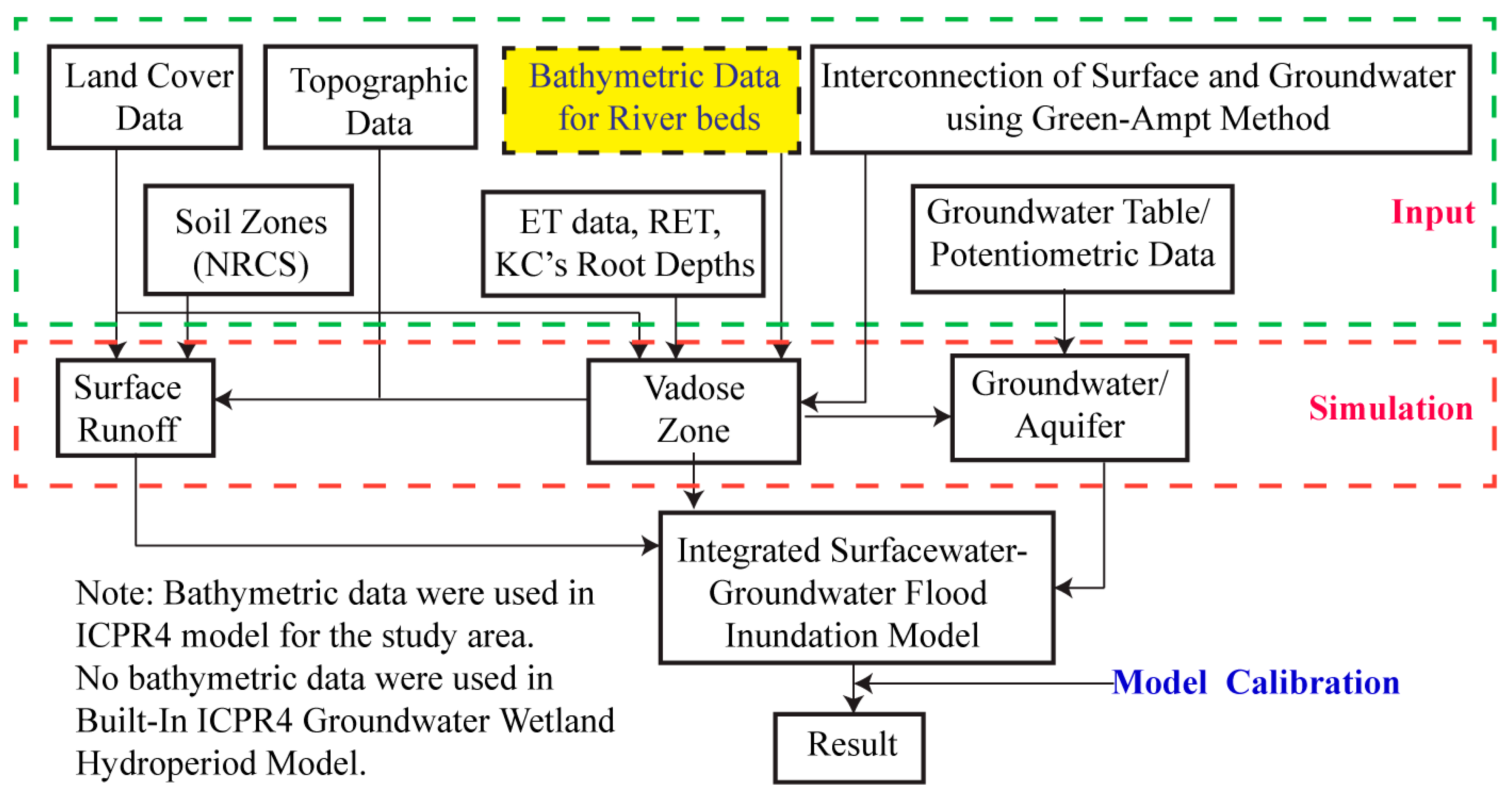
Figure 3.
Study area (Bear Creek Watershed) in Bay County, Florida.
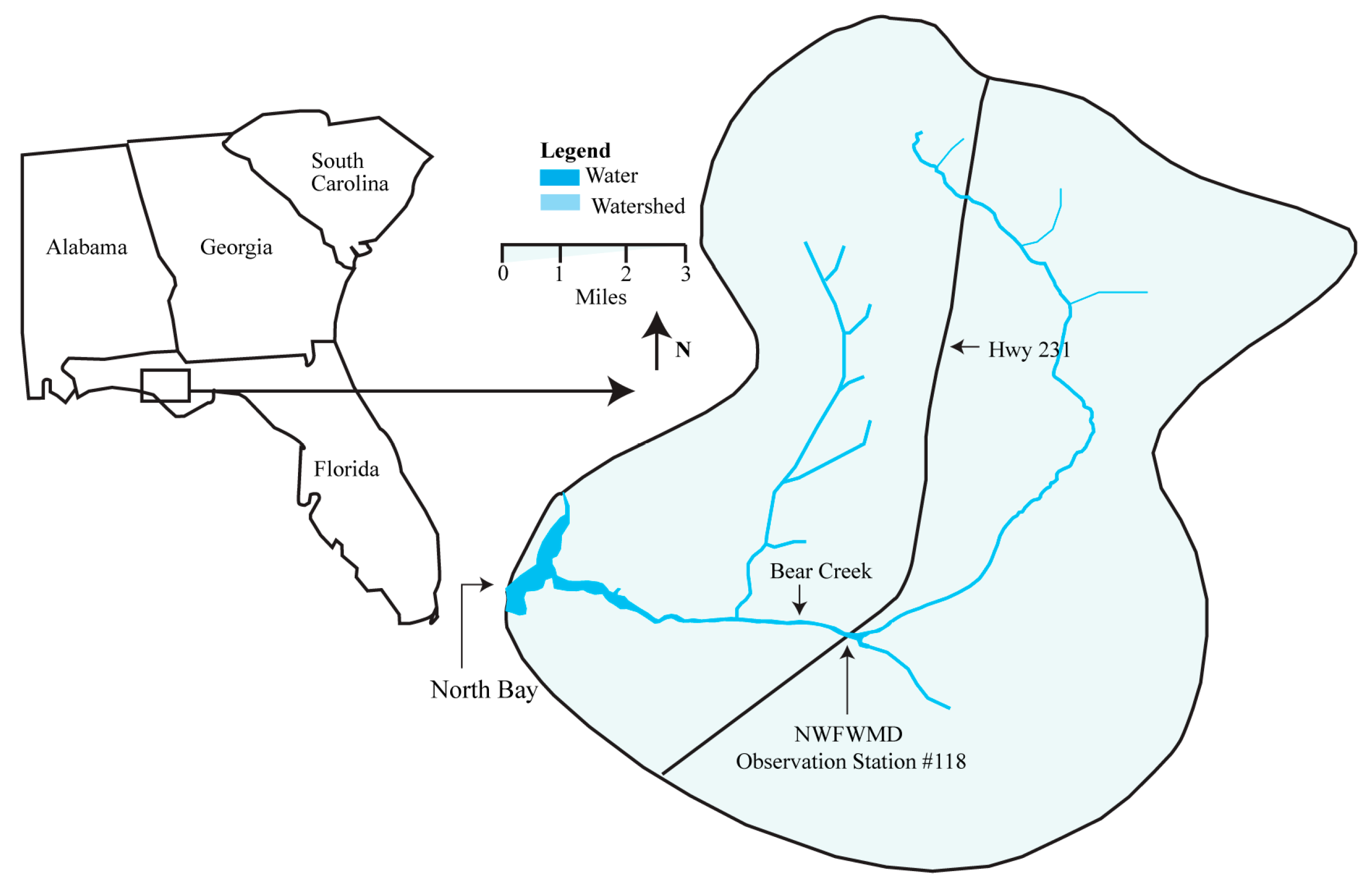
Figure 4.
Screenshots of maps and data of the Bear Creek Watershed at Bay County, Florida (used in the ICPR4 model). (a) Flow regions (Runoff region–red, Groundwater region– tan), (b) Topographic and Bathymetric Digital Elevation data, (c) Portal layout for the NRCS’s Web Soil Survey, (d) Green-Ampt Data Set, (e) Imperviousness Data Set, (f) Soil Zone map.
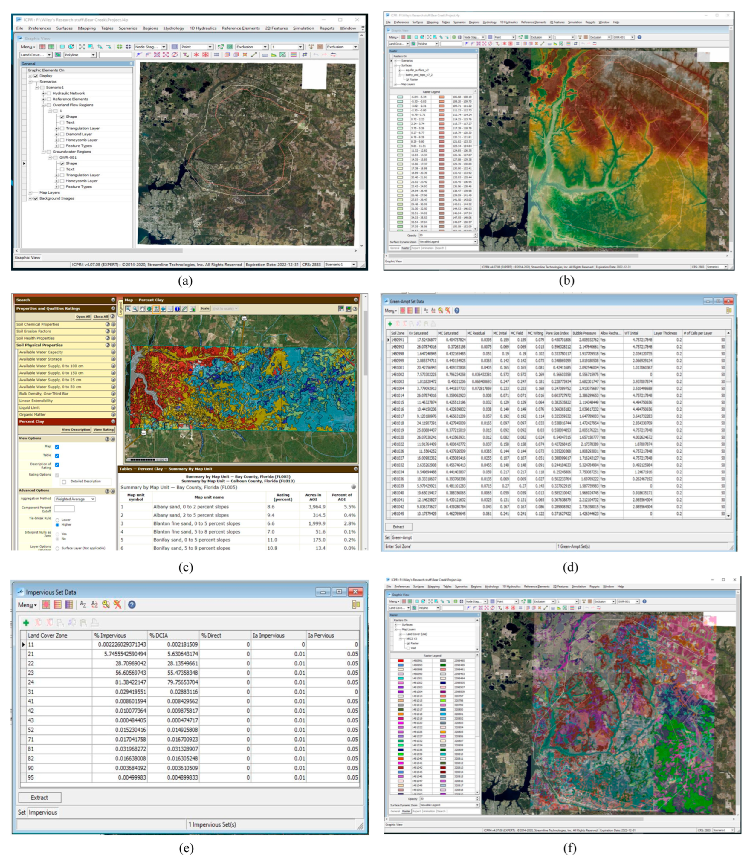
Figure 5.
Daily Precipitation From 2006 to 2023 with Trends (30-day Moving Average).
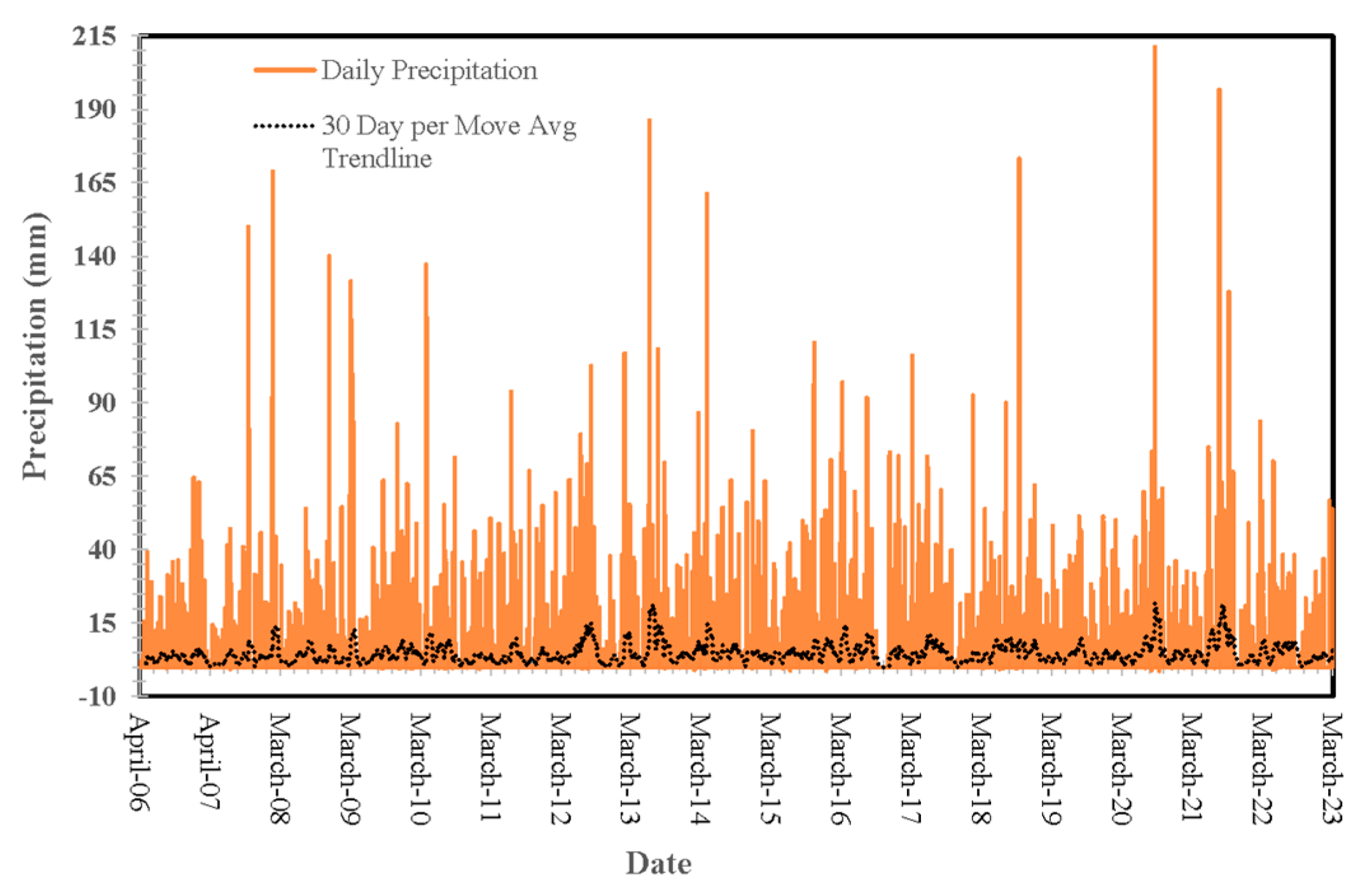
Figure 6.
(a) Annual Precipitation (1894-2022), (b) Annual Precipitation (1894-2010) and Annual Precipitation (2011-2012).
Figure 6.
(a) Annual Precipitation (1894-2022), (b) Annual Precipitation (1894-2010) and Annual Precipitation (2011-2012).
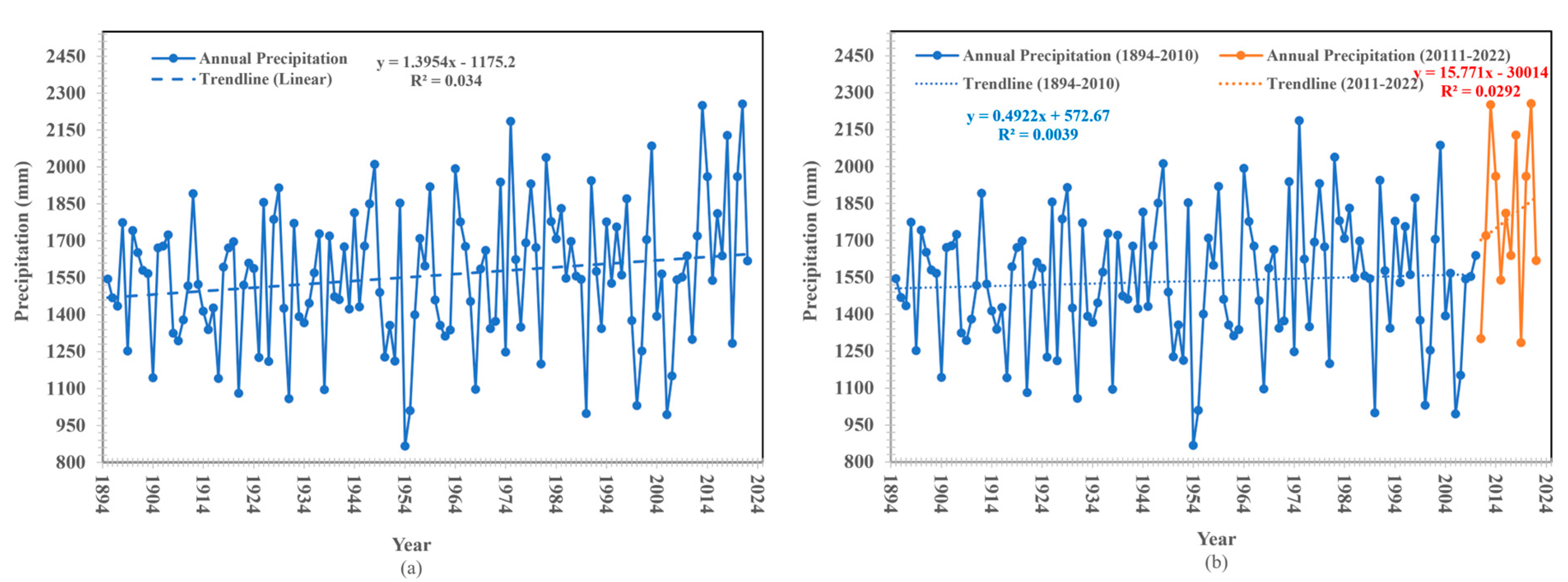
Figure 7.
Groundwater depth ( 2006-2023).
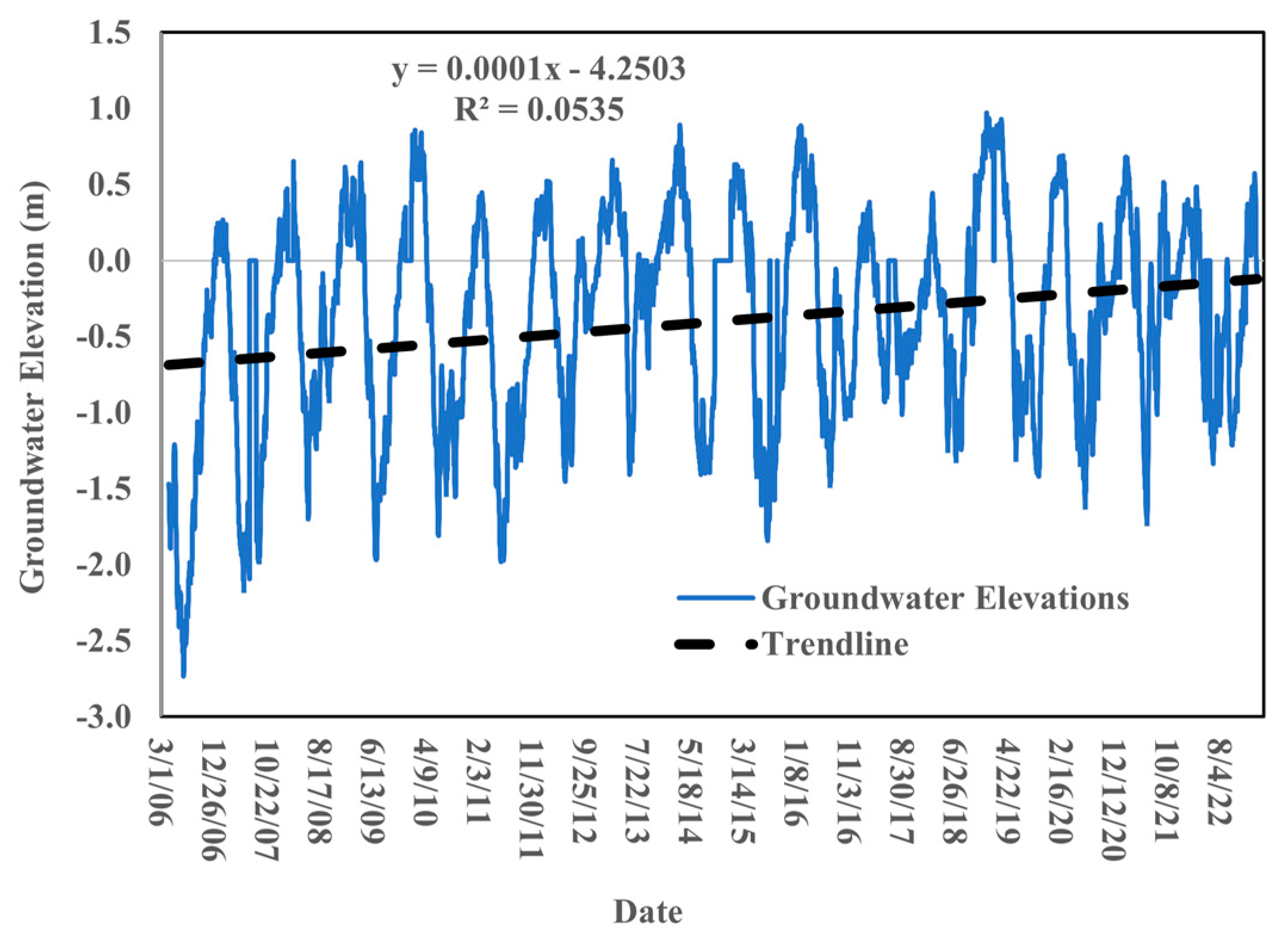
Figure 8.
Annual RET Trends From 1989 to 2018, Illustrating Long-Term Variations in Atmospheric Moisture Demand (1989-2018).
Figure 8.
Annual RET Trends From 1989 to 2018, Illustrating Long-Term Variations in Atmospheric Moisture Demand (1989-2018).
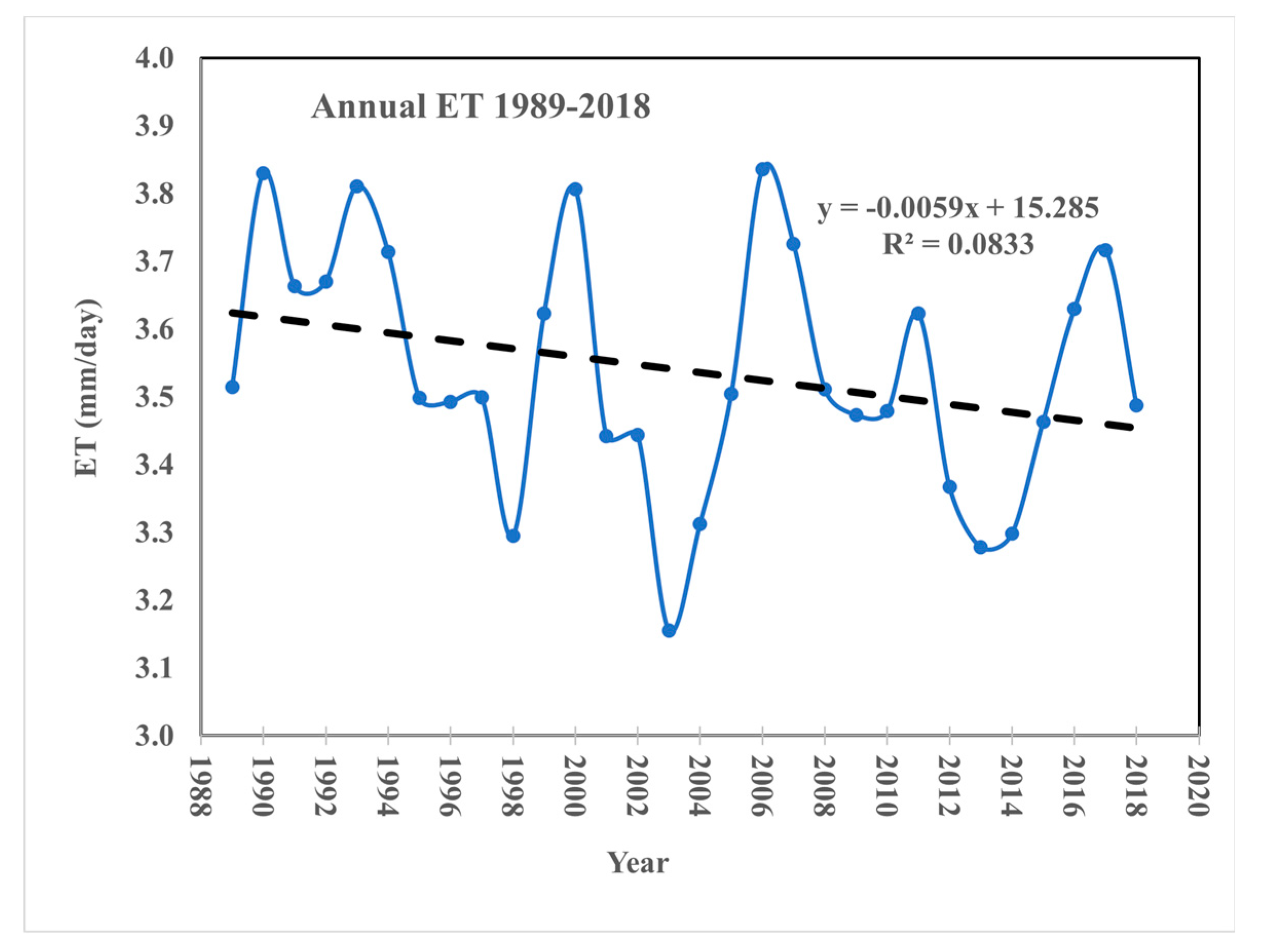
Figure 9.
Monthly Precipitation and Ground Water depth (2006-2023).
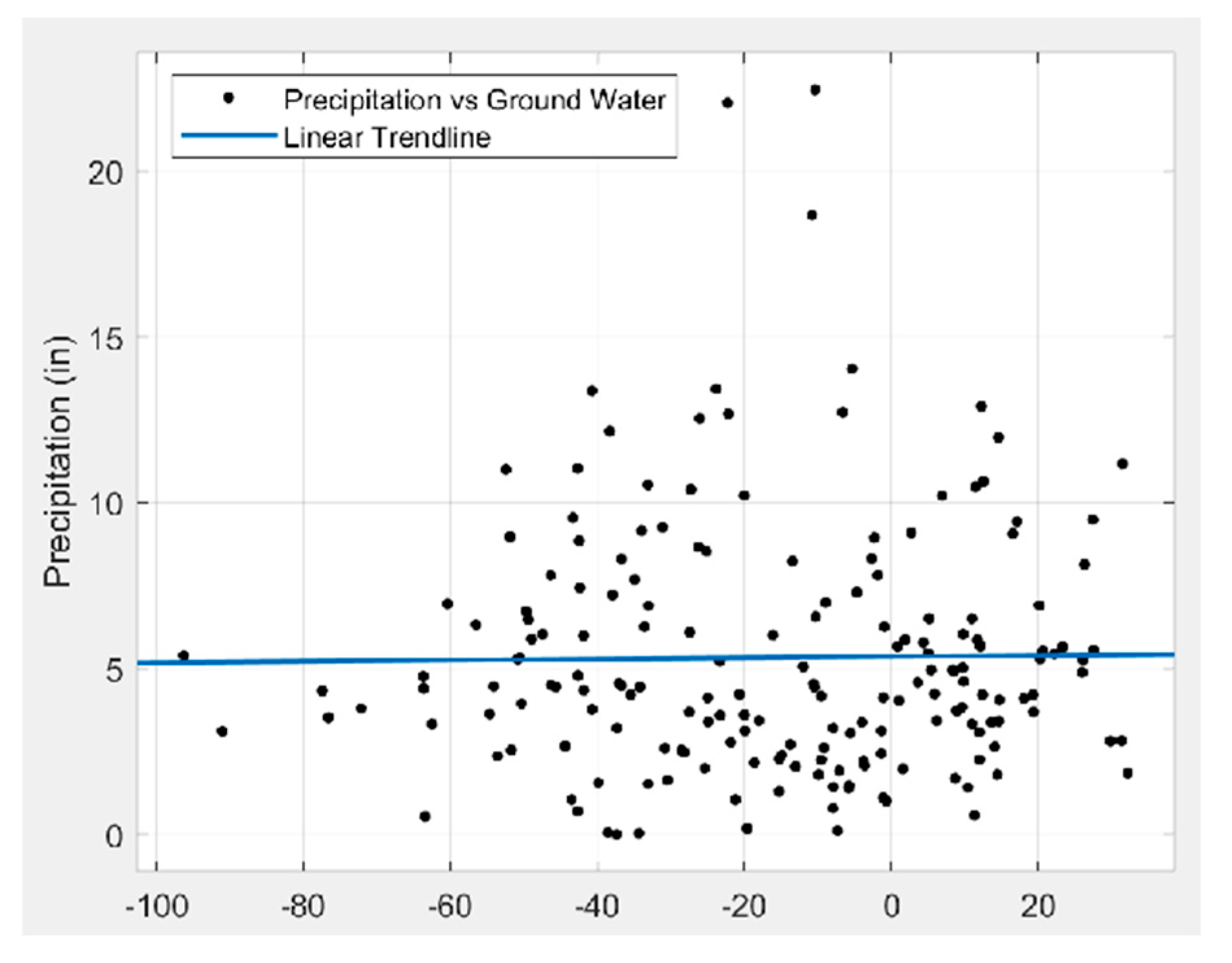
Figure 10.
Daily Ground Water Depth vs RET, 2011.
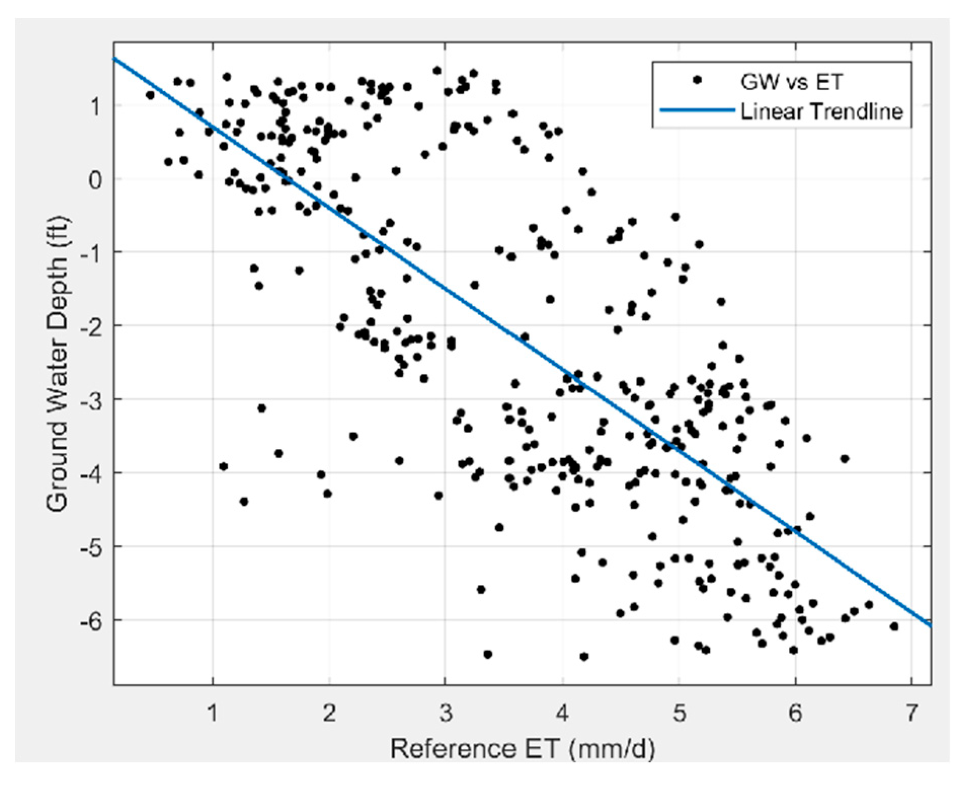
Figure 11.
Comparison of simulated groundwater depths (ft) under different ET conditions. (a) With ET, (b) Without ET, (c) animated color-scale legend.
Figure 11.
Comparison of simulated groundwater depths (ft) under different ET conditions. (a) With ET, (b) Without ET, (c) animated color-scale legend.
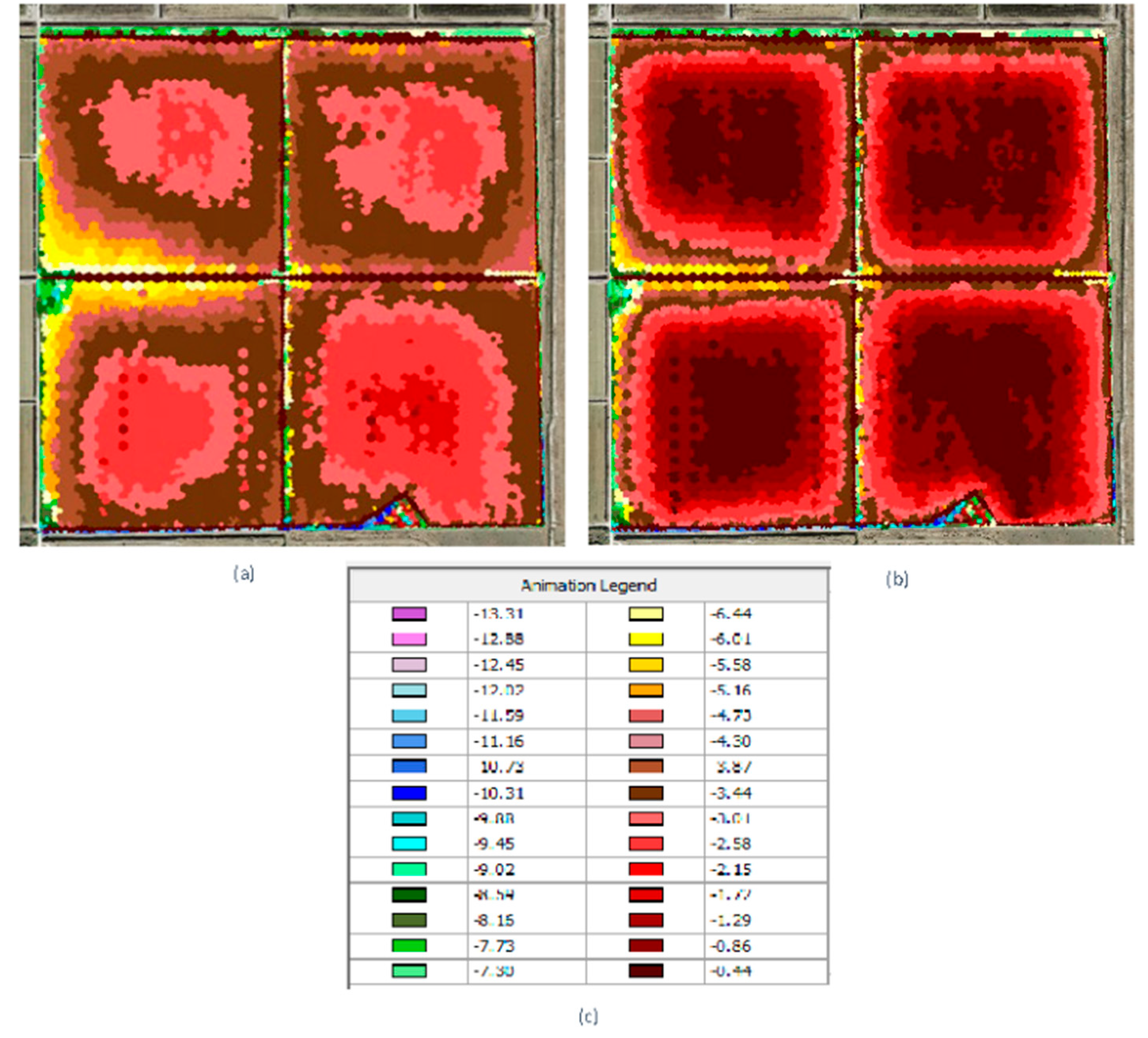
Figure 12.
Mass balance results for the example hydroperiod simulation. (a) With ET, (b) Without ET [2007,2008].
Figure 12.
Mass balance results for the example hydroperiod simulation. (a) With ET, (b) Without ET [2007,2008].
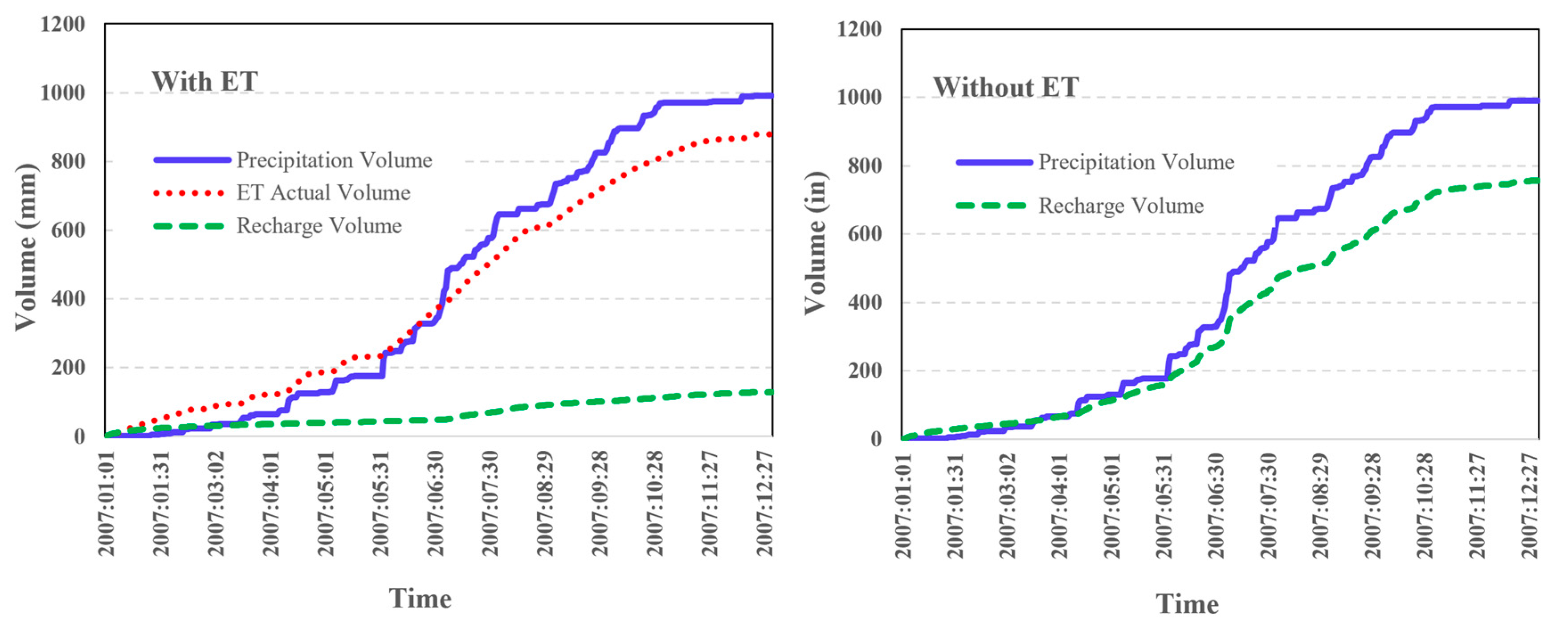
Figure 13.
Daily evapotranspiration and water-table elevation vs. time [2007,2008].
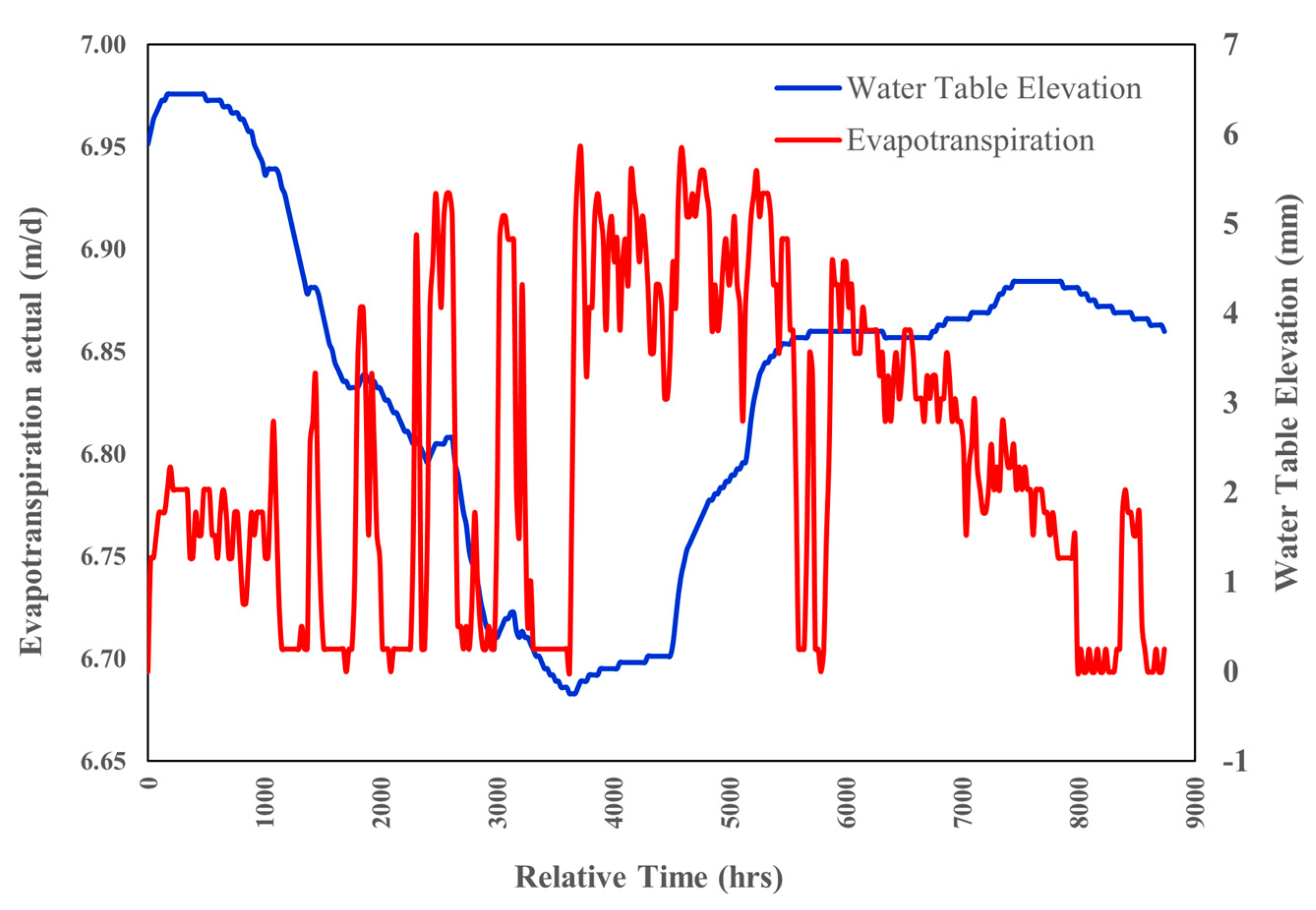
Figure 14.
(a) Simulation 1, 2016 MB Chart, with 2016 precipitation (b) Simulation 1, 2019a, MB Chart, with 2019 precipitation (c) Mass Balance Chart Legend.
Figure 14.
(a) Simulation 1, 2016 MB Chart, with 2016 precipitation (b) Simulation 1, 2019a, MB Chart, with 2019 precipitation (c) Mass Balance Chart Legend.
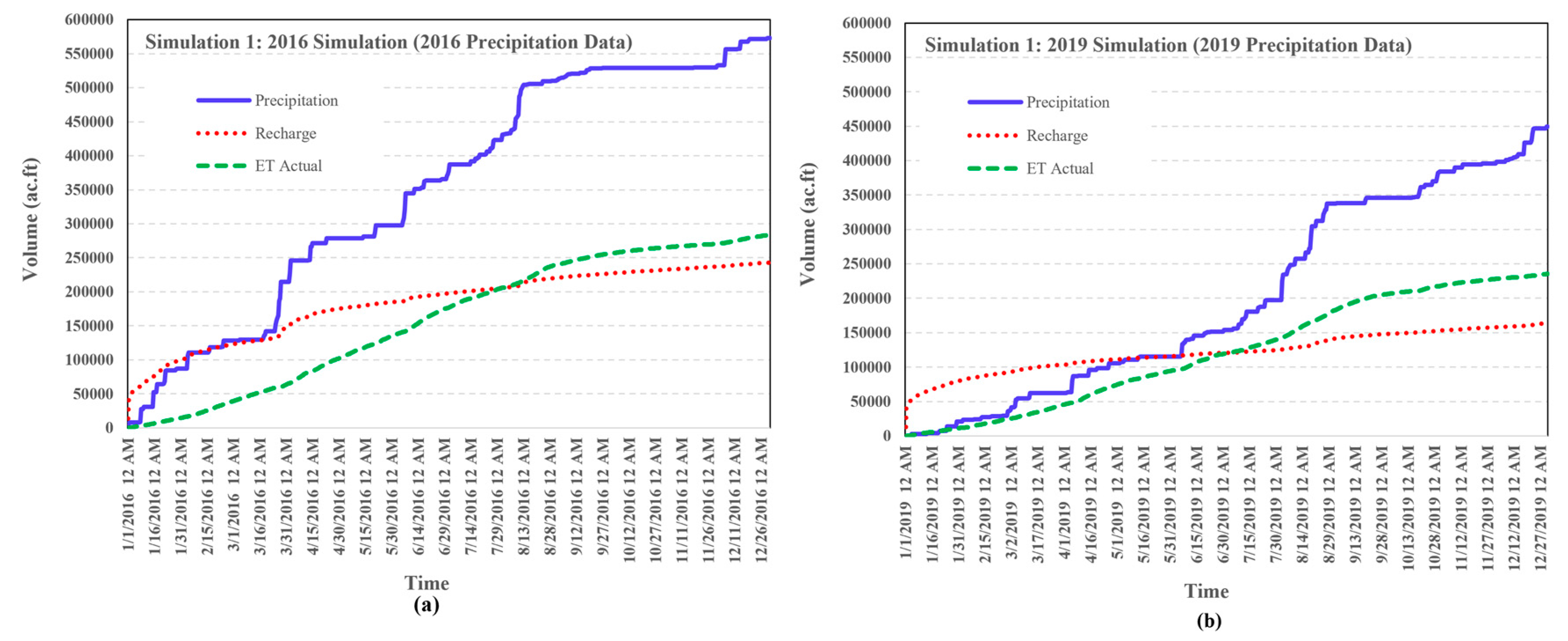
Figure 15.
Water Balance With 2016 Precipitation Data (a) 2016 Simulation (b) 2019 Simulation.
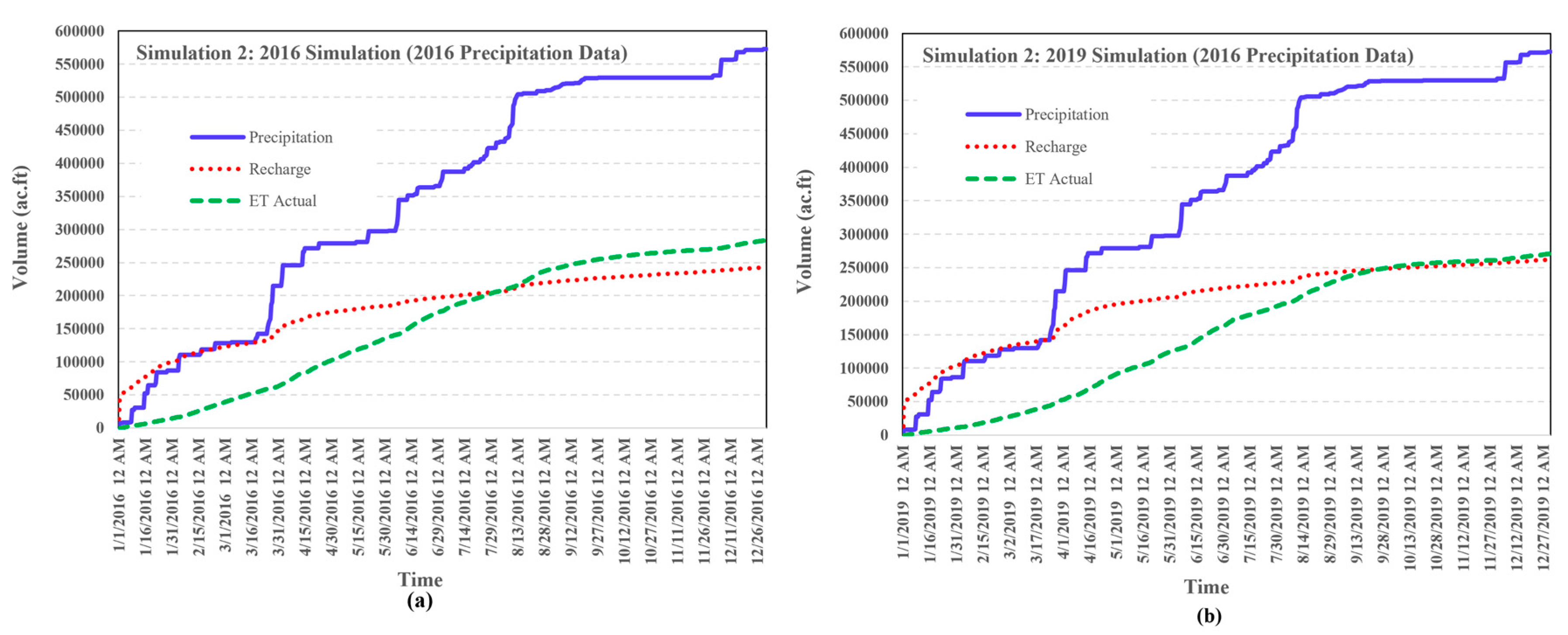
Figure 16.
Map of the Study Area Highlighting the Four Quadrants Where Stage Nodes Were Selected. (a) Locations of the Selected Stage Nodes. (b) Simulated Model Image.
Figure 16.
Map of the Study Area Highlighting the Four Quadrants Where Stage Nodes Were Selected. (a) Locations of the Selected Stage Nodes. (b) Simulated Model Image.
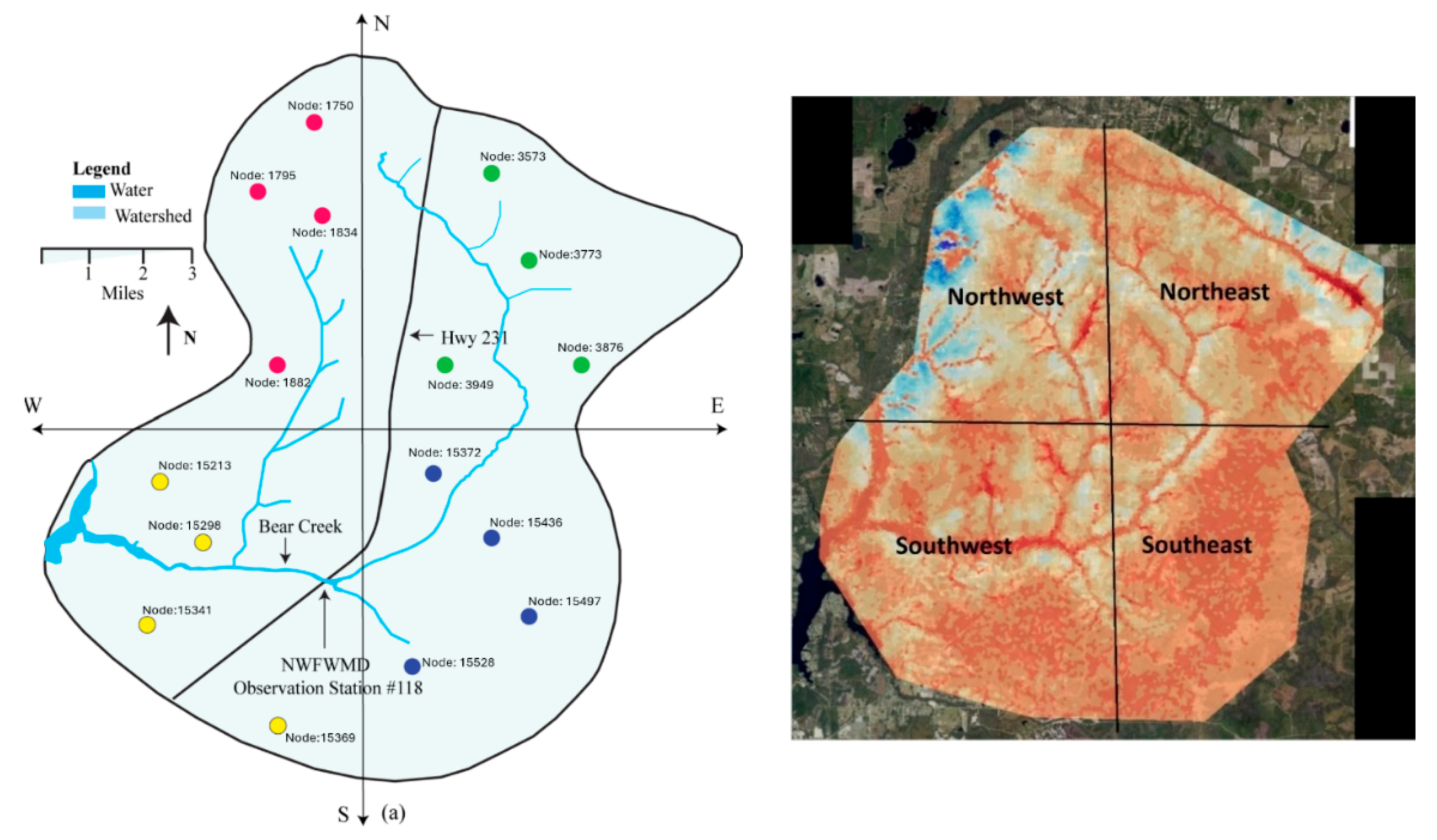
Figure 17.
Change in Groundwater Stages (Elevations). (a) Northeast Nodes, (b) Northwest Nodes, (c) Southwest Nodes, (d) Southeast Nodes.
Figure 17.
Change in Groundwater Stages (Elevations). (a) Northeast Nodes, (b) Northwest Nodes, (c) Southwest Nodes, (d) Southeast Nodes.
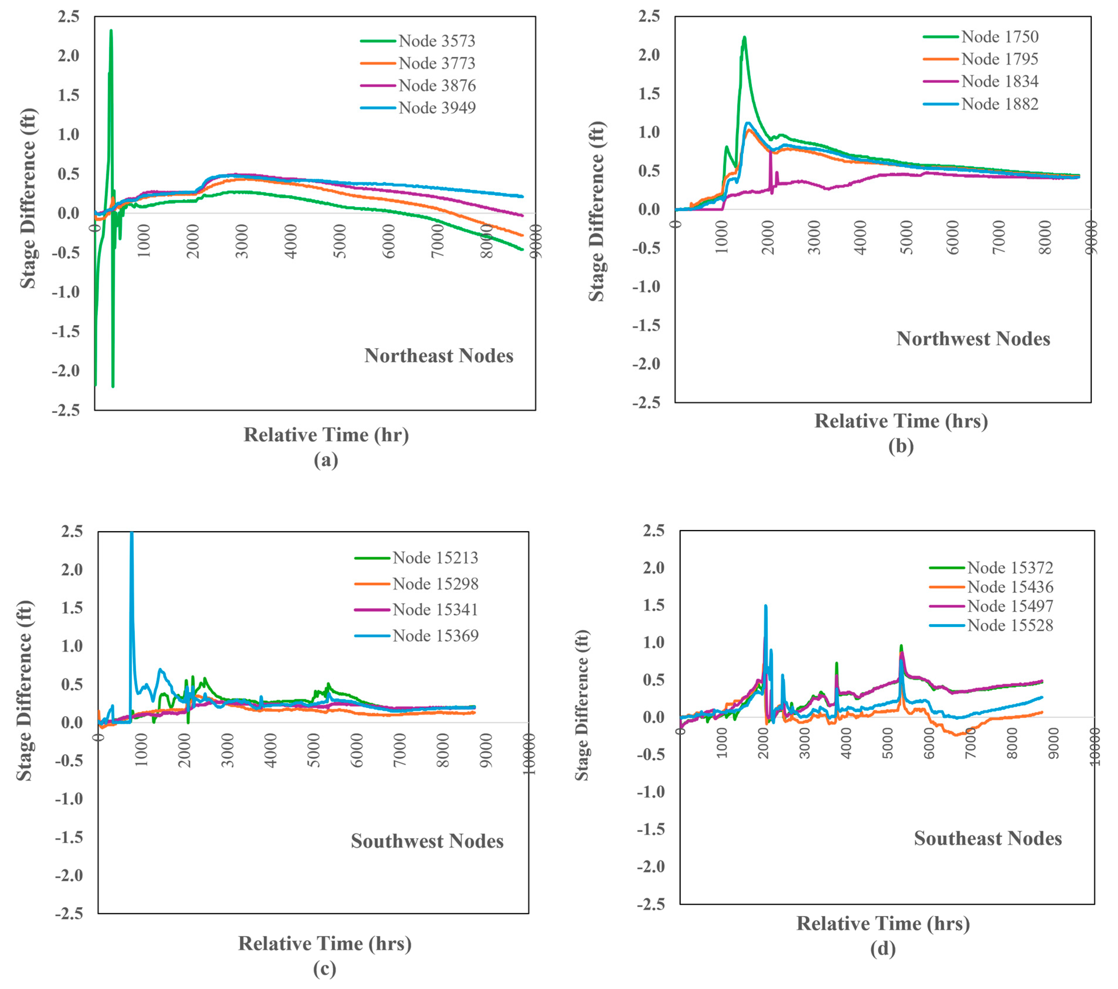

Table 1.
Land Cover Data for 2016 and 2019.
| Description | 2016 Area (ha) | 2019 Area (ha) | Change (ha) | Description | 2016 Area (ha) | 2019 Area (ha) | Change (ha) |
|---|---|---|---|---|---|---|---|
| Open Water | 253.9 | 198.2 | -55.7 | Mixed Forest | 2.0 | 31.0 | 29.0 |
| Dev, Open space | 2151.3 | 2099.7 | -51.6 | Shrub | 7033.9 | 8038.9 | 1005.0 |
| Dev, Low int | 837.9 | 849.4 | 11.5 | Grassland | 5408.1 | 6234.7 | 826.6 |
| Dev, Med int | 153.7 | 196.3 | 42.6 | Pasture/Hay | 362.0 | 359.4 | -2.5 |
| Dev, High int | 14.0 | 19.3 | 5.3 | Cultivated crop | 523.5 | 536.0 | 12.4 |
| Barren Land | 131.0 | 152.0 | 21.0 | Woody Wetlands | 13500.4 | 12872.7 | -627.7 |
| Deciduous Forest | 26.0 | 55.4 | 29.4 | Wetlands | 846.7 | 1516.8 | 670.0 |
| Evergreen Forest | 12476.8 | 10562.0 | -1914.9 | ||||
| Total area= 43,721 ha (169 mi2) | |||||||
Table 2.
Land Cover, Reference Crop, and Initial and Calculated Crop Coefficients.
| Land Cover |
Reference Crop | Initial Crop coefficient (Kc ini, Kc mid, Kc end) | Calculated Crop Coefficient | Plant Height (m) |
| Open Water | sub humid climate | 1.05 | 1.05 | - |
| Dev. Open Space | * Grass | 1 | 1 | - |
| Dev. Low Intensity | * Grass | 0.8 | 0.8 | - |
| Dev. Med. Intensity | * Grass | 0.5 | 0.5 | - |
| Dev. High Intensity | * Grass | 0.2 | 0.2 | - |
| Barren Land | * Grass | 0.15 | 0.15 | - |
| Deciduous Forest | Walnut Orchard | 0.5, 1.1, 0.65 | 0.5 | 18.28 |
| Evergreen Forest | Conifer Trees | 1 | 0.928 | 30.48 |
| Mixed Forest | Walnut and Conifer | 0.75, 1.05, 0.825 | 0.75, 0.983, 0.758 | 24.38 |
| Shrub | Berry Bushes | .3,1.05,.5 | .3,1.01,0.458 | 4.5 |
| Grassland | * Grass | 1 | 1 | - |
| Pasture/Hay | Bermuda Hay (average cutting effects) | .55,1,.85 | .55.981,.831 | 0.35 |
| Cultivated Crop | Conifer Trees | 1 | 0.928 | 30.48 |
| Woody Wetlands | Short Veg (no frost) | 1.05,1.10,1.10 | 1.05,1.056,1.056 | 6 |
| Wetlands | Reed Swamp (standing water) | 1,1.20,1 | 1,1.167,.967 | 2.4 |
Table 3.
Summary of ICPR4 Simulation Results (U.S. Customary and SI Units).
| Simulation | Scenario | Precipitation (in /mm) | ET (ac-ft/ha-m) | Recharge (ac-ft) | % Change in ET vs. 2016 | % Change in Recharge vs. 2016 | Main Observations |
|---|---|---|---|---|---|---|---|
| Sim-1 | 2016 | 63.44 / 1,611 |
283,814/ 35,008 | 243,100/ 29,986 | - | - | Higher rainfall led to high ET and recharge. |
| Sim-1 | 2019 | 49.9 / 1,267 | 235,552/ 29,055 | 164,247/ 20,260 | ↓ 17% | ↓ 32% | Lower rainfall reduced both ET and recharge; ET decrease did not increase recharge due to precipitation shortfall. |
| Sim-2 | 2016 | 63.44 / 1,611 | 283,814/ 35,008 | 243,100/ 29,986 | - | - | Baseline year with high vegetation. |
| Sim-2 | 2019b | 63.44 / 1,611 | 271,026/ 33,431 | 262,174/ 32,339 | ↓ 4.5% | ↑ 7.8% | Same rainfall as 2016; vegetation loss reduced ET and increased recharge, supporting hypothesis. |
Disclaimer/Publisher’s Note: The statements, opinions and data contained in all publications are solely those of the individual author(s) and contributor(s) and not of MDPI and/or the editor(s). MDPI and/or the editor(s) disclaim responsibility for any injury to people or property resulting from any ideas, methods, instructions or products referred to in the content. |
© 2026 by the authors. Licensee MDPI, Basel, Switzerland. This article is an open access article distributed under the terms and conditions of the Creative Commons Attribution (CC BY) license (http://creativecommons.org/licenses/by/4.0/).
Copyright: This open access article is published under a Creative Commons CC BY 4.0 license, which permit the free download, distribution, and reuse, provided that the author and preprint are cited in any reuse.


