
Submitted:
29 September 2025
Posted:
07 October 2025
You are already at the latest version
Abstract
The Breede Gouritz Water Management Area is critical for the agricultural and forestry industries, tourism, and property development. It is imperative to understand climate and related variable trends, groundwater depth and land cover trends, especially the interworking of these variables, which was the aim of this study. The catchment was divided into different climate and land cover subregions. A change detection analysis was utilized for four selected subregions, and the best models, according to the evaluation metrics, were used to forecast each variable into the near future. Relationships between variables were statistically correlated and compared to land cover trends. Results show that more arid/semi-arid areas expect temperature increases, evapotranspiration decreases, and precipitation decreases, rendering groundwater resources vulnerable. The temperate subregions to the West show mixed temperature trends and no trends in precipitation. Evapotranspiration is expected to increase. A rise in groundwater depth is expected in the near future, where increased precipitation is also expected. The impact of development in the entire subregion is already visible, with the possibility that urbanization and agricultural expansion could lead to diminishing wetlands and forests. Careful planning and consideration regarding groundwater resource management must be made, especially for vulnerable areas north and Northeast of the study area.
Keywords:
groundwater
; climate change
; land cover change
; statistical models
; change detection analysis
; forecasting
; correlations
; Breede-Gouritz
; South Africa
1. Introduction
Climate and land cover change (CLCC) have been influencing our hydrologic cycle since before its effects were discovered. Comprehensive studies on climate change (CC) in the context of water resources have been done, including groundwater resources, albeit to a lesser extent than surface waters. Land use and land cover (LULC) change is a relatively new area of research in the context of surface and groundwaters (Nkhonjera & Dinka, 2018; Hegerl et al., 2019) although its effects on water resources have been proven (Kundu et al., 2017; Wang et al., 2018). CC is influencing the hydrological cycle and, therefore, our water resources in the following ways: higher average worldwide temperatures, hot areas becoming even hotter and vice versa, wet areas becoming even wetter and vice versa, melting of glacial ice, sea-level rise and saltwater encroachment, changes in evapotranspiration rates, runoff rates, recharge and discharge rates, more intense storms, prolonged droughts and so forth (Jayakumar & Lee, 2017; Smyth et al., 2017). Ultimately, these perturbations influence our available freshwater supply. Dwindling freshwater supplies are under an even more significant threat due to the rising population and subsequent demand for water supplies (McCusker & Ramudzuli, 2007; Mogelgaard, 2012).
CC impact studies on water resources have been explored by many authors. For some time, global circulation models (GCMs) and regional circulation models (RCMs) have been downscaled and applied to more local scenarios (Kumar, 2012; Trzaska & Schnarr, 2014). However, it has been found that these results are not as accurate as when one uses field data such as historical climate records with an analysis on a regional-to-local scale. The climate is a regional phenomenon with local variations (McGregor, 2018; Wang et al., 2018). Historical data can aid in understanding precipitation, temperature and evapotranspiration trends, which can be applied to catchment scale scenarios. The latter is done to predict changes in streamflow, runoff, discharge, baseflow, recharge and ultimately water availability in future.
LULC impact studies have also increased (Correia et al., 2023). It is debated whether CC or LULC change significantly impacts our water resources (Andaryani et al., 2019; Olivares et al., 2019). Conclusions need to be drawn on a local scale. LULC change in the form of urbanization influences surface albedo, influencing evapotranspiration. Furthermore, urbanization affects runoff rates, consequently influencing recharge into groundwater stores. Deforestation and afforestation also influence water resources (Olivares et al., 2019; Berhail, 2019). Agricultural practices, whether croplands or pasturelands and the type of crops all have an impact on the circulation of water through the system and, ultimately, the freshwater supply (Fohrer et al., 2001; Hu et al., 2019; Touhidul-Mustafa et al., 2019). These variations are site-specific and must be accounted for appropriately in impact studies. Many LULC tools have been developed over the years, such as CLUE, DynaCLUE, and SWAT1 (Albhaisi et al., 2013; Shrestha et al., 2018; Adhikari et al., 2020). Moreover, calculations can be applied to LULC maps to determine the magnitude of the change and make future predictions.
The Breede Gouritz Water Management Area (BGWMA) is essential in South Africa as it is an area with vast agricultural activity, numerous export trades of agricultural stock, a robust tourism industry, property development and a supplier of fresh water to the City of Cape Town, which is strategically and economically important to South Africa. The City of Cape Town almost ran out of water entirely during a drought in South Africa between 2015 and 2017. Many research endeavours have been undertaken in the catchment, including a status quo report on all available surface and groundwater resources. Whilst it is critical to be proactive concerning the available groundwater resources and plan for the needs of future generations, no study has determined the future of groundwater resources in the area under current CLCC projections.
This study, therefore, presents a new analysis with advanced knowledge of CLCC trends over the past few decades. The first objective is to determine any underlying trends over the years via a change detection analysis. Secondly, statistical climate and groundwater depth projections will be made to determine the magnitude of anticipated trends in the near future. Lastly, a relationship between the climate and climate-related variables will be established by statistical means, and empirical relationships will be established between the former variables and land cover change.
2. Study Area Description
The selected study area is the Breede-Gouritz Water Management Area (BGWMA), governed by the Breede-Gouritz Catchment Management Agency (BGCMA). The boundaries are the Indian Ocean to the South, the Berg-Olifants Water Management Area (WMA) to the West, the Orange WMA to the North and the Mzimvubu-Tsitsikama WMA to the east (Figure 1). This WMA is mainly in the Western Cape, with overlaps in the Eastern and Northern Cape. It covers an area of about 72,000 km2, and has multiple land uses (Figure 2). The protection, conservation, management and control of water resources in the catchment are mandated by the BGCMA. The BGWMA provides an exciting platform to assess CC and LC impacts.
Generally, river water quality and conditions are good, but there is a call to use water more sustainably. There are 717 dams recorded in the water management area, ranging from very small to large. However, only 27 dams hold at least 5 million m3 of water. Managing groundwater resources is challenging because there is not a lot of data available. There are boreholes in the area from which data can be extracted (for example, water level, quality and geology logs), which will help to assess each aquifer. These boreholes are, however, mostly privately owned, from which data are rarely reported to the Department of Water and Sanitation (DWS). Another reason groundwater management is problematic is the underlying geology’s complexity and resulting water flow paths. The surface geology is inconclusive regarding the underlying geology and aquifer type and needs further investigation.
Precipitation enormously affects groundwater recharge and groundwater storage. It is imperative to determine water levels to see if abstraction rates are responsible and sustainable (Department of Water and Sanitation, 2017). More local and site-specific information is necessary to make proper conclusions about the groundwater situation in the BGWMA.
3. Materials and Methods
3.1. Data Sources
3.1.1. Climate Data
Climate data, temperature (T) and precipitation (P), in particular, were obtained from two sources: the Agricultural Research Council (ARC) and the South African Weather Service (SAWS). T was measured in degrees Celsius (°C), and the monthly average of the maximum and minimum daily average was used. P was evaluated by the sum of the monthly precipitation in mm. The ARC provided information from 11 stations scattered across the BGWMA dating back to 1924. The SAWS provided information from 25 stations scattered across the BGWMA dating back to 1990. Both sources reported maximum and minimum T and P data observed on a daily time step. Linear interpolation was used to calculate missing T values. In contrast, in the case of P, cross-correlations with neighbouring stations between the ARC and SAWS datasets were calculated, whereafter, the regression equation was applied between the two datasets to fill in missing values. Only one station in each selected subregion was chosen for further analysis. Figure 3 displays the geographic distribution of the selected ARC and SAWS stations.
3.1.2. Actual Evapotranspiration
Actual evapotranspiration (ET) maps that were recorded on a monthly timescale (in mm) have been obtained from the WaPOR site. These maps date back from January 2009 to the present. The data are in raster format with a resolution of 250 m. Monthly totals were obtained by estimating ET in mm/day, multiplying it by the number of days in a dekad (ten days), and then using each month’s average. Relevant data were extracted per Köppen-Geiger climate subregion, 8 in total. The extracted pixel values were multiplied by a factor of 0.1 and used as a variable in a time-series analysis. No data pixel values were omitted. Moreover, individual shapefiles were created for the four selected subregions (BWh, BWk, Csb and Csa) to compare each LC class’s area change per subregion between 1990, 2013/14 and 2020.
3.1.3. Groundwater Data
Groundwater data from the Breede and Gouritz Catchments have been obtained from the National Groundwater Archives (NGA) and the Hydstra database from the DWS. All borehole recordings recorded static water levels. In some cases, an autographic recorder was used to record data in many boreholes, meaning multiple daily measurements could be made. However, for most boreholes, monthly observations were recorded. A dip meter was used for older recordings. After filtering the NGA data, only 35 boreholes from the Breede Catchment and 130 from the Gouritz Catchment had data recorded for at least ten years. From this dataset, reference boreholes (8 in total) were selected for each climate subregion where available, and a change detection analysis was run for each borehole. After filtering the Hydstra dataset, only 14 boreholes were selected for further analysis (Figure 3 and Table 1)
The selected boreholes were chosen based on specific criteria, which include proximity to a chosen weather station, preferably in the same quaternary catchment and on the same side of a watershed (at least the latter if the former is not possible), and the number of consistent data points available (at least ten years). For each location, boreholes were statistically correlated (section 4.1), and the resulting boreholes with the most significant correlations were chosen for time series analysis. Monthly averages were used for groundwater depth. Where there was missing information, linear interpolation was used to fill in missing gaps, assuming no significant change occurred between the previous and the subsequent measurement. Every effort has been made to choose appropriate boreholes with significant data and minimal missing values. However, only a few were deemed appropriate.
Groundwater depth (GWD) was analysed in this study (in metres); however, a few assumptions about the observed GWD were made during the analysis phase of this study. The first assumption is that GWD’s seasonal patterns indicated recharge patterns and were closely compared to P in each subregion. Secondly, it is assumed that the observed GWD is due to CC, mainly P since no abstraction data are available. Lastly, suppose GWD rises, in other words, the point at which water is first encountered is closer to the surface than expected. In that case, it is assumed that the respective aquifer has experienced recharge and a resultant increase in storage.
3.1.4. Land Cover Data
National land cover (NLC) maps determined the change in land cover (LC) between 1990 and 2020. These maps were generated using Multispectral Landsat 4/5 imagery at a 30 m resolution for the 1990 and 2013/14 maps. The 2020 map is an updated version of the 2018 map and was mapped with a 20 m resolution from Sentinel 2 imagery. The 1990 and 2013/14 maps had 72 classes, whereas the 2020 map had 73 LC classes. For this study, those classes were grouped into ten categories. These categories highlight significant LC classes while simplifying the comparison and analysing LC change (Figure 2).
3.2.1. Delineation of Climate and Land Cover Subregions
The BGWMA was divided into different climate subregions based on the Köppen-Geiger climate classification (Beck et al., 2020) (Figure 3) and into different LC subregions using the latest NLC map (Figure 2). Only four subregions were chosen for discussion: BWh, BWk, Csb and Csa. These subregions were chosen because they had significant available data for analysis from which firm conclusions could be drawn. Sufficient GWD data were also available in these subregions, which could be analysed individually and correlated with other variables. Lastly, ET patterns in these subregions and strong relationships between ET and variables other than T were also considered in this selection. The boreholes analysed for the BWh subregion are technically outside the quaternary catchment and climate subregion but are on the same side of the watershed, downstream of the Gamka River. It was the only available data.
3.2.2. Change Detection Analysis: Magnitude of the Impact of Temperature, Precipitation, Evapotranspiration, and Groundwater Depth
A change detection analysis was performed using Python software for T, P, ET and GWD from selected weather stations (variables T and P), boreholes (variable GWD) and climate subregions (variable ET). This change detection analysis determined existing data trends and was used to make near-future forecasts. The models were trained on 70% of the dataset, from which a validation forecast was made and compared to the actual values of the remaining 30% of the data using four evaluation metrics: mean squared error (MSE), root mean squared error (RMSE), mean absolute error (MAE) and mean absolute percentage error (MAPE). The model with the best evaluation metrics was chosen to forecast the near future. To verify the models, they were compared with decomposition plots that distinguish between a dataset’s trend, seasonality and residual noise. Furthermore, the Mann-Kendall (MK) test is a non-parametric test used to verify observed trends in the data. In summary, for each variable, the following processes and methods were employed in this order (Figure 4):
4. Results
Climate and climate-related results (T, P, ET, GWD variables) are reported per climate subregion. LC is discussed in section 4.2. T and P trends are related to the weather station in question but representative of the subregion. GWD trends are related to the closest weather station. ET trends are spatial.
4.1. Climate and Climate-Related Trends Per Subregion
4.1.1. BWh
The BWh subregion covers 8,16% of the study area and is characterised by an arid, desert environment and hot conditions (Figure 3). The Mean Annual Temperature (MAT) is 18.6 °C and the Mean Annual Precipitation (MAP) is less than 256 mm a year. The average annual P between 2014 and 2020 was 121 mm. The LC of most of this subregion is bare land, and much less so is some grassland areas. The boreholes are situated in a valley adjacent to the Swartberg Pass, at a higher elevation than the station, and towards the South of the weather station. The aquifer is fractured with a minimal yield.
T, P, ET and Hydstra GWD data are available for this subregion. T, ET and GW data are not stationary and indicate a trend. Boreholes J2N0580 and J2N0621 indicate a difference stationarity. According to the decomposition plots (Figure 5), a slightly positive trend for average monthly T between 18 °C and 20 °C is evident, and a simple, expected annual seasonality with hot summers and cold winters is observed. A decreasing P trend is observed between 20 mm and 15 mm monthly summative precipitation. P is higher at the beginning of the year, consistent with late summer P patterns over South Africa (Kruger, 2007), after which it declines in an oscillating fashion. The ET trend is typically higher at the beginning of the year. GWD increases early in the year (February/March), peaks midway through the year and declines sharply until the end of the year or early in the following year. For some boreholes, the recharge is faster than for others, such as J2N0620. The recharge observations indicate the reliance on P as the recharge patterns follow the P season, albeit at different rates in respective boreholes.
Correlations between variables are generally not very strong (Table 2); virtually no relationship exists between T and P; however, a significantly strong positive relationship exists between T and ET. ET and J2N0582 have a slight positive relationship with P. All the boreholes are correlated, some more pronounced than others, for example, J2N0580 and J2N0582 with borehole J2N0621. J2N0621 is also firmly positively correlated with ET. For the most part, Spearman’s rank indicates slightly stronger relationships, especially among the boreholes and T and ET. Pearson displays a more robust relationship (albeit still weak) between P and ET and ET and J2N0621. These positive correlations illustrate that one variable is likely to increase with the other one or vice versa (Pearson’s), albeit monotonic or not at a constant rate (Spearman’s).
The MK test confirms the decreasing trends observed in P and ET, respectively (Table 3). T displays an increasing trend. All of the boreholes’ GWDs show decreasing trends. An increase in T from 19.5 °C to 20.5°C between 2021 and 2028 is forecasted (Figure 6a). Moreover, a decrease in P from 6 mm to 0 mm monthly totals is expected between 2021 and 2028. ET indicates a decreasing forecast from 32 mm to 20 mm between 2022 and 2036. Borehole J2N0580 is expected to decrease from -18 m to -30 m, whereas borehole J2N0582’s future forecast is at a lower constant than the validation forecast, from -12.5 m to -13.75 meters. J2N0620 show a decrease from -11.25 m and -14.25 m. J2N0621 show a new constant of -14.25 m for the future phase, 4 meters below -10.25 m, the constant for the validation phase (Figure 6b). An increase in T is highly likely in this subregion, which means that if P increases, ET should increase. In the latter case, GWD in specific boreholes could, therefore, potentially also rise. However, a decrease in P is expected, which would negatively impact ET and GWD recharge.
4.1.2. BWk
The BWk subregion, as the second largest subregion, makes up 30.53% of this study area (Figure 3). Cold, aridic desert-like conditions characterise this subregion. The MAT is lower than 18 °C and the MAP is a function of the MAT depending on the precipitation season; in this summer precipitation area, the MAP is less than ten times the MAT plus 28. The MAP for Beaufort West between 1994 and 2020 was 258.6 mm. The LC consists primarily of bare land, shrubland, and a few areas that overlap with grassland areas and irrigated agriculture. The boreholes are all in the same quaternary catchment as the weather station and on the same side of the watershed. The Hydstra boreholes are in sporadic locations, including in the valley and cut out by the Gamka River to the North (J2N0001). Various fractured aquifers in this area have differing yields.
Good quality T and P data observed on a daily time-step for over 20 years with minimal missing values are available for this subregion. The same holds for ET data, but data have only been available since 2009. Good quality GWD data from the NGA and Hydstra datasets has been observed for multiple boreholes in the Beaufort West region. Beaufort West was analysed for all four variables and was used as the example modelling station. Beaufort West T, ET and GWD data for nine of the ten boreholes are not stationary. T, ET and four boreholes display trend stationarity.
According to the decomposition plots (Figure 7), Beaufort West indicates a gradual increase in T from 17 °C to 19.5 °C. An annual T seasonality, higher Ts in the summer and low Ts in the winter is observed. P varies between 20 mm and 55 mm over the entire period. It displays a robust seasonal component with relatively higher P in the summer months (December to February), followed by a sharp decrease and an oscillating climb from May/June until December again. ET is displaying an overall decreasing trend, with a similar seasonality observed before; a steady climb into the summer months, oscillating behaviour until March and then a decline until mid-year. NGA boreholes show a similar seasonal pattern. The year starts, and the GWD increases until February/March, after which it decreases until about August/September, although this pattern’s starting and ending times vary slightly in different boreholes.
Hydstra GWD datasets’ seasonality behaviours are similar, with an increase usually at the beginning of the year for a couple of months and then a decrease the rest of the year. J2N0001 has a simple seasonality with a sharp increase from December to mid-year, after which an immediate decrease for the rest of the season follows. J2N0043 display an increase from the end of the previous year, little variability for a couple of months and a sharp decrease for the rest of the season. The recharge lag time is relatively far behind the P peak, which could indicate a slow recharge. The GWD of 3222BC00179 is expected to rise and is situated 4.71 km Southwest and at a lower elevation than the station. H2N0041 and J2N0043 are 10.1 km N and 9.1 Northnorthwest from the station, respectively, in the valley at a higher elevation. This could indicate that the boreholes’ recharge lag time in the valley is longer.
A robust positive relationship between T and ET and a weak correlation between T and P (Table 4 and 5) is evident. The correlation between T and ET is the same as Pearson’s and Spearman’s, indicating a linear yet monotonic relationship. Pearson’s rank shows a more robust relationship between T and P and P and ET, which indicates a linear positive relationship (Table 5); P and ET are associated with warmer weather. All the boreholes display strong correlations except correlations with 3222BC00152 and 3222BC00179, although the latter correlation is still significant. A relatively significant negative relationship exists between T and 3222BC00152 and J2N0019, respectively. Spearman’s correlations are stronger among the Hydstra boreholes, whereas between the NGA boreholes, the correlations are more linear except for 3222BC00152. The MK test (Table 6) shows an increasing trend in T and borehole 3222BC00179 and a decrease in P, ET and all Hydstra boreholes.
The statistical models that proved the most suited include linear regression for T, P, and ET (Figure 8a). GWD models are a mix of all four models. T is expected to increase slightly from 18.75 °C in 2021 to 19.5 °C in 2040. P is expected to decrease from 15 mm to 8 mm monthly summative P for the same period as the T. Between 2021 and 2036, ET is expected to decrease from 40 mm to 32 mm per month. GWD from ten boreholes were modelled respectively, of which five display no significant trend (3222BC00170, 3222BC00152, 3222BC00171, J2N0019 and J2N0550). 3222BC00179 shows a rising trend according to the linear regression model from -13 m to -7 m between 2006 and 2028. GWD for boreholes J2N0001, J2N00041, J2N0043 and J2N0618 is expected to decrease from -23 m to -43 m, -35 m and -53 m, -30 m and -50 m and -32 m and -41 m respectively between 2020/22 and 2036/40 (Figure 6b,c–d).
Given the results, an increase in T is highly likely in the near future of this subregion, which could drive the process of ET at a more robust rate, provided there is sufficient P. However, P is likely to decrease, which could negatively impact ET. GWD recharge time seems to follow P seasons; however, it is at a much longer lag than previously observed.
4.1.3. Csb
Towards the West is the Csb subregion, which covers an area of 10.57% of the BGWMA (Figure 3). It also has a temperate climate but with dry and warm summers. The P in the driest month of summer is less than 39 mm, and a third of the P in the wettest month is still more significant than in the driest summer month. The LC consists of vast areas of dryland agriculture, spots of irrigated agriculture (minority), shrubland, grassland, bare land, indigenous forests and urban areas, especially towards the coast. Large water bodies are also observed. The weather station and borehole 3419AD00004 are in the same quaternary catchment and on the same side of the watershed. The borehole is situated on a golf course about 0.5 km from the ocean at its closest point; however, it is no longer used and was a fractured aquifer.
Good quality T and P data have been recorded daily for over 20 years. GWD data are also scarce in this subregion; however, some data were available for Hermanus, but only between 1956 and 1984. Nonetheless, the data were used for analysis, and Hermanus was chosen as the model station for this region. All data were stationary except for ET and GWD, exhibiting trend stationarity. A typical T seasonality is observed for Hermanus (Figure 9). P seasonality is almost opposite that of T; low P in summer and high P in winter. The same seasonality pattern is evident for ET as was previously described. GWD seasonality is opposite to T: low in summer and high in winter. GWD seasonality follows P: low in summer and high in winter. Recharge is relatively rapid, consistent with the rainy season, which illustrates the importance of recharge in the area for GWD recharge.
Relatively strong negative relationships have been confirmed between T and P for Hermanus (Table 7). This relationship and the negative correlation between P and ET are more robust with Spearman’s rank, indicating a negative monotonic relationship; P is associated with colder T, and ET is more prominent in warmer Ts. A solid positive and more linear relationship between T and ET confirms the latter observation. A negative relationship is evident between P and ET. The MK test (Table 8) confirmed an increasing trend for T, P and ET and no trend for GWD. The linear regression forecasting model proved to be the best model for the Hermanus area (Figure 10a,b). Between 2021 and 2040, T displays an insignificant trend from 17.4 °C to 17.65 °C, and P is expected to increase from 42.5 mm to 48 mm. ET shows an increase between 2022 and 2036 from 63.4 to 64.5 mm per month at a constant rate. GWD indicates no significant trend.
If significantly elevated T levels should occur in the future, ET is highly likely to increase, provided sufficient P. Although no significant GWD trend is observed in this dataset, P perturbations are highly likely to influence GWD since recharge follows P seasonality.
4.1.4. Csa
This temperate subregion with dry and hot summers (Figure 3), Csa, is similar to the climate of Csb. The MAT is 18.7 °C and the P in the wettest month (June) is more than three times that of the P in the driest month. This winter P area receives a MAP of 272.31 mm (between 1999 and 2020). Csa subregion covers an area of 1.18%. The LC consists of shrubland, mostly irrigated agriculture, a large waterbody, some urban areas (Worcester) and a few relatively small areas of dryland agriculture. Three of the boreholes are in the same quaternary catchment (30959/H1N0018, H1N0055), and all of them are on the same side of the watershed at more or less the same elevation, between 204 and 209 m. 30959/H1N0018 are adjacent to the Breede River, next to the riverbed, between the Breede River and Brandvlei dam. 3319CB00003 is between two tributaries on bare land. H1N0055 is the closest to the weather station, just over a kilometre on a farm. H2N0521 in the industrial area. 3319CB00015 is on a farm near Breede River and is an intergranular aquifer of high yield. All other aquifers are fractured aquifers.
All four variables were analysed in this subregion, and good quality T, P, ET and GWD data were available. T, P data were available from 1997 to the present, ET data from 2009 to the present, and NGA GWD data between 1982 and 1992. Three Hydstra GWD datasets were available for analysis, of which H1N0018 is a continuation of 30,959 (data gap of 6 years between 1993 and 1999). Worcester was used as the modelling weather station. The data are stationary according to the ADF and KPSS tests, except for a trend component for T and ET. Hydstra datasets indicate difference stationarity.
According to the decomposition plots (Figure 11), no clear trends are seen for T and P, but ET shows an increasing trend. The T seasonality is the typical sine-like curve. In contrast, P seasonality is almost opposite to T, with low P in the summer months and relatively higher P in winter in the middle of the year. The increase in P is rapid just after the new year until about April, after which it declines at a gradual pace. However, with fewer variations, a similar seasonality pattern for ET is observed for the other subregions. GWD seasonality is essentially the same for all three boreholes; a rising pattern is observed until April, then lowering to July/August, and then slowly rising again. Hydstra datasets indicate that groundwater starts the year with a decline, reaches its lowest point in February/March, rapidly increases, varies at its peak and then declines in the second half of the year until just after the new year. GWD recharge following the winter P season is relatively slow. The recharge lag time for H1N0018 and H1N0055 is about 6 to 7 months after the rainy season, whereas the other boreholes, between 5 and 10 km from the station, all show a faster recharge time.
This study’s most robust negative relationship between T and P is seen here (Table 9 and Table 10). A significantly strong positive linear relationship between T and ET and a negative relationship between ET and P is observed. The relationships between T and P and P and ET are more strongly negative, with Spearman’s rank indicating a non-linear monotonic relationship. T has a slightly negative relationship with H1N0055, which is more robust with Spearman’s rank, i.e., not linear. P has a slight positive relationship with H1N0018 and H1N0055. H1N0018 and H1N0055 have a strong positive relationship. The other Hydstra GWD relationships are positive but not as robust as between H1N0018 and H1N0055. The NGA boreholes are all significantly positively correlated. Since all NGA boreholes are positively correlated and 30,959 is the old H1N0018, the assumption is that most boreholes, except for H2N0521, are positively correlated and follow similar patterns. Therefore, a slight positive relationship between P and borehole H1N0055 could mean P is influential in GWD recharge.
The MK test (Table 11) results reveal a decreasing trend for T and borehole H2N0521 and an increasing trend for ET and boreholes 30959, 3319CB00015 and 3319CB00003. The models that best fit the variables in this region are a mix of linear regression, Prophet and Auto ARIMA (Figure 12a–c). Between 2021 and 2040, this model indicates a significant negative trend in T from 19 °C to 18 °C. No trend for P is observed. ET, however, increases from 67 mm to 71.2 mm between 2022 and 2036. NGA boreholes 30959, 3319CB00015 and 3319CB00003 all display rising trends; however, the projections could only be made up until 2002 (from -2.4 m to -2.25 m, -1.75 m to -0.75 m, and -1.75 m to -1.48 m respectively). Hydstra boreholes H1N0018 and H1N0055 display no significant trends, whereas H2N0521 lowers from -0.04 m to -0.09 m between 2022 and 2040. T is expected to decrease in this area, and P is expected to increase, which could result in lower levels of ET. Furthermore, recharge could be P-dependent; therefore, the higher the P, the higher the resulting potential recharge, especially in the vicinity of borehole 3319CB00015.
4.2. Land Cover Trends
LC change was determined from the NLC maps for 1990, 2013/2014, and 2020. From 1990 to 2020, the study area observed an increase in urban, dryland and irrigated agriculture, water surfaces, grassland and shrubland. The most significant change since 1990 has been an increase in shrublands by 8059.53 km2. Commercial forests, natural forests, wetlands and bare lands have decreased. The most significant decrease is in bare lands with 2573.99 km2 (Table 12).
The BWh and BWk subregions show anticipated decreases in ET trends, whereas the Csb and Csa subregions show anticipated increases in ET. Table 13 provides a percentage summary per LC for each 1990, 2013/14 and 2020 subregion. Between 1990 and 2013, the BWk subregion indicated a substantial decrease in indigenous forests, bare land, and wetlands, as well as a decrease in dryland agriculture and grass*. A decrease in bare land and an increase in shrublands, water surfaces**, urban areas, plantations, and irrigated agriculture is a positive sign of development in this subregion. The BWh subregion indicates losses in spatial areas of forests, plantations, dryland agriculture, water surfaces*, wetlands and grasslands*. Bare lands also decreased. Urban areas, shrublands, and irrigated agriculture show increases, indicating that development is occurring. Signs of desertification include grasslands being replaced by shrublands. In the Csb subregion, an increase in urban areas, indigenous forests, dryland and irrigated agriculture** is observed. In contrast, a decrease in plantations*, bare land, water surfaces*, wetlands, grass*- and shrublands is evident. Loss of bare land, urban increase and agricultural development suggest development in this subregion. In the Csa subregion, increases in urban areas, water surfaces, bare land, dryland and irrigated agriculture* and losses in forests, plantations*, wetlands, grass- and shrublands* have been observed. Development is also evident in this subregion. The loss of wetlands across the study and forests in BWk, BWh and Csa areas are highly likely due to urbanization and developments in irrigated agriculture.
* decrease since 1990, but increase since 2013/14, ** increase since 1990, but decrease since 2013/14.
5. Discussion
Except for one subregion, the Csa subregion, T is expected to increase by 2040 between 0.25 °C and 2.5 °C. The more significant increases are seen in the drier areas, such as the BWh and BWk subregions. These T trends are confirmed by previous studies that projected T increases by up to 2,5 °C by 2060 in Africa (Kahsay et al., 2019; Gemitzi et al., 2017; Karmalkar et al., 2010; McSweeney et al., 2010; Ragab & Prudhomme, 2001). There are only two instances where T and GWD are correlated; in both cases, they are negative. These instances include borehole J2N0019 in the BWk subregion and borehole H1N0055 in the Csa subregion. In both cases, the correlations are not significant. However, they are indicative enough of some underlying relationship between T and GWD, which essentially means that an increase in T could indirectly and negatively impact GWD (J2N0019) and vice versa (H1N0055), possibly due to elevated T enhancing the process of ET. This effect of elevated T on lowering the GWD due to enhanced ET has been found in other parts of the world (Salem et al., 2017; Gunawardhana & Kazama, 2012; Ranjan et al., 2006). The latter finding depends on an area’s degree of vegetation cover (Owuor et al., 2016) and the abundance or lack of P.
P patterns are highly variable; however, P is generally expected to decrease in most subregions between 5 and 10 mm monthly summative P. Certain areas show no anticipated near-future trends for P (for example, Csa). Places like the Csb subregion show an anticipated 5 mm increase in P. Coastal areas are less vulnerable to anticipated negative P trends. In contrast, drier and hotter areas are seeing declines in P by up to 10 mm monthly summative P (BWh – 5 mm, BWk – 7 mm). Since P is not vast in these drier areas, the P margins are already small, so a mm drop is alarmingly significant. Other studies have confirmed these P trends; increases are expected in some temperate regions and decrease in others, usually arid/semi-arid areas (Kahsay et al., 2019; Gemitzi et al., 2017, Burke and Stott, 2017; Nissen and Ulbrich, 2017).
No significant relationship between P and GWD could be statistically established; however, recharge seasonality seems to follow P seasonality in all areas with differing lag times. The lag times seem faster in more temperate areas like Csb and Csa than the drier arid/semi-arid areas like BWh and BWk. It has been found that there is a close relationship between P and groundwater storage potential and recharge potential is also highly dependent upon P, which will naturally influence GWD. Moreover, groundwater droughts have also become more common, especially in some temperate regions with an increase in hot months. However, the primary controller of groundwater droughts is decreased P. These findings are consistent with the findings from this study.
ET is expected to decrease between 2 mm and 12.5 mm in the drier areas on average monthly. In the more temperate climates (Csb, Csa), an increase of ET between 1.1 mm and 4.5 mm is expected. A close interworking relationship exists between T, ET, and P in the more temperate areas (Csb and Csa); T fuels the ET process, which does not directly determine P but plays a role in generating P. However, minimal changes in T and/or a reduction in P are expected in these areas, which will negatively impact ET. Moreover, T and ET display the same respective seasonal patterns: high in summer and low in winter, with some variations for ET at maximum and minimum peaks, confirming this correlation across all study areas. The BWh subregion is the only one to indicate significant positive relationships between ET and boreholes J2N0580 and J2N0621, the latter being more robust. It is inconclusive whether ET influences GWD or not; however, ET does seem to affect GWD in more arid/semi-arid environments like BWh. This observation is confirmed by previous studies that illustrate that higher ET levels could contribute to water loss, groundwater drought (Osei et al., 2019), and increased abstraction. However, ET levels could also be lowered by deforestation, which has been observed in subregions BWk, BWh and Csa (Berhail, 2019; Costa et al., 2003). The results of deforestation would be site-specific and need to be analysed on a local level.
ET has been confirmed to be influenced by LULC (Luo et al., 2018; Tamm et al., 2018; Zhang et al., 2018). The more arid study areas to the North/Northeast all indicate anticipated decreases in ET, which amount to a total area percentage of 38.7%. The more coastal, Southern and Western interior areas indicate anticipated increases in ET, which makes a total area percentage of 10.8%. However, coastal areas are usually more humid, which could bring ET levels down, especially with elevated levels of CO2, and offset the effect of T (Guo et al., 2017; Snyder, 2017). The moderating effects of the coast on T have been verified in this study in the coastal areas of the Csb subregion, which is only projected to see a relatively minor increase in T but also a projected increase in P and a minor increase in ET.
GWD mostly show no significant increasing or decreasing trends. Of the 21 boreholes analysed, five show increasing trends between 2 and 4.5 m, eight show decreasing trends between -0,05 m and -22 m and eight show no trends. In the more temperate areas, only seven boreholes were analysed, of which three indicated ‘no trend’ and three indicated increasing trends (but these were old datasets and only forecasted until 2002). One indicated a decrease of 0.05 m. Six of these seven boreholes are situated in the Csa subregion. The recharge lag time after the rainy season is usually slower in the drier areas than in the more temperate areas. With elevated T levels in the more arid areas and ET levels, as a result, it is highly likely to influence recharge in these areas (refer to a previous paragraph). In most cases, the boreholes are all positively correlated, especially in the BWk subregion; however, this is not always the case. In the BWh and Csa subregions, the boreholes are located all over the subregion at different elevations and locations, which could also influence GWD.
In terms of LC, it is evident, in general, that there is large-scale development in the entire study area due to increases in urban areas, dryland and irrigated agriculture and the loss of bare land. Water surfaces and grass- and shrublands also seem to be increasing whilst wetlands and indigenous forests are decreasing. The latter could be due to the study area’s drier climate, lands cleared for development, or both. Increases in water surfaces could be artificial, such as the building of dams. Visual observations from Figure 2 confirm the loss of bare land and urban and agricultural development in the study area. Deforestation is also apparent due to anthropogenic activities, particularly increasing population and urbanization. Deforestation could cause changes in surface albedo and wind patterns and reduce the Leaf Area Index (LAI) and rooting depth, consequently leading to lower ET levels (Berhail, 2019; Costa et al., 2003). These trends could be the case for subregions BWk, BWh and Csa, which all show deforestation trends. The rate of deforestation is increasing, which is evident in the data (BWk); the decrease between 2013/14 and 2020 is much more significant than between 1990 and 2013/14. In some instances, forests increased between 1990 and 2013/14 but rapidly decreased since then (BWh and Csa).
Deforestation could potentially lead to increases in groundwater recharge in the area, provided there is sufficient P since it has been found that a reduction in the LAI can increase recharge (Owuor et al., 2016). This recharge increase is confirmed by Varet et al. (2009), who found that the rate at which groundwater is lost to ET is a function of rooting depth; thus, changes in water table levels due to deforestation (and the introduction of grasslands) should decrease ET rates. GWD usually correlate well with grass, crop and shrubland but not with forests (Bloomfield et al., 2019). On the contrary, places with increased vegetation density (for example, afforestation) can potentially cause a decrease in recharge, for example, in the Csb subregion. Moreover, forests play a role in the hydrological cycle by regulating atmospheric Ts, as seen in the relatively low anticipated T trend in Csb. The loss of wetlands for the entire area and all four subregions is due to large-scale development like urbanization and irrigated agriculture. Urbanization, conversely, can cause decreases in ET (Luo et al., 2018; Minnig et al., 2018) and a decrease in recharge; however, the influence on recharge can vary widely. The impact of LC on recharge will need to be assessed on a local level.
It has been found that grasslands being replaced by shrublands indicate desertification, which is caused by agricultural development such as dryland agriculture and drought. Most projections expect this trend to occur in which shrubland replaces grassland. In general, the study saw an increase in grasslands; however, in the respective subregions, grasslands are decreasing. The BWk, BWh and Csb subregions saw a decrease in grasslands between 1990 and 2013/14 and a rapid increase since then until 2020. The opposite is true for the Csa subregion. Shrublands are also decreasing in the Csa and Csb subregions but not in the BWk and BWh subregions. This trend, favouring shrub growth, is due to an increase in minimum Ts and a decrease in frost, which usually inhibits shrub growth. Furthermore, shrubs generally fare better in droughts due to deeper roots and mobilization of deeper soil water. Higher concentrations of CO2 (also due to deforestation) accelerate the growth rate of shrubs. LULC has also been found to influence grass-to-shrub changes in semi-arid environments, especially in the case of high stocking rates and overgrazing (Acocks, 1953; Peters et al., 2006).
Model Performance and Evaluation
Ample data were available for this study area; however, sufficient correlation conclusions could not be made in each subregion due to the lack of groundwater data and too short or outdated datasets. However, the best use of the data was made to assess the groundwater situation of the BGWMA. Most of the datasets were non-stationary, often exhibiting an underlying trend. Furthermore, according to the decomposition plot, all the datasets show a strong seasonal pattern, which is expected from climate and climate-related data. For this study, the seasonal pattern was removed since the goal was not to model seasonal patterns but underlying trends.
Regarding the models’ performance and evaluation, an effort was made with each of the 33 models across all variables to apply the slightest adjustments (via rolling mean and/or seasonal differencing) to eliminate the seasonal pattern and model the underlying trend if present. This essentially meant that non-stationary datasets were used for modelling. The evaluation metrics were calculated in the validation phase. If no precise model fit was evident, the entire dataset was used to validate and choose an appropriate model or to confirm the model selection of another. T was the least complicated variable to model, followed by ET. P was highly variable and difficult to model. GWD was challenging to model in some areas like the BWk subregion and relatively easy in the Csa subregion. Lastly, 100% of the T, P and ET models and 85% of the GWD models had excellent MAPE values. Ninety-four percent of the models indicated a trend consistent with the MK test results, and 97% were consistent with the decomposition plots. These results indicate that the models are reliable in making near-future forecasts.
6. Conclusions and Recommendations
The results of this study prove that there are areas where anticipated trends in temperature, precipitation, evapotranspiration, groundwater depth and land cover should be considered in groundwater management. Moreover, these variables need to be analysed more locally to reach a satisfactory conclusion about water security, especially groundwater resources, in the BGWMA. The study also exposed not the lack of groundwater depth data but the lack of appropriate groundwater depth data necessary to draw firm conclusions. Although this study’s results are inconclusive, it is a first step to fully understanding the area’s underlying climate, groundwater and land cover change trends.
The more arid areas to the North and Northeast of the study area, BWh and BWk, are expected to become hotter and drier, which could be detrimental to communities dependent on the sole use of groundwater. Losses in wetlands, water surfaces, and indigenous forests, as well as increases in shrublands in both areas, indicate that the climate is getting more arid. Loss of vegetation, an increase in temperature, decreases in evapotranspiration and decreases in precipitation will likely result in decreased groundwater depth since groundwater depth recharge depends on precipitation, and recharge seasons follow precipitation seasons with differing lag times. The recommendation would be to monitor groundwater depth more intensely, especially in hotspots, and to limit groundwater use as much as possible. A particular focus on the development of irrigated agriculture will change the rooting depths of plants and could aid in the process of evapotranspiration. Development plans should also adopt water-efficient technologies, proper land management, avoiding overgrazing, and rainwater harvesting during wetter seasons (summer in these areas). Moreover, by planting crops that mature earlier and shortening growing cycles, water deficits and agricultural water use could be mitigated to some extent. Other measures include increasing irrigation efficiency, reducing evaporation losses through mulching or cover cropping, increasing soil water retention through reduced tillage and/or cover cropping, or enriching soil organic matter contents. These measures should be based on ‘transient numerical modelling’.
The Csb and Csa subregions are towards the West of the study, under a more temperate climate and show more favourable outcomes regarding near-future climate forecasts. In short, temperature is expected only to increase slightly, even decrease in other areas, and precipitation is expected to stay the same or increase. Robust relationships are observed between temperature, precipitation and evapotranspiration in these areas. groundwater depth recharge is also more rapid after the precipitation season, which illustrates the dependence of groundwater depth recharge on precipitation; therefore, groundwater depth could potentially rise if precipitation increases. The loss of wetlands, forests, grasslands and shrublands is due to large-scale development in the area. Signs of more favourable climatic conditions include increased water surfaces, dryland agriculture and indigenous forests. Even though the future in terms of precipitation and groundwater depth is slightly more optimistic in these temperate areas, more groundwater monitoring is recommended, especially in hotspots. In the Csa subregion, a particular focus should be on the further development of irrigated agriculture and focused recharge since no increases in precipitation are expected. A limit should be placed on drilling new boreholes and issuing licenses until there is a better understanding of groundwater storage in the area.
Future recommendations would be to examine the underlying correlations between the variables more intensely utilizing a multivariate analysis. The relationship between land cover, evapotranspiration and groundwater depth needs a particular focus. Each subregion needs to be studied intensely, and areas of interest in the respective subregions, such as where rapid urbanization or deforestation occurs, need to be identified and studied. Data, including water use or abstraction, are essential to separate climate change effects from abstraction.
Author Contributions
Dr. Kanyerere and Prof. Jovanovic assisted as supervisor and co-supervisor, respectively. They assisted in the methodology and, with Prof. Goldin, in writing, reviewing, and editing this paper. All authors have read and agreed to the published version of the manuscript.
Funding
This study was funded by the National Research Foundation of South Africa under grant number 129070.
Employment
PhD student at the University of the Western Cape.
Financial and non-financial interests
The authors have no relevant financial or non-financial interests to disclose.
Data Availability Statement
The data are available on request
Acknowledgements
My colleagues at the University of the Western Cape and the NRF made this research possible. I would also like to acknowledge the Agricultural Research Council, the South African Weather Service, the National Groundwater Archives, the Department of Water and Sanitation and the Breede Gouritz Catchment Management Agency for providing the data to do this research.
Conflicts of Interest
The authors declare no conflict of interest. The funders had no role in the study’s design, in the collection, analyses, or interpretation of data, in the writing of the manuscript, or in the decision to publish the results.
References
- Acocks, J. P. H. Memoirs of the Botanical Survey of South Africa 28. In: Veld Types of South Africa. Department of Agriculture, Division of Botany, Union of South Africa Botanical Survey: Pretoria, South Africa, 1953; pp. 1-192.
- Adeeyo, A O; Ndlovu, S S; Ngwagwa, L M; Mudau, M; Alabi, M; Edokpayi, J N. Wetland Resources in South Africa: Threats and Metadata Study. Resources 2022, Volume 11(6), p. 54. [CrossRef]
- Adhikari, R. K., Mohanasundaram, S. & Shrestha, S. Impacts of land-use changes on the groundwater recharge in the Ho Chi Minh city, Vietnam. Environmental Research 2020, Volume 185, p. 109440. [CrossRef]
- Albhaisi, M., Brendonck, L. & Batelaan, O. Predicted impacts of land use change on groundwater recharge of the upper Berg catchment, South Africa. Water SA 2013, Volume 39(2), pp. 211-220. [CrossRef]
- Ali, A., Riaz, S. & Iqbal, S., 2014. Deforestation and its Impacts on Climate Change. Papers on global change 2014, Volume 21, pp. 51-60. [CrossRef]
- Amanambu, A.C.; Obarein, O.A.; Mossa, J.; Li, L.; Ayeni, S.S.; Balogun, O.; Oyebamiji, A.; Ochege, F.U. Groundwater system and climate change: Present status and future considerations. J. Hydrol. 2020, 589, 125163. [CrossRef]
- Andaryani, S; Nourani, V; Trolle, D; Dehghani, M; Asl, A M. Assessment of land use and climate effects on land subsidence using a hydrological model and radar technique. Journal of Hydrology 2019, Volume 578. [CrossRef]
- Beck, H.E.; Zimmerman, N.E.; McVicar, T.R.; Vergopolan, N.; Berg, A.; Wood, E.F. Present and future Köppen-Geiger climate classification maps at 1-km resolution. Sci. Data 2020, 7, 180214. [CrossRef]
- Berhail, S. The impact of climate change on groundwater resources in northwestern Algeria. Arabian Journal of Geosciences 2019, Volume 12(770), pp. 1-9. [CrossRef]
- Bloomfield, J. P., Marchant, B. P., McKenzie, A. J. & Sciences, E. S. Changes in groundwater drought associated with anthropogenic warming. Hydrology of Earth System Sciences 2019, Volume 23(3), pp. 1393-1408. [CrossRef]
- Breede-Gouritz Catchment Management Agency. Annual Performance Plan (App) for the Fiscal Year 2020/2021; Department of Water and Sanitation (DWS): Pretoria, South Africa, 2020.
- Burke, C. & Stott, P. Impact of anthropogenic climate change on the East Asian summer monsoon. Journal of Climate 2017, Volume 30(14), pp. 5205-5220. [CrossRef]
- Correia, M M; Kanyerere, T K; Jovanovic, N; Goldin, J; John, M. Investigating the knowledge gap in research on climate and land use change impacts on water resources, with a focus on groundwater resources in South Africa:a bibliometric analysis. Water SA 2023, Volume 49(3), pp. 239-250. [CrossRef]
- Costa, M. H., Botta, A. & Cardille, J. A. Effects of large scale changes in land cover on the discharge of the Tocantins River, Southeastern Amazonia. Journal of Hydrology 2003, Volume 283, p. 206–217. [CrossRef]
- de Wit, M. & Stankiewicz, J. Changes in Surface Water Supply Across Africa with Predicted Climate Change. Science 2006, Volume 311, pp. 1917-1921. [CrossRef]
- Department of Water and Sanitation. Determination of Water Resources Classes and Resource Quality Objectives for the Water Resources in the Breede-Gouritz Water Management Area: Status Quo; DWS: Pretoria, South Africa, 2017.
- D’Odorico, J D; Fuentes, J D; Pockman, W T; Collins, S L; He, Y; Medeiros, J S; De Wekker, S; Litvak, M E. Positive feedback between microclimate and shrub encroachment in the northern Chihuahuan desert. Ecosphere 2010, Volume 1(6), pp. 1-11. [CrossRef]
- Fohrer, N., Haverkamp, S., Eckhardt, K. & Frede, H. G. Hydrologic Response to Land Use Changes on the Catchment Scale. Physics and Chemistry of the Earth 2001, Volume 26(7-8), pp. 577-582. [CrossRef]
- Food and Agriculture Organizations of the United Nations, 2019. WaPOR (Water Productivity through Open Access of Remotely Sensed Derived Data). [Online]. Available at: https://wapor.apps.fao.org/catalog/WAPOR_2/1/L1_AETI_M[Accessed 08 2022].
- Food and Agriculture Organizations of the United Nations. WaPOR database methodology, 1 ed. Publisher: Food and Agriculture Organizations of the United Nations: Rome, Italy, 2020.
- Gemitzi, A., Ajami, H. & Richnow, H. H. Developing empirical monthly groundwater recharge equations based on modeling and remote sensing data – Modeling future groundwater recharge to predict potential climate change impacts. Journal of Hydrology 2017, Volume 546(1), pp. 1-13. [CrossRef]
- Geoterra image. 1990 South African National Land Cover Dataset, Department of Forestry, Fisheries and the Environment (DEA): Pretoria, South Africa. 2016.
- Gunawardhana, L. N. & Kazama, S. Statistical and numerical analysis of the influence of climate variability on aquifer water levels and groundwater temperatures: the impacts of climate change on aquifer thermal regimes. Global and Planetary Change 2012, Volume 86-87, pp. 66-78. [CrossRef]
- Guo, D., Westra, S. & Maier, H. R. Sensitivity of potential evapotranspiration to changes in climate variables for different Australian climatic zones. Hydrology and earth system science 2017, Volume 21(4), p. 2107. [CrossRef]
- Guzha, A C; Rufino, M C; Okoth, S; Jacobs, S; Nóbrega, R, L B. Impacts of land use and land cover change on surface runoff, discharge and low flows: Evidence from East Africa. Journal of Hydrology: Regional Studies 2018, Volume 15, pp. 49-67. [CrossRef]
- Hegerl, G.C., Black, E., Allan, R.P., Ingram, W.J., Polson, D., Trenberth, K.E., Chadwick, R.S. & Arkin, P.A. et al. Challenges in Quantifying Changes in the Global Water Cycle. Bulletin of the American Meteorological Society 2015. Volume 96(7), pp 1097 - 1115. http://hdl.handle.net/11427/34387.
- Hu, W.; Wang, Y.Q.; Li, H.J.; Huang, M.B.; Hou, M.T.; Li, Z.; She, D.L.; Si, B.C. Dominant role of climate in determining spatio-temporal distribution of potential groundwater recharge at a regional scale. J. Hydrol. 2019, 578, 124042. [CrossRef]
- Hyman, A., 2020. Cape Town taps into ‘one of world’s biggest aquifers’ to meet water needs. [Online] Available at: https://www.timeslive.co.za/amp/news/south-africa/2020-08-06-cape-town-taps-into-worlds-biggest-aquifer-to-meet-its-water-needs/?fbclid=IwAR1tyP4SSOJb-3FHUTmsMTfFGIWyZ_SQXj7w-IXjqV9SfH6U660Lsaeqof4[Accessed 2020 08 17].
- Jayakumar, R. & Lee, E. Climate change and groundwater conditions in the Mekong Region - A Review. Journal of Groundwater Science and Engineering 2017, Volume 5(1), pp. 14-30. [CrossRef]
- Kahsay, K. D., Pingale, S. M. & Hatiye, S. D. Impact of climate change on groundwater recharge and base flow in the sub-catchment of Tekeze basin, Ethiopia. Groundwater for Sustainable Development 2018, Volume 6(1), pp. 121-133. [CrossRef]
- Karmalkar, A., McSweeney, C., New, M. & Lizcano, C., 2012. UNDP Climate Change Country Profiles: South Africa. [Online] Available at: http://www.geog.ox.ac.uk/research/climate/projects/undp-cp/index.html?country=South_Africa&d1=Reports [Accessed 29 May 2018].
- Kruger, A. Climate of South Africa, Precipitation, South African Weather Service (SAWS): Pretoria, South Africa. 2007.
- Kumar, C. P. Climate Change and its Impact on Groundwater Resources. International Journal of Engineering and Science 2012, Volume 1(5), pp. 43-60.
- Kundu, S., Khare, D. & Mondal, A. Past, present and future land use changes and their impact on water balance. Journal of Environmental Management 2017, Volume 197, pp. 582-596. [CrossRef]
- Leadley, P.; Pereira, H.M.; Alkemade, R.; Fernandez-Manjarrés, J.F.; Proença, V.; Scharlemann, J.P.W.; Walpole, M.J. Biodiversity Scenarios: Projections of 21st Century Change in Biodiversity and Associated Ecosystem Services; Technical Series no 50; Secretariat of the Convention on Biological Diversity: Montreal, QC, Canada, 2010, 132 p.
- Letts, M. G., Johnson, D. R. E. & Coburn, C. A. Drought stress ecophysiology of shrub and grass functional groups on opposing slope aspects of a temperate grassland valley. Botany 2010, Volume 88, pp. 850-866. [CrossRef]
- Luo, P; Apip; He, B; Duan, W; Takara, K; Nover, D. Impact assessment of rainfall scenarios and land-use change on hydrologic response using synthetic Area IDF curves. Journal of Flood Risk Management 2018, Volume 11, pp. S84-S97. [CrossRef]
- Mamo, S.; Birhanu, B.; Ayenew, T.; Taye, G. Three-dimensional groundwater flow modelling to assess the impacts of the increase in abstraction and recharge reduction on the groundwater, groundwater availability and groundwater-surface waters interaction: A case of the rib catchment in the Lake Tana. J. Hydrol. Reg. Stud. 2021, 35, 100831. [CrossRef]
- McCusker, B. & Ramudzuli, M. Apartheid spatial engineering and land use change in Mankweng, South Africa: 1963–2001. The Geographical Journal 2007, March, Volume 173(1), pp. 56-74. [CrossRef]
- McGregor, H. Regional climate goes global. Nature Geoscience 2018, Volume 11(1), p. 18. [CrossRef]
- McSweeney, C., New, M., Lizcano, G. & Lu, X.,. The UNDP climate change country profiles improving the accessibility of observed and projected climate information for studies of climate change in developing countries. Bulletin of the American Meteorological Society 2010, Volume 91(2), pp. 157-166. [CrossRef]
- Minnig, M., Moeck, C., Radny, D. & Schirmer, M., 2018. Impact of urbanization on groundwater recharge rates in Dübendorf, Switzerland. Journal of Hydrology, Volume 563, pp. 1135-1146. [CrossRef]
- Mo, X; Chen, X; Hu, S; Liu, S; Xia, J. Attributing regional trends of evapotranspiration and gross primary productivity with remote sensing: a case study in the North China Plain. Hydrology and Earth System Sciences 2017, Volume 21(1), p. 295. [CrossRef]
- Mogelgaard, K., 2012. Why population matters to water resources. [Online] Available at: www.populationaction.org [Accessed 21 10 2020].
- Morgan, J A; Milchunas, D G; LeCain, D R; West, M; Mosier, A R. Carbon dioxide enrichment alters plant community structure and accelerates shrub growth in the shortgrass steppe. Proceedings of the National Academy of Sciences of the United States of America 2007, Volume 104, pp. 14274-14279. [CrossRef]
- Negar, H. & Jean, P. B. Geomorphological analysis of the drainage system on the growing Makran accretionary wedge. Geomorphology 2014, Volume 209, pp. 111-132. [CrossRef]
- Nissen, K. M. & Ulbrich, U. Increasing frequencies and changing characteristics of heavy precipitation events threatening infrastructure in Europe under climate change. Natural Hazards and Earth System Sciences 2017, Volume 17(7), p. 1177. [CrossRef]
- Nkhonjera, G. K. & Dinka, M. O. Significance of direct and indirect impacts of climate change on groundwater resources in the Olifants River Basin: A review. Global and Planetary Change 2018, Volume 158, pp. 72-82. [CrossRef]
- Olivares, E A O; Torres, S S; Jimènez, S I B; Enríquez, J O C; Zignol, F; Reygadas, Y; Tiefenbacher, J P. Climate Change, Land Use/Land Cover Change, and Population Growth as Drivers of Groundwater Depletion in the Central Valleys, Oaxaca, Mexico. Remote sensing 2019, Volume 11, p. 1290. [CrossRef]
- Oliveira, P T S; Leite, M B; Mattos, T; Nearing, M A; Scott, R L; Xavier, R D; Matos, D M D; Wendland, E. Groundwater recharge decrease with increased vegetation density in the Brazilian cerrado. Ecohydrology 2017, Volume 10(1), pp. 1-8. [CrossRef]
- Osei, M.A.; Amekudzi, L.K.; Wemegah, D.D.; Preko, K.; Gyawu, E.S.; Obiri-Danso, K. The impact of climate and land-use changes on the hydrological processes of Owabi catchment from SWAT analysis. J. Hydrol. Reg. Stud. 2019, 25, 100620. [CrossRef]
- Owuor, S O; Butterbach-Bahl, K; Guzha, A C; Rufino, M C; Pelster, D E; Díaz-Pinés, E; Breuer, L. Groundwater recharge rates and surface runoff response to land use and land cover changes in semi-arid environments. Ecological Processes 2016, Volume 5(1), p. 16. [CrossRef]
- Peters, D P C; Bestelmeyer, B T; Herrick, J E; Frederickson, E D; Monger, H C; Havstad, K M. Disentangling complex landscapes: new insights into arid and semiarid system dynamics. Bioscience 2006, Volume 56, pp. 491-501. [CrossRef]
- Ragab, R. & Prudhomme, C. Climate Change and Water Resources Management in Arid and Semi-arid Regions: Prospective and Challenges for the 21st century. Biosystems engineering 2001, Volume 81(1), pp. 3-34. [CrossRef]
- Ranjan, P., Kazama, S. & Sawamotob, M. Effects of climate change on coastal fresh groundwater resources. Global Environmental Change 2006, Volume 16, pp. 388-399. [CrossRef]
- Salem, G. S. A., Kazama, S., Shadid, S. & Dey, N. C. Impact of temperature changes on groundwater levels and irrigation costs in a groundwater-dependent agricultural region in Northwest Bangladesh. Hydrological Research Letters 2017, Volume 11(1), pp. 85-91. [CrossRef]
- Scholes, R.J. Syndromes of dryland degradation in southern Africa. Afr. J. Range Forage Sci. 2009, 26, 113–125. [CrossRef]
- Shrestha, S., Bhatta, B., Shrestha, M. & Shrestha, P. K. Integrated assessment of the climate and landuse change impact on hydrology and water quality in the Songkhram River Basin, Thailand. Science of the Total Environment 2018, Volume 643, pp. 1610-1622. [CrossRef]
- Smyth, J. E., Russotto, R. D. & Storelvmo, T. Thermodynamic and dynamic responses of the hydrological cycle to solar dimming. Atmospheric Chemistry and Physics 2017, Volume 17(10), pp. 6439-6453. [CrossRef]
- Snyder, R. L. Climate change impacts on water use in horticulture. Holticulturae 2017, Volume 3(2), p. 27. [CrossRef]
- Tamm, O., Maasikamäe, S., Padari, A. & Tamm, T. Modelling the effects of land use and climate change on the water resources in the eastern Baltic Sea region using the SWAT model. Catena 2018, Volume 167, pp. 78-89. [CrossRef]
- Taylor, R G; Scanlon, B R; Taniguchi, M; Allen, D M; Holman, I. Groundwater and climate change. Nature Climate Change 2013, Volume 3, pp. 322-329. [CrossRef]
- Thompson, M. South African National Land-Cover 2018 Report & Accuracy Assessment, GeoTerraImage SA Pty Ltd.: Pretoria, South Africa. 2019.
- Touhidul-Mustafa, S.M.; Hasan, M.M.; Saha, A.K.; Rannu, R.P.; Van Uytven, E.; Willems, P.; Huysmans, M. Multi-model approach to quantify groundwater-level prediction uncertainty using an ensemble of global climate models and multiple abstraction scenarios. Hydrol. Earth Syst. Sci. 2019, 23, 2279–2303. [CrossRef]
- Trzaska, S. and Schnarr, E. A Review of Downscaling Methods for Climate Change Projections: African and Latin American Resilience to Climate Change (ARCC), Publisher: Tetra Tech ARD and USAID, 2014.
- van der Berg, E. The Determination of Water Resources Classes and Resource Quality Objectives in the Breede-Gouritz WMA, Knysna: DWS: Pretoria, South Africa, 2017.
- Varet, L., Kelbe, B., Haldorsen, S. & Taylor, R. H. A modelling study of the effects of land management and climatic variations on groundwater inflow to Lake St Lucia, South Africa. Hydrogeology Journal 2009, 16 June, Volume 17, p. 1949–1967. [CrossRef]
- Wang, Q; Xu, Y; Xu, Y; Wu, L; Wang, Y; Han, L. Spatial hydrological responses to land use and land cover changes in a typical catchment of the Yangtze River Delta region. Catena 2018, Volume 170, pp. 305-315. [CrossRef]
- Zhang, L., Cheng, L., Chiew, F. & Fu, B. Understanding the impacts of climate and landuse change on water yield. Environmental Sustainability 2018, Volume 33, pp. 167-174. [CrossRef]
| 1 | CLUE is short for Conversion of Land Use and its Effects, DynaCLUE for Dynamic Conversion of Land Use and its effects and SWAT for Soil and Water Assessment Tool. |
Figure 1.
Breede-Gouritz Water Management Area relative to all other WMA’s in South Africa (Department of Water and Sanitation, 2017).
Figure 1.
Breede-Gouritz Water Management Area relative to all other WMA’s in South Africa (Department of Water and Sanitation, 2017).
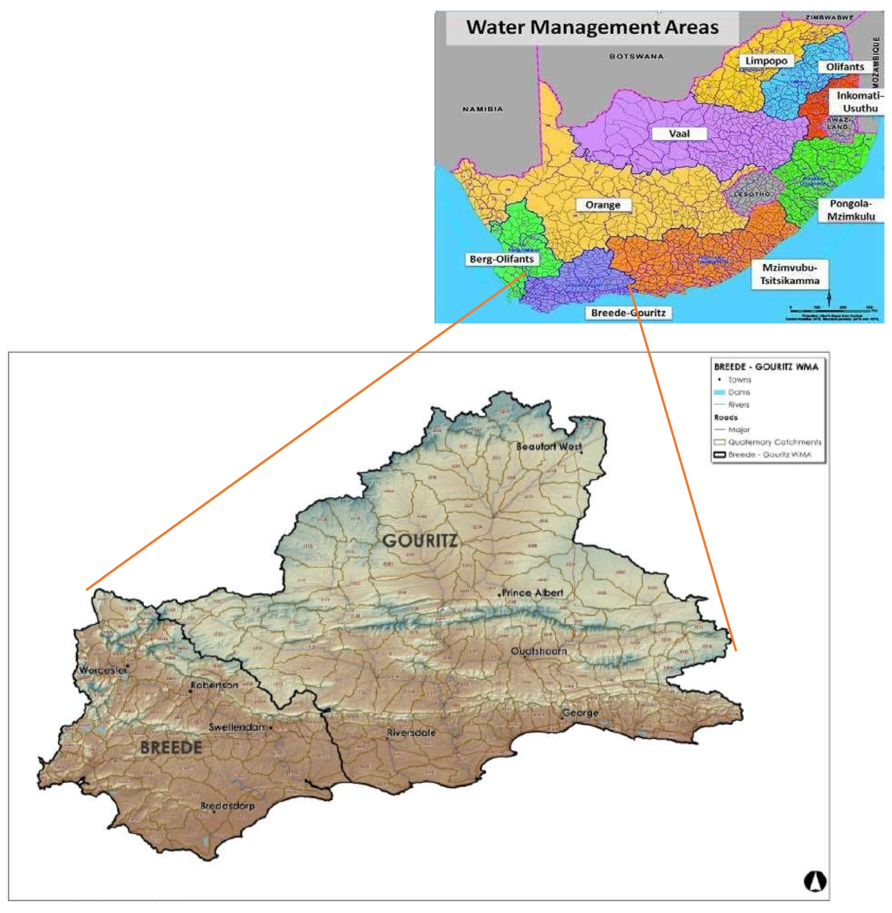
Figure 2.
Land cover maps according to the simplified ten land cover classes for 1990 (a), 2013/14 (b) and 2020 (c) maps, respectively. 3.2 Data analysis.
Figure 2.
Land cover maps according to the simplified ten land cover classes for 1990 (a), 2013/14 (b) and 2020 (c) maps, respectively. 3.2 Data analysis.
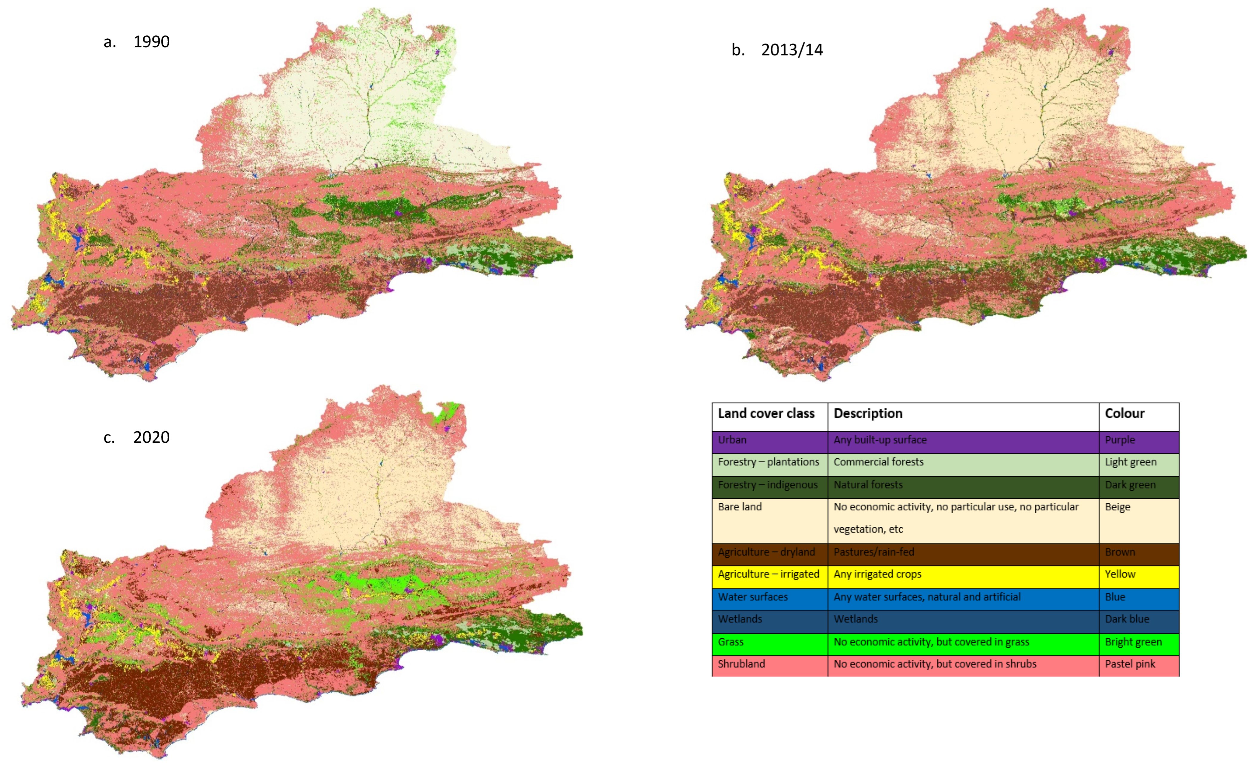
Figure 3.
Map of different climate zones according to the Köppen-Geiger classification (Beck et al., 2020). Large purple circles represent selected weather stations. Smaller black triangles represent the selected boreholes.
Figure 3.
Map of different climate zones according to the Köppen-Geiger classification (Beck et al., 2020). Large purple circles represent selected weather stations. Smaller black triangles represent the selected boreholes.
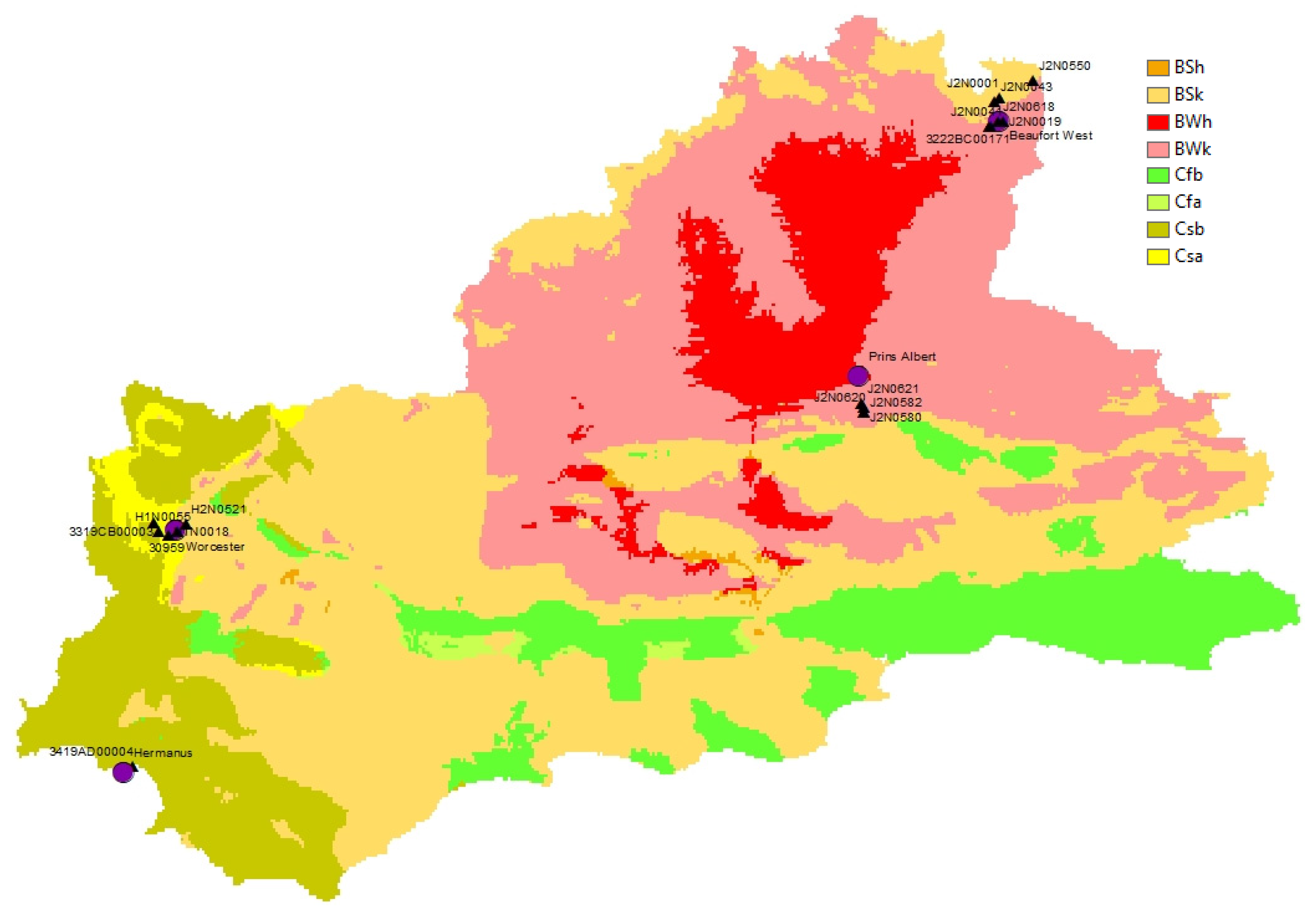
Figure 4.
A flowchart of the change detection analysis process and methods that were employed.
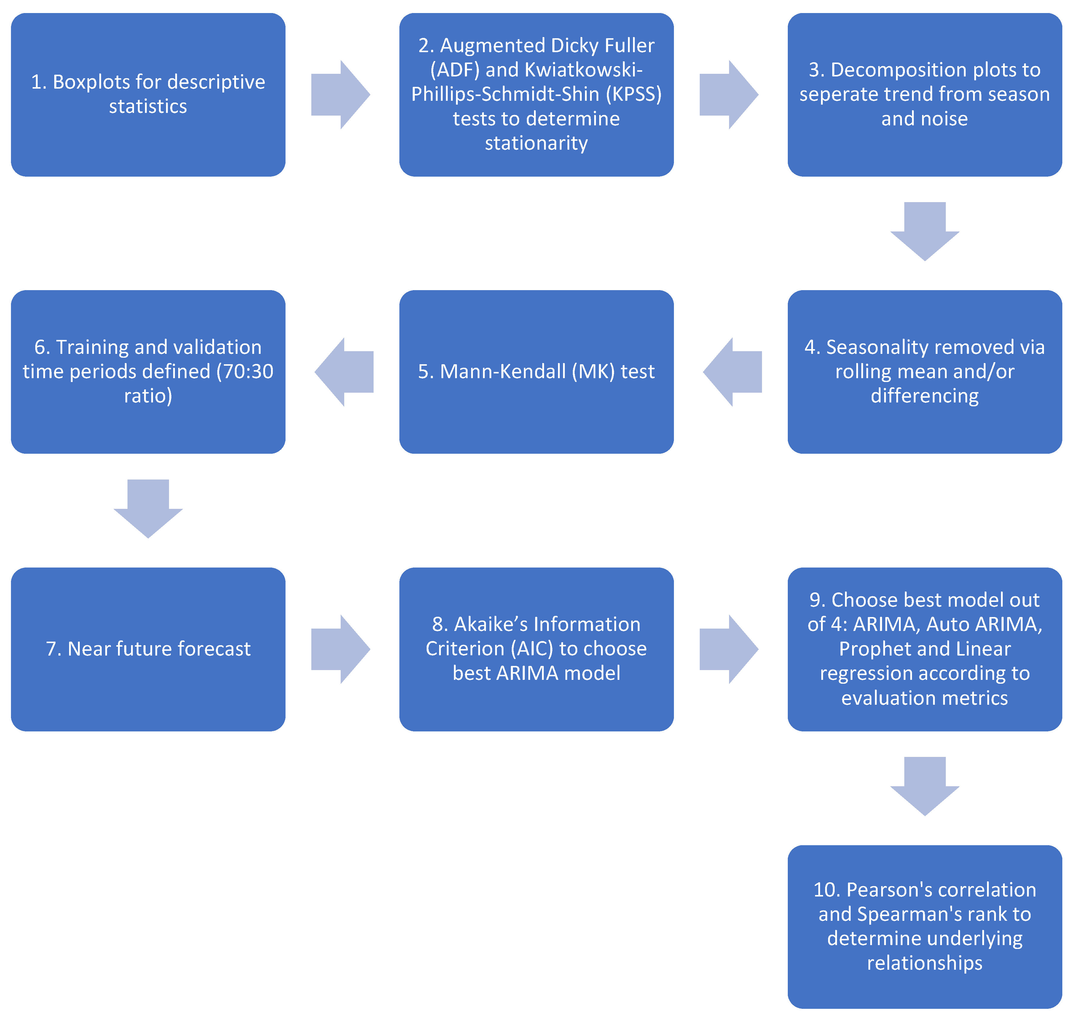
Figure 5.
Decomposition plots for average temperature (°C), monthly precipitation sum (mm), monthly evapotranspiration (mm), and groundwater depth (m) from boreholes J2N0580 and J2N0620 in the BWh subregion.
Figure 5.
Decomposition plots for average temperature (°C), monthly precipitation sum (mm), monthly evapotranspiration (mm), and groundwater depth (m) from boreholes J2N0580 and J2N0620 in the BWh subregion.
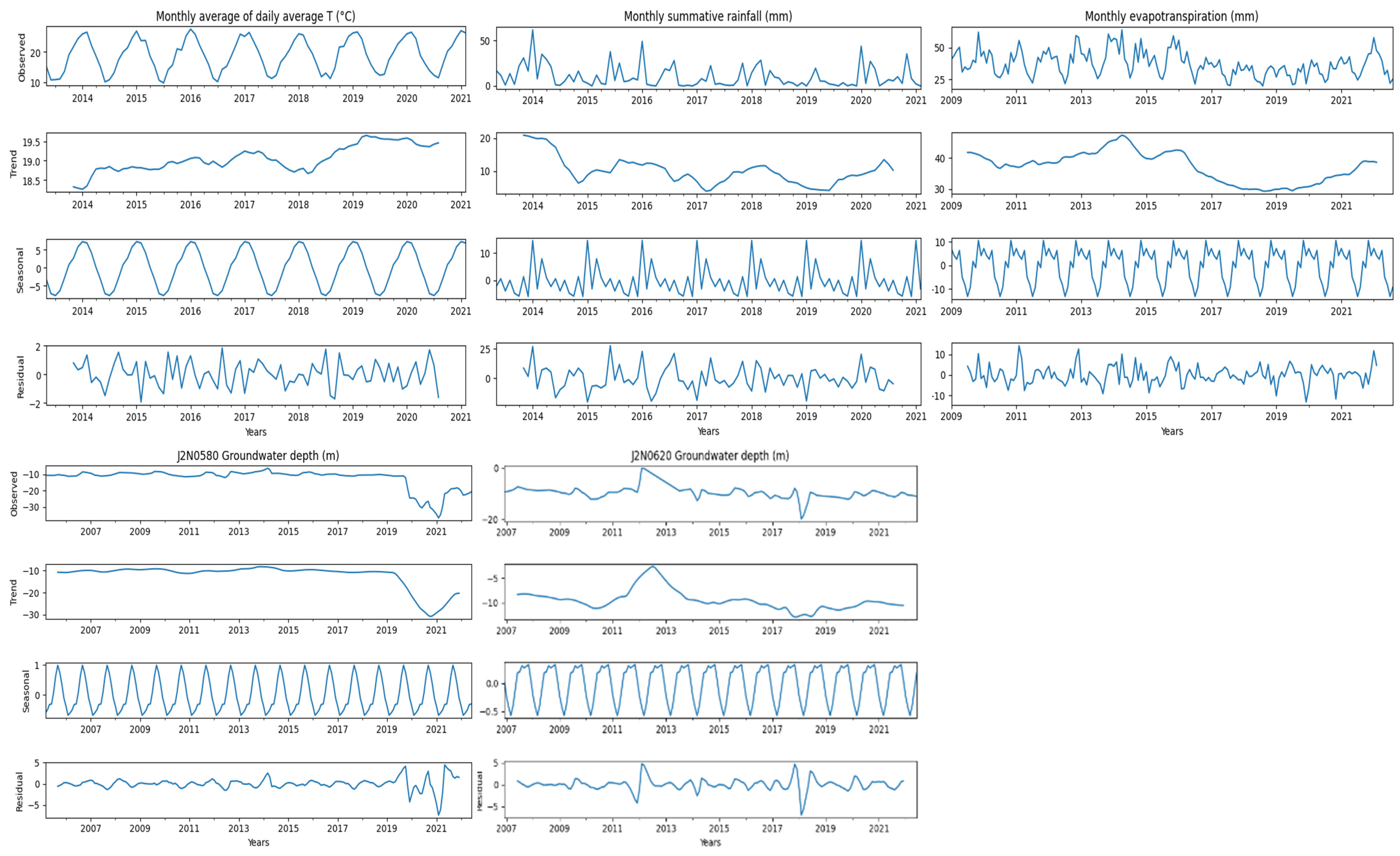
Figure 6.
a. Forecasts for Prins Albert T, P, ET and GWD from borehole J2N0580 in the BWh subregion, respectively. The dark blue line represents the validation data, and the lighter blue line represents the training data. The black/red line, depending on the respective model, displays the forecast for the validation period. The grey/green line, depending on the respective model, indicates the forecast for the entire period. b. Forecasts for Prins Albert GWD from boreholes J2N0582, J2N0620, and J2N0621 in the BWh subregion, respectively. The black/red line, depending on the respective model, displays the forecast for the validation period. The grey/green line, depending on the respective model, indicates the forecast for the entire period.
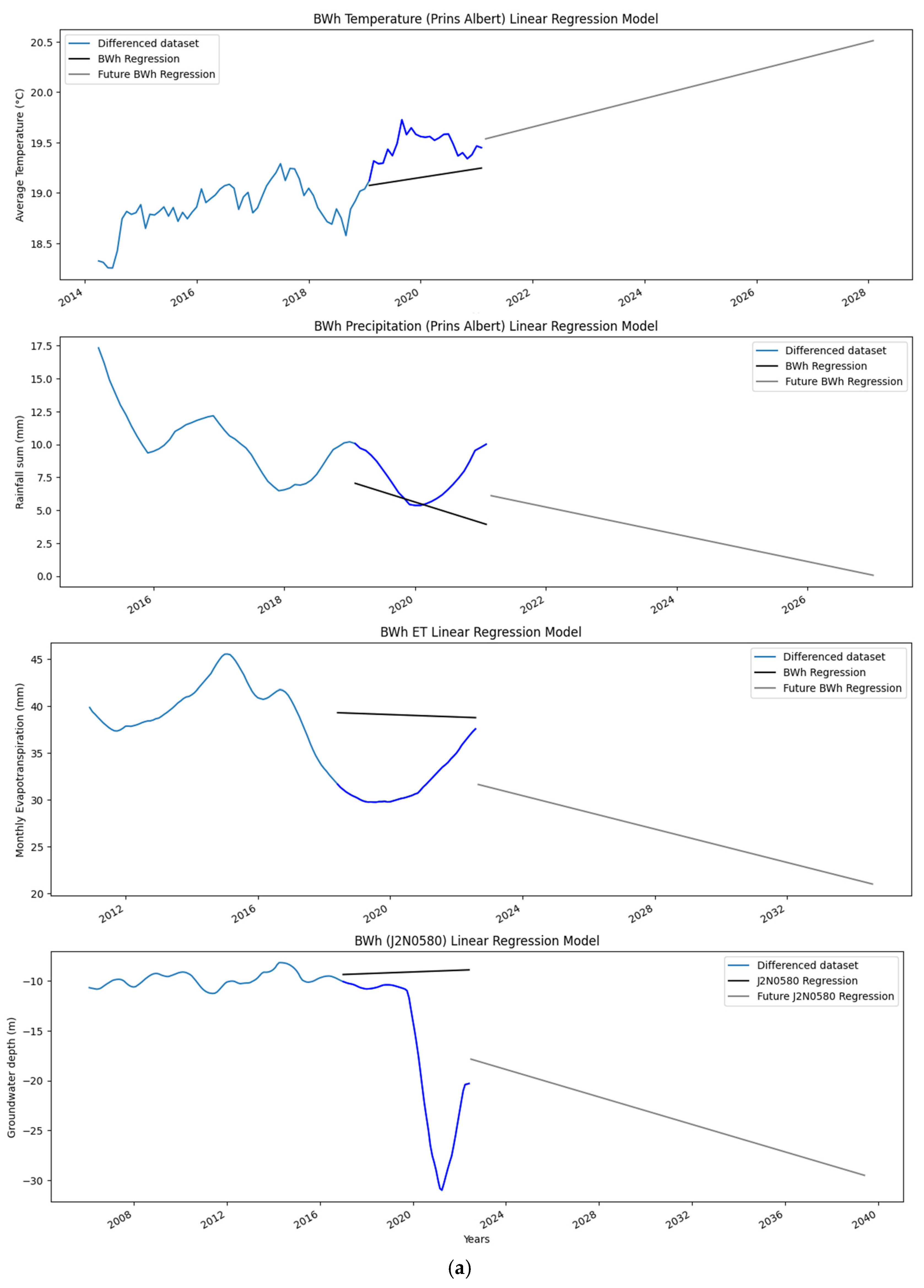
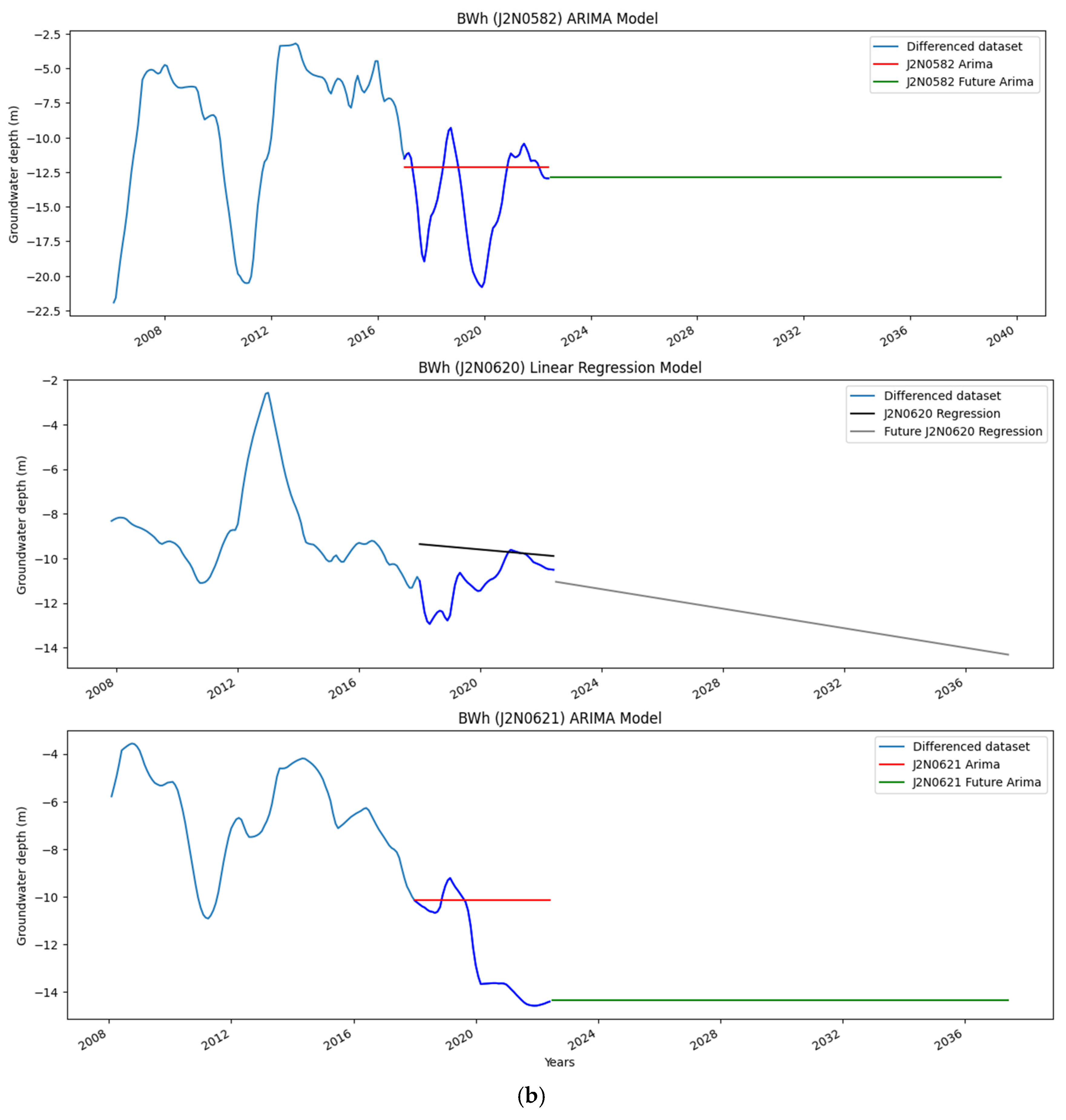
Figure 7.
Decomposition plots for average temperature (°C), monthly precipitation sum (mm), monthly evapotranspiration (mm), and groundwater depth (m) from boreholes 3222BC00179, J2N0001 and J2N0043 in the BWk subregion.
Figure 7.
Decomposition plots for average temperature (°C), monthly precipitation sum (mm), monthly evapotranspiration (mm), and groundwater depth (m) from boreholes 3222BC00179, J2N0001 and J2N0043 in the BWk subregion.
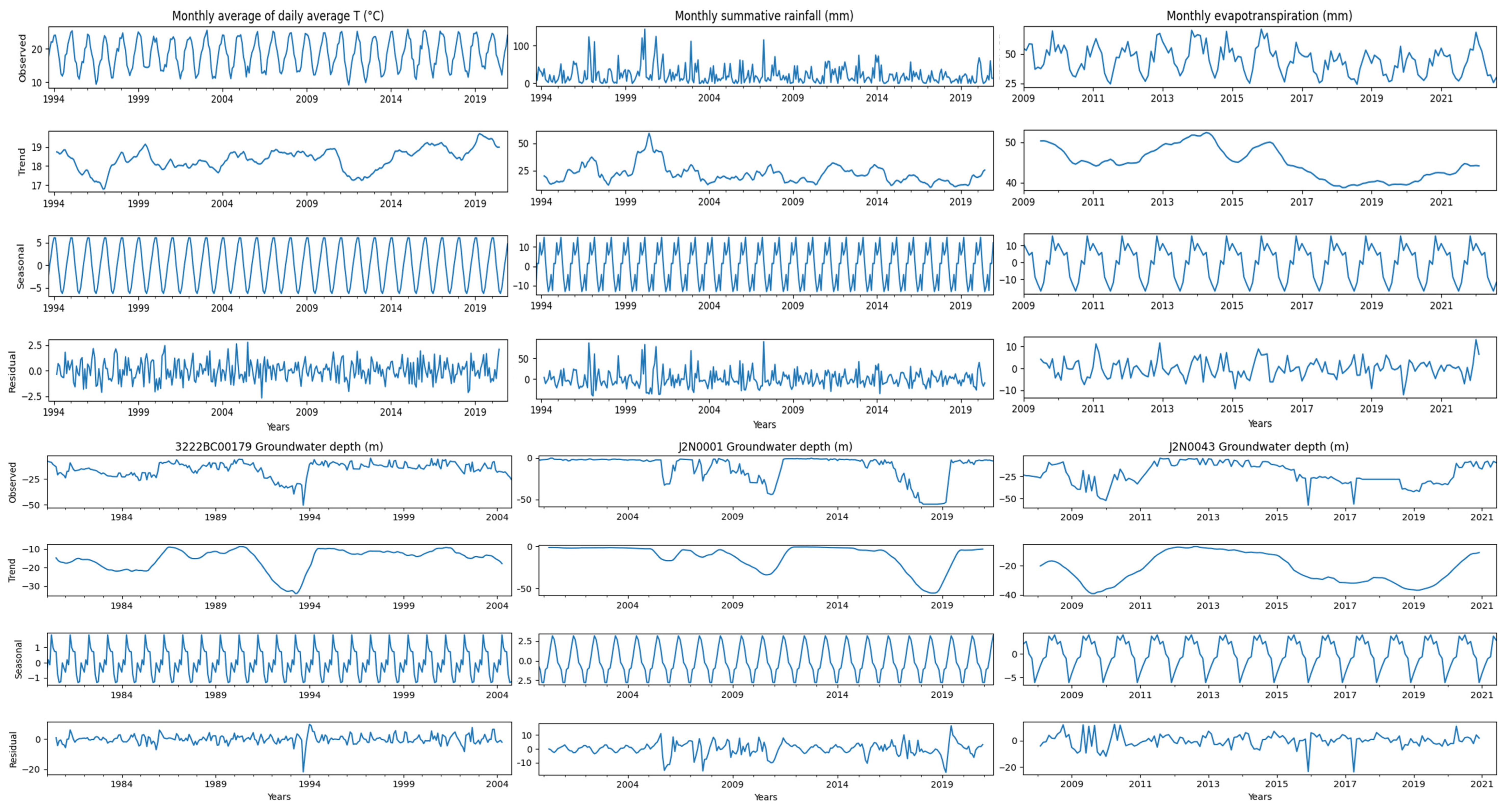
Figure 8.
a. Forecasts for Beaufort West T, P, ET and GWD for borehole 3222BC00170 in the BWk subregion, respectively. The dark blue line represents the validation data, and the lighter blue line represents the training data. Depending on the respective model, the black/pink/red/orange line displays the forecast for the validation period. Depending on the respective model, the grey/lime green/yellow/green line indicates the forecast for the entire period. b. Forecasts for GWD for boreholes 3222BC00179, 3222BC00152, 3222BC00171 and J2N0001 in the BWk subregion, respectively. The dark blue line represents the validation data, and the lighter blue line represents the training data. Depending on the respective model, the black/pink/red/orange line displays the forecast for the validation period. Depending on the respective model, the grey/lime green/yellow/green line indicates the forecast for the entire period. c. Forecasts for GWD for boreholes J2N0019, J2N0041, J2N0043 and J2N0550 in the BWk subregion, respectively. The dark blue line represents the validation data, and the lighter blue line represents the training data. Depending on the respective model, the black/pink/red/orange line displays the forecast for the validation period. Depending on the respective model, the grey/lime green/yellow/green line indicates the forecast for the entire period. d. Forecasts for GWD for borehole J2N0618 in the BWk subregion. The dark blue line represents the validation data, and the lighter blue line represents the training data. Depending on the respective model, the black/pink/red/orange line displays the forecast for the validation period. Depending on the respective model, the grey/lime green/yellow/green line indicates the forecast for the entire period.
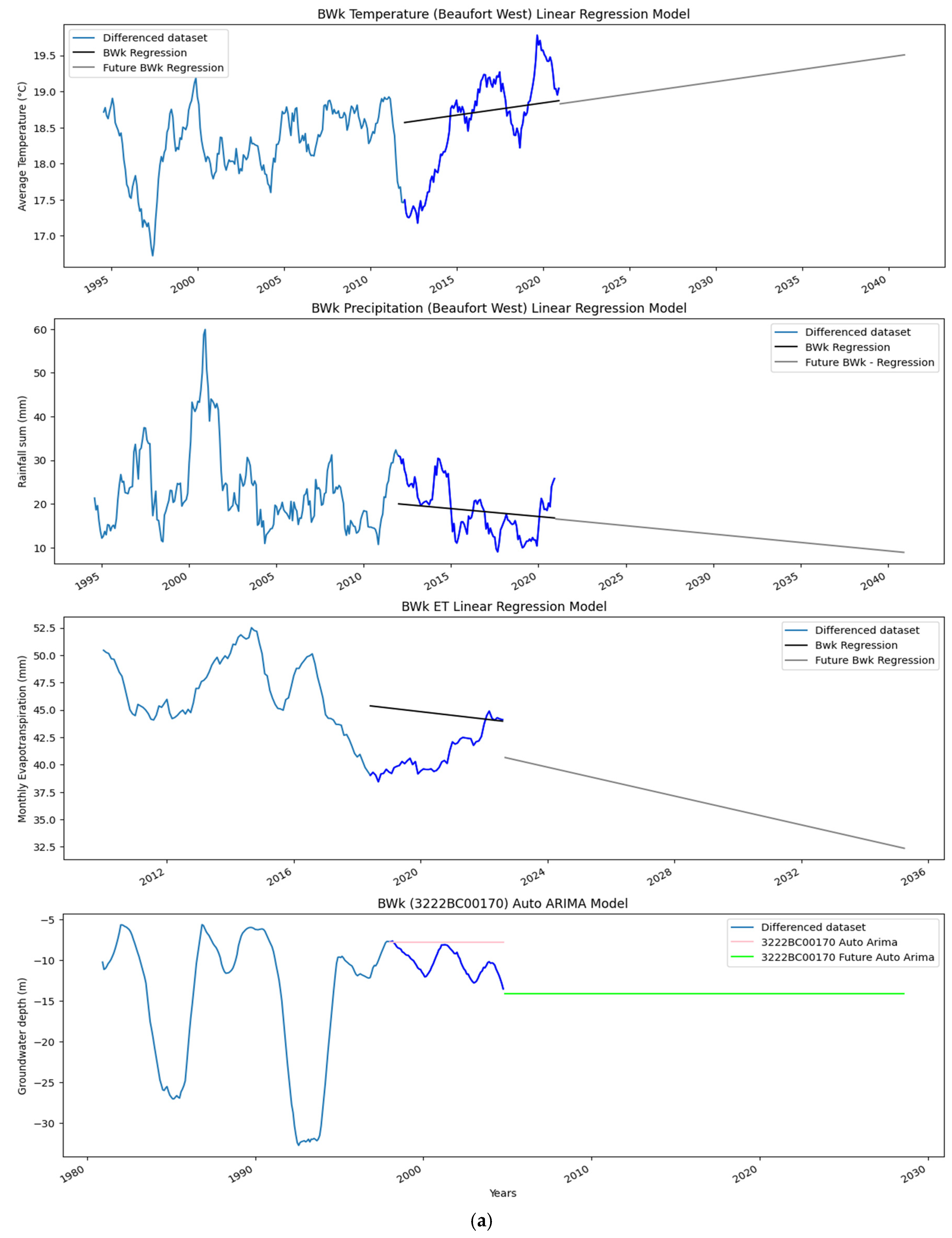
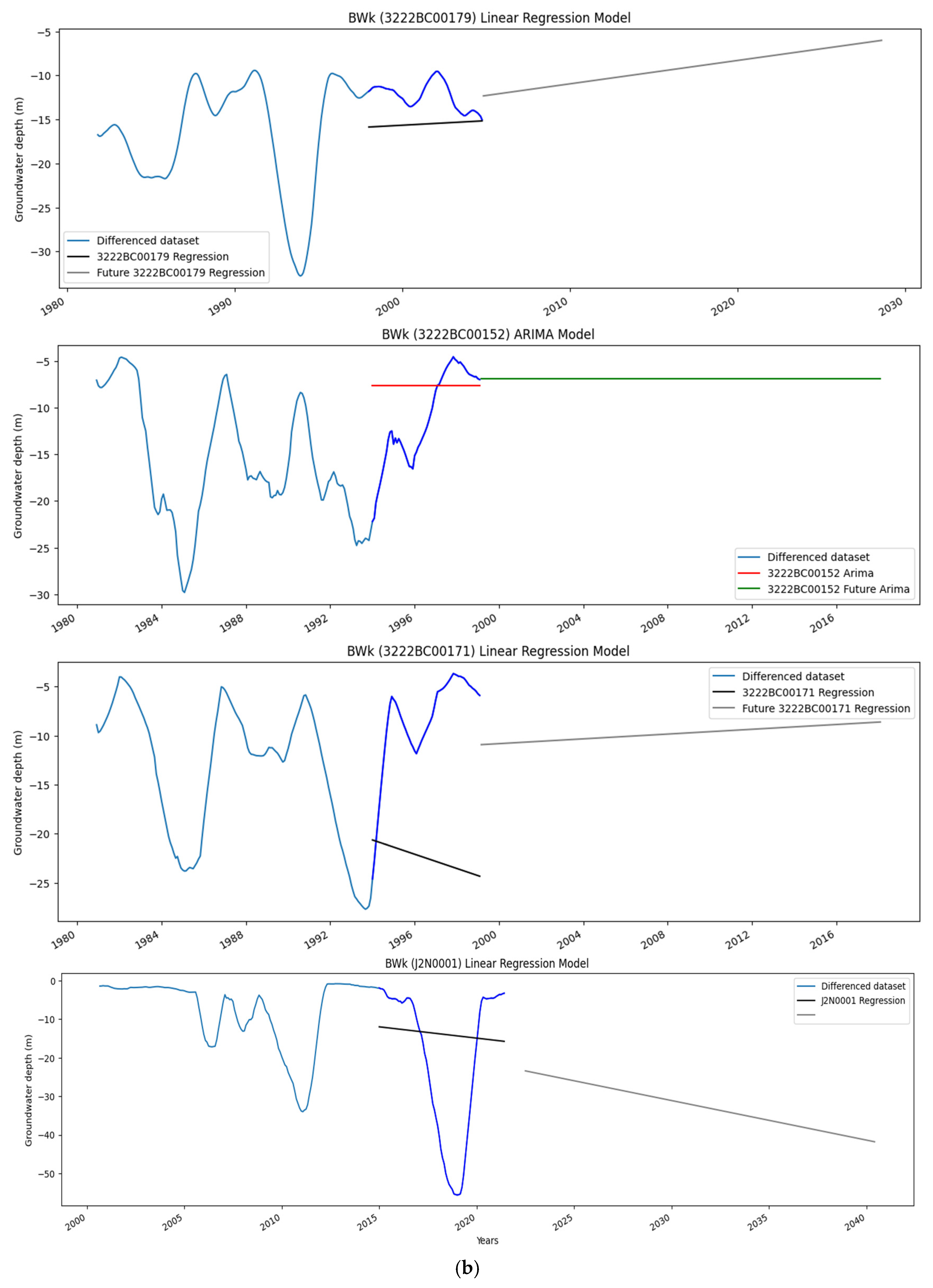
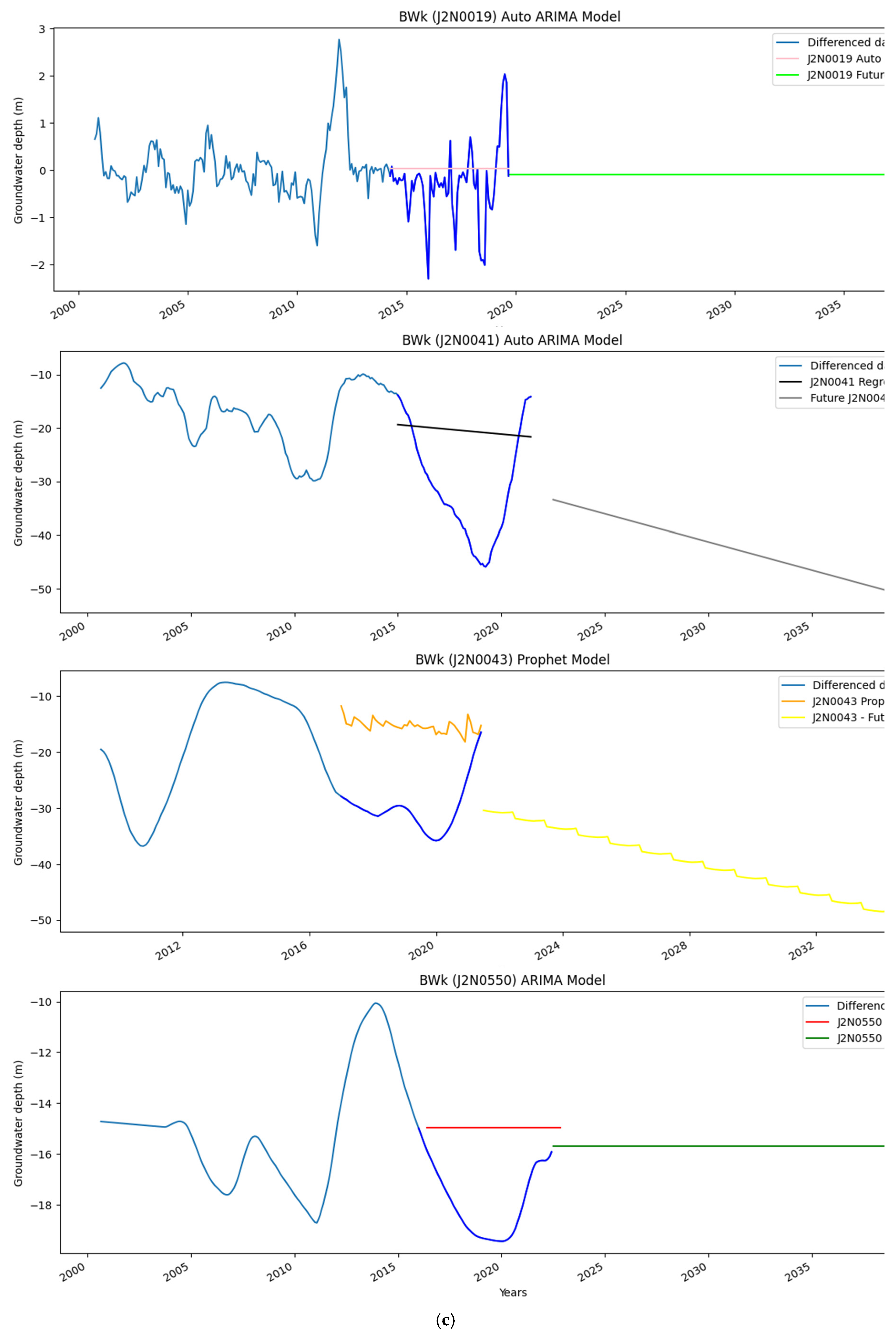
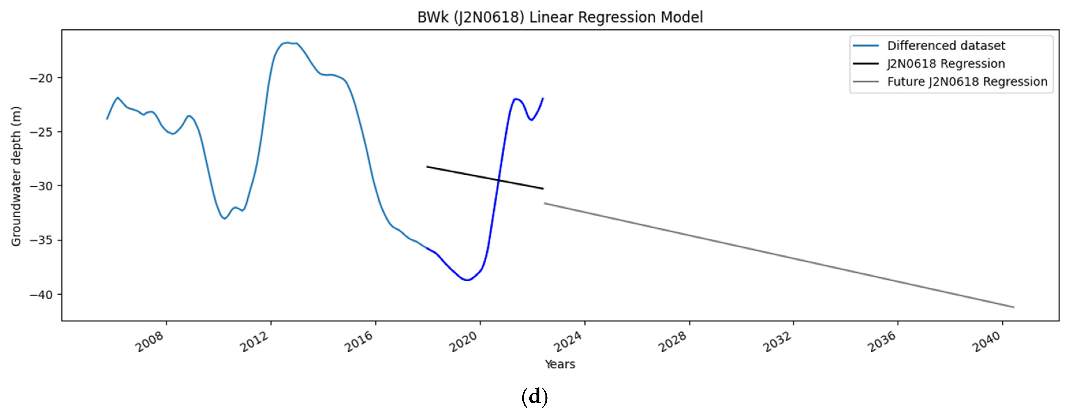
Figure 9.
Decomposition plots for average temperature (°C), monthly precipitation sum (mm), monthly evapotranspiration (mm), and groundwater depth (m) from borehole 3419AD00004 in the Csb subregion.
Figure 9.
Decomposition plots for average temperature (°C), monthly precipitation sum (mm), monthly evapotranspiration (mm), and groundwater depth (m) from borehole 3419AD00004 in the Csb subregion.
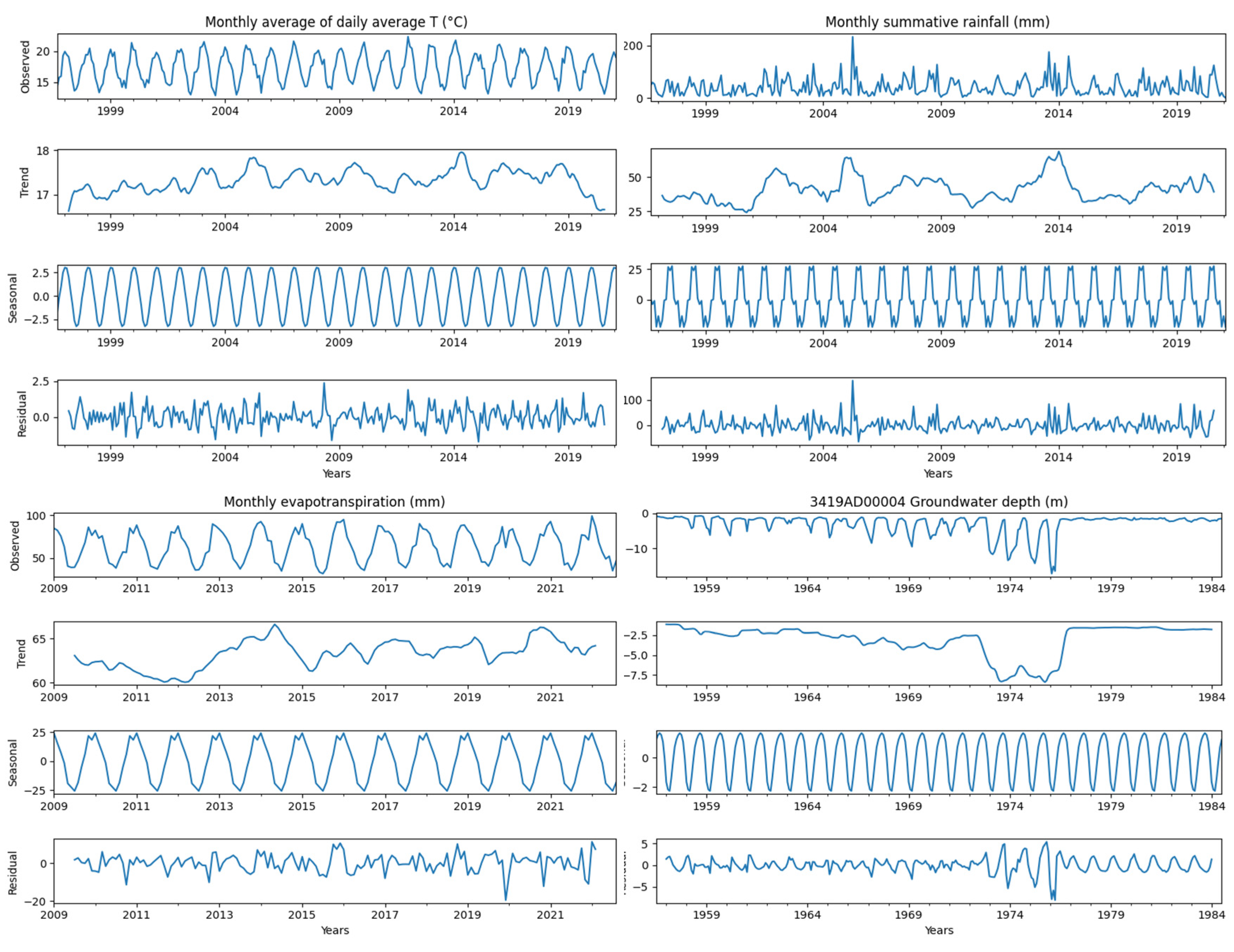
Figure 10.
a. Forecasts for T, P, and ET in the Csb subregion, respectively. The dark blue line represents the validation data, and the lighter blue line represents the training data. The black/red line, depending on the respective model, displays the forecast for the validation period. The grey/green line, depending on the respective model, indicates the linear regression forecast for the entire period. b. Forecasts for GWD for borehole 3419AD00004 in the Csb subregion, respectively. The dark blue line represents the validation data, and the lighter blue line represents the training data. The black/red line, depending on the respective model, displays the forecast for the validation period. The grey/green line, depending on the respective model, indicates the linear regression forecast for the entire period.
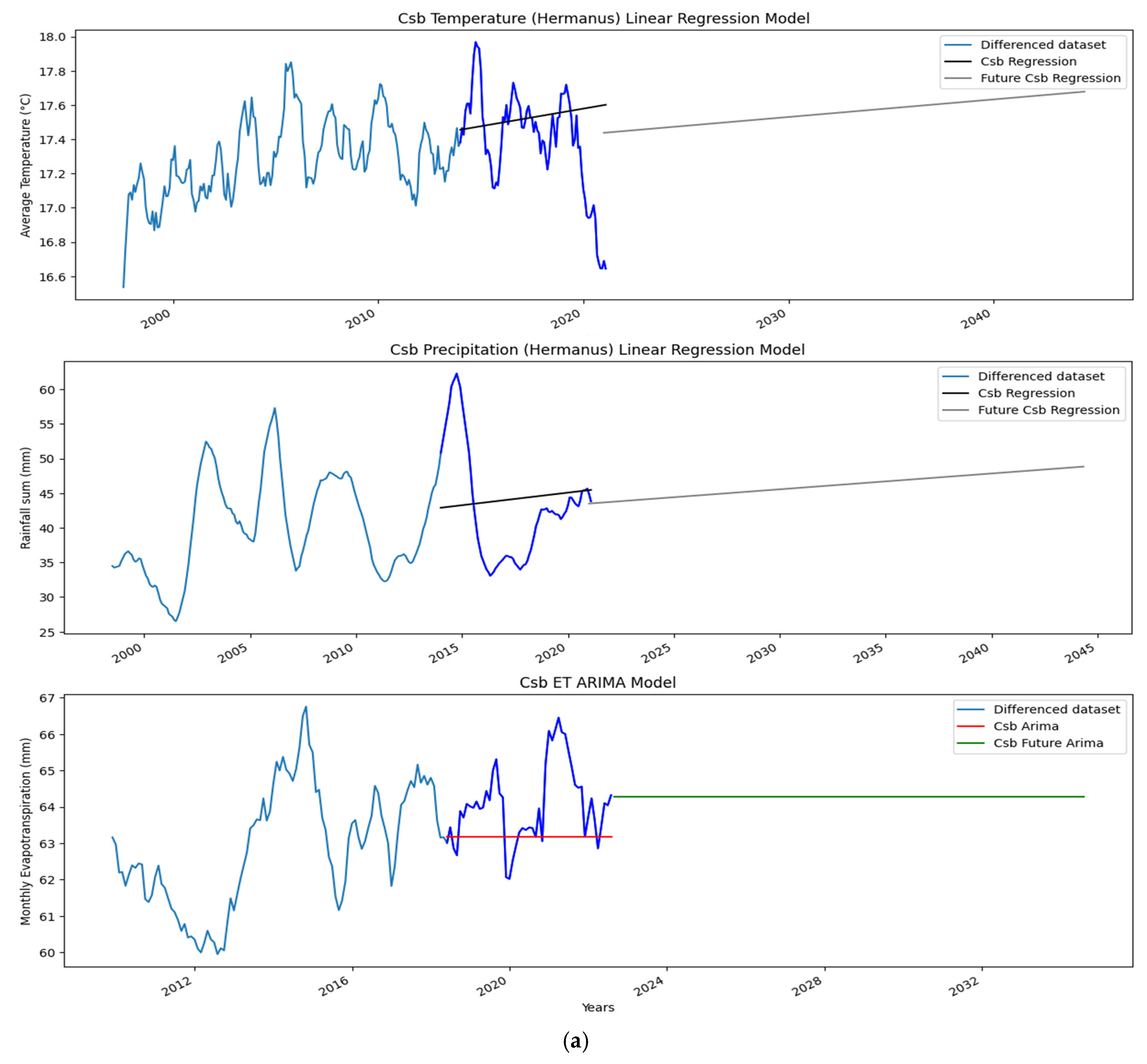
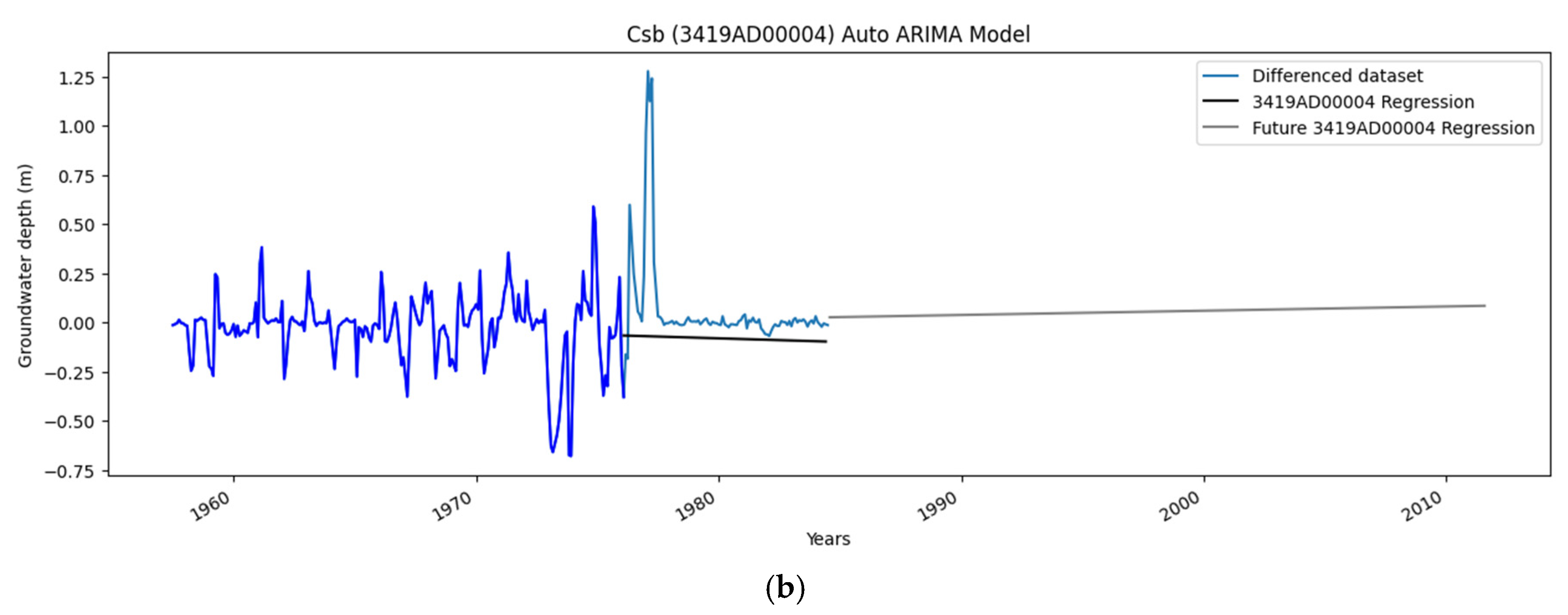
Figure 11.
Decomposition plots for average temperature (°C), monthly precipitation sum (mm), monthly evapotranspiration (mm), and groundwater depth (m) from boreholes 30,959 and H2N0521 in the Csa subregion.
Figure 11.
Decomposition plots for average temperature (°C), monthly precipitation sum (mm), monthly evapotranspiration (mm), and groundwater depth (m) from boreholes 30,959 and H2N0521 in the Csa subregion.
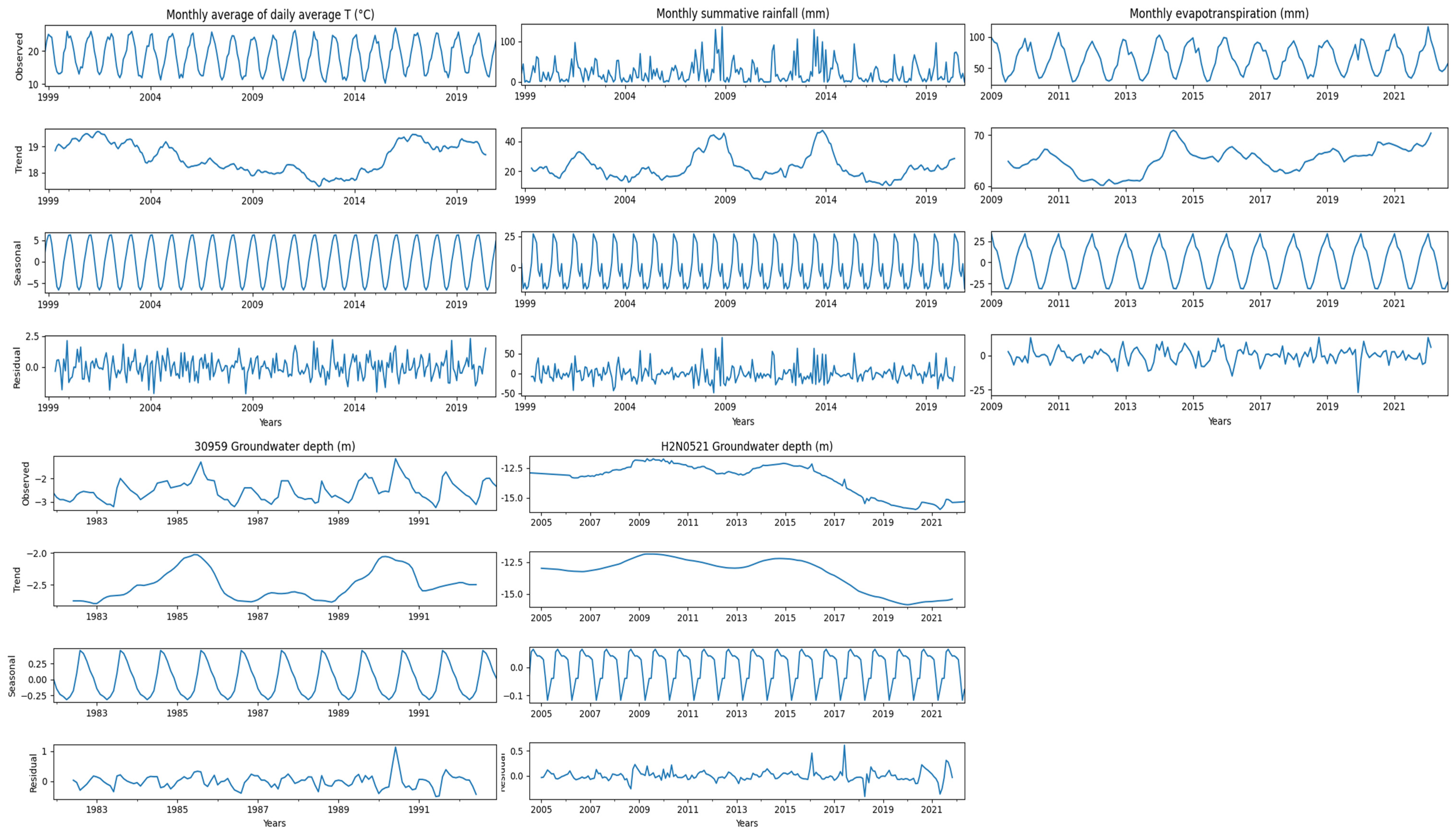
Figure 12.
a. Forecasts for Worcester T, P, ET and GWD for borehole 30,959 in the Csa subregion, respectively. The dark blue line represents the validation data, and the lighter blue line represents the training data. Depending on the respective model, the black/orange/pink line displays the forecast for the validation period. Depending on the respective model, the grey/lime green/yellow line indicates the forecast for the entire period. b. Forecasts for GWD for boreholes 3319CB00015, 3319CB00003, H1N0018 and H1N0055 in the Csa subregion, respectively. The dark blue line represents the validation data, and the lighter blue line represents the training data. Depending on the respective model, the black/orange/pink line displays the forecast for the validation period. Depending on the respective model, the grey/lime green/yellow line indicates the forecast for the entire period. c. Forecasts for GWD for borehole H2N0521 in the Csa subregion, respectively. The dark blue line represents the validation data, and the lighter blue line represents the training data. Depending on the respective model, the black/orange/pink line displays the forecast for the validation period. Depending on the respective model, the grey/lime green/yellow line indicates the forecast for the entire period.
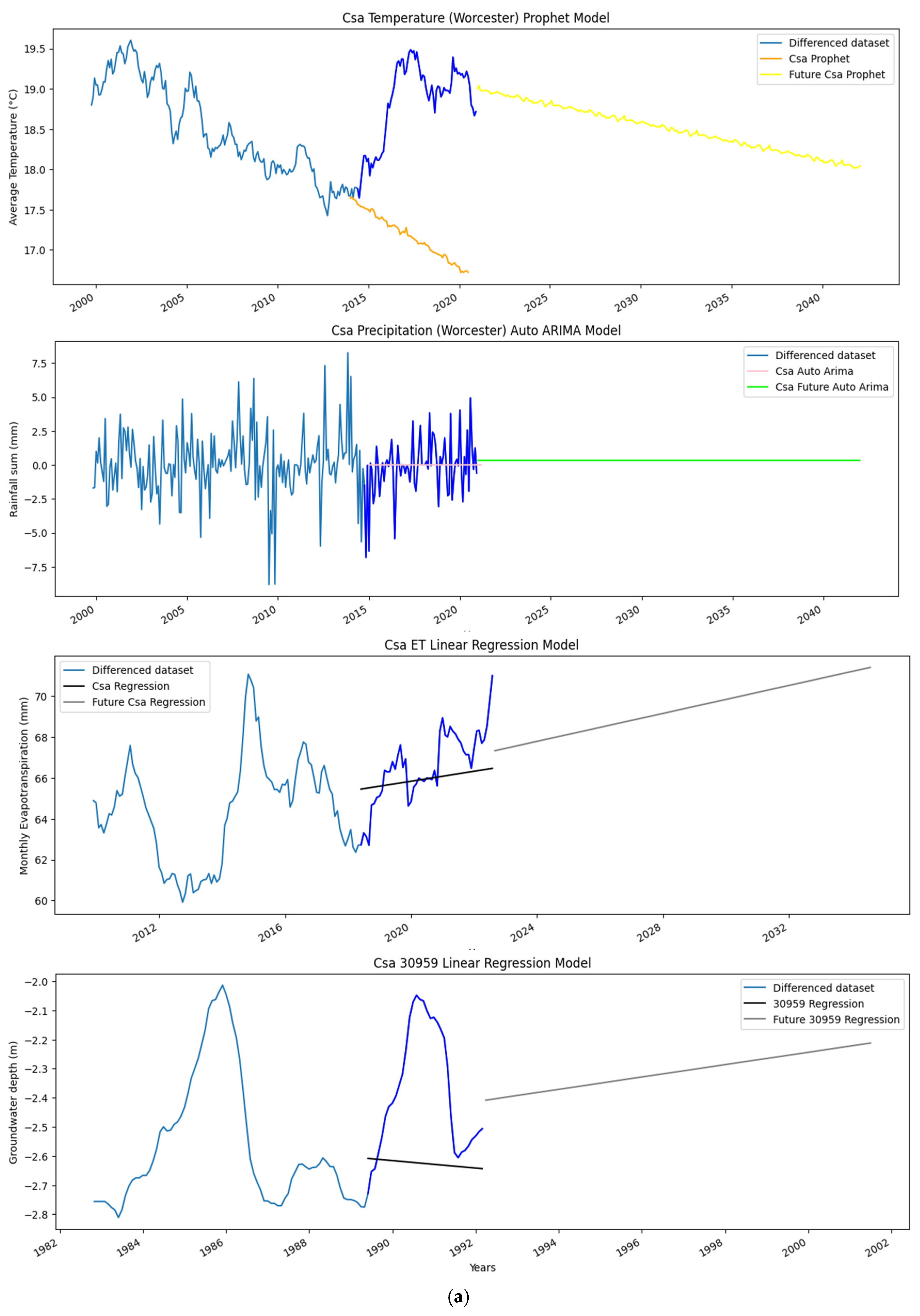
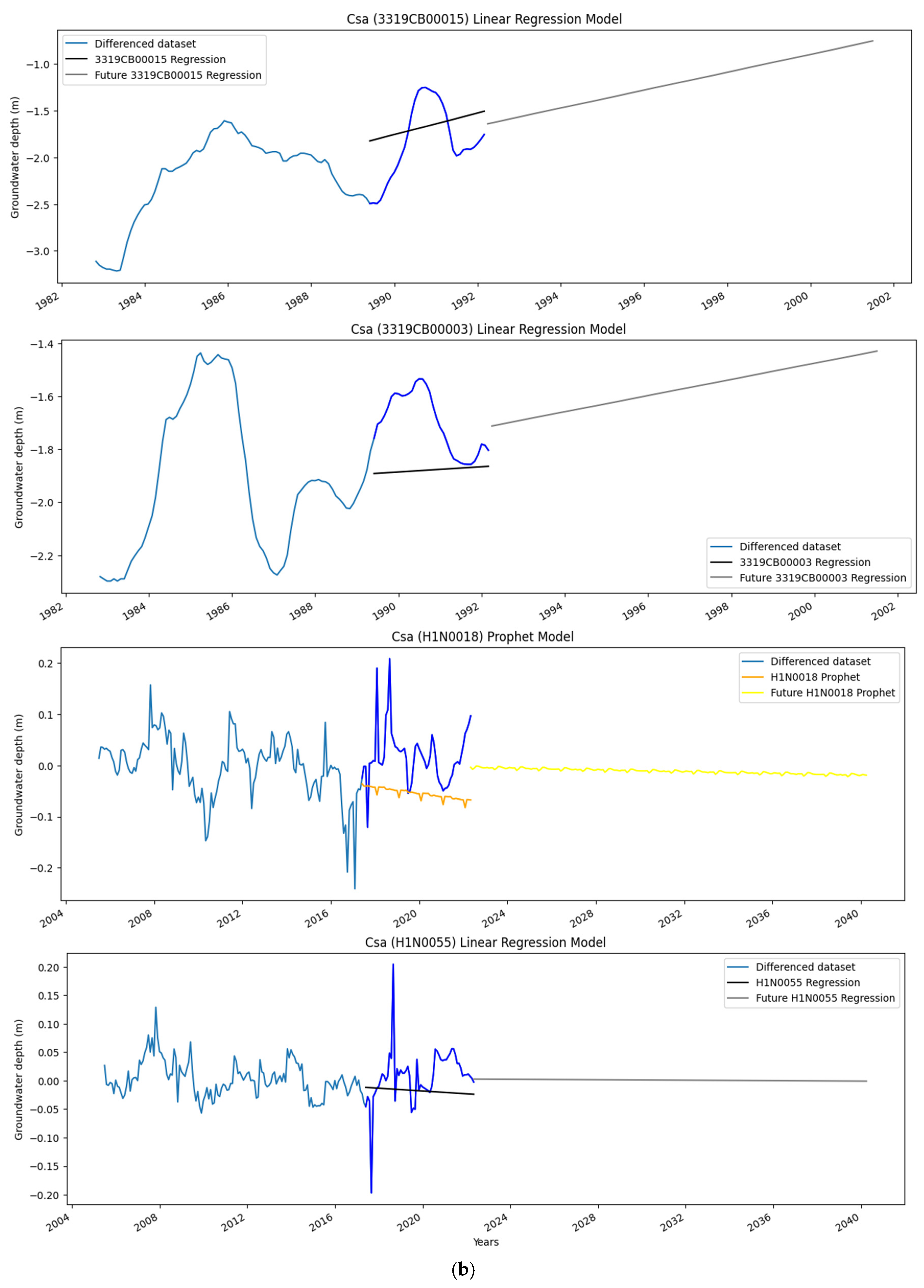
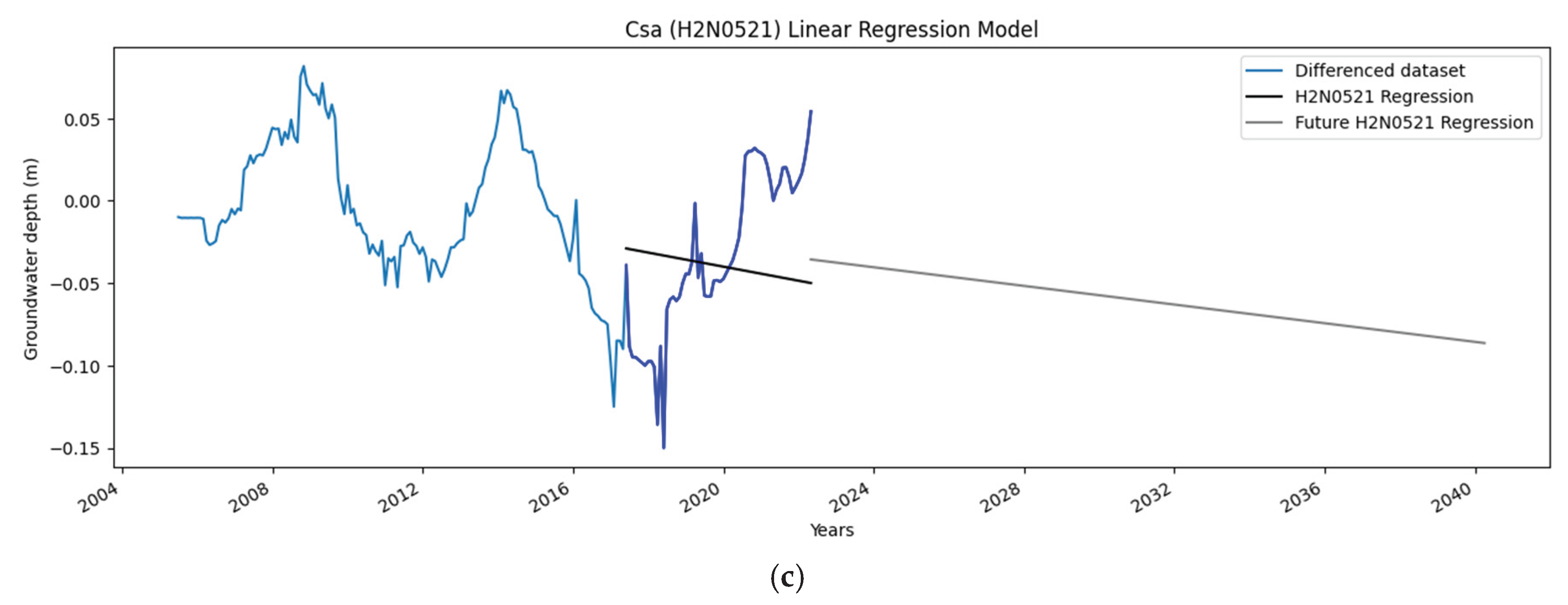

Table 1.
Boreholes chosen for further analysis, the period for which data were available to analyse and the forecast period.
Table 1.
Boreholes chosen for further analysis, the period for which data were available to analyse and the forecast period.
| NGA | |||||||
| Station | Borehole ID | Subregion according to Köppen-Geiger classification | Period analysed | Forecast period | Distance and direction from the station | Elevation (m) | Usage status |
| Beaufort-West | 3222BC00170 | BWk | 1980 - 2004 | 2004 - 2028 | 4.71km SW | 860 | Measurements ceased after 2004 |
| 3222BC00179 | 1980 - 2004 | 2004 - 2028 | 4.71 km SW | 860 | |||
| 3222BC00152 | 1980 - 1999 | 1999 - 2018 | 0.45 km SW | 860 | Abandoned | ||
| 3222BC00171 | 1980 - 1999 | 1999 - 2018 | 4.71 km SW | 860 | |||
| Hermanus | 3419AD00004 | Csb | 1956 - 1984 | 1984 - 2012 | 4.73 km NE | 20 | Abandoned |
| Worcester | 30959 | Csa | 1982 - 1992 | 1992 - 2002 | 3.84 km SW | 205 | In use: unknown consumer (the old H1N0018) |
| 3319CB00015 | 1982 - 1992 | 1992 - 2002 | 10.15 km NW | 209 | Abandoned | ||
| 3319CB00003 | 1982 - 1992 | 1992 - 2002 | 7.09 km W | 204 | |||
| HYDSTRA | |||||||
| Beaufort West | J2N0001 | BWk | 1963-2021 | 2022-2042 | 10.1 km N | 944 | Local municipal use |
| J2N0019 | 1974-2019 | 2020-2038 | 1.46 km E | 852 | |||
| J2N0041 | 1974-2021 | 2022-2042 | 4.66 km SW | 860 | |||
| J2N0043 | 2007-2021 | 2022-2042 | 9.1 km NNW | 1074 | |||
| J2N0550 | 1975- present | 2022-2042 | 22.56 km NE | 979 | In use: Unknown consumer | ||
| J2N0618 | 2004-present | 2022-2042 | 0.97 WNW | 869 | |||
| Prins Albert | J2N0580 | BWh | 2005-2022 | 2022-2040 | 13.1 km S | 705 | In use: Unknown consumer |
| J2N0582 | 2005-2022 | 2022-2040 | 15.46 km S | 762 | |||
| J2N0620 | 2006-2022 | 2022-2038 | 15.6 km S | 742 | |||
| J2N0621 | 2007-2022 | 2022-2038 | 11.29 km S | 674 | |||
| Worcester | H1N0018 | Csa | 1981-2022 | 2022-2040 | 3.84 km SW | 205 | In use: Unknown consumer |
| H1N0055 | 1978-2022 | 1.02 km SE | 209 | ||||
| H2N0521 | 2004-2022 | 5.24 km NE | 247 | ||||
Table 2.
Pearson and Spearman’s rank correlation test results for temperature (T), precipitation (P), evapotranspiration (ET) and groundwater depth (GWD) (J2N0580, J2N0582, J2N0620, J2N0621) variables in the BWh subregion.
Table 2.
Pearson and Spearman’s rank correlation test results for temperature (T), precipitation (P), evapotranspiration (ET) and groundwater depth (GWD) (J2N0580, J2N0582, J2N0620, J2N0621) variables in the BWh subregion.
| Pearson’s | |||||||
| T | P | ET | J2N0580 | J2N0582 | J2N0620 | J2N0621 | |
| T | 1 | 0.16 | 0.52 | -0.14 | 0.0014 | -0.2 | 0.05 |
| P | 0.16 | 1 | 0.34 | 0.059 | 0.31 | 0.039 | 0.18 |
| ET | 0.52 | 0.34 | 1 | 0.18 | 0.36 | 0.2 | 0.5 |
| J2N0580 | -0.14 | 0.059 | 0,18 | 1 | 0.079 | -0.082 | 0.67 |
| J2N0582 | 0.0014 | 0.31 | 0.36 | 0.079 | 1 | 0.38 | 0.46 |
| J2N0620 | -0.2 | 0.039 | 0.2 | -0.082 | 0.38 | 1 | 0.32 |
| J2N0621 | 0.05 | 0.18 | 0.5 | 0.67 | 0.46 | 0.32 | 1 |
| Spearman’s rank | |||||||
| T | P | ET | J2N0580 | J2N0582 | J2N0620 | J2N0621 | |
| T | 1 | 0.046 | 0.57 | -0.07 | -0.1 | -0.2 | 0.017 |
| P | 0.046 | 1 | 0.24 | 0.23 | 0.35 | 0.29 | 0.2 |
| ET | 0.57 | 0.24 | 1 | 0.41 | 0.33 | 0.25 | 0.43 |
| J2N0580 | -0.07 | 0.23 | 0.41 | 1 | 0.48 | 0.36 | 0.9 |
| J2N0582 | -0.1 | 0.35 | 0.33 | 0.48 | 1 | 0.73 | 0.51 |
| J2N0620 | -0.2 | 0.29 | 0.25 | 0.36 | 0.73 | 1 | 0.43 |
| J2N0621 | 0.017 | 0.2 | 0.43 | 0.9 | 0.51 | 0.43 | 1 |
Table 3.
Mann-Kendall (MK) test results for temperature (T), precipitation (P), evapotranspiration (ET) and groundwater depth (GWD) (J2N0580, J2N0582, J2N0620, J2N0621) variables in the BWh subregion. The tuple consists of the trend, the h-value (true/false if a trend is present), the p-value, the slope (Theil-Sen estimator/slope) and the intercept (intercept of Kendall-Theil Robust Line).
| MK test results | ||||||
| Trend | h | p | Slope | Intercept | ||
| T | ‘Increasing’ | True | 4.44 | 0.01 | 18.55 | |
| P | ‘decreasing’ | True | 3.23 | -0.08 | 12.70 | |
| ET | ‘decreasing’ | True | 1.83 | -0.07 | 42.73 | |
| Hydstra GWD | J2N0580 | ‘lowering’ | True | 7.01 | -0.01 | -9.12 |
| J2N0582 | ‘lowering’ | True | 1.72 | - 0.04 | -6.68 | |
| J2N0620 | ‘lowering’ | True | 4.44 | -0.02 | -8.44 | |
| J2N0621 | ‘lowering’ | True | 0.0 | -0.06 | -2.40 | |
Table 4.
Pearson and Spearman’s rank correlation test results for temperature (T), precipitation (P), and groundwater depth (GWD) (3222BC00170, 3222BC00179, 3222BC00152 and 3222BC00171) variables in the BWk subregion.
Table 4.
Pearson and Spearman’s rank correlation test results for temperature (T), precipitation (P), and groundwater depth (GWD) (3222BC00170, 3222BC00179, 3222BC00152 and 3222BC00171) variables in the BWk subregion.
| Pearson’s | ||||||
| T | P | 3222BC00170 | 3222BC00179 | 3222BC00152 | 3222BC00171 | |
| T | 1 | 0.25 | -0.18 | -0.084 | -0.31 | -0.17 |
| P | 0.25 | 1 | -0.055 | 0.0054 | -0.051 | -0.17 |
| 3222BC00170 | -0.18 | -0.055 | 1 | 0.85 | 0.61 | 0.92 |
| 3222BC00179 | -0.084 | 0.0054 | 0.85 | 1 | 0.33 | 0.71 |
| 3222BC00152 | -0.31 | -0.051 | 0.61 | 0.33 | 1 | 0.71 |
| 3222BC00171 | -0.17 | -0.17 | 0.92 | 0.71 | 0.71 | 1 |
| Spearman’s | ||||||
| T | P | 3222BC00170 | 3222BC00179 | 3222BC00152 | 3222BC00171 | |
| T | 1 | 0.3 | -0.23 | -0.14 | -0.28 | -0.18 |
| P | 0.3 | 1 | -0.15 | -0.023 | -0.2 | -0.31 |
| 3222BC00170 | -0.23 | -0.15 | 1 | 0.68 | 0.63 | 0.8 |
| 3222BC00179 | -0.14 | -0.023 | 0.68 | 1 | -0.048 | 0.15 |
| 3222BC00152 | -0.28 | -0.2 | 0.63 | -0.048 | 1 | 0.77 |
| 3222BC00171 | -0.18 | -0.31 | 0.8 | 0.15 | 0.77 | 1 |
Table 5.
Pearson and Spearman’s rank correlation test results for temperature (T), precipitation (P), evapotranspiration (ET) and groundwater depth (GWD) (J2N0001, J2N0019, J2N0041, J2N0043, J2N0550 and J2N0618) variables in the BWk subregion.
Table 5.
Pearson and Spearman’s rank correlation test results for temperature (T), precipitation (P), evapotranspiration (ET) and groundwater depth (GWD) (J2N0001, J2N0019, J2N0041, J2N0043, J2N0550 and J2N0618) variables in the BWk subregion.
| Pearson’s | |||||||||
| T | P | ET | J2N0001 | J2N0019 | J2N0041 | J2N0043 | J2N0550 | J2N0618 | |
| T | 1 | 0.35 | 0.74 | -0.12 | -0.4 | -0.21 | -0.26 | -0.11 | -0.16 |
| P | 0.35 | 1 | 0.35 | 0.12 | 0.038 | 0.1 | 0.053 | 0.15 | 0.17 |
| ET | 0.74 | 0.35 | 1 | 0.12 | -0.062 | 0.1 | -0.063 | 0.24 | 0.13 |
| J2N0001 | -0.12 | 0.12 | 0.12 | 1 | 0.8 | 0.79 | 0.6 | 0.65 | 0.68 |
| J2N0019 | -0.4 | 0.038 | -0.062 | 0.8 | 1 | 0.84 | 0.7 | 0.76 | 0.77 |
| J2N0041 | -0.21 | 0.1 | 0.1 | 0.79 | 0.84 | 1 | 0.84 | 0.81 | 0.94 |
| J2N0043 | -0.26 | 0.053 | -0.063 | 0.6 | 0.7 | 0.84 | 1 | 0.72 | 0.85 |
| J2N0550 | -0.11 | 0.15 | 0.24 | 0.65 | 0.76 | 0.81 | 0.72 | 1 | 0.84 |
| J2N0618 | -0.16 | 0.17 | 0.13 | 0.68 | 0.77 | 0.94 | 0.85 | 0.84 | 1 |
| Spearman’s | |||||||||
| T | P | ET | J2N0001 | J2N0019 | J2N0041 | J2N0043 | J2N0550 | J2N0618 | |
| T | 1 | 0.3 | 0.74 | -0.12 | -0.41 | -0.22 | -0.26 | -0.095 | -0.16 |
| P | 0.3 | 1 | 0.26 | 0.12 | 0.065 | 0.074 | 0.062 | 0.14 | 0.13 |
| ET | 0.74 | 0.26 | 1 | 0.14 | -0.094 | 0.099 | -0.026 | 0.25 | 0.14 |
| J2N0001 | -0.12 | 0.12 | 0.14 | 1 | 0.86 | 0.85 | 0.77 | 0.77 | 0.82 |
| J2N0019 | -0.41 | 0.065 | -0.094 | 0.86 | 1 | 0.87 | 0.79 | 0.81 | 0.82 |
| J2N0041 | -0.22 | 0.074 | 0.099 | 0.85 | 0.87 | 1 | 0.87 | 0.83 | 0.95 |
| J2N0043 | -0.26 | 0.062 | -0.026 | 0.77 | 0.79 | 0.87 | 1 | 0.74 | 0.85 |
| J2N0550 | -0.095 | 0.14 | 0.25 | 0.77 | 0.81 | 0.83 | 0.74 | 1 | 0.86 |
| J2N0618 | -0.16 | 0.13 | 0.14 | 0.82 | 0.82 | 0.95 | 0.85 | 0.86 | 1 |
Table 6.
Mann-Kendall (MK) test results for temperature (T), precipitation (P), evapotranspiration (ET) and groundwater depth (GWD) (3222BC00170, 3222BC00179, 3222BC00152, 3222BC00171, J2N0001, J2N0019, J2N0041, J2N0043, J2N0550 and J2N0618 ) variables in the BWk subregion. The tuple consists of the trend, the h-value (true/false if a trend is present), the p-value, the slope (Theil-Sen estimator/slope) and the intercept (intercept of Kendall-Theil Robust Line).
| MK test results | ||||||
| Trend | h | p | Slope | Intercept | ||
| T | ‘Increasing’ | True | 0.0 | 0.003 | 17.93 | |
| P | ‘decreasing’ | True | 2.53 | -0.03 | 24.06 | |
| ET | ‘decreasing’ | True | 2.26 | -0.05 | 48.56 | |
| NGA GWD | 3222BC00170 | ‘no trend’ | False | 0.51 | -0.002 | -10.41 |
| 3222BC00179 | ‘rising’ | True | 3.42 | 0.02 | -15.71 | |
| 3222BC00152 | ‘no trend’ | False | 0.08 | 0.02 | -16.40 | |
| 3222BC00171 | ‘no trend’ | False | 0.07 | 0.01 | -11.25 | |
| Hydstra GWD | J2N0001 | ‘lowering’ | True | 5.73 | -0.04 | 0.43 |
| J2N0019 | ‘lowering’ | True | 0.02 | -0.001 | 0.009 | |
| J2N0041 | ‘lowering’ | True | 0.0 | -0.10 | -5.27 | |
| J2N0043 | ‘lowering’ | True | 2.49 | -0.10 | -19.16 | |
| J2N0550 | ‘lowering’ | True | 2.47 | -0.01 | -14.61 | |
| J2N0618 | ‘lowering’ | True | 6.69 | -0.06 | -18.81 | |
Table 7.
Pearson and Spearman’s rank correlation test results for temperature (T), precipitation (P), and evapotranspiration (ET) variables in the Csb subregion. No correlations could be made with GWD since the periods did not overlap.
Table 7.
Pearson and Spearman’s rank correlation test results for temperature (T), precipitation (P), and evapotranspiration (ET) variables in the Csb subregion. No correlations could be made with GWD since the periods did not overlap.
| Pearson’s | |||
| T | P | ET | |
| T | 1 | -0.6 | 0.86 |
| P | -0.6 | 1 | -0.52 |
| ET | 0.86 | -0.52 | 1 |
| Spearman’s | |||
| T | P | ET | |
| T | 1 | -0.65 | 0.84 |
| P | -0.65 | 1 | -0.59 |
| ET | 0.84 | -0.59 | 1 |
Table 8.
Mann-Kendall (MK) test results for temperature (T), precipitation (P), evapotranspiration (ET) and groundwater depth (GWD) (3419AD0004) variables in the Csb subregion.
Table 8.
Mann-Kendall (MK) test results for temperature (T), precipitation (P), evapotranspiration (ET) and groundwater depth (GWD) (3419AD0004) variables in the Csb subregion.
| MK test results | |||||
| Trend | h | p | Slope | Intercept | |
| T | ‘Increasing’ | True | 1.172505870172813e-09 | 0.0012 | 17.15 |
| P | ‘Increasing’ | True | 0.003 | 0.018 | 37.98 |
| ET | ‘Increasing’ | True | 4.8725246060143945e-11 | 0.02 | 61.91 |
| 3419AD00004 | ‘no trend’ | False | 0.20 | 3.7976037655112905e-05 | -0.008 |
Table 9.
Pearson and Spearman’s rank correlation test results for temperature (T), precipitation (P), evapotranspiration (ET) and groundwater depth (GWD) (H1N0018, H1N0055 and H2N0521) variables in the Csa subregion.
Table 9.
Pearson and Spearman’s rank correlation test results for temperature (T), precipitation (P), evapotranspiration (ET) and groundwater depth (GWD) (H1N0018, H1N0055 and H2N0521) variables in the Csa subregion.
| Pearson’s | ||||||
| T | P | ET | H1N0018 | H1N0055 | H2N0521 | |
| T | 1 | -0.6 | 0.94 | -0.27 | -0.42 | -0.092 |
| P | -0.6 | 1 | -0.58 | 0.24 | 0.35 | 0.015 |
| ET | 0.94 | -0.58 | 1 | -0.12 | -0.26 | -0.027 |
| H1N0018 | -0.27 | 0.24 | -0.12 | 1 | 0.74 | 0.35 |
| H1N0055 | -0.42 | 0.35 | -0.26 | 0.74 | 1 | 0.41 |
| H2N0521 | -0.092 | 0.015 | -0.027 | 0.35 | 0.41 | 1 |
| Spearman’s rank | ||||||
| T | P | ET | H1N0018 | H1N0055 | H2N0521 | |
| T | 1 | -0.71 | 0.93 | -0.25 | -0.45 | -0.083 |
| P | -0.71 | 1 | -0.68 | 0.26 | 0.36 | -0.0059 |
| ET | 0.93 | -0.68 | 1 | -0.088 | -0.26 | 0.0039 |
| H1N0018 | -0.25 | 0.26 | -0.088 | 1 | 0.74 | 0.41 |
| H1N0055 | -0.45 | 0.36 | -0.26 | 0.74 | 1 | 0.43 |
| H2N0521 | -0.083 | -0.0059 | 0.0039 | 0.41 | 0.43 | 1 |
Table 10.
Pearson and Spearman’s rank correlation test results for groundwater depth (GWD) (30959, 3319CB00015 and 3319CB00003) variables in the Csa subregion.
Table 10.
Pearson and Spearman’s rank correlation test results for groundwater depth (GWD) (30959, 3319CB00015 and 3319CB00003) variables in the Csa subregion.
| Pearson’s | |||
| 30959 | 3319CB00015 | 3319CB00003 | |
| 30959 | 1 | 0.78 | 0.74 |
| 3319CB00015 | 0.78 | 1 | 0.69 |
| 3319CB00003 | 0.74 | 0.69 | 1 |
| Spearman’s rank | |||
| 30959 | 3319CB00015 | 3319CB00003 | |
| 30959 | 1 | 0.76 | 0.8 |
| 3319CB00015 | 0.76 | 1 | 0.72 |
| 3319CB00003 | 0.8 | 0.72 | 1 |
Table 11.
Mann-Kendall (MK) test results for temperature (T), precipitation (P), evapotranspiration (ET) and groundwater depth (GWD) (H1N0018, H1N0055, H2N0521, 30959, 3319CB00015 and 3319CB00003) variables in the Csa subregion. The tuple consists of the trend, the h-value (true/false if a trend is present), the p-value, the slope (Theil-Sen estimator/slope) and the intercept (intercept of Kendall-Theil Robust Line).
| MK test results | ||||||
| Trend | h | p | Slope | Intercept | ||
| T | ‘decreasing’ | True | 3.18e-05 | -0.002 | 18.90 | |
| P | ‘no trend’ | False | 0.74 | 0.0004 | -0.05 | |
| ET | ‘Increasing’ | True | 4.57e-11 | 0.03 | 63.28 | |
| NGA GWD | 30959* | ‘rising’ | True | 0.001 | 0.002 | -2.69 |
| 3319CB00015 | ‘rising’ | True | 8.51e-06 | 0.006 | -2.33 | |
| 3319CB00003 | ‘rising’ | True | 0.0003 | 0.004 | -2.04 | |
| Hydstra GWD | H1N0018* | ‘no trend’ | False | 0.20 | -7.14e-05 | 0.01 |
| H1N0055 | ‘no trend’ | False | 0.84 | -9.53e-05 | -2.24 | |
| H2N0521 | ‘lowering’ | True | 3.54e-05 | -0.0002 | 0.01 | |
Table 12.
Summary of % and square km change per land-use class between 1990 and 2020 (the 2020 map out by 0,66% due to a different projection).
Table 12.
Summary of % and square km change per land-use class between 1990 and 2020 (the 2020 map out by 0,66% due to a different projection).
| % of total class | % increase or decrease from 1990 to 2020 | Square km | Square km increase or decrease from 1990 to 2020 | ||||||
| Land cover class | Description | 1990 | 2013/14 | 2020 | 1990 | 2013/14 | 2020 | ||
| Urban | Any built-up surface | 0.40% | 0.46% | 0.85% | +0.45% | 293.32 | 334.64 | 613.72 | +320.40 |
| Forestry – plantations | Commercial forests | 1.31% | 0.93% | 0.96% | -0.35% | 950.53 | 675.31 | 693.63 | -256.89 |
| Forestry – indigenous | Natural forests | 7.75% | 9.93% | 5.73% | -2.02% | 5643.00 | 7224.13 | 4143.73 | -1499.27 |
| Bare land | No economic activity. no particular use. no particular vegetation. etc | 26.85% | 25.73% | 23.46% | -3.38% | 19537.18 | 18720.90 | 16963.19 | -2573.99 |
| Agriculture – dryland | Pastures/rain-fed | 11.82% | 11.54% | 12.68% | +0.87% | 8600.63 | 8395.52 | 9169.81 | +569.18 |
| Agriculture – irrigated | Any irrigated crops | 1.44% | 1.77% | 2.30% | +0.86% | 1045.57 | 1290.61 | 1660.69 | +615.12 |
| Water surfaces | Any water surfaces. natural and artificial | 0.46% | 0.48% | 0.46% | 0% | 334.50 | 346.19 | 335.79 | +1.29 |
| Wetlands | Wetlands | 1.22% | 0.88% | 0.64% | -0.58% | 888.48 | 640.93 | 464.24 | -424.24 |
| Grass | No economic activity. but covered in grass | 4.60% | 2.91% | 6.69% | +2.09% | 3346.03 | 2114.98 | 4837.03 | +2476.42 km2 |
| Shrubland | No economic activity. but covered in shrubs | 44.16% | 45.39% | 46.22% | +2.06% | 32133.37 | 33029.39 | 33411.83 | +8059.53 km2 |
Table 13.
Percentage area summary per NLC map per ET zone (BWk, BWh, Csa and Csb) in 1990, 2013/14 and 2020, respectively.
Table 13.
Percentage area summary per NLC map per ET zone (BWk, BWh, Csa and Csb) in 1990, 2013/14 and 2020, respectively.
| 1990 | 2013/14 | 2020 | ||||||||||
| Land cover class | BWk | BWh | Csa | Csb | BWk | BWh | Csa | Csb | BWk | BWh | Csa | Csb |
| Urban | 0.05% | 0.02% | 0.89% | 0.55% | 0.05% | 0.00% | 0.48% | 0.75% | 0.25% | 0.24% | 2.61% | 1.17% |
| Forestry – plantations | 0.00% | 0.02% | 1.91% | 1.63% | 0.00% | 0.00% | 0.60% | 0.83% | 0.01% | 0.00% | 1.07% | 0.97% |
| Forestry – indigenous | 6.87% | 4.29% | 4.20% | 4.71% | 4.76% | 5.00% | 7.77% | 8.86% | 0.76% | 0.95% | 3.68% | 9.78% |
| Bare land | 54.91% | 79.69% | 0.89% | 2.79% | 49.07% | 81.00% | 3.70% | 6.66% | 40.61% | 79.33% | 2.61% | 2.22% |
| Agriculture – dryland | 0.76% | 1.18% | 7.25% | 15.89% | 0.76% | 1.00% | 6.09% | 14.49% | 0.71% | 0.51% | 11.05% | 17.68% |
| Agriculture – irrigated | 0.22% | 0.22% | 19.97% | 3.47% | 0.27% | 0.00% | 28.79% | 4.87% | 0.66% | 1.01% | 21.38% | 4.17% |
| Water surfaces | 0.06% | 0.11% | 4.45% | 2.12% | 0.10% | 0.00% | 5.38% | 1.77% | 0.09% | 0.10% | 5.34% | 1.83% |
| Wetlands | 0.54% | 0.92% | 3.69% | 2.53% | 0.36% | 1.00% | 1.91% | 1.94% | 0.22% | 0.58% | 0.83% | 1.47% |
| Grass | 4.26% | 3.48% | 4.83% | 6.27% | 2.13% | 1.00% | 5.73% | 3.04% | 3.75% | 2.47% | 2.38% | 3.91% |
| Shrubland | 32.31% | 10.07% | 51.91% | 60.04% | 42.51% | 10.00% | 39.55% | 56.78% | 52.95% | 14.81% | 49.05% | 56.80% |
Disclaimer/Publisher’s Note: The statements, opinions and data contained in all publications are solely those of the individual author(s) and contributor(s) and not of MDPI and/or the editor(s). MDPI and/or the editor(s) disclaim responsibility for any injury to people or property resulting from any ideas, methods, instructions or products referred to in the content. |
© 2025 by the authors. Licensee MDPI, Basel, Switzerland. This article is an open access article distributed under the terms and conditions of the Creative Commons Attribution (CC BY) license (http://creativecommons.org/licenses/by/4.0/).
Copyright: This open access article is published under a Creative Commons CC BY 4.0 license, which permit the free download, distribution, and reuse, provided that the author and preprint are cited in any reuse.


