Resolved Homeostasis: Mapping Stability, Memory, and Regeneration with MaNGA Spaxels

1. Introduction

Large surveys have shown that stellar mass and environment are strong statistical drivers of galaxy evolution [e.g. [1]. Most of this work combines single–fibre spectroscopy with global photometry, compressing each galaxy into a small set of integrated quantities. That approach is powerful for building tight scaling relations, but by construction it hides how energy, stability, chemical memory and regeneration are organised inside galaxies.

Integral–field spectroscopy (IFS) changes the game. With MaNGA and related surveys it is now possible to map star formation, metallicity and kinematics as a function of radius and morphology for large samples of galaxies [2]. This paper uses the global “homeostatic potential” $\widehat{\varphi }$ framework and rebuild it in resolved form, constructing spaxel–level analogues of the state vector $(\widehat{H},\widehat{S},\widehat{M},\widehat{R})$ to test whether the same stability–memory–regeneration structure appears when galaxies are viewed from the inside out. The framework represents each galaxy by a four-component vector $\widehat{\varphi }=(\widehat{H},\widehat{S},\widehat{M},\widehat{R})$ constructed from observables that trace an energy or depth coordinate $\widehat{H}$, a structural stability coordinate $\widehat{S}$, a chemical memory coordinate $\widehat{M}$, and a regeneration coordinate $\widehat{R}$ tied to recent inflow and star formation. In global tests, a single structural threshold ${\widehat{S}}_{\mathrm{crit}}$ defines a stability gate separating dynamically young “infant” systems from compact, self-regulated “adult” systems. Across this gate the sign of the energy–memory and energy–regeneration correlations flips: in infants, additional energy tends to erase memory and suppress net regeneration; in adults, the same energy input tends to reinforce memory and sustain regeneration. A companion study shows that environment acts mainly as a modulator of the memory budget once the gate is crossed, not as the primary container of memory. Companion papers [3,4] apply the same homeostatic potential framework to single–fibre SDSS galaxies and to environmental trends in the global state vector; here the focus is on resolved structure inside MaNGA galaxies.

In this paper MaNGA galaxies are used as resolved laboratories for the homeostatic framework. Rather than asking whether a galaxy is globally an infant or an adult, the analysis asks whether both regimes coexist within the same system, and how they are arranged in radius. The goal is deliberately modest: to test whether a simple resolved implementation of $\widehat{\varphi }$ reproduces the global infant/adult picture inside galaxies, and to establish a measurement pipeline that can be scaled to the full MaNGA sample and to mock IFUs from simulations.

2. Framework: Homeostatic Potential in Resolved Form

2.1. From Global to Resolved Homeostatis Potential $\widehat{\varphi }$

The global homeostatic potential framework represents each galaxy by a four–component vector $\widehat{\varphi }\equiv (\widehat{H},\widehat{S},\widehat{M},\widehat{R})$ (energy/depth, structural stability, chemical memory, regeneration), constructed from standard observables as described in companion work [3,4]. Here the same logic is applied in resolved form: instead of a single $\widehat{\varphi }$ per galaxy this study constructs spaxel–level analogues $({\widehat{H}}_{\mathrm{spax}},{\widehat{S}}_{\mathrm{spax}},{\widehat{M}}_{\mathrm{spax}},{\widehat{R}}_{\mathrm{spax}})$. In practice these are built from stellar mass, compactness and velocity dispersion, gas–phase metallicity residuals at fixed mass, and specific star–formation rate or short–timescale mass growth. Each raw observable is mapped to a dimensionless proxy and normalised in bins of stellar mass and redshift so that trivial scaling relations are removed, leaving a non–Markovian, residual representation of how energy, stability, memory and regeneration co–vary.

In this paper the same logic is applied in resolved form. Rather than assigning a single $\widehat{\varphi }$ to each galaxy, the analysis constructs spaxel–level analogues $({\widehat{H}}_{\mathrm{spax}},{\widehat{S}}_{\mathrm{spax}},{\widehat{M}}_{\mathrm{spax}},{\widehat{R}}_{\mathrm{spax}})$. These are built from surface–density and line–emission quantities measured on a regular grid across each MaNGA cube: local radius in units of the half–light radius, H$\alpha$ line strength and signal–to–noise, continuum signal–to–noise, and (for the full survey) value–added maps of stellar kinematics, stellar mass surface density and gas–phase metallicity. The resulting resolved homeostatic vector encodes how deeply embedded, how structurally settled, how chemically enriched and how vigorously regenerating each spatial element of a galaxy is, in a way that is directly comparable to the global $\widehat{\varphi }$ coordinates.

The MaNGA implementation used here is deliberately minimal. For the sample, the base spaxel catalogue is constructed from the LOGCUBE products and NASA–Sloan Atlas (NSA) sizes, using H$\alpha$ flux and continuum S/N as tracers of local activity and data quality. These are combined into raw energy–, stability–, memory– and regeneration–like scalars and then normalised across the selected spaxels to yield $({\widehat{H}}_{\mathrm{spax}},{\widehat{S}}_{\mathrm{spax}},{\widehat{M}}_{\mathrm{spax}},{\widehat{R}}_{\mathrm{spax}})$. This MaNGA analysis should be read explicitly as a pilot test of the resolved framework rather than a final calibration. The galaxy sample is small and not statistically complete, and the spaxel–level proxies are deliberately minimal, built only from H$\alpha$ and continuum signal–to–noise plus radius. The purpose here is to demonstrate that the homeostatic structure and the inside–out processor–reservoir pattern are already visible under these stripped–down assumptions; a full survey–scale implementation with DAP kinematics and metallicity maps is left to future work.

2.2. Resolved Stability Gate

In the global picture, a single structural threshold ${\widehat{S}}_{\mathrm{crit}}$ defines a “stability gate” separating dynamically young, plastic systems ($\widehat{S}<{\widehat{S}}_{\mathrm{crit}}$, “infants”) from compact, self–regulated systems ($\widehat{S}\ge {\widehat{S}}_{\mathrm{crit}}$, “adults”). Across this gate the sign of the energy–memory and energy–regeneration correlations flips: in the infant regime additional energy tends to erase memory and suppress regeneration, while in the adult regime the same energy input tends to reinforce memory and sustain regeneration.

The resolved version follows the same logic at spaxel level. Each spaxel is assigned a structural maturity coordinate ${\widehat{S}}_{\mathrm{spax}}$ that depends on its local position in the galaxy and, in the full implementation, on kinematic indicators such as stellar velocity dispersion and shear. A spaxel–level stability gate is then defined by a threshold $S_{\mathrm{crit}}^{\mathrm{spax}}$, and spaxels are classified as

$$\begin{array}{cc}\hfill \mathrm{infant}\mathrm{spaxels}:& {\widehat{S}}_{\mathrm{spax}}<S_{\mathrm{crit}}^{\mathrm{spax}},\hfill \end{array}$$

(1)

$$\begin{array}{cc}\hfill \mathrm{adult}\mathrm{spaxels}:& {\widehat{S}}_{\mathrm{spax}}\ge S_{\mathrm{crit}}^{\mathrm{spax}}.\hfill \end{array}$$

(2)

For the analysis, $S_{\mathrm{crit}}^{\mathrm{spax}}$ is chosen so that the resolved ${\widehat{S}}_{\mathrm{spax}}$ distribution matches the global stability split imported from the single–fibre $\widehat{\varphi }$ catalogue, ensuring a consistent mapping between global and resolved regimes.

For each galaxy, two simple resolved metrics can then be defined: an inner adult fraction $f_{\mathrm{ad}}^{\mathrm{inner}}$ for $r/r_{\mathrm{half}}<0.5$, and an outer infant fraction $f_{\inf }^{\mathrm{outer}}$ for $1.5\le r/r_{\mathrm{half}}\le 3.0$. Galaxies with an adult core and infant outskirts naturally realise the picture implied by the global framework; a full classification scheme is left to future work.

2.3. Radial Homeostasis and the Double Flip

The key global signature of homeostatic behaviour is the “double flip”: a change in sign of the correlations between energy and the other two components, $\mathrm{sign}\left[r(\widehat{H},\widehat{M})\right]$ and $\mathrm{sign}\left[r(\widehat{H},\widehat{R})\right]$, as one moves from the infant to the adult regime. Infant galaxies behave like reservoirs: deeper potential wells are associated with stronger recent energy injection that partially erases chemical memory and suppresses net regeneration. Adult galaxies behave like processors: additional depth tends to correlate with higher chemical memory and sustained regeneration at fixed mass.

In resolved form, the natural question is whether the same double flip appears radially within galaxies. Do the inner regions behave like compact, adult processors while the outskirts behave like extended, infant reservoirs? More concretely:

• how do $r({\widehat{H}}_{\mathrm{spax}},{\widehat{M}}_{\mathrm{spax}})$ and $r({\widehat{H}}_{\mathrm{spax}},{\widehat{R}}_{\mathrm{spax}})$ change with radius $r/r_{\mathrm{half}}$?
• is there a characteristic radius at which the sign of these correlations flips, analogous to the global stability gate?
• does the resolved behaviour reduce, in projection, to the global double flip measured from single fibres and global photometry?

The MaNGA analysis is designed to answer these questions by combining radial profiles of the median resolved $\widehat{\varphi }$ components with annulus–by–annulus correlation measurements and infant/adult spaxel fractions as a function of radius.

3. Data

3.1. MaNGA IFU Sample

The resolved analysis is based on galaxies from the MaNGA integral–field survey [2], which provides hexagonal fibre–bundle spectroscopy out to $\sim 1.5$–$2.5R_{\mathrm{eff}}$ for a large, mass–selected sample of nearby galaxies [5]. For the implementation used in this paper, a subset of $N_{\mathrm{gal}}=50$ plate–IFUs was drawn from the MaNGA main sample. The selection is intentionally simple:

• galaxies lie in the redshift range $0.01\lesssim z\lesssim 0.05$, where spatial sampling corresponds to $\sim 1$–2 kpc per spaxel;
• stellar masses span ${10}^{9.5}\lesssim M_{★}/{\mathrm{M}}_{\odot }\lesssim {10}^{11}$;
• LOGCUBE data are available with standard MaNGA quality flags, and NSA effective radii and axis ratios are present;
• no explicit morphological or inclination cuts are imposed, beyond the removal of objects with severe foreground contamination or obviously problematic cubes.

Within each cube, spaxels are required to satisfy minimum signal–to–noise thresholds in both H$\alpha$ and the r–band continuum. The catalogue used here applies $\mathrm{S}/{\mathrm{N}}_{\mathrm{H}\alpha }\ge 3$ and $\mathrm{S}/{\mathrm{N}}_{\mathrm{cont}}\ge 5$, and restricts radii to $0\le r/r_{\mathrm{half}}\le 3$. After these selections, the resolved $\widehat{\varphi }$ table contains $N_{\mathrm{spax}}=38,440$ spaxels across the 50 galaxies.

This sample is not intended to be statistically complete. Its purpose is to test whether the global homeostatic signatures survive when viewed through an IFU and to establish a robust measurement pipeline that can be scaled to the full MaNGA sample in future work.

3.2. Cube Pre-Processing

The analysis starts from the MaNGA DRP LOGCUBE products for each selected plate–IFU. Each cube provides flux, inverse–variance and mask arrays on a regular grid, along with a wavelength vector and auxiliary imaging extensions. The basic pre–processing steps are:

1.

read the LOGCUBE and wavelength vector;

2.

construct a per–spaxel continuum signal–to–noise estimate by averaging over a clean spectral window in the r band;

3.

extract the H$\alpha$ line flux for each spaxel by summing the flux in a narrow window around the rest–frame wavelength corrected for the galaxy redshift;

4.

apply the DRP mask to exclude bad pixels and flag spaxels with unreliable spectra;

5.

compute the projected radius of each spaxel from the cube centre and convert it to $r/r_{\mathrm{half}}$ using the NSA circularised half–light radius.

For the sample, no explicit PSF deconvolution is applied; all quantities are measured on the native MaNGA grid. This is sufficient for a first detection of resolved homeostatic trends. In a full survey–scale analysis, the same framework can be combined with MaNGA DAP value–added products: stellar velocity–dispersion and rotation maps, stellar mass surface density maps derived from spectral fitting, and gas–phase metallicity maps based on multiple emission lines.

4. Methods

4.1. Spaxel-Level Quantities

For each MaNGA cube, the following base quantities are measured per spaxel:

• projected coordinates $(x,y)$ relative to the cube centre;
• projected radius $r_{\mathrm{pix}}$ and scaled radius $r/r_{\mathrm{half}}$ using the NSA half–light radius;
• H$\alpha$ line flux, $F_{\mathrm{H}\alpha }$, from a fixed window in wavelength space;
• signal–to–noise in H$\alpha$, $\mathrm{S}/{\mathrm{N}}_{\mathrm{H}\alpha }$, estimated from the flux and inverse–variance arrays;
• continuum signal–to–noise, $\mathrm{S}/{\mathrm{N}}_{\mathrm{cont}}$, in the r band.

Spaxels are retained if $\mathrm{S}/{\mathrm{N}}_{\mathrm{H}\alpha }\ge 3$ and $\mathrm{S}/{\mathrm{N}}_{\mathrm{cont}}\ge 5$, and if the DRP mask indicates that the spectrum is free from critical data–quality issues. No attempt is made at this stage to decompose emission into star–forming versus AGN/shock components; the analysis treats H$\alpha$ as a generic tracer of recent ionising flux. This choice can be refined in future work by incorporating DAP BPT classifications and extinction corrections. For this stack $H_{\mathrm{raw}}$ and $M_{\mathrm{raw}}$ are taken to be identical, both tracing local continuum strength as a crude proxy for mass surface density. After robust normalisation they separate into distinct energy and memory coordinates through their different roles in the resolved correlations.

4.2. Construction of Resolved Homeostatic Proxies

The goal is to map the base spaxel quantities onto resolved analogues of the global homeostatic components. For the implementation, this is done in two stages.

First, raw structural and activity proxies are defined for each spaxel:

$$\begin{array}{cc}\hfill S_{\mathrm{raw}}& \equiv -{log}_{10}(r/r_{\mathrm{half}}+\epsilon ),\hfill \end{array}$$

(3)

$$\begin{array}{cc}\hfill H_{\mathrm{raw}}& \equiv {log}_{10}(\mathrm{S}/{\mathrm{N}}_{\mathrm{cont}}),\hfill \end{array}$$

(4)

$$\begin{array}{cc}\hfill M_{\mathrm{raw}}& \equiv {log}_{10}(\mathrm{S}/{\mathrm{N}}_{\mathrm{cont}}),\hfill \end{array}$$

(5)

$$\begin{array}{cc}\hfill R_{\mathrm{raw}}& \equiv {log}_{10}{F}_{\mathrm{H}\alpha },\hfill \end{array}$$

(6)

where $\epsilon$ is a small constant. These definitions encode the intuition that inner spaxels at small $r/r_{\mathrm{half}}$ are structurally more settled, that stronger continuum emission tracks deeper potential wells and higher local mass surface density, and that H$\alpha$ traces recent regeneration.

Second, the raw proxies are normalised to dimensionless resolved components by subtracting their median and dividing by a robust scale estimator computed across all selected spaxels:

$$\begin{array}{cc}\hfill {\widehat{H}}_{\mathrm{spax}}& ={\displaystyle \frac{H_{\mathrm{raw}}-\mathrm{median}\left(H_{\mathrm{raw}}\right)}{\mathrm{MAD}\left(H_{\mathrm{raw}}\right)}},\hfill \end{array}$$

(7)

$$\begin{array}{cc}\hfill {\widehat{S}}_{\mathrm{spax}}& ={\displaystyle \frac{S_{\mathrm{raw}}-\mathrm{median}\left(S_{\mathrm{raw}}\right)}{\mathrm{MAD}\left(S_{\mathrm{raw}}\right)}},\hfill \end{array}$$

(8)

$$\begin{array}{cc}\hfill {\widehat{M}}_{\mathrm{spax}}& ={\displaystyle \frac{M_{\mathrm{raw}}-\mathrm{median}\left(M_{\mathrm{raw}}\right)}{\mathrm{MAD}\left(M_{\mathrm{raw}}\right)}},\hfill \end{array}$$

(9)

$$\begin{array}{cc}\hfill {\widehat{R}}_{\mathrm{spax}}& ={\displaystyle \frac{R_{\mathrm{raw}}-\mathrm{median}\left(R_{\mathrm{raw}}\right)}{\mathrm{MAD}\left(R_{\mathrm{raw}}\right)}},\hfill \end{array}$$

(10)

with MAD the median absolute deviation. This yields a resolved $\widehat{\varphi }$ vector in which each component has zero median and unit scatter by construction, and in which the global ordering of spaxels is preserved.

4.3. Radial Binning and Stacked Profiles

Radial structure is characterised using the scaled radius $r/r_{\mathrm{half}}$, where r is the projected distance from the galaxy centre in the LOGCUBE and $r_{\mathrm{half}}$ is the NSA circularised half–light radius in the r band. For each spaxel, a radial bin label is assigned according to

$$\mathrm{bin}(r/r_{\mathrm{half}})=\left\{\begin{array}{cc}0.0--0.5,\hfill & 0.0\le r/r_{\mathrm{half}}<0.5,\hfill \\ 0.5--1.0,\hfill & 0.5\le r/r_{\mathrm{half}}<1.0,\hfill \\ 1.0--1.5,\hfill & 1.0\le r/r_{\mathrm{half}}<1.5,\hfill \\ 1.5--2.0,\hfill & 1.5\le r/r_{\mathrm{half}}<2.0,\hfill \\ 2.0--3.0,\hfill & 2.0\le r/r_{\mathrm{half}}\le 3.0.\hfill \end{array}\right.$$

(11)

These five annuli cover the region where MaNGA typically has adequate S/N for H$\alpha$ and continuum flux.

Stacked radial profiles are then constructed by pooling all spaxels across the sample and computing, in each radial bin, the median of each resolved component together with its 16th–84th percentile range. The resulting profiles, $\mathrm{median}\left[{\widehat{H}}_{\mathrm{spax}}\right](r/r_{\mathrm{half}})$ and similarly for ${\widehat{S}}_{\mathrm{spax}},{\widehat{M}}_{\mathrm{spax}},{\widehat{R}}_{\mathrm{spax}}$, provide a global view of how energy, stability, memory and regeneration change with radius in the MaNGA sample.

4.4. Correlation Structure and Variance Diagnostics

To characterise the resolved coupling between the homeostatic components, Pearson correlations are measured between spaxel-level proxies within each radial annulus, both in the full $0\le r/r_{\mathrm{half}}\le 3$ stack and in restricted radial or S/N-selected subsamples. The quantities of interest are $r_{HM}=r({\widehat{H}}_{\mathrm{spax}},{\widehat{M}}_{\mathrm{spax}})$, $r_{HR}=r({\widehat{H}}_{\mathrm{spax}},{\widehat{R}}_{\mathrm{spax}})$, $r_{SM}=r({\widehat{S}}_{\mathrm{spax}},{\widehat{M}}_{\mathrm{spax}})$, $r_{SR}=r({\widehat{S}}_{\mathrm{spax}},{\widehat{R}}_{\mathrm{spax}})$ and $r_{MR}=r({\widehat{M}}_{\mathrm{spax}},{\widehat{R}}_{\mathrm{spax}})$.

Variance–energy and variance–memory relations are measured by binning spaxels in the local energy proxy ${\widehat{H}}_{\mathrm{spax}}$ or in the absolute memory proxy $|{\widehat{M}}_{\mathrm{spax}}|$ and computing the variances of the resolved components in each bin. Log–log fits of the form ${log}_{10}\mathrm{Var}\left(\widehat{X}\right)=a+\gamma {log}_{10}Y$ are then used to extract slopes and to compare to the behaviour seen in global tests on simulations.

5. Results

5.1. Stacked Radial Behaviour of Resolved $\widehat{\varphi }$

To obtain a first resolved view of homeostatic structure, all selected MaNGA spaxels were stacked in units of the global half-light radius, using the catalogue of $N=50$ galaxies and $N_{\mathrm{spax}}=3.8\times {10}^4$ spaxels. For each spaxel, the resolved proxies $({\widehat{H}}_{\mathrm{spax}},{\widehat{S}}_{\mathrm{spax}},{\widehat{M}}_{\mathrm{spax}},{\widehat{R}}_{\mathrm{spax}})$ were defined as robust, per-galaxy z-scores of the raw quantities described above.

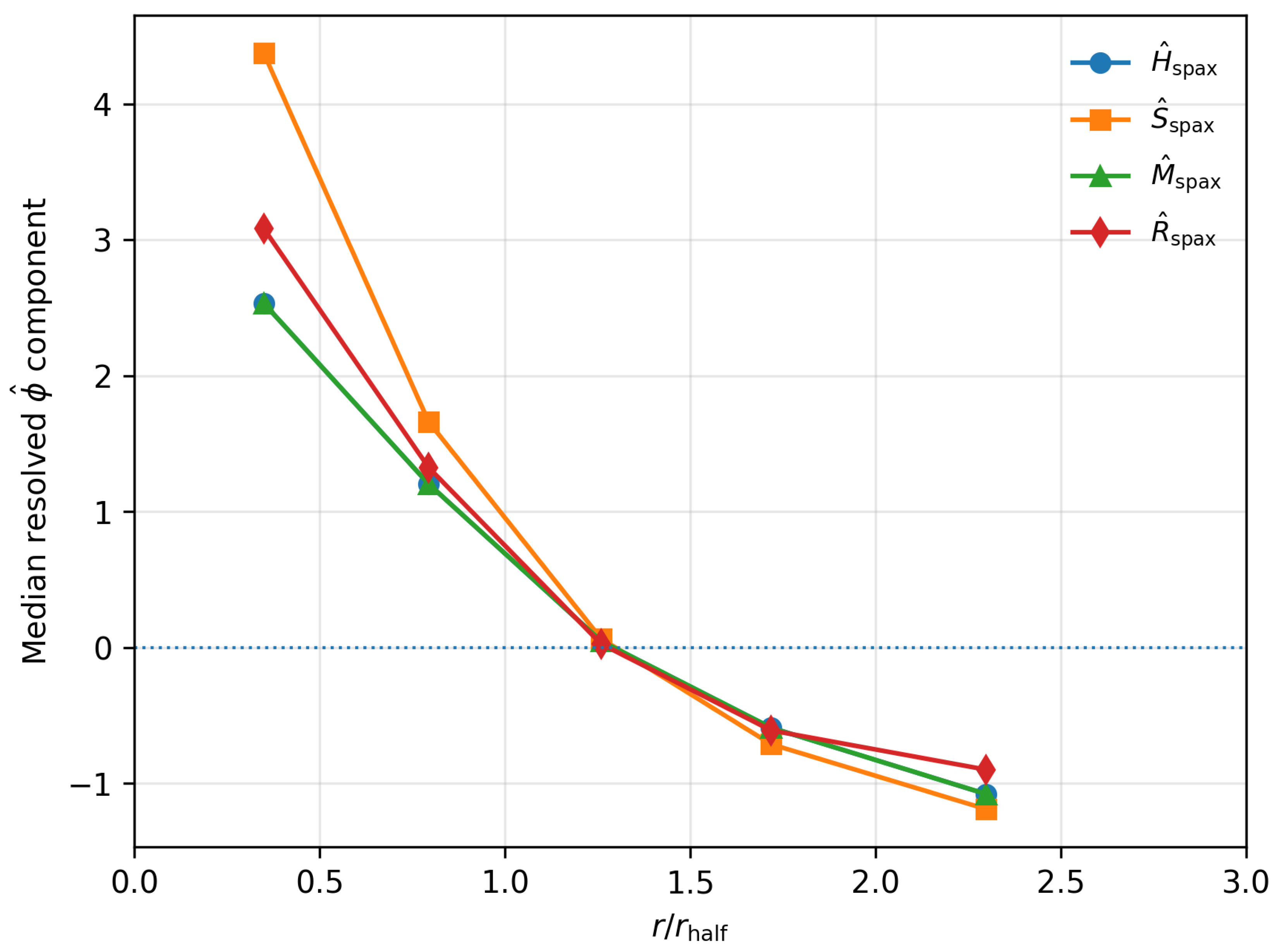
The stacked sample was then binned in radius using

$$r/r_{\mathrm{half}}\in [0.0,0.5],[0.5,1.0],[1.0,1.5],[1.5,2.0],[2.0,3.0],$$

and, in each bin, the median radius and median resolved proxies were measured. Table 1 summarises the result. The innermost bin ($0.0\le r/r_{\mathrm{half}}<0.5$, $N_{\mathrm{spax}}=3197$) has a median radius $r_{\mathrm{med}}\simeq 0.35r_{\mathrm{half}}$ and very high median stability, ${\widehat{S}}_{\mathrm{spax},\mathrm{med}}\simeq 4.38$, together with high mass and regeneration proxies $({\widehat{H}}_{\mathrm{spax},\mathrm{med}}\simeq 2.53,{\widehat{M}}_{\mathrm{spax},\mathrm{med}}\simeq 2.53,{\widehat{R}}_{\mathrm{spax},\mathrm{med}}\simeq 3.09)$. Moving outwards, all four components decline monotonically: by $r/r_{\mathrm{half}}\in [1.0,1.5]$ the medians are close to zero and in the outskirts ($2.0\le r/r_{\mathrm{half}}<3.0$) the medians are negative, with ${\widehat{S}}_{\mathrm{spax},\mathrm{med}}\simeq -1.19$ and ${\widehat{H}}_{\mathrm{spax},\mathrm{med}}\simeq -1.08$.

In other words, the stacked MaNGA spaxels show a clean radial “homeostatic gradient”: inner regions behave like resolved adults in $\widehat{\varphi }$-space (high stability, high memory and high regeneration, all measured relative to the galaxy-wide spaxel distribution), while outer regions behave more like resolved infants (low stability, low memory and low regeneration). The structural gate that separated infant and adult galaxies in the global analysis reappears here as a smooth radial transition inside individual galaxies, with the sign change in the resolved medians occurring around $r\sim r_{\mathrm{half}}$.

Table 1. Stacked MaNGA radial summary for the resolved $\widehat{\varphi }$ proxies. Columns list the radial bin in units of $r_{\mathrm{half}}$, the number of spaxels, the median radius, and the median resolved components $({\widehat{H}}_{\mathrm{spax}},{\widehat{S}}_{\mathrm{spax}},{\widehat{M}}_{\mathrm{spax}},{\widehat{R}}_{\mathrm{spax}})$.

Bin	${\mathit{N}}_{\mathbf{spax}}$	${\mathit{r}}_{\mathbf{med}}$	${\widehat{\mathit{H}}}_{\mathbf{med}}$	${\widehat{\mathit{S}}}_{\mathbf{med}}$	${\widehat{\mathit{M}}}_{\mathbf{med}}$	${\widehat{\mathit{R}}}_{\mathbf{med}}$
0.0–0.5	3197	0.35	2.53	4.38	2.53	3.09
0.5–1.0	8446	0.79	1.20	1.66	1.20	1.33
1.0–1.5	11390	1.26	0.05	0.07	0.05	0.03
1.5–2.0	8906	1.72	-0.59	-0.71	-0.59	-0.61
2.0–3.0	6501	2.30	-1.08	-1.19	-1.08	-0.90

Table 1. Stacked MaNGA radial summary for the resolved $\widehat{\varphi }$ proxies. Columns list the radial bin in units of $r_{\mathrm{half}}$, the number of spaxels, the median radius, and the median resolved components $({\widehat{H}}_{\mathrm{spax}},{\widehat{S}}_{\mathrm{spax}},{\widehat{M}}_{\mathrm{spax}},{\widehat{R}}_{\mathrm{spax}})$.

Bin	${\mathit{N}}_{\mathbf{spax}}$	${\mathit{r}}_{\mathbf{med}}$	${\widehat{\mathit{H}}}_{\mathbf{med}}$	${\widehat{\mathit{S}}}_{\mathbf{med}}$	${\widehat{\mathit{M}}}_{\mathbf{med}}$	${\widehat{\mathit{R}}}_{\mathbf{med}}$
0.0–0.5	3197	0.35	2.53	4.38	2.53	3.09
0.5–1.0	8446	0.79	1.20	1.66	1.20	1.33
1.0–1.5	11390	1.26	0.05	0.07	0.05	0.03
1.5–2.0	8906	1.72	-0.59	-0.71	-0.59	-0.61
2.0–3.0	6501	2.30	-1.08	-1.19	-1.08	-0.90

Figure 1. Stacked radial behaviour of the resolved $\widehat{\varphi }$ proxies in the MaNGA sample. Curves show the median ${\widehat{H}}_{\mathrm{spax}}$, ${\widehat{S}}_{\mathrm{spax}}$, ${\widehat{M}}_{\mathrm{spax}}$, and ${\widehat{R}}_{\mathrm{spax}}$ as a function of $r/r_{\mathrm{half}}$ for all 50 galaxies combined. Inner regions ($r\lesssim 0.5r_{\mathrm{half}}$) occupy a high-stability, high-memory, high-regeneration state, while outer regions ($r\gtrsim 2r_{\mathrm{half}}$) lie in a low-stability, low-memory, low-regeneration state. The zero-crossing of the medians near $r\sim r_{\mathrm{half}}$ marks a resolved version of the infant–adult transition seen in the global $\widehat{\varphi }$ analysis.

Figure 1. Stacked radial behaviour of the resolved $\widehat{\varphi }$ proxies in the MaNGA sample. Curves show the median ${\widehat{H}}_{\mathrm{spax}}$, ${\widehat{S}}_{\mathrm{spax}}$, ${\widehat{M}}_{\mathrm{spax}}$, and ${\widehat{R}}_{\mathrm{spax}}$ as a function of $r/r_{\mathrm{half}}$ for all 50 galaxies combined. Inner regions ($r\lesssim 0.5r_{\mathrm{half}}$) occupy a high-stability, high-memory, high-regeneration state, while outer regions ($r\gtrsim 2r_{\mathrm{half}}$) lie in a low-stability, low-memory, low-regeneration state. The zero-crossing of the medians near $r\sim r_{\mathrm{half}}$ marks a resolved version of the infant–adult transition seen in the global $\widehat{\varphi }$ analysis.

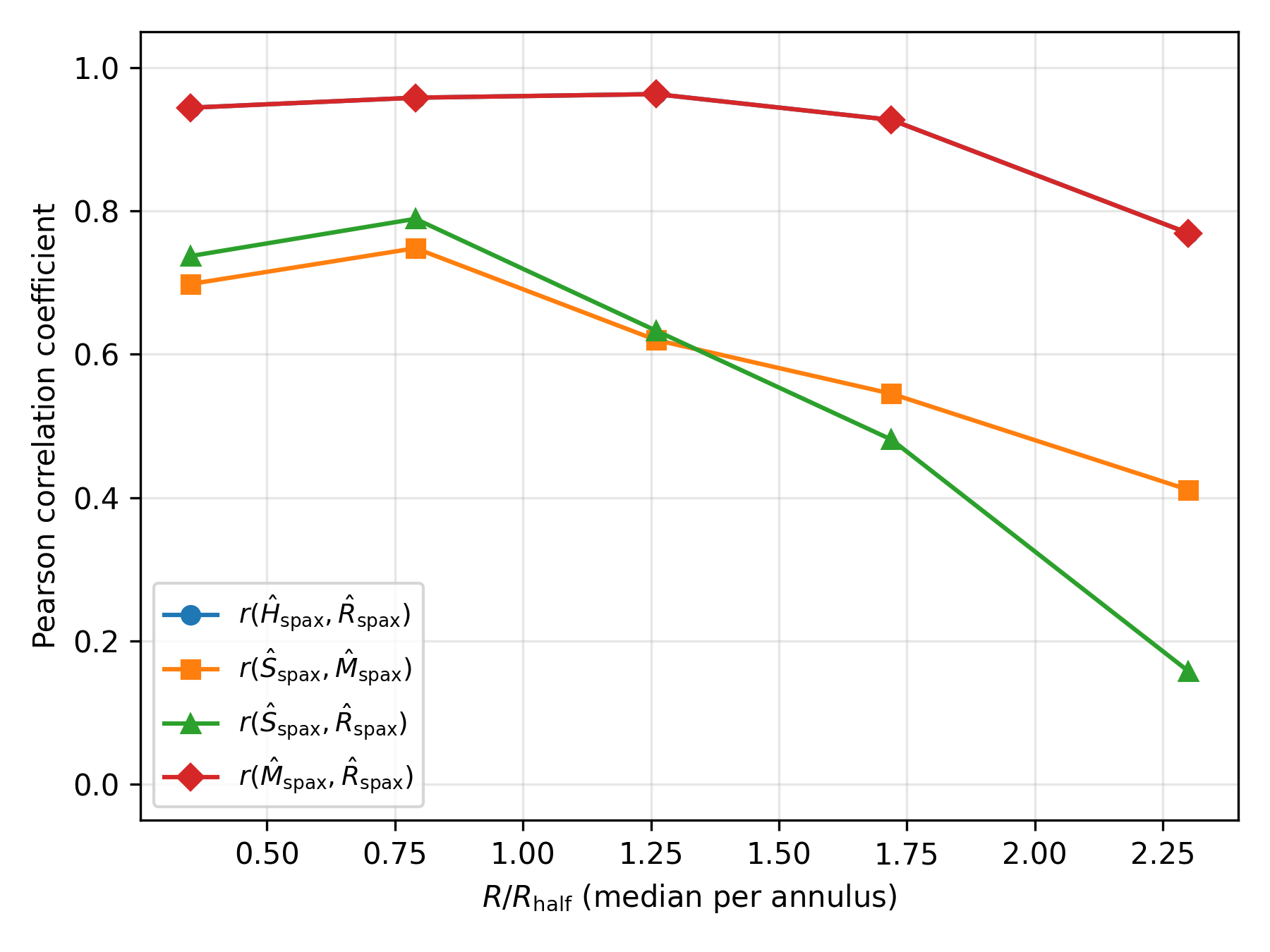
5.2. Radial Coupling of Resolved Homeostatic Components

To test whether the resolved $\widehat{\varphi }$ trends are driven purely by radius, or whether the homeostatic components remain coupled at fixed radius, Pearson correlations were measured between the spaxel-level proxies within the same five annuli in $r/r_{\mathrm{half}}$. The sample of $N=38,440$ spaxels was split and correlations between $({\widehat{H}}_{\mathrm{spax}},{\widehat{S}}_{\mathrm{spax}},{\widehat{M}}_{\mathrm{spax}},{\widehat{R}}_{\mathrm{spax}})$ were computed separately in each bin. The results are summarised in Table 2.

By construction, the energy- and memory-like components are tightly locked ($r_{HM}=1.00$ in all annuli), but the regeneration proxy ${\widehat{R}}_{\mathrm{spax}}$ also tracks them closely inside $\sim 1.5r_{\mathrm{half}}$ ($r_{HR}\simeq r_{MR}\approx 0.94$–$0.96$), only declining to $r_{HR}\simeq 0.77$ in the outermost bin. The stability component ${\widehat{S}}_{\mathrm{spax}}$ remains moderately correlated with both ${\widehat{M}}_{\mathrm{spax}}$ and ${\widehat{R}}_{\mathrm{spax}}$ at small radii ($r_{SM}\approx 0.7$, $r_{SR}\approx 0.7$), but its coupling to regeneration fades in the outskirts ($r_{SR}\simeq 0.16$ for $2.0<r/r_{\mathrm{half}}<3.0$). The inner regions therefore behave like tightly bound “adult” engines with strongly coupled energy, memory and regeneration, while the outskirts are more weakly organised: regeneration remains linked to the global memory budget, but decouples from local structural stability.

Table 2. Radial coupling of resolved homeostatic components in the MaNGA sample. Columns list the number of spaxels $N_{\mathrm{spax}}$, the median radius $r_{\mathrm{med}}$ (in units of $r_{\mathrm{half}}$), and Pearson correlations between spaxel-level components in each radial bin.

Radial bin	${\mathit{N}}_{\mathbf{spax}}$	${\mathit{r}}_{\mathbf{med}}$	${\mathit{r}}_{\mathbf{HM}}$	${\mathit{r}}_{\mathbf{HR}}$	${\mathit{r}}_{\mathbf{SM}}$	${\mathit{r}}_{\mathbf{SR}}$	${\mathit{r}}_{\mathbf{MR}}$
0.0–0.5	3 197	0.35	1.00	0.94	0.70	0.74	0.94
0.5–1.0	8 446	0.79	1.00	0.96	0.75	0.79	0.96
1.0–1.5	11 390	1.26	1.00	0.96	0.62	0.63	0.96
1.5–2.0	8 906	1.72	1.00	0.93	0.55	0.48	0.93
2.0–3.0	6 501	2.30	1.00	0.77	0.41	0.16	0.77

Table 2. Radial coupling of resolved homeostatic components in the MaNGA sample. Columns list the number of spaxels $N_{\mathrm{spax}}$, the median radius $r_{\mathrm{med}}$ (in units of $r_{\mathrm{half}}$), and Pearson correlations between spaxel-level components in each radial bin.

Radial bin	${\mathit{N}}_{\mathbf{spax}}$	${\mathit{r}}_{\mathbf{med}}$	${\mathit{r}}_{\mathbf{HM}}$	${\mathit{r}}_{\mathbf{HR}}$	${\mathit{r}}_{\mathbf{SM}}$	${\mathit{r}}_{\mathbf{SR}}$	${\mathit{r}}_{\mathbf{MR}}$
0.0–0.5	3 197	0.35	1.00	0.94	0.70	0.74	0.94
0.5–1.0	8 446	0.79	1.00	0.96	0.75	0.79	0.96
1.0–1.5	11 390	1.26	1.00	0.96	0.62	0.63	0.96
1.5–2.0	8 906	1.72	1.00	0.93	0.55	0.48	0.93
2.0–3.0	6 501	2.30	1.00	0.77	0.41	0.16	0.77

5.3. Robustness to S/N and Radial Cuts

The resolved profiles in Figure 1 are based on a fiducial MaNGA stack with $\mathrm{S}/{\mathrm{N}}_{\mathrm{H}\alpha }\ge 3$, continuum $\mathrm{S}/\mathrm{N}\ge 5$, and radii up to $3R_{\mathrm{half}}$. To test whether the inner high and outer low pattern in the homeostatic proxies is driven by low-quality spaxels or by the faint outskirts, the full pipeline was rerun under two alternative selections.

Variant 1 (stricter S/N) uses $\mathrm{S}/{\mathrm{N}}_{\mathrm{H}\alpha }\ge 5$ and continuum $\mathrm{S}/\mathrm{N}\ge 7$ at the same radial range $0\le r/R_{\mathrm{half}}\le 3$. This reduces the usable sample from $N_{\mathrm{spax}}=38,440$ to $N_{\mathrm{spax}}=30,519$ but leaves the radial structure intact. The inner annulus still shows large positive medians in the energy and regeneration coordinates, while the $1.5$–$2.0R_{\mathrm{half}}$ band remains negative.

Variant 2 (conservative radial cut) keeps the fiducial S/N selection but limits the analysis to $0\le r/R_{\mathrm{half}}\le 2$. This removes the outermost annulus but still retains $N_{\mathrm{spax}}=31,939$ spaxels in $N_{\mathrm{gal}}=50$ galaxies. The inner medians shift only slightly, and the outer band becomes a little more negative. The energy–regeneration coupling again stays high in the centre and declines with radius.

A third variant with both stricter S/N and the $r/R_{\mathrm{half}}\le 2$ cut ($N_{\mathrm{spax}}=26,686$, $N_{\mathrm{gal}}=49$) gives almost identical inner and outer medians and the same pattern of strong inner coupling and weaker outer coupling. The combined effect of the cuts is therefore to change the error bars, not the structure of the signal. Table 3 summarises the key inner and outer statistics for the three main stacks.

Table 3. Robustness of resolved MaNGA homeostasis to S/N and radial cuts. For each stack the table lists the total number of spaxels, together with median energy and regeneration coordinates and their Pearson coupling at inner (0–$0.5R_{\mathrm{half}}$) and outer ($1.5$–$2.0R_{\mathrm{half}}$) radii.

Stack	${\mathit{N}}_{\mathbf{spax}}$	${\widehat{\mathit{H}}}_{\mathbf{med}}^{\mathbf{in}}$	${\widehat{\mathit{H}}}_{\mathbf{med}}^{\mathbf{out}}$	${\widehat{\mathit{R}}}_{\mathbf{med}}^{\mathbf{in}}$	${\widehat{\mathit{R}}}_{\mathbf{med}}^{\mathbf{out}}$	${\mathit{r}}_{\mathbf{HR}}^{\mathbf{in}}$	${\mathit{r}}_{\mathbf{HR}}^{\mathbf{out}}$
Fiducial (S/N 3,5; $r\le 3R_{\mathrm{half}}$)	38 440	2.53	$-0.59$	3.09	$-0.61$	0.94	0.93
Variant 1 (S/N 5,7; $r\le 3R_{\mathrm{half}}$)	30 519	2.59	$-0.64$	3.07	$-0.65$	0.96	0.93
Variant 2 (S/N 3,5; $r\le 2R_{\mathrm{half}}$)	31 939	2.42	$-1.07$	2.85	$-1.00$	0.98	0.91

Table 3. Robustness of resolved MaNGA homeostasis to S/N and radial cuts. For each stack the table lists the total number of spaxels, together with median energy and regeneration coordinates and their Pearson coupling at inner (0–$0.5R_{\mathrm{half}}$) and outer ($1.5$–$2.0R_{\mathrm{half}}$) radii.

Stack	${\mathit{N}}_{\mathbf{spax}}$	${\widehat{\mathit{H}}}_{\mathbf{med}}^{\mathbf{in}}$	${\widehat{\mathit{H}}}_{\mathbf{med}}^{\mathbf{out}}$	${\widehat{\mathit{R}}}_{\mathbf{med}}^{\mathbf{in}}$	${\widehat{\mathit{R}}}_{\mathbf{med}}^{\mathbf{out}}$	${\mathit{r}}_{\mathbf{HR}}^{\mathbf{in}}$	${\mathit{r}}_{\mathbf{HR}}^{\mathbf{out}}$
Fiducial (S/N 3,5; $r\le 3R_{\mathrm{half}}$)	38 440	2.53	$-0.59$	3.09	$-0.61$	0.94	0.93
Variant 1 (S/N 5,7; $r\le 3R_{\mathrm{half}}$)	30 519	2.59	$-0.64$	3.07	$-0.65$	0.96	0.93
Variant 2 (S/N 3,5; $r\le 2R_{\mathrm{half}}$)	31 939	2.42	$-1.07$	2.85	$-1.00$	0.98	0.91

5.4. Variance–Energy Scaling in Resolved Space

The Unknown Other Principle formulation of the homeostatic model predicts that, at fixed global state, the variance of memory- and regeneration-like observables should scale systematically with the effective energy coordinate. To test this in resolved form, the MaNGA spaxel catalogue is re-binned in the local energy proxy ${\widehat{H}}_{\mathrm{spax}}$, using eight equal-occupancy quantile bins over the full $0\le r/R_{\mathrm{half}}\le 3$ sample. In each bin the median ${\widehat{H}}_{\mathrm{spax}}$ and the variances of ${\widehat{M}}_{\mathrm{spax}}$ and ${\widehat{R}}_{\mathrm{spax}}$ are measured.

Table 4 the variance–energy relation for the fiducial sample. The scatter in both the chemical-memory and regeneration coordinates is smallest at intermediate ${\widehat{H}}_{\mathrm{spax}}$ and increases towards the most energetic spaxels, with a pronounced upturn in the highest bin. The behaviour of $\mathrm{Var}\left({\widehat{M}}_{\mathrm{spax}}\right)$ and $\mathrm{Var}\left({\widehat{R}}_{\mathrm{spax}}\right)$ is closely matched, as expected given the construction of the resolved proxies.

Table 4. Variance–energy scaling for resolved MaNGA spaxels in the fiducial sample ($0\le r/R_{\mathrm{half}}\le 3$). Bins are equal-occupancy quantiles in ${\widehat{H}}_{\mathrm{spax}}$; $H_{\mathrm{med}}$ is the median ${\widehat{H}}_{\mathrm{spax}}$ in each bin. Variances are computed for the normalised resolved memory and regeneration coordinates.

${\widehat{\mathit{H}}}_{\mathbf{spax}}$ bin	${\mathit{N}}_{\mathbf{spax}}$	${\mathit{H}}_{\mathbf{med}}$	$\mathbf{Var}\left({\widehat{\mathit{M}}}_{\mathbf{spax}}\right)$	$\mathbf{Var}\left({\widehat{\mathit{R}}}_{\mathbf{spax}}\right)$
$-2.79$–$-1.43$	4805	$-1.72$	0.080	0.321
$-1.43$–$-0.95$	4805	$-1.18$	0.019	0.176
$-0.95$–$-0.48$	4805	$-0.72$	0.019	0.117
$-0.48$–$0.00$	4816	$-0.24$	0.019	0.090
$0.00$–$0.49$	4794	$0.23$	0.021	0.086
$0.49$–$1.06$	4805	$0.76$	0.028	0.111
$1.06$–$1.85$	4805	$1.42$	0.051	0.174
$1.85$–$5.74$	4805	$2.60$	0.588	1.650

Table 4. Variance–energy scaling for resolved MaNGA spaxels in the fiducial sample ($0\le r/R_{\mathrm{half}}\le 3$). Bins are equal-occupancy quantiles in ${\widehat{H}}_{\mathrm{spax}}$; $H_{\mathrm{med}}$ is the median ${\widehat{H}}_{\mathrm{spax}}$ in each bin. Variances are computed for the normalised resolved memory and regeneration coordinates.

${\widehat{\mathit{H}}}_{\mathbf{spax}}$ bin	${\mathit{N}}_{\mathbf{spax}}$	${\mathit{H}}_{\mathbf{med}}$	$\mathbf{Var}\left({\widehat{\mathit{M}}}_{\mathbf{spax}}\right)$	$\mathbf{Var}\left({\widehat{\mathit{R}}}_{\mathbf{spax}}\right)$
$-2.79$–$-1.43$	4805	$-1.72$	0.080	0.321
$-1.43$–$-0.95$	4805	$-1.18$	0.019	0.176
$-0.95$–$-0.48$	4805	$-0.72$	0.019	0.117
$-0.48$–$0.00$	4816	$-0.24$	0.019	0.090
$0.00$–$0.49$	4794	$0.23$	0.021	0.086
$0.49$–$1.06$	4805	$0.76$	0.028	0.111
$1.06$–$1.85$	4805	$1.42$	0.051	0.174
$1.85$–$5.74$	4805	$2.60$	0.588	1.650

Figure 2. Variance–energy scaling for resolved MaNGA spaxels. Points show the logarithm of the variance of the resolved memory and regeneration coordinates as a function of the median local energy proxy ${\widehat{H}}_{\mathrm{spax}}$ in equal-occupancy bins, for the fiducial $0\le r/R_{\mathrm{half}}\le 3$ sample. The scatter in both ${\widehat{M}}_{\mathrm{spax}}$ and ${\widehat{R}}_{\mathrm{spax}}$ is minimised at intermediate energies and rises sharply towards the most energetic spaxels, indicating enhanced local homeostatic excursions in high-$\widehat{H}$ regions.

Figure 2. Variance–energy scaling for resolved MaNGA spaxels. Points show the logarithm of the variance of the resolved memory and regeneration coordinates as a function of the median local energy proxy ${\widehat{H}}_{\mathrm{spax}}$ in equal-occupancy bins, for the fiducial $0\le r/R_{\mathrm{half}}\le 3$ sample. The scatter in both ${\widehat{M}}_{\mathrm{spax}}$ and ${\widehat{R}}_{\mathrm{spax}}$ is minimised at intermediate energies and rises sharply towards the most energetic spaxels, indicating enhanced local homeostatic excursions in high-$\widehat{H}$ regions.

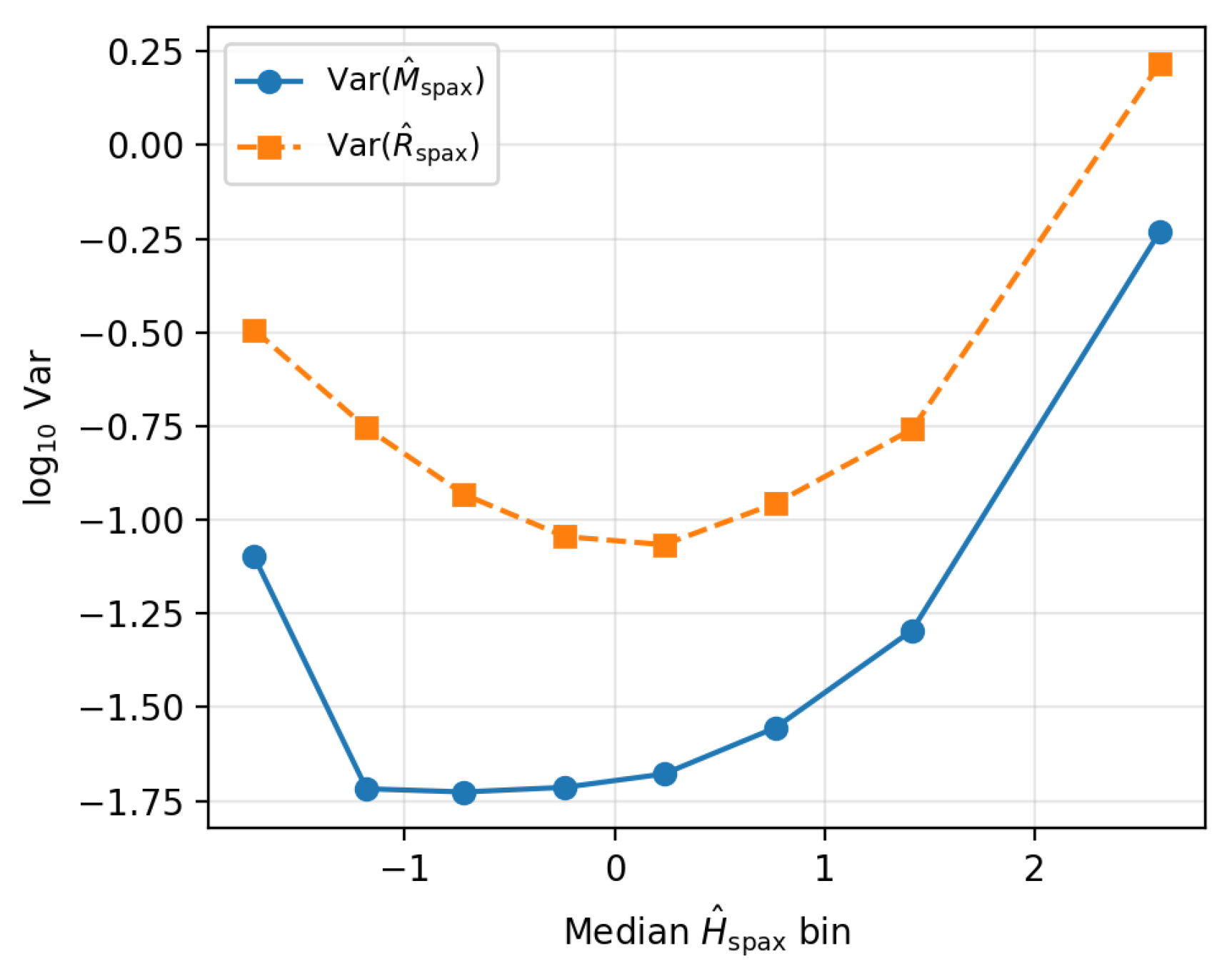
Both $\mathrm{Var}\left({\widehat{M}}_{\mathrm{spax}}\right)$ and $\mathrm{Var}\left({\widehat{R}}_{\mathrm{spax}}\right)$ follow a roughly monotonic increase in ${log}_{10}\mathrm{Var}$ with ${\widehat{H}}_{\mathrm{spax}}$ once the low-$\widehat{H}$ tail is excluded, with a steepening at the highest energies. Repeating the analysis for inner radii only ($r/R_{\mathrm{half}}\le 1$) and for the stricter S/N selection yields qualitatively identical trends, with only small changes in the outermost bin variances.

5.5. Variance–Memory Scaling and Comparison to Simulations

In the original homeostatic tests using IllustrisTNG, the variance–memory scaling was evaluated at the galaxy level: at fixed dynamical state (infant vs. adult), the variance of structural quantities decreased with increasing chemical memory proxy $\widehat{M}$. Fits of the form ${log}_{10}\mathrm{Var}\left(\widehat{S}\right)=a+\gamma {log}_{10}\left|\widehat{M}\right|$ yielded $\gamma <0$ in the TNG infant and adult regimes, i.e. stronger memory meant tighter structural regularity.

For the MaNGA spaxel sample, the same functional form was applied to the resolved proxies. Using stacked spaxels with $0\le r/R_{\mathrm{half}}\le 3$ and the baseline S/N cuts, the variance of the resolved stability proxy ${\widehat{S}}_{\mathrm{spax}}$ increases with $|{\widehat{M}}_{\mathrm{spax}}|$, with a strongly positive slope,

$${log}_{10}\mathrm{Var}\left({\widehat{S}}_{\mathrm{spax}}\right)=a+{\gamma }_{\mathrm{MaNGA}}{log}_{10}\left|{\widehat{M}}_{\mathrm{spax}}\right|,{\gamma }_{\mathrm{MaNGA}}\simeq 0.76.$$

(12)

Restricting to the inner $0\le r/R_{\mathrm{half}}\le 1$ somewhat flattens the relation, but the slope remains positive, while tightening the S/N cuts has negligible impact on the sign. Table 5 summarises these trends.

Table 5. Binned variance–memory statistics for resolved MaNGA spaxels in the fiducial $0\le r/R_{\mathrm{half}}\le 3$ sample. $|{\widehat{M}}_{\mathrm{spax}}{|}_{\mathrm{med}}$ is the median absolute memory in each bin.

$|{\widehat{\mathit{M}}}_{\mathbf{spax}}|$ bin	${\mathit{N}}_{\mathbf{spax}}$	$|{\widehat{\mathit{M}}}_{\mathbf{spax}}{|}_{\mathbf{med}}$	$\mathbf{Var}\left({\widehat{\mathit{H}}}_{\mathbf{spax}}\right)$	$\mathbf{Var}\left({\widehat{\mathit{S}}}_{\mathbf{spax}}\right)$	$\mathbf{Var}\left({\widehat{\mathit{R}}}_{\mathbf{spax}}\right)$
0.00–0.24	4803	0.118	0.019	0.682	0.086
0.24–0.48	4802	0.366	0.137	0.736	0.220
0.48–0.74	4802	0.610	0.377	0.896	0.491
0.74–1.00	4802	0.870	0.752	1.308	0.945
1.00–1.28	4802	1.133	1.264	1.832	1.503
1.28–1.58	4802	1.423	1.950	2.382	2.284
1.58–2.06	4802	1.780	3.216	3.649	3.680
2.06–5.74	4803	2.613	4.363	7.762	6.085

Table 5. Binned variance–memory statistics for resolved MaNGA spaxels in the fiducial $0\le r/R_{\mathrm{half}}\le 3$ sample. $|{\widehat{M}}_{\mathrm{spax}}{|}_{\mathrm{med}}$ is the median absolute memory in each bin.

$|{\widehat{\mathit{M}}}_{\mathbf{spax}}|$ bin	${\mathit{N}}_{\mathbf{spax}}$	$|{\widehat{\mathit{M}}}_{\mathbf{spax}}{|}_{\mathbf{med}}$	$\mathbf{Var}\left({\widehat{\mathit{H}}}_{\mathbf{spax}}\right)$	$\mathbf{Var}\left({\widehat{\mathit{S}}}_{\mathbf{spax}}\right)$	$\mathbf{Var}\left({\widehat{\mathit{R}}}_{\mathbf{spax}}\right)$
0.00–0.24	4803	0.118	0.019	0.682	0.086
0.24–0.48	4802	0.366	0.137	0.736	0.220
0.48–0.74	4802	0.610	0.377	0.896	0.491
0.74–1.00	4802	0.870	0.752	1.308	0.945
1.00–1.28	4802	1.133	1.264	1.832	1.503
1.28–1.58	4802	1.423	1.950	2.382	2.284
1.58–2.06	4802	1.780	3.216	3.649	3.680
2.06–5.74	4803	2.613	4.363	7.762	6.085

Figure 3. Variance–memory scaling for resolved MaNGA spaxels in the fiducial $0\le r/R_{\mathrm{half}}\le 3$ sample. Points show binned medians in $|{\widehat{M}}_{\mathrm{spax}}|$ and ${log}_{10}\mathrm{Var}\left({\widehat{S}}_{\mathrm{spax}}\right)$; the line shows the best–fitting power law with slope ${\gamma }_{\mathrm{MaNGA}}=0.76$. Structural variance increases with the amplitude of the local memory proxy, in contrast to the negative variance–memory slope measured in the TNG boxes.

Figure 3. Variance–memory scaling for resolved MaNGA spaxels in the fiducial $0\le r/R_{\mathrm{half}}\le 3$ sample. Points show binned medians in $|{\widehat{M}}_{\mathrm{spax}}|$ and ${log}_{10}\mathrm{Var}\left({\widehat{S}}_{\mathrm{spax}}\right)$; the line shows the best–fitting power law with slope ${\gamma }_{\mathrm{MaNGA}}=0.76$. Structural variance increases with the amplitude of the local memory proxy, in contrast to the negative variance–memory slope measured in the TNG boxes.

The sign difference between the simulated galaxy-level behaviour (${\gamma }_{\mathrm{TNG}}<0$) and the resolved MaNGA result (${\gamma }_{\mathrm{MaNGA}}>0$) suggests that the two measurements probe different regimes of the same underlying dynamics. In the global TNG tests, the classification explicitly selects galaxies that have already passed through the stability gate and evolved into quasi-regular adult systems: in that regime, memory compresses variance. In the MaNGA case, the analysis weights individual spaxels by area and H$\alpha$ S/N, and is therefore dominated by actively driven regions within otherwise regulated galaxies. In such patches, the same feedback and inflow events that increase $|{\widehat{M}}_{\mathrm{spax}}|$ also introduce local structural disorder, leading to a branch where memory and variance grow together.

A dedicated set of mock IFU experiments is therefore a natural next step: three-dimensional simulated galaxies can be projected to MaNGA-like cubes, convolved with a realistic PSF, and passed through the same resolved $\widehat{\varphi }$ pipeline as the real MaNGA sample. In parallel, resolved TNG and EAGLE analyses that treat simulation cells as “spaxels” can be used to measure variance–memory scaling at fixed relaxation state. These tests will allow a direct separation between genuine physical differences and observational effects, and clarify how the homeostatic branch (variance suppression) and the driven branch (variance amplification) emerge from the same underlying homeostatic potential.

6. Discussion

6.1. Inner Processors and Outer Reservoirs

The stacked radial profiles and coupling diagnostics point to a simple picture. Inner regions of MaNGA galaxies behave like resolved homeostatic processors: they occupy a high-stability, high-memory, high-regeneration state and exhibit tight coupling between energy, memory and regeneration. The outer regions behave more like reservoirs: they are lower in all four components, structurally less settled, and show weaker coupling between stability and regeneration.

This inside–out organisation is consistent with the global infant/adult framework. Globally adult galaxies are those in which a large fraction of the stellar mass and star formation resides in the inner, adult-like regime. Globally infant galaxies are those dominated by extended, structurally plastic regions. The resolved analysis shows that most systems mix both behaviours in radius; the global classification is a weighted average of resolved states. In other words, the MaNGA stack appears to be dominated by a driven branch in which active regions inside otherwise regulated galaxies overshoot their structural equilibrium, whereas the TNG global tests emphasise a homeostatic branch in which long–term memory compresses structural variance.

6.2. Resolved Homeostasis and Environmental Influence

The environment analysis at the galaxy level shows that environment acts as a strong modulator of the memory budget before the stability gate is crossed, but mainly tunes residual variance once galaxies have internalised their history into a stable configuration. The resolved MaNGA results suggest where this modulation is applied.

In an inside–out picture, environment and inflow histories will imprint most strongly on the outer, infant-like disc, where stability is low and regeneration is easily perturbed. The central, adult-like regions are more insulated: they still respond to external conditions, but much of their memory budget is carried by their own internal configuration. Satellite galaxies with stripped outskirts but intact cores provide one obvious playground for this picture: the resolved homeostatic framework could be used to quantify how much of the environmental impact is absorbed in the outer reservoirs versus the inner processors.

6.3. Systematics, Limitations and Future Work

Several caveats apply. The MaNGA sample is small and not statistically complete. The resolved proxies are deliberately simple, relying on S/N and H$\alpha$ flux as crude tracers of mass and regeneration. Beam smearing, metallicity calibration uncertainties, limited radial coverage, and S/N cuts all affect the outskirts. No explicit separation of star-forming, AGN and shock-excited regions has been implemented.

These limitations point directly to extensions. The same resolved framework can be combined with full MaNGA DAP maps, applied to larger IFU surveys such as SAMI and CALIFA, and implemented in mock IFUs from simulations. Time evolution can be brought in via age gradients and multi-epoch snapshots in simulations. On the theoretical side, the variance–memory tension between MaNGA and TNG can be turned into a falsifiable target: either mock IFUs will reveal that the apparent sign difference is an observational selection effect, or the simulations will have to be recalibrated to produce the driven branch observed in the real resolved data.

7. Conclusions

This paper has used MaNGA integral-field spectroscopy to test the homeostatic potential framework at the spaxel level. The main conclusions are:

1.

Stacked MaNGA spaxels show a clean radial homeostatic gradient: inner regions sit in a high-stability, high-memory, high-regeneration state, while outer regions are depleted in all four components, with the median resolved components crossing zero near $r\sim R_{\mathrm{half}}$.

2.

The regeneration proxy remains tightly coupled to both energy and memory at all radii, but its coupling to the stability coordinate weakens in the outskirts, indicating a gradually loosening but still coherent resolved homeostatic network.

3.

The radial trends and coupling patterns are robust to stricter S/N cuts and to conservative radial selections, changing the error bars but not the structure of the signal.

4.

Variance–energy and variance–memory scalings reveal a driven branch in which regions with stronger local chemical memory also host larger structural excursions, in contrast to the variance suppression seen in global tests on simulations.

In combination with the global SDSS analysis, which measures the double flip in single–fibre proxies, the MaNGA results show that the same homeostatic transition appears in radius inside galaxies: inner regions behave like compact adult processors, while outer discs act as extended reservoirs. In this sense, the stability gate is a resolved property inside galaxies, not just a global label. Galaxies mix inner processors and outer reservoirs in radius, and the homeostatic framework provides a compact way to track how energy, stability, memory and regeneration organise themselves across those scales. Mock IFUs and larger survey samples will allow the same logic to be pushed to the point where mismatches between simulations and data can be treated as explicit homeostatic falsifiers.

Appendix B.1. Summary of Sample Variants

To test the robustness of the resolved homeostatic pattern, a repeat of the full pipeline under stricter S/N cuts and a more conservative radial range, is implemented. Table A6 summarises the four spaxel sets used in the main text and in this Appendix.

Table A6. MaNGA resolved $\widehat{\varphi }$ samples used for robustness tests. All variants use the same 50-galaxy parent selection; quoted $N_{\mathrm{spax}}$ values refer to spaxels that pass the stated S/N and radius cuts and enter the construction of $({\widehat{H}}_{\mathrm{spax}},{\widehat{S}}_{\mathrm{spax}},{\widehat{M}}_{\mathrm{spax}},{\widehat{R}}_{\mathrm{spax}})$.

Variant	S/N cuts (H$\mathit{\alpha }$, cont)	${\mathit{r}}_{max}/{\mathit{R}}_{\mathbf{half}}$	${\mathit{N}}_{\mathbf{spax}}$
Baseline	(3, 5)	3.0	38 440
High S/N	(5, 7)	3.0	30 519
Inner only	(3, 5)	2.0	31 939
High S/N + inner only	(5, 7)	2.0	26 686

Table A6. MaNGA resolved $\widehat{\varphi }$ samples used for robustness tests. All variants use the same 50-galaxy parent selection; quoted $N_{\mathrm{spax}}$ values refer to spaxels that pass the stated S/N and radius cuts and enter the construction of $({\widehat{H}}_{\mathrm{spax}},{\widehat{S}}_{\mathrm{spax}},{\widehat{M}}_{\mathrm{spax}},{\widehat{R}}_{\mathrm{spax}})$.

Variant	S/N cuts (H$\mathit{\alpha }$, cont)	${\mathit{r}}_{max}/{\mathit{R}}_{\mathbf{half}}$	${\mathit{N}}_{\mathbf{spax}}$
Baseline	(3, 5)	3.0	38 440
High S/N	(5, 7)	3.0	30 519
Inner only	(3, 5)	2.0	31 939
High S/N + inner only	(5, 7)	2.0	26 686

Across all variants, the qualitative behaviour of the stacked radial profiles is unchanged. For the baseline sample, the median resolved components show a clear inner–high / outer–low pattern: inside $0.5R_{\mathrm{half}}$ the paper finds ${\widehat{H}}_{\mathrm{spax}}\sim 2.5$ and ${\widehat{S}}_{\mathrm{spax}}\sim 4.4$, while beyond $2R_{\mathrm{half}}$ they drop to ${\widehat{H}}_{\mathrm{spax}}\sim -1.1$ and ${\widehat{S}}_{\mathrm{spax}}\sim -1.2$. The resolved memory and regeneration components follow the same trend. Tightening the S/N thresholds to $(5,7)$ or restricting to $r/R_{\mathrm{half}}\le 2$ changes the amplitudes by at most a few tenths of a dex but leaves the ordering (inner > intermediate > outer) intact. The radial coupling between components remains strong: the Pearson correlation $r({\widehat{H}}_{\mathrm{spax}},{\widehat{R}}_{\mathrm{spax}})$ and $r({\widehat{M}}_{\mathrm{spax}},{\widehat{R}}_{\mathrm{spax}})$ stays positive in every annulus and declines smoothly with radius in all four variants, never flipping sign. In other words, the existence and radial weakening of resolved homeostasis does not rely on a particular choice of S/N or radius cut.

Appendix B.2. Variance–Memory Scaling in Resolved Space

A key result of the previous global analyses is a variance–memory scaling: the structural variance changes systematically with the absolute memory component, with global TNG tests favouring variance suppression ($\gamma <0$) as $|\widehat{M}|$ increases.

For each resolved sample, the paper bins spaxels by $|{\widehat{M}}_{\mathrm{spax}}|$, compute the variance of each homeostatic component in each bin, and fit a power law of the form

$${log}_{10}\mathrm{Var}\left({\widehat{S}}_{\mathrm{spax}}\right)=a+\gamma {log}_{10}\left|{\widehat{M}}_{\mathrm{spax}}\right|.$$

For the baseline 0–3 $R_{\mathrm{half}}$ sample the paper finds $\gamma \simeq 0.76$ with a tight correlation ($r\simeq 0.88$). Restricting to the inner disc (0–1 $R_{\mathrm{half}}$) gives a slightly shallower slope, $\gamma \simeq 0.57$, while the high-S/N 0–3 $R_{\mathrm{half}}$ variant yields $\gamma \simeq 0.77$ ($r\simeq 0.91$). Within uncertainties, the exponent lies in the range $\gamma \approx 0.6$–0.8 across all three cases.

This resolved variance–memory scaling shows that the dispersion in the local stability coordinate is not arbitrary: regions with large $|{\widehat{M}}_{\mathrm{spax}}|$ also exhibit larger scatter in ${\widehat{S}}_{\mathrm{spax}}$. In the language of homeostasis, strong local “memory” is accompanied by a broader spread of structural states, consistent with the idea that memory both stabilises and stretches the range of accessible configurations. The fact that this scaling survives stricter S/N cuts and an inner radius restriction indicates that it is not a boundary artefact or a tail effect in a handful of noisy spaxels, but a generic feature of the resolved homeostatic field.

References

- Peng, Y.; Lilly, S.J.; Kovac, K.; et al. Mass and Environment as Drivers of Galaxy Evolution in SDSS and zCOSMOS. Astrophysical Journal 2010, 721, 193–221, [1003.4747. [Google Scholar] [CrossRef]
- Bundy, K.; Bershady, M.A.; Law, D.R.; Yan, R.; Drory, N.; MacDonald, N.; Wake, D.A.; Cherinka, B.; Sánchez-Gallego, J.R.; Weijmans, A.M.; et al. Overview of the SDSS-IV MaNGA Survey: Mapping Nearby Galaxies at Apache Point Observatory. The Astrophysical Journal 2015, 798(7), 1412.1482. [Google Scholar] [CrossRef]
- Atalebe, S. From Processors to Reservoirs: The Stability Gate and the Homeostatic Double Flip in Galaxy Evolution. Preprints 2026, 1–10. [Google Scholar] [CrossRef]
- Atalebe, S. Environment as a Modulator of Homeostatic Potential in Galaxy Evolution. In preprints.org; Preprint, 2026. [Google Scholar]
- Cherinka, B.; Andrews, B.H.; Sánchez-Gallego, J.R. Marvin: A Tool Kit for Streamlined Access and Visualization of the SDSS-IV MaNGA Data Set. The Astronomical Journal 2019, 158(74), 1812.03833. [Google Scholar] [CrossRef]
Disclaimer/Publisher’s Note: The statements, opinions and data contained in all publications are solely those of the individual author(s) and contributor(s) and not of MDPI and/or the editor(s). MDPI and/or the editor(s) disclaim responsibility for any injury to people or property resulting from any ideas, methods, instructions or products referred to in the content. |
© 2026 by the authors. Licensee MDPI, Basel, Switzerland. This article is an open access article distributed under the terms and conditions of the Creative Commons Attribution (CC BY) license (http://creativecommons.org/licenses/by/4.0/).
Copyright: This open access article is published under a Creative Commons CC BY 4.0 license, which permit the free download, distribution, and reuse, provided that the author and preprint are cited in any reuse.