
Submitted:
16 January 2026
Posted:
22 January 2026
You are already at the latest version
Abstract
An innovative pin-fin integrated thermoelectric device (iTED) is numerically modeled to quantify the effect of thermal flow conditions, namely inlet temperature (\( T_{\textrm{in}} \)) and Reynolds number (Re), as well as electrical load resistance (\( R_{\textrm{load}} \)), on the thermal-electric-fluid coupled performance. Quantification of the simultaneous thermal-fluid-electric behavior of the iTED was pursued through the implementation of an explicitly-coupled solution algorithm developed in ANSYS Fluent's User Defined Scalar (UDS) environment. The effects of \( T_{\textrm{in}} \), Re, and \( R_{\textrm{load}} \), which were varied between 350 and 650 K, 3,000 and 15,000, and 0.01 and \( 10^{6} \% \) of the internal device resistance (\( R_{\textrm{int}} \)), respectively, on the open-circuit voltage, current, power output (\( \dot{W} \)), heat input, pumping power, device thermal conversion efficiency (\( \eta \)), and dimensionless performance index (\( \zeta \)), were evaluated for a fixed cold-side temperature of 300 K. The performance of the iTED was then compared to that of a conventional TEG. At a \( T_{\textrm{in}} \) of 650 K, the iTED achieved a maximum \( \dot{W} \) of 23.9 W when \( R_{\textrm{load}}=R_{\textrm{int}} \) at a Re of 15,000, a maximum \( \eta \) of \( 8.1\% \) when \( R_{\textrm{load}} \) < \( R_{\textrm{int}} \) at a Re of 10,000, and a maximum \( \zeta \) of 7.8 at a Re of 3,000. In comparison, the conventional device achieved a \( \dot{W} \) of 5.2 W, an \( \eta \) of 2.9%, and a \( \zeta \) of 1.6 at the same \( T_{\textrm{in}} \) and Re of 15,000, 6,000, and 3,000, respectively. The proposed multiphysics numerical modeling illustrates marked improvements via device restructuring.
Keywords:
computational fluid dynamics (CFD)
; fluid-thermal-electric coupling
; integrated thermoelectric device (iTED)
; multiphysics modeling
; thermoelectric generator (TEG)
1. Introduction
Due to a growing environmental consciousness, efforts are being made to increase the efficiency of processes and cycles while simultaneously reducing greenhouse gas emissions. Thermoelectric devices (TEDs) are an apposite technology for waste heat recovery applications which can mitigate the adverse effects of fossil-fuel-based power generation and transportation. These two aforementioned sectors are primarily responsible for the vast majority of rejected thermal energy, which is a byproduct of combustion of fossil fuels, in the United States [1]. Thermoelectric generators (TEGs), a subset of TEDs, are solid-state, direct energy conversion devices that capitalize on the Seebeck effect to convert a thermal gradient into an electric potential [2]. These devices are comprised of periodic n- and p-type semiconductors connected electrically in series via electrically conductive bridges. The junctions are then exposed to a thermal gradient which enables the flow of electrons. The materials within the TEG have a large Seebeck coefficient (), on the order of tenths of mV K−1, high electric conductivity (), and low thermal conductivity (), as to maintain a large temperature gradient across the device [3,4]. The performance of the material, which subsequently dictates the device performance, is quantified by the figure of merit .
The modified dimensionless figure of merit represents the performance of a given thermoelectric material. The material performance is evaluated at the average temperature between the cold and hot junctions. A more simplified approach evaluates the material’s performance at the absolute temperature T, yielding , the value most commonly reported in the literature. During the 1950’s, semiconductors with higher thermoelectric performance (0.8) were developed, which aided in the development of devices with more favorable performance [5,6]. The introduction of nanostructures in the 1990’s allowed for the development of materials with higher figures of merit, up to 1.7 [7]. Recently, materials have been shown to achieve a of 2.1, making TEGs more attractive for waste heat recovery applications [8]. Historically, bismuth telluride is shown to be the optimal material for use at low temperatures, around room temperature [9,10,11]. At higher temperatures, i.e. 500-650 °C, lead tellurides have proven effective [9,12]. Skutterudites have also exhibited high figures of merit when operating at high temperatures [13]. Improvement in material efficiency is evidently vital for demonstrating the efficacy of TEGs for waste heat recovery applications. However, this is not the only consideration as the design of the module proves comparably relevant.
The application of conventional TEGs to automotive waste heat recovery has been extensively studied; noteworthy and relevant works will be presented in the following. Kumar et al. developed numerical models to quantify the performance of conventional TEGs applied to the exhaust system of a passenger vehicle, including provisions for the thermal-hydraulic performance of the heat exchanger system and electrical performance of the module. Their results indicated that increasing both the exhaust temperature and flow rates leads to an increase in electrical power generation; however, said increase is limited to the heat transfer coefficient that implicitly develops. The maximum power output obtained was 552 W with a thermoelectric conversion efficiency of 5.50% and a system efficiency of 3.3% [14]. Further studies by Kumar et al. indicated that heat exchanger design was vital to favorable system performance. By constructing a heat exchanger that allowed for the transverse flow of exhaust gas across the modules, a maximum power output with a lesser pressure drop was yielded, thus marginally increasing system efficiency [15]. Similarly, Sun et al. developed a mathematical model to quantify the performance of a two-stage TEG system applied to an internal combustion engine. Aligned with the findings of Kumar et al., they found that the TEG performance was directly dependent upon the waste heat temperature and flow rate, indicating that system performance is contingent upon the thermal-hydraulic performance of the heat exchanger [16].
To facilitate waste heat recovery in automotive applications, efforts have been made to more effectively capture and convert the waste heat. The incorporation of heat pipes into a TEG waste heat recovery system has been studied. Heat pipes have the potential to reduce the thermal resistance between the exhaust gas and the TEG, effectively increasing the temperature difference across the TEG as well as decreasing the pressure loss in the system [17]. Kim et al. developed an experimental apparatus to investigate the use of TEGs and heat pipes from automotive waste heat recovery and found that a maximum power output of 350 W could be achieved [18]. The use of different metal foams on TEGs has also been investigated [19,20]. Nithyanandam and Mahajan studied a silicon carbide foam and the effect pore density and porosity had on the net power produced by a TEG. They found the maximum net power was nearly 8 times the maximum produced by the same TEG without metal foam [19].
Although conventional TEGs have effectively been shown to convert the thermal energy of exhaust gas into usable electricity, thereby increasing system efficiency, there still exist fundamental deficiencies. Inherent to the conventional TEG design is the presence of ceramic between the hot-side junction and the hot-side heat exchanger, as to provide electrical insulation between the TEG and heat exchanger as well as structural support. The thermal resistance associated with the heat exchanger, but more importantly the ceramic, decreases performance by effectively reducing the temperature difference across the junction [21,22,23]. The thermal greases and adhesives used to make contact between the hot-side junction and ceramic, and the ceramic and heat exchanger, diminish the temperature difference established across the junction, thereby decreasing performance [24]. Efforts have been made to overcome these resistances. Kim et al. constructed and tested a direct contact thermoelectric generator, as well as constructed a numerical model thereof, in which the hot-side heat exchanger of the TEG was removed, and the hot-side ceramic was placed directly in contact with the exhaust flow. They found that increased engine loads and speeds, which contribute to greater quantities of thermal energy at higher temperatures and the evolution of convective heat transfer coefficients, increased TEG performance, achieving upwards of 2% thermal conversion efficiency and 45 W of power output [25]. Although novel, the decreased heat exchanger surface area and lack of features to disturb the formation of a thermal and momentum boundary layer over the TEG surfaces prevents the system from experiencing a large temperature gradient. Ma et al. furthered the notion of the necessity to reduce thermal resistance between heat source and sink by replacing the fins of the heat exchanger with thermoelectric material [26]. The work demonstrated the novel configuration but more importantly identified potential issues with actual implementation, namely the induction of large stresses on the TE material due to large stream-wise temperature variations. When considering coefficients of thermal expansion for the TE material and metallic substrate, and the fact the TE material is bonded to the substrate for a relatively large length (200 mm in this study), delamination or cracking would inevitably occur.
An encouraging solution to overcome the thermal resistance of the ceramic and associated greases as well as increase the hot-side heat transfer while minimizing unnecessary thermally-induced stresses is the integrated thermoelectric device (iTED). This novel design allows for the elimination of the hot-side ceramic and greases by directly incorporating the hot-side heat exchanger into the hot-side interconnector. The exhaust gas flow is directed over the hot-side heat exchanger through a dielectric flow conduit. Through this modification, larger temperature gradients can be maintained across the junctions and larger quantities of heat can be extracted from the waste heat stream. The present study presents a thermal-fluid-electric coupled finite volume model to study the effect of thermal-hydraulic parameters on said innovative design in comparison to a conventional design. The range of operational parameters, namely exhaust gas temperature and flow rate, are reflective of on-road heavy-duty diesel vehicles [27], and serve as an extension to previous analytical [28], numerical [29,30,31,32], and experimental [33] studies into the turbulent flow regime.
2. Materials and Methods
2.1. Integrated Thermoelectric Device Design
The pin-fin iTED is schematically depicted in Figure 1. The pin-fins serve dual purposes. The first is to bridge the hot-sides of the opposing p- and n-type materials forming an electrical connection such that the device operates electrically in series and thermally in parallel, as does a conventional TED. The second is to promote turbulence, specifically, the induction of vortex shedding, to promote high heat transfer coefficients on the down-stream pins, thus augmenting the hot-side junction temperatures and heat input. The pin-fins are constrained by a dielectric flow channel which directs the hot-fluid flow over the heat exchanger bank. Although the iTED operates like a conventional thermoelectric device, the restructured configuration eliminates the hot-side ceramic that is typically used as an electrical insulator between the hot-side heat exchanger and hot-side junctions. Furthermore, there exists no need for the grease otherwise used to minimize thermal contact resistance between said heat exchanger, hot-side ceramic, and hot-side junctions, further diminishing the thermal resistance between the heat source and sink.
To demonstrate the efficacy of the iTED in comparison to a conventional device configuration, a favorable, yet not optimized, heat exchanger configuration was selected. The pin-fin height-to-diameter ratio was set at five, for ratios greater than two have been shown to increase pin heat transfer for relatively low-Reynolds number (Re) flow, i.e. up to a value of 30,000 [34]. Additionally, by staggering the pins as depicted in Figure 2, convective heat transfer increases due to wake turbulence from upstream pins [35,36]. The iTED is comprised of 35 pins configured in ten rows, where the number of pins per row alternates between three and four. To keep the transverse spacing () between pins uniform in each row, corbels, or half-cylinders, were introduced on the walls of the dielectric flow channel for the row containing three pins, as shown in Figure 2.
As shown in Figure 1 and Figure 2, the proposed iTED has a flow-channel width (W) of 31.75 mm and a height of 15.875 mm. The inlet Re is calculated based on the hydraulic diameter of the inlet, as opposed to the pin diameter. The pins and pellets have a diameter (D) of 3.175 mm. The and longitudinal spacing () of the pins is 2.5D and 2D, respectively. Thus, the centerline-to-centerline length (L) of the pin array is 57.15 mm. The thermoelectric pellets and cold-side interconnectors are taken as 1 mm thick. This configuration reflects a device with 35 pin-fins and p-n junctions and 36 cold-side interconnectors. Based on and , the packing density, or area of thermoelectric material per unit area of the device, is 15.7%.
2.2. Finite-Volume Domain Generation
The numeric domain representing the conventional and integrated thermoelectric devices was constructed in ANSYS ICEM (Version 17.2). Hexahedral elements were constructed in a highly orthogonal, conformal manner to create a non-uniform, structured mesh. Within the fluid domain, an inflation layer was constructed on all solid surfaces that interfaced with the fluid domain such that the maximum per the highest Re and inlet temperature () values were globally sub-unity. The solid domains, which are the aluminum pins and interconnectors, and n- and p-type thermoelectric materials, are shown in Figure 3. The coarse mesh for a rod, thermoelectric pellets and interconnector is shown overlaid on the last row of solids. A detailed view of the working fluid domain, complete with insets demonstrating the refinement around the pin-fins, is presented in Figure 4.
2.3. Governing Equations
The concurrent characterization of the thermal-hydraulic behavior of the fluid domain and resultant thermal-electric response within the solid domains of the conventional and integrated thermoelectric devices required a unique iterative solution algorithm. Thus, a thermal-fluid-electric field model was implemented in ANSYS Fluent (Version 17.2) using the C-based UDS environment. The thermal-fluid behavior of the fluid and solid domains was solved for using Fluent’s standard flow and energy solver, respectively, whereas the thermoelectric phenomena within the solid domains were resolved using UDSs. The Joule, Thomson and Peltier heats were calculated based upon the temperature distributions within the solid domains, as obtained by the standard energy solver, and then coupled to the general energy transport equation via volumetric and surface source terms. The three aforementioned source terms were applied to the thermoelectric solid domains, whereas only Joule heating was applied to the non-thermoelectric solid domains. The electric fields, expressly the Seebeck electromotive force (SEMF) and electric potential (EP) were calculated within the UDS and modeled via diffusion equations. The internal electrical resistance was also calculated via a volume-weighted sum of each element’s resistance within each respective domain. This methodology reflects an explicitly-coupled scheme the allows for the simultaneous resolution of the thermal-fluid-electric behavior of the conventional and integrated thermoelectric devices. The pertinent governing equations for the fluid and solid domains, and respective boundary conditions are discussed in the following.
2.3.1. Fluid Domain
The thermal-fluid behavior of the fluid domain was pursued via a finite-volume discretization methodology of the governing continuity, momentum and thermal energy transport equations, which were solved on the aforementioned mesh, which represents the numerical domain. To model the turbulent phenomena present within the specified flow regime, the Reynolds Averaged Navier-Stokes (RANS) continuity, momentum and thermal energy transport equations were employed. Considering the steady flow of a Newtonian fluid, the continuity equation, Equation 1, and momentum equation, Equation 2, are expressed as
The total thermal energy transport equation, due to turbulence, is expressed as Equation 3:
During the process of constructing RANS conservation equations, two closure terms arise within Equations 1 and 2, known as the Reynolds stress tensor and turbulence heat flux. These two terms are a consequence of the turbulent behavior of the fluid, and need to be expressed via an additional set of conservation equations. To such an end, the model was employed to provide the necessary closure.
The application of Equation 2 requires four boundary conditions; one for each component of velocity and one for pressure. Thus, at the inlet of the fluid domain, Re values ranging from 3,000 to 15,000 in increments of 3,000 were applied. At the exit of the fluid domain, a zero-gauge pressure outlet boundary condition was applied. For all interior surfaces of the fluid domain, i.e. all channel walls and fluid-rod interfaces, a no-slip boundary condition was applied. The application of Equation 3 requires two boundary conditions. The first is applied at the inlet, where the fluid inlet temperature was varied between 350 and 650 K, in increments of 50 K. The second thermal boundary condition was applied at the cold-side of the interconnectors, with a constant temperature of 300 K. The fluid-rod interfaces were modeled with a conservative heat flux condition. The aforementioned conditions, which reflect the thermal-hydraulic behavior of heavy-duty diesel powered vehicles, provide 35 unique operational points for the integrated and conventional devices.
2.3.2. Solid Domains
The solid domains, thermoelectric and non-thermoelectric, were each governed by a unique thermal equation. The thermoelectric material domains, i.e. n- and p-type materials, were governed by the thermoelectric general energy equation, Equation 4, which is expressed as
The second and third terms in Equation 4 represent the Joule and Thomson heats, respectively, and were modeled using volumetric source terms. The fourth term represents the Peltier heat, and was modeled as a surface source term. The non-thermoelectric domains, i.e. hot-side heat exchangers and cold-side interconnectors, were governed by the general energy transport equation, Equation 5, such that
Both thermoelectric and non-thermoelectric domains were also governed by the continuity of electric current, Equation 6, expressed as
To simultaneously couple the thermal and electric governing equations, the current density vector used within Equations 4, 5 and 6, was determined by the magnitude of the open-circuit voltage, , and internal resistance, . The , commonly referred to as the Seebeck voltage, is calculated as the summation of the open-circuit voltage potentials of each thermoelectric pellet at their respective interfaces between the pin and interconnectors such that
Then, of the device is calculated as
Therefore, the magnitude of the current density, based upon Equations 7 and 8, which is applied to the outlet terminal, is calculated as
The electric potential is expressed through the non-Ohmic voltage-current relation [37], and was modeled as diffusivity within the UDS environment through the entirety of the thermoelectric and non-thermoelectric solids domains. The Seebeck electromotive force, or the second term in the second expression to follow, was also modeled as a diffusivity within the UDS environment, but only in the thermoelectric domains. Thus, the non-Ohmic voltage-current relation is expressed as:
At the inlet terminal, a zero voltage potential is applied such that
The remaining boundaries of the system are treated as electrically insulated such that
At the interfaces of the hot-side interconnectors, pellets and cold-side interconnectors, the continuity of current density is applied such that
Thus, the current, as well as electric potential, implicitly develop with the solution. As for the thermal boundary conditions, the bottom and top surfaces of the bottom-side and top-side interconnectors are maintained at a constant temperature of 300 K, yielding
The exterior surfaces of the pellets and interconnectors are exposed to ambient convective conditions such that
The ambient fluid temperature is kept constant at 300 K and the convective heat transfer coefficient was kept invariant at 10 W m−2 K−1. The inlet and outlet terminals are assumed adiabatic such that
At the interfaces between the hot-side interconnectors, pellets, and cold-side interconnectors, continuity of temperature and heat flux are imposed, yielding:
The electrical power output is determined from the quotient of I and the sum of the and , where is equal to as to maximize power output, such that
Additionally, is varied between 0.01 and 106% of , and the variation of I, , , , , , and is presented.
The heat removed from the fluid and entering the conventional and integrated thermoelectric devices, , is a function of the mass flow rate, specific heat and the temperature difference between inlet and exit. The mass flow rate is expressed as the inlet cross-sectional flow area times velocity times the density, taken as the integral average evaluated between the inlet and exit temperatures. The specific heat, as reported by [38], is also evaluated as the integral average between the inlet and exit temperatures. Lastly, the temperature difference between the inlet and exit of the fluid domain is calculated based on area-averaged values. Thus,
The device thermal conversion efficiency, , is a function of the electrical power output per the summation of the heat input and pumping power, .
The pumping power was evaluated as the inlet velocity times inlet cross-sectional area, which is equivalent to the mass flow rate per density, times the difference of area-averaged pressures at the inlet and exit of the fluid domain.
To quantify not only the electrical power output and efficiency of the devices, a performance index () is introduced, which is the ratio of the electric power output per pumping power, less unity. It is desirable to have above naught, indicating the device is producing more power than what is required for operation:
2.4. Numerical Considerations
Within Equation 2, the SIMPLE algorithm was used to couple pressure and velocity. Within Equations 2 and 3, a second-order accurate upwinding scheme was used to model the advective discretization of the transport expressions. Likewise, second-order accurate discretization schemes were used for pressure, as well as thermoelectric phenomena expressed in Equation 4. The gradients associated with all pertinent field variables were calculated using a Gauss cell-based scheme. All UDS within the thermoelectric domain were modeled using a Power law. The residuals for all conservation equations (continuity, momentum and total energy), as well as electric potential and current, as defined by UDS, were set to convergence criteria of 10−10.
Within the finite volume model, all pertinent variables were treated as temperature-dependent. That is, all thermophysical properties for the solids and fluid domains were modeled with temperature-dependent polynomial fits, which are presented in Table 1.
2.5. Grid Independence
A grid independence study was conducted on the three generated meshes. The coarse, medium and fine meshes contained 13,793,220, 30,827,174 and 69,190,554 control volumes, respectively. The grid independence study was conducted at inlet conditions of Re = 15,000 and = 650 K, for both the conventional and integrated designs, and are shown in Table 2. It is evident that through the process of refinement between the medium and fine meshes, the percent difference of values does not exceed 1% for all configurations and materials, clearly indicating a grid-independent solution was obtained. All results reported herein are obtained from the use of the medium mesh.
2.6. Comparison to Conventional TEG
Previous studies have shown that the inclusion of a ceramic substrate and the necessary greases to affix said substrate to interconnectors and heat exchanger in a conventional thermoelectric device reduces performance. These components, although necessary to provide electrical insulation between the thermoelectric module and heat exchanger, introduce a thermal restriction between the heat source and sink, which in turn reduces the achievable temperature difference across the junctions, as well as heat input into the device. The thermal resistance of the ceramic, which is represented as a contact resistance between the hot-side pin-fin heat exchanger and hot-sides of the n- and p-type pellets, is expressed as
The ceramic substrate’s thickness, , is taken as 1 mm, reflective of the typical geometry found within commercial devices. The thermal conductivity is expressed as a temperature-dependent polynomial fit fitted to data provide by [39]. The area is that unit area of the device, i.e. times .
By comparing the performance of the integrated configuration to that of a conventional thermoelectric device, quantification of improvement in device performance can be ascertained. Therefore, the conventional configuration is additionally modeled under all and Re conditions to provide a direct basis of comparison to the integrated configuration.
3. Results and Discussion
The effects of flow rate, quantified by Reynolds number (3,000 15,000) and hot-side inlet temperature (350 K ≤ 650) on both the iTED’s and conventional TED’s fluid-thermal-electric performance, namely internal resistance (), developed open-circuit voltage (), current (I), power (), and subsequent device efficiency () considering heat input () and pumping power (), as well as the dimensionless performance index (), are presented. Furthermore, the effect of load resistance () on a select operating condition is considered by varying between 0.01 and 106% of the iTED’s internal resistance value.
The entirety of the results of the thermoelectric performance of the integrated and conventional devices are predicated on the temperature difference established across the junctions. Figure 5a and b portray the average hot-side temperature, of the junctions of the integrated and conventional device, respectively. It is once again noted that the cold-side temperature of both the integrated and conventional device are held invariant at 300 K and that no thermal resistance is presented between the cold-side interconnector and heat sink, establishing congruence for a basis of comparison. With the inclusion of the thermal resistance between the hot-side interconnector and pin, which simulates the presence of ceramic between the hot-side interconnector and thermoelectric material, the average hot-side junction temperature is substantially diminished for the conventional device in comparison to the integrated configuration. Without a thermal resistance, i.e. the integrated device, the hot-side junction temperature asymptotically approaches a value less than, but near, the free-stream temperature with an increase Re. This trend is most evident in the higher inlet temperature conditions. With the thermal resistance, this trend still exists within the conventional device, however, the offset is more pronounced. For instance, at a Re of 15,000 and of 650 K, of the iTED is 570.8 K whereas that of the conventional is 451.9 K. Thus, the ceramic plate used to separate the hot-side heat exchanger from the hot-side interconnectors markedly diminishes the attainable temperature gradient across the junctions, and as will be shown, the performance of the device.
The non-linear interaction of the fluid with the pin, both in terms of momentum and heat transfer, and the non-linearity associated with the heat entering the junctions, does not lend to a simple relation between thermal resistance and an established temperature gradient. As Re increases, under all conditions, asymptotically increases, due to the development of a larger convective heat transfer coefficient. For example, for a fixed of 650 K, increasing Re from a minimum to maximum, i.e. a factor of 5, increases by a factor of 1.38 and 1.22 for the integrated and conventional devices, respectively. As increases for a fixed Re, there is an observed near-linear increase in . This increase in in response to an increasing is more substantial than that of increasing Re. As an example, increasing from 350 to 650 K, or a factor of 1.86, for a Re of 15,000 results in an increase in the average hot-side junction temperature by a factor of 5.14 and 3.98 for the integrated and conventional devices, respectively. Thus, in terms of establishing the largest permissible temperature gradient across the junction, it is desirable to have the largest Re and . However, as will be shown, this does not necessarily yield the best device performance.
As the hot-side temperature develops, the evaluation of the internal electrical resistance of the solids domains becomes permissible. Figure 6a and b depict the behavior of the internal electrical resistance, , with increasing Re and for both the integrated and conventional designs, respectively. With increasing and Re values, decreases non-linearly, however, the decrease becomes lesser once exceeds 500 K. Although the electrical resistivity of the aluminum pins and interconnectors increases linearly with temperature, the n- and p-materials exhibit decreasing electrical resistivity up to 500 K, whereafter said values increase. Since the electrical resistivity of the thermoelectric materials is three orders of magnitude greater than the aluminum, said values dictate device behavior. The electrical resistivity of the integrated device decreases more over the range of than that of the conventional, due to the increase in average hot-side junction temperature.
The evolution with respect to Re and is shown in Figure 7a and b for the integrated and conventional design, respectively. Since is directly proportional to the temperature difference established across the junctions, the trends in Figure 7a and b follow those shown in Figure 5a and b. With increasing Re, there is an increment in the convective heat transfer coefficient, a greater temperature difference established across the junction, and subsequently a larger magnitude of . Although increasing Re increases , this relation is not without limitation; for this particular pin-fin configuration, the convective heat transfer coefficient increases proportional to Re to the sixth-tenths power [40]. Accordingly, increasing Re by a factor of five for a fixed of 650 K increases by a factor of 1.60 and 1.31 corresponding to the integrated and conventional devices.
Increasing has a more pronounced effect on than does an increase in Re. For a fixed Re of 15,000, increasing from a minimum to maximum value correspondingly increases by a factor of 11.73 and 9.98 for the integrated and conventional devices. Increasing causes a monotonic increase in as well as , whereas increasing Re results in asymptotic increases in and . It is demonstrably evident that applying the proper thermal and flow conditions, as well as the proper heat exchanger geometry for said thermal-hydraulic conditions, to allow the most favorable temperature gradient to develop as to maximize the thermoelectric material performance, results in optimal performance. In comparison to the conventional design, the integrated device unequivocally produces larger across all Re and values. For instance, at a Re of 15,000 and of 650 K, the of the integrated device is 2.01-fold greater; at a of 350 K, this factor of increase drops to a value 1.69.
Figure 8 and Figure 9 depict the development of the Seebeck electromotive force (SEMF) and Ohmic voltage, respectively, for a Re of 15,000 and of 650 K. The SEMF develops in each thermoelectric material, and is dependent upon the cold- and hot-side temperatures, as well as the temperature distribution within the leg. The summation of the SEMF of each thermoelectric pellet constitutes , which is responsible for providing the potential to generate electric current within the system. The Ohmic voltage potential is the potential that develops between the inlet and outlet terminals of the device due to the flow of current and . It is noted, however not shown, that the Ohmic voltage potential is lesser for the conventional device than that of the integrated device due to higher and lesser I values under all thermal and fluid conditions.
The magnitude of the current density, I, is a function of the developed , , and , which the latter was set to equal as to maximize power output. The behavior of I with respect to Re and is depicted in Figure 10a and b, for both the integrated and conventional configurations, respectively. Although decreases with increasing Re and , whereas monotonically increases with and shows asymptotic behavior with respect to Re, the contribution of the latter outweighs the former. Thus, there is a monotonic increase in I with increasing , whereas an asymptotically increasing behavior with respect to Re. As an example, increasing from 350 to 650 K, or a factor of 1.86, results in an increase of I from 0.941 to 16.498 [A], or a factor of 17.52, and 0.532 to 7.159 [A], or a factor of 13.46 for the integrated and conventional devices respectively. It is abundantly evident that due to the larger temperature difference established across the junctions, and consequently the larger magnitude of and lesser magnitude of , that the integrated device produces substantially larger current values than the conventional configuration. At the largest inlet flow and thermal conditions, the integrated device produces 2.3-times the amperage of the conventional configuration.
One of the paramount metrics of the performance of a thermoelectric generator is the electrical power output, , which is a function of the electrical current, as well as internal and load electrical resistances. At this point, was set to to maximize ; the variation of with will be discussed later. The power output of the integrated and conventional devices is shown in Figure 11a and b, respectively. The trend of closely follows that of , however, the increase in value with respect to is more non-linear for the integrated than conventional device. Additionally, the integrated devices exhibit a greater increase in with Re than the conventional. It is seen that increasing both Re and have favorable effects on , with the latter being more efficacious. For instance, when considering the integrated device, increasing from a minimum to a maximum value, for Re values of 3,000 and 15,000, increases by a factor of 222.58 and 205.64, respectively. Conversely, for a fixed of 650 K and increasing Re from 3,000 to 15,000, increases by a factor of 2.62. The generation of is less sensitive to increases in Re than , for the higher thermal resistance between source and sink diminishes the ability to establish a large temperature gradient across the junctions. For instance, increasing from 350 to 650 K for Re minimum and maximum values, increases by a factor of 133.76 and 134.34, respectively. Fixing at 650 K and increasing Re from a minimum to maximum results in an increase of by a factor of 1.82. Thus, it is more favorable to increase the hot-side fluid temperature than Re to increase the electrical performance of either generator configuration, and once pumping power is considered, this conclusion is even more evident. Through the removal of the thermal resistance between the hot-side heat exchange and hot-side interconnector, a high hot-side junction temperature is able to be established, resulting in a larger open-circuit voltage, which leads a higher electric current and power output, even though there is a noticeable decrease in internal electrical resistance, so much so the integrated devices produces 23.90 W of electrical power, or 4.62-times that of the conventional device, at max Re and values.
Although previous trends have indicated an increase in Re increases electrical performance, there exist consequences related to the hydraulic behavior of the device. That is, as Re increases, the pumping power necessary to drive the hot fluid through the pin-fin array quadratically increases, as seen in Figure 12. This behavior is due to the proportionality of the fluid velocity squared when determining the pressure drop [40]. Furthermore, increasing the fluid inlet temperature, which is favorable to the electrical performance of the device, incurs an increase in , due to the variation of material properties, leading to a monotonically increasing trend. Although the integrated and conventional devices have drastically differing electrical performance, the hydraulic behavior, namely is similar, with no marked difference in values. It is noted that once Re exceeds approximately 5,000, for all values, exceeds for the conventional device, whereas once Re exceeds approximately 8,000 for all for the integrated device does this transition between power producing to power consuming occur. This performance characteristic will be elaborated upon after the discussion of thermal behavior and device efficiency.
The thermal characteristics, namely the heat removed from the working fluid, , follow a similar trend to the electrical characteristics, as seen in Figure 13 a and b for the integrated and conventional devices, respectively. An increase in leads to a nearly linear increase in for all Re conditions, while an increase in Re leads to an asymptotic increase. It is observed that the integrated device can capture more of the heat from the working fluid than the conventional for all and Re values, due to the lesser thermal resistance between the heat source and sink. In doing such, the device is able to have a higher electrical power output, as seen previously. The integrated configuration is unmistakenly more effective at capturing larger quantities of waste heat, and converting said thermal energy into electrical energy, than an equivalently sized conventional device. That is, at the lowest and highest Re and values, the integrated device captures 1.44 and 1.66 times as much heat as the conventional device. At the maximum inlet conditions, the integrated device captures 228.1 W from the working fluid.
With the effects of Re and on , and quantified, the device efficiency, in response to inlet thermal-fluid parameters can be described. The device efficiency as calculated per Equation 20, is depicted in Figure 14a and b for the integrated and conventional device, respectively. The device efficiency exhibits non-linear trends for both and Re. That is, as Re increases from a minimum to maximum, increases from a local minimum to a maximum at an optimal Re value, then decreases to another local minimum. This non-linear behavior is due to the quadratic increase of , which is dominating at higher Re values. As increase, the optimal Re value decreases. For the integrated device, with a of 350 K, achieves a maximum at a Re of approximately 12,000. At a of 650 K, the Re at which is a maximum decreases to approximately 10,000. The maximum efficiency the integrated device achieves is 8.10% at a Re of 10,000 and a of 650 K. This value is substantiated by the load resistance study conducted at these inlet conditions. The conventional device exhibits the same non-linear trend of for Re and , as well as the local maxima. It is noted that the maximum per Re and is shifted to lesser values of Re, in the range of 6,000 to 9,000. The conventional device achieves an of 2.91% at a Re of 6,000 and of 650 K. This indicates that the integrated device has a 2.78-times higher maximum efficiency, which is due to the larger average hot-side junction temperature and subsequent temperature gradient across the pellets, yielding a substantially higher . Although is appreciably larger for the integrated device, the marked increase in offsets this increase, resulting in comparatively higher device efficiency.
It should be noted that of the device is limited by the thermoelectric material’s thermal conversion efficiency. That is, the device will always have a lesser efficiency than the material due to the incurred. Thus, effort should be made to simultaneously maximize and while minimizing , to maximize . As tends to zero, of the device would approach that of material, however, this limit is not practically realizable. Thus, the impetus to achieving higher and TEGs should not be solely focused on high thermal-conversion efficiency materials that operated optimally under the temperature ranges of interest, but also design configurations that effectively and efficiently maximize the favorable thermal characteristics while minimizing the adverse hydraulic characteristics.
Whilst and are recognizably important performance parameters when designing a TEG for a specific application, the significance of and its effect on the system needs paramount consideration. By defining , as per Equation 22, as the performance index of the system, the effect of and Re on the behavior of the system can be quantified. That is, the greater the magnitude of above naught, the greater the ratio of per ; a below naught indicates more power is required to pump the working fluid through the device than what the device can produce. Operational envelopes of where the TEG is producing more power than what is required to 1.) drive the fluid through the hot-side heat exchanger (i.e. the energy required to say overcome the backpressure in the exhaust system) and 2.) to provide adequate cooling to the cold-side heat exchanger, can be constructed. It is evident from Figure 15 a and b, which depict versus all Re and values for the integrated and conventional devices, respectively, that there are few situations where is larger naught.
For the integrated device, when Re exceeds 8,000, is naught or less for all conditions. As Re decreases to 6,000, only the situations were is greater than 500 K is positive, indicating the integrated device at these conditions is producing more electrical power than what is required for operation. As Re decreases to 3,000, all but a of 350 K conditions achieving a positive value. As Re increases, non-linearly decreases toward negative unity. Although an increase in Re leads to an increase in convective heat transfer coefficient and a larger temperature gradient across the junctions, which in turn leads to a larger magnitude of and produced I and , this increase is offset due to the drastic increase in the pressure gradient required to drive the fluid through the system. As increases, near-linearly increases, for elicits proportional increases in and . It is evident from Figure 15 a that lower Re and higher values result in higher values. For instance, at a minimum Re and maximum , the integrated device achieves a of 7.82, which indicates is 8.82 times greater than . This condition reflects a and of 9.11 W and 5.28%, respectively. The conventional device, in comparison, exhibits a smaller positive performance enveloped as seen in Figure 15 b, with situations were Re is equal to the minimum and is greater than 450 K yielding a positive . At the minimum Re and maximum , the conventional device achieves a of 1.63, which reflects a and of 2.83 W and 2.48%, respectively. The integrated configuration is able to achieve a 4.80-fold increase in maximum in comparison to the conventional, which at that condition, achieves a 3.22- and 2.13-fold increase in and , respectively. Having a multi-faceted perspective on TEG performance, specifically considering the thermal-fluid-electric coupled behavior, leads us to conclude that lesser Re and higher flows, for the presented configuration, are more favorable for device performance.
The effect of on the thermal-fluid-electric performance of the integrated device, namely I, Ohmic voltage, , , , , and index, are presented in the following. The values of were varied between 0.01% and 106% of the device’s internal resistance.
Figure 16 shows the variation of I as a function of . As increases, I non-linearly decreases from a maximum to minimum value. With less than , I increases with a continued decrement of . Conversely, as increases in value above , I decreases with an increment in .
The Ohmic voltage potential follows a similar trend with as does I, as shown in Figure 16. With a nearly invariant with respect to , the Ohmic voltage non-linearly decreases from a maximum to a minimum with increasing values. The open-circuit voltage develops differently, for it non-linearly increases from a minimum to maximum value with increasing . With I being maximized when is minimized, there exist greater irreversibilities within the solids domains, due to the presence of Joule and Thomson heat, with Joule dominating the behavior at large values of I. With immense Joule heating within the rods, as well as in the pellets, a greater temperature difference is established across the junctions, resulting in a greater developed electromotive force. This is a direct consequence of the cold-side boundary condition; if a convective boundary condition were applied to the cold-side interconnectors, a large temperature difference would not be established, resulting in a lesser . As I decreases with increasing , the magnitude of the volumetric heat generation terms subsides, and a lesser temperature difference is established across the junctions, elucidating the development of a lesser . This is substantiated by examining the average hot-side junction temperature and comparing it to , as shown in Figure 17.
Additionally, and exhibit non-linear trends with . The heat into the device markedly increases as increase, due to a decreasing , which corresponds to a lesser rod temperature. With less Joule heating occurring within the rods at higher values due to lesser I, a larger temperature difference between the fluid and rod occurs, driving more heat into the junctions. As more energy is extracted from the fluid, the thermo-physical properties of the fluid become more favorable, namely a decrease in density, which manifests into a lesser velocity to obey continuity. Therefore, decreases with increasing . The behavior of is shown in Figure 17, while that of is omitted due to the relatively small change of values, which are on the order of 0.6 W.
The effect of on and is shown in Figure 18. Since is determined based upon I and , the behavior is directly contingent upon the latter. That is, as increases from a minimum value increases, up until the point where equals ; thereafter, non-linearly decreases to a minimum as increases to a maximum. This is easily verifiable via the application of the maximum power transfer theorem. The variation of with respect to follows the same trend as does , with the maximum value of 8.10% occurring at a value approximately 10% less than . The behavior of is due to the compounding non-linearity of , and . There exists a that although not yielding a maximum , yields a at a that yields an optimum sum of and that maximizes .
Lastly, exhibits the same response to as does and , as shown in Figure 19. As evidenced by Figure 14, the value at the operating condition for which the load resistance study is conducted is sub-naught. Regardless of the value, when equals , is maximized; a decrease or increase in results in a precipitous decrease in due to the associated abrupt decrease in .
4. Conclusions
An explicitly-coupled fluid-thermal-electric numerical model of a pin-fin integrated thermoelectric device is evaluated for a range of inlet hot-side working fluid temperatures (350 650) and flow rates (3,000 15,000). It is found that although the developed open-circuit voltage, current, and subsequent power output exhibit asymptotically increasing trends with Re and quadratically increasing trends with , the pumping power, which increases quadratically with both Re and , dictates the device efficiency and performance index. The device efficiency has both a non-linear trend with and Re. For all values, increases with increasing Re until an inflection point, beyond which dominates. It is demonstrated that is maximized at the lowest Re and highest values where it reaches a value of 7.82 and 1.63 for the integrated and conventional devices, respectively. At a maximized of 7.82, the integrated device produces 3.22-times more and achieves a 2.13-times larger than the conventional device, with values of 9.11 W and 5.28%, respectively. When is not maximized, the integrated configuration is independently able to produce 23.90 W and achieve an of 8.10%, 4.62- and 2.78-times greater values than the conventional.
The present study represents an evolution in thermoelectric device design and analysis with the proposed integrated configuration demonstrating marked improvements over its conventional counterpart in terms of net power generation and conversion efficiency. Although the current investigation encompasses a range of thermal-hydraulic conditions, it is fundamentally limited to the prescribed geometric parameters of the evaluated finite-volume model. Ultimately, the device performance is integrally linked to each of these geometric constraints (channel dimensions, pin-fin height-to-diameter ratio, packing density, etc., as well as thermoelectric material) and each of these parameters need to be evaluated parametrically to optimize the iTED for a given application. The constructed multi-physics platform developed herein permits such robust evaluations.
Author Contributions
Conceptualization: Matthew M. Barry. Methodology: Matthew M. Barry. Software: Matthew M. Barry. Validation: Eliana M. Crew and Matthew M. Barry. Formal analysis: Eliana M. Crew and Matthew M. Barry. Investigation: Eliana M. Crew and Matthew M. Barry. Resources: Matthew M. Barry. Data curation: Matthew M. Barry. Writing—original draft preparation: Matthew M. Barry. Writing—review and editing: Eliana M. Crew. Visualization: Matthew M. Barry. Supervision: Matthew M. Barry. Project administration: Matthew M. Barry. Funding acquisition: Matthew M. Barry. All authors have read and agreed to the published version of the manuscript.
Funding
This research received no external funding.
Data Availability Statement
IANSYS Fluent case files can be provided upon request.
Acknowledgments
The Mascaro Center for Sustainable Innovation (MCSI) at the University of Pittsburgh provided funding for the research presented herein. The Center for Research Computing at the University of Pittsburgh provided computational resources pursuant to the completion of this work.
Conflicts of Interest
The authors declare no conflict of interest.
Abbreviations
The following abbreviations are used in this manuscript:
| Nomenclature |
| A | area [m2] |
| specific heat [J kg−1 K−1] | |
| D | pin-fin diameter [m] |
| E | total energy [J kg−1] |
| h | heat transfer coefficient [W m−2 K−1] |
| H | channel height [m] |
| I | electric current [A] |
| current density vector [A m−2] | |
| L | length [m] |
| mass flow rate [kg s−1] | |
| n | number of p-type pellets [-] |
| N | number of junctions [-] |
| p | number of p-type pellets [-] |
| P | pressure [Pa] |
| heat flux [W m−2] | |
| R | electrical resistance [] |
| Re | Reynolds number [-] |
| S | pin-fin spacing [m] |
| t | thickness [m] |
| T | temperature K |
| velocity vector [m s−1] | |
| V | electric potential [V] |
| W | channel width [m] |
| power [W] | |
| dimensionless wall distance [-] |
| Greek Symbols |
| Seebeck coefficient [V K−1] | |
| turbulence dissipation rate [m−2 s−3] | |
| performance index [-] | |
| packing density [-] | |
| turbulence kinetic energy [m2 s−2] | |
| thermal conductivity [W m−1 K−1] | |
| dynamic viscosity [kg m−1 s−1] | |
| surface-normal direction [m] | |
| density [kg m−3] | |
| electrical resistivity [ m] | |
| electrical conductivity [ m−1] |
| Subscripts |
| avg | average |
| Al | aluminum |
| alumina | |
| c | cold |
| cer | ceramic |
| el | electrical |
| f | interface |
| h | hot |
| ic | interconnector |
| in | inlet |
| int | internal |
| load | load |
| L | longitudinal |
| n | n-type |
| oc | open-circuit |
| out | outlet |
| Ohm | Ohmic |
| p | p-type |
| pin | pin-fin |
| pump | pumping |
| th | thermal |
| T | transverse |
| ∞ | free-stream |
References
- LLNL. Estimated U.S. Energy Consumption in 2017. 2017. [Google Scholar]
- Seebeck, T. Ueber die magnetische Polarisation der Metalle und Erze durch Temperaturdifferenz. Annalen der Physik 1826, 82, 253–286. [Google Scholar] [CrossRef]
- Altenkirch, E. Über den Nutzeffekt der Thermosäule. Physikalische Zeitschrift 1909, 10, 560–580. [Google Scholar]
- Altenkirch, E. Elektrothermische Kälteerzeugung und reversible elektrische Heizung. Physikalische Zeitschrift 1911, 12, 920–924. [Google Scholar]
- Ioffe, A.F. Semiconductor thermoelements and thermoelectric cooling; Infosearch London, 1957. [Google Scholar]
- Ioffe, A.F. The revival of thermoelectricity. Scientific American 1958, 199, 31–37. [Google Scholar] [CrossRef]
- Zhang, X.; Zhao, L.D. Thermoelectric materials: Energy conversion between heat and electricity. Journal of Materiomics 2015, 1, 92–105. [Google Scholar] [CrossRef]
- Chandra, S.; Biswas, K. Realization of High Thermoelectric Figure of Merit in Solution Synthesized 2D SnSe Nanoplates via Ge Alloying. Journal of the American Chemical Society 2019, 141, 6141–6145. [Google Scholar] [CrossRef]
- LeBlanc, S. Thermoelectric generators: Linking material properties and systems engineering for waste heat recovery applications. Sustainable Materials and Technologies 2014, 1, 26–35. [Google Scholar] [CrossRef]
- Poudel, B.; Hao, Q.; Ma, Y.; Lan, Y.; Minnich, A.; Yu, B.; Yan, X.; Wang, D.; Muto, A.; Vashaee, D.; et al. High-thermoelectric performance of nanostructured bismuth antimony telluride bulk alloys. Science 2008, 320, 634–638. [Google Scholar] [CrossRef]
- Hu, L.; Gao, H.; Liu, X.; Xie, H.; Shen, J.; Zhu, T.; Zhao, X. Enhancement in thermoelectric performance of bismuth telluride based alloys by multi-scale microstructural effects. Journal of Materials Chemistry 2012, 22, 16484–16490. [Google Scholar] [CrossRef]
- Biswas, K.; He, J.; Blum, I.D.; Wu, C.I.; Hogan, T.P.; Seidman, D.N.; Dravid, V.P.; Kanatzidis, M.G. High-performance bulk thermoelectrics with all-scale hierarchical architectures. Nature 2012, 489, 414. [Google Scholar] [CrossRef]
- Shi, X.; Yang, J.; Salvador, J.R.; Chi, M.; Cho, J.Y.; Wang, H.; Bai, S.; Yang, J.; Zhang, W.; Chen, L. Multiple-filled skutterudites: high thermoelectric figure of merit through separately optimizing electrical and thermal transports. Journal of the American Chemical Society 2011, 133, 7837–7846. [Google Scholar] [CrossRef]
- Kumar, S.; Heister, S.D.; Xu, X.; Salvador, J.R.; Meisner, G.P. Thermoelectric generators for automotive waste heat recovery systems part I: numerical modeling and baseline model analysis. Journal of electronic materials 2013, 42, 665–674. [Google Scholar] [CrossRef]
- Kumar, S.; Heister, S.D.; Xu, X.; Salvador, J.R.; Meisner, G.P. Thermoelectric generators for automotive waste heat recovery systems part ii: parametric evaluation and topological studies. Journal of electronic materials 2013, 42, 944–955. [Google Scholar] [CrossRef]
- Sun, X.; Liang, X.; Shu, G.; Tian, H.; Wei, H.; Wang, X. Comparison of the two-stage and traditional single-stage thermoelectric generator in recovering the waste heat of the high temperature exhaust gas of internal combustion engine. Energy 2014, 77, 489–498. [Google Scholar] [CrossRef]
- Orr, B.; Akbarzadeh, A.; Mochizuki, M.; Singh, R. A review of car waste heat recovery systems utilising thermoelectric generators and heat pipes. Applied Thermal Engineering 2016, 101, 490–495. [Google Scholar] [CrossRef]
- Kim, S.K.; Won, B.C.; Rhi, S.H.; Kim, S.H.; Yoo, J.H.; Jang, J.C. Thermoelectric power generation system for future hybrid vehicles using hot exhaust gas. Journal of electronic materials 2011, 40, 778–783. [Google Scholar] [CrossRef]
- Nithyanandam, K.; Mahajan, R. Evaluation of metal foam based thermoelectric generators for automobile waste heat recovery. International Journal of Heat and Mass Transfer 2018, 122, 877–883. [Google Scholar] [CrossRef]
- Li, Y.; Wang, S.; Zhao, Y.; Lu, C. Experimental study on the influence of porous foam metal filled in the core flow region on the performance of thermoelectric generators. Applied Energy 2017, 207, 634–642. [Google Scholar] [CrossRef]
- Liu, W.; Jie, Q.; Kim, H.S.; Ren, Z. Current progress and future challenges in thermoelectric power generation: From materials to devices. Acta Materialia 2015, 87, 357–376. [Google Scholar] [CrossRef]
- Brito, F.; Martins, J.; Hançer, E.; Antunes, N.; Gonçalves, L. Thermoelectric Exhaust Heat Recovery with Heat Pipe-Based Thermal Control. Journal of Electronic Materials 2015, 1–14. [Google Scholar] [CrossRef]
- Barry, M.M.; Agbim, K.A.; Rao, P.; Clifford, C.E.; Reddy, B.; Chyu, M.K. Geometric optimization of thermoelectric elements for maximum efficiency and power output. Energy 2016, 112, 388–407. [Google Scholar] [CrossRef]
- Singh, B.; Remeli, M.F.; Chet, D.L.; Oberoi, A.; Date, A.; Akbarzadeh, A. Experimental Investigation on Effect of Adhesives on Thermoelectric Generator Performance. Journal of Electronic Materials 2014, 1–6. [Google Scholar] [CrossRef]
- Kim, T.Y.; Negash, A.; Cho, G. Experimental and numerical study of waste heat recovery characteristics of direct contact thermoelectric generator. Energy Conversion and Management 2017, 140, 273–280. [Google Scholar] [CrossRef]
- Ma, T.; Qu, Z.; Yu, X.; Lu, X.; Chen, Y.; Wang, Q. Numerical study and optimization of thermoelectric-hydraulic performance of a novel thermoelectric generator integrated recuperator. Energy 2019, 174, 1176–1187. [Google Scholar] [CrossRef]
- Boriboonsomsin, K.; Durbin, T.; Scora, G.; Johnson, K.; Sandez, D.; Vu, A.; Jiang, Y.; Burnette, A.; Yoon, S.; Collins, J.; et al. Real-world exhaust temperature profiles of on-road heavy-duty diesel vehicles equipped with selective catalytic reduction. Science of The Total Environment 2018, 634, 909–921. [Google Scholar] [CrossRef]
- Reddy, B.; Barry, M.; Li, J.; Chyu, M.K. Thermoelectric performance of novel composite and integrated devices applied to waste heat recovery. Journal of Heat Transfer 2013, 135, 031706. [Google Scholar] [CrossRef]
- Reddy, B.; Barry, M.; Li, J.; Chyu, M.K. Three-dimensional multiphysics coupled field analysis of an integrated thermoelectric device. Numerical Heat Transfer, Part A: Applications 2012, 62, 933–947. [Google Scholar] [CrossRef]
- Reddy, B.; Barry, M.; Li, J.; Chyu, M.K. A Fluid-Thermo-Electric Coupled Field Analysis of a Novel Integrated Thermoelectric Device. Energy Procedia 2012, 14, 2088–2095. [Google Scholar] [CrossRef]
- Reddy, B.; Barry, M.; Li, J.; Chyu, M. Enhancement of Thermoelectric Device Performance Through Integrated Flow Channels. Frontiers in Heat and Mass Transfer (FHMT) 2013, 4. [Google Scholar]
- Reddy, B.; Barry, M.; Li, J.; Chyu, M.K. Thermoelectric-hydraulic performance of a multistage integrated thermoelectric power generator. Energy Conversion and Management 2014, 77, 458–468. [Google Scholar] [CrossRef]
- Barry, M.M.; Agbim, K.A.; Chyu, M.K. Performance of a Thermoelectric Device with Integrated Heat Exchangers. Journal of Electronic Materials 2014, 44, 1394–1401. [Google Scholar] [CrossRef]
- Brigham, B.A.; VanFossen, G.J. Length to diameter ratio and row number effects in short pin fin heat transfer. Journal of Engineering for Gas Turbines and Power 1984, 106, 241–244. [Google Scholar] [CrossRef]
- Metzger, D.; Haley, S. Heat transfer experiments and flow visualization for arrays of short pin fins. In Proceedings of the American Society of Mechanical Engineers, International Gas Turbine Conference and Exhibit, 27th, London, England, Apr. 18-22, 1982, 7 p. Research sponsored by the United Technologies Corp., 1982, Vol. 1.
- Ames, F.; Dvorak, L.; Morrow, M. Turbulent augmentation of internal convection over pins in staggered pin fin arrays. In Proceedings of the ASME Turbo Expo 2004: Power for Land, Sea, and Air, 2004; American Society of Mechanical Engineers; pp. 787–796. [Google Scholar]
- Domenicali, C.A. Stationary temperature distribution in an electrically heated conductor. Journal of Applied Physics 1954, 25, 1310–1311. [Google Scholar] [CrossRef]
- Hilsenrath, J.; Beckett, C.; Benedict, W.; Fano, L.; Hoge, H.; Masi, J.; Nuttal, R.; Touloukian, Y.; Wolley, H. Tables of thermal properties of gases’ NBS Circular 564. In National Bureau of Standards; 1955. [Google Scholar]
- Morrell, R. Handbook of properties of technical and engineering ceramics; HMSO, 1987. [Google Scholar]
- Žukauskas, A. Heat transfer from tubes in crossflow. In Advances in Heat Transfer; Elsevier, 1972; Vol. 8, pp. 93–160. [Google Scholar]
- Tang, Z.; Hu, L.; Zhu, T.; Liu, X.; Zhao, X. High performance n-type bismuth telluride based alloys for mid-temperature power generation. Journal of Materials Chemistry C 2015, 3, 10597–10603. [Google Scholar] [CrossRef]
- Wu, D.; Zhao, L.D.; Hao, S.; Jiang, Q.; Zheng, F.; Doak, J.W.; Wu, H.; Chi, H.; Gelbstein, Y.; Uher, C.; et al. Origin of the high performance in GeTe-based thermoelectric materials upon Bi2Te3 doping. Journal of the American Chemical Society 2014, 136, 11412–11419. [Google Scholar] [CrossRef]
- Lemmon, E.W.; McLinden, M.O.; Friend, D.G. Thermophysical properties of fluid systems; National Institute of Standards and Technology, 1998; Vol. 69. [Google Scholar]
Figure 1.
Cross-sectional view of an integrated thermoelectric device, showing the electrically in series-thermally in parallel junctions, where the hot-side interconnector is incorporated into the hot-side heat exchanger, as well as the dielectric flow channel (not modeled) directing the hot-fluid flow over the hot-side heat exchanger. The channel height H, longitudinal pin spacing , and pin and rod diameter D are shown.
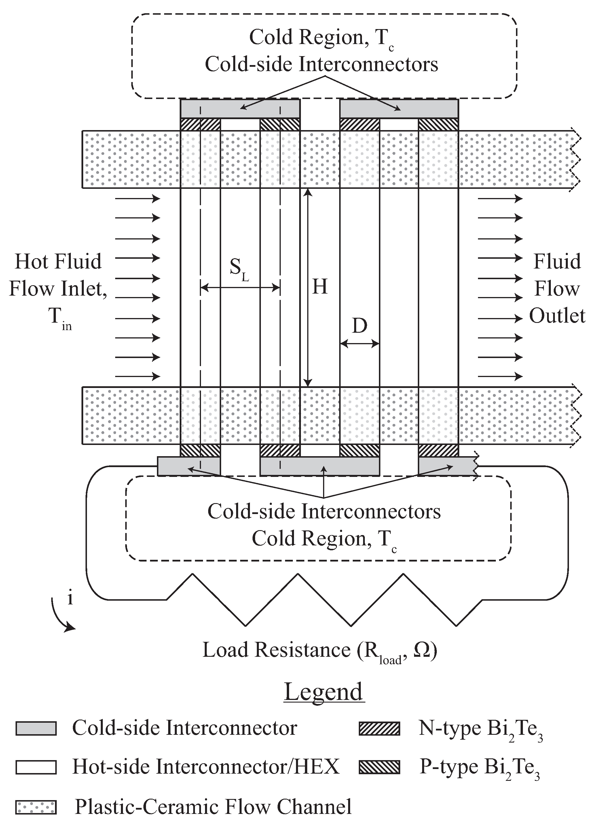
Figure 2.
Top-down view of an integrated thermoelectric device, showing the transverse and longitudinal spacing, and , respectively, of the pin-fin heat exchanger, the packing density , pin and pellet diameter D and flow channel width W.
Figure 2.
Top-down view of an integrated thermoelectric device, showing the transverse and longitudinal spacing, and , respectively, of the pin-fin heat exchanger, the packing density , pin and pellet diameter D and flow channel width W.
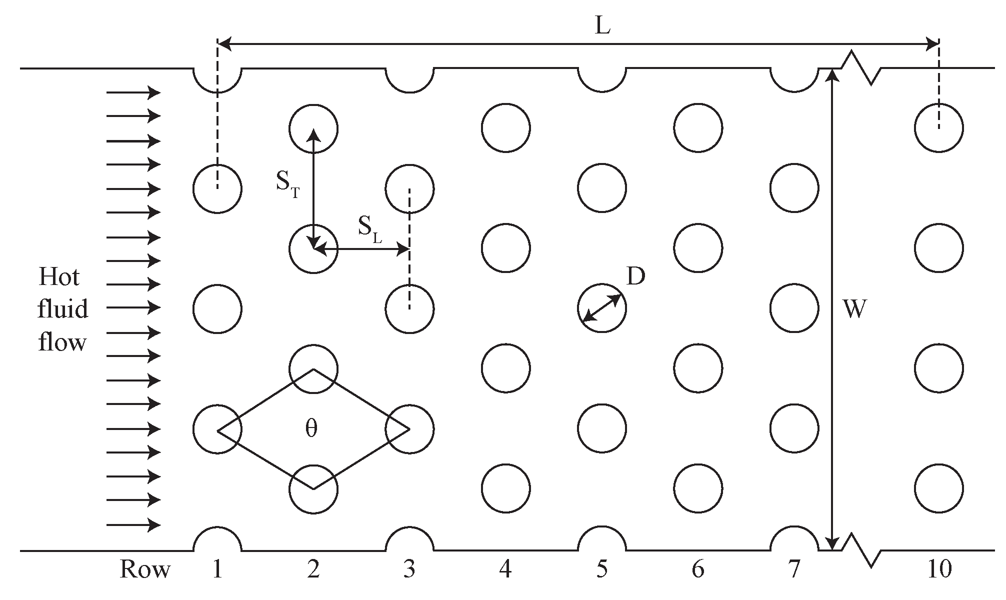
Figure 3.
Depiction of the solid domains within the iTED. Note, all top and bottom surfaces of upper and lower interconnectors are kept at a constant cold-side temperature of 300 K. The coarse mesh is overlaid on the last row of interconnectors, pellets, and rods.
Figure 3.
Depiction of the solid domains within the iTED. Note, all top and bottom surfaces of upper and lower interconnectors are kept at a constant cold-side temperature of 300 K. The coarse mesh is overlaid on the last row of interconnectors, pellets, and rods.
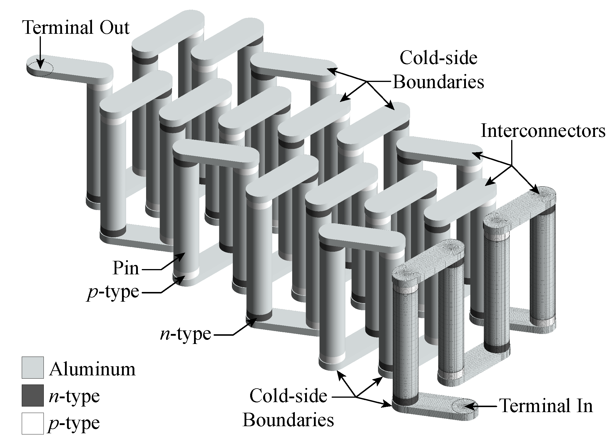
Figure 4.
Mesh of the fluid domain, with top-down views of the coarse (13,793,220 control volumes), medium (30,827,174 control volumes), and fine (69,190,554 control volumes) density grids.
Figure 4.
Mesh of the fluid domain, with top-down views of the coarse (13,793,220 control volumes), medium (30,827,174 control volumes), and fine (69,190,554 control volumes) density grids.
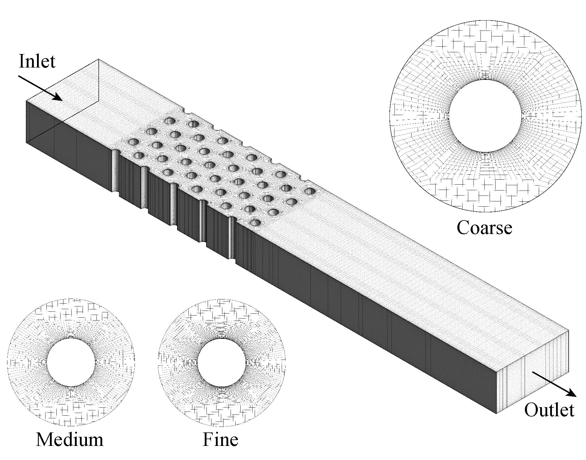
Figure 5.
Average hot-side junction temperature, for the a) integrated and b) conventional Bi2Te3 devices for all Re and conditions.
Figure 5.
Average hot-side junction temperature, for the a) integrated and b) conventional Bi2Te3 devices for all Re and conditions.
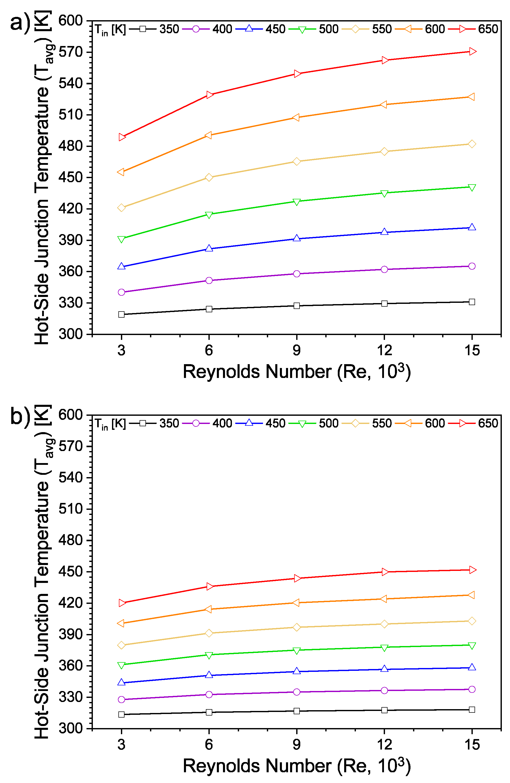
Figure 6.
Variation of internal electrical resistance with inlet flow rate, Re, and inlet fluid temperature, , for a) integrated and b) conventional thermoelectric devices.
Figure 6.
Variation of internal electrical resistance with inlet flow rate, Re, and inlet fluid temperature, , for a) integrated and b) conventional thermoelectric devices.
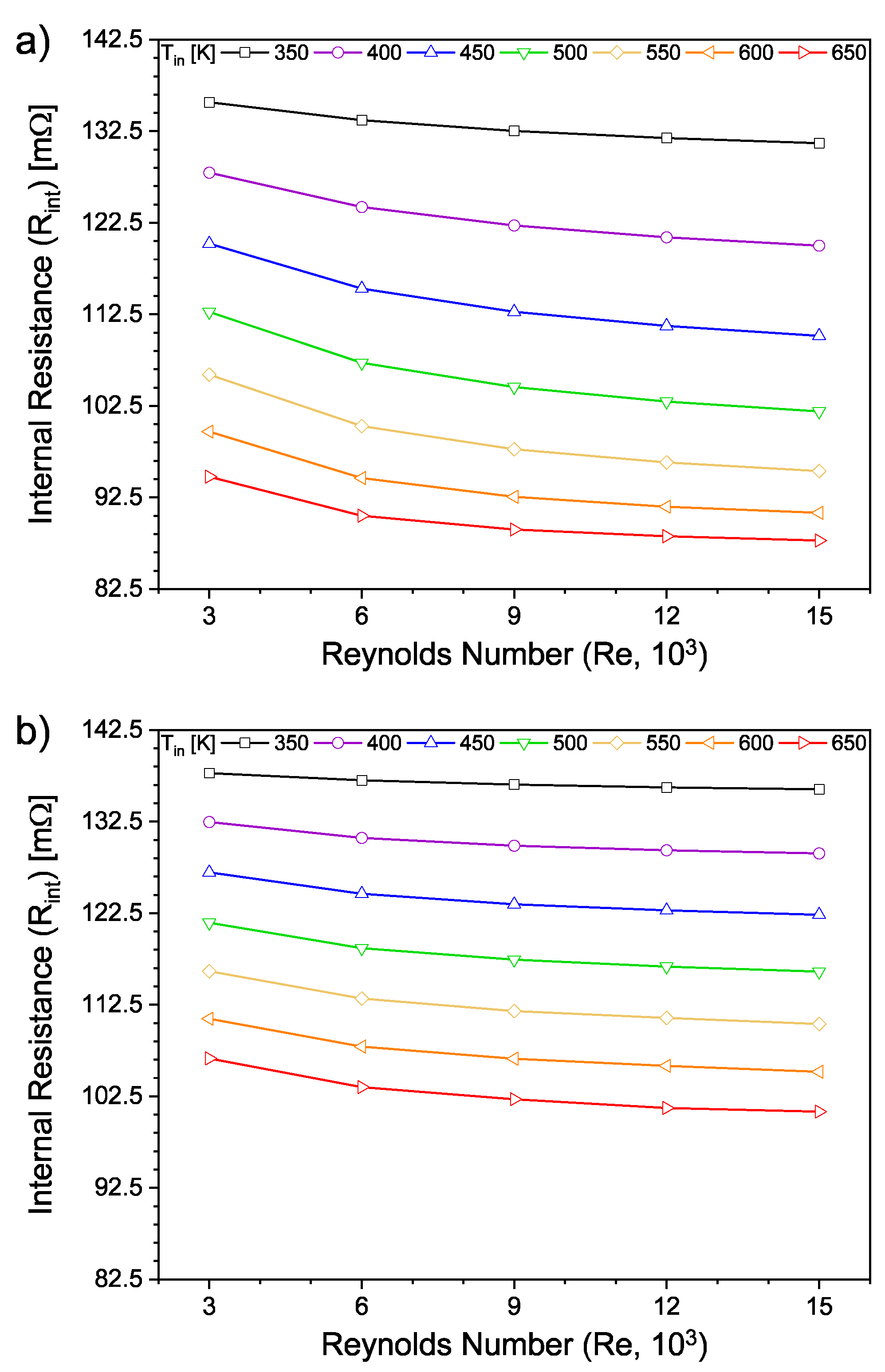
Figure 7.
Variation of with inlet flow rate, Re, and inlet fluid temperature, , for a) integrated and b) conventional thermoelectric devices.
Figure 7.
Variation of with inlet flow rate, Re, and inlet fluid temperature, , for a) integrated and b) conventional thermoelectric devices.
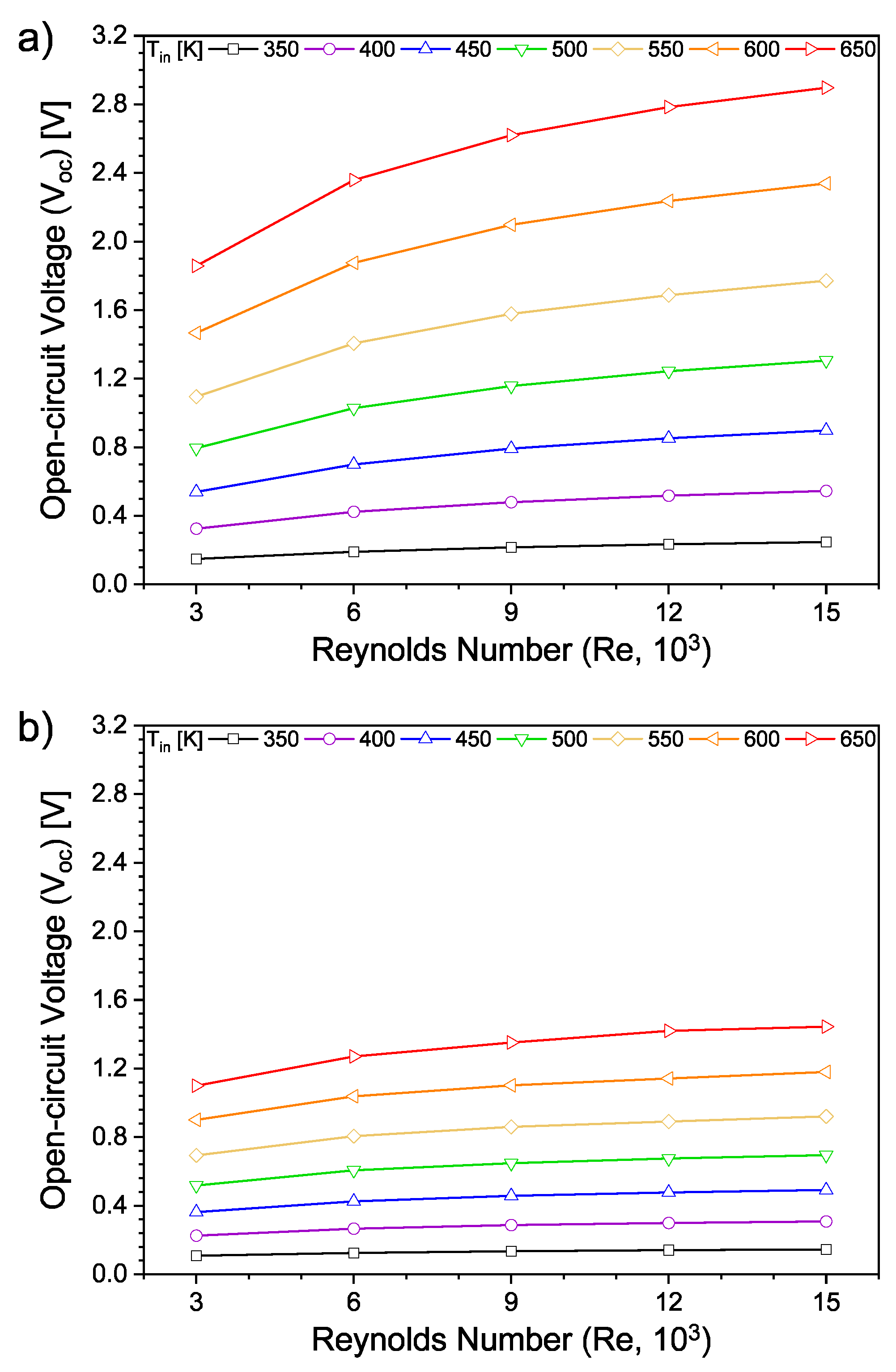
Figure 8.
Development of the Seebeck electromotive force (SEMF) within the device, with Re = 15,000, K.
Figure 8.
Development of the Seebeck electromotive force (SEMF) within the device, with Re = 15,000, K.
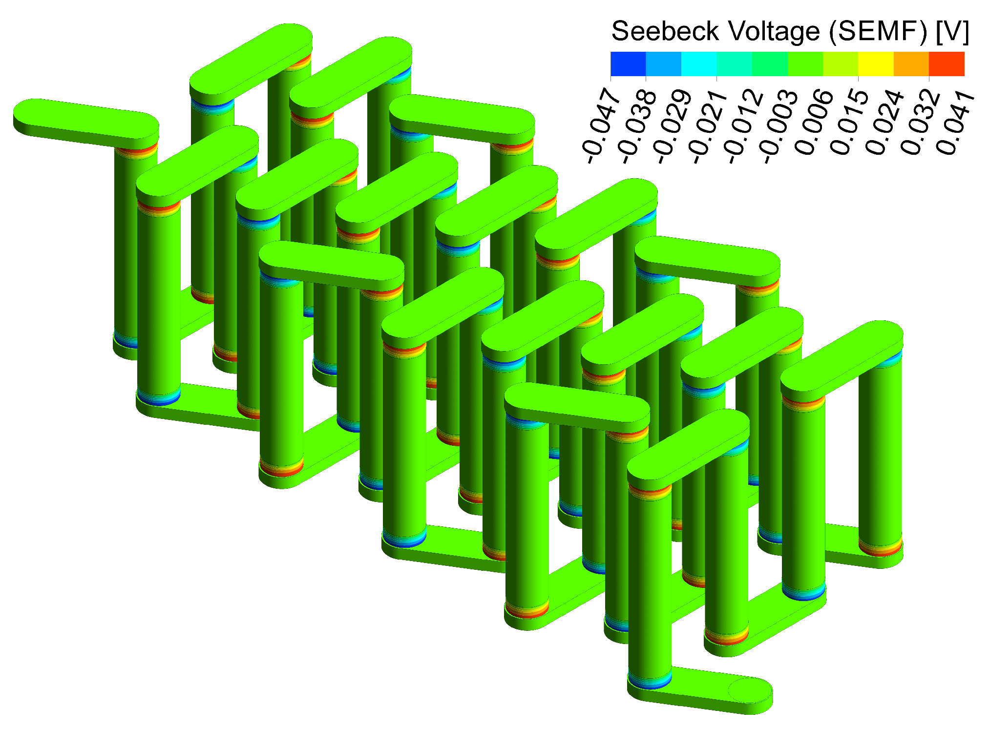
Figure 9.
Development of the electric potential (EP) across the device, with Re = 15,000, K.
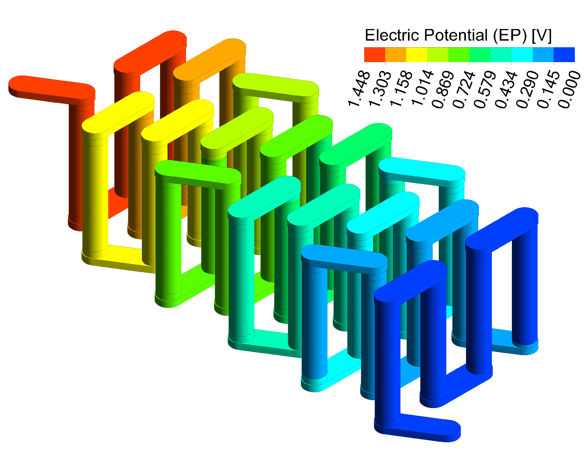
Figure 10.
Variation of I with inlet flow rate, Re, and inlet fluid temperature, , for a) integrated and b) conventional thermoelectric devices.
Figure 10.
Variation of I with inlet flow rate, Re, and inlet fluid temperature, , for a) integrated and b) conventional thermoelectric devices.
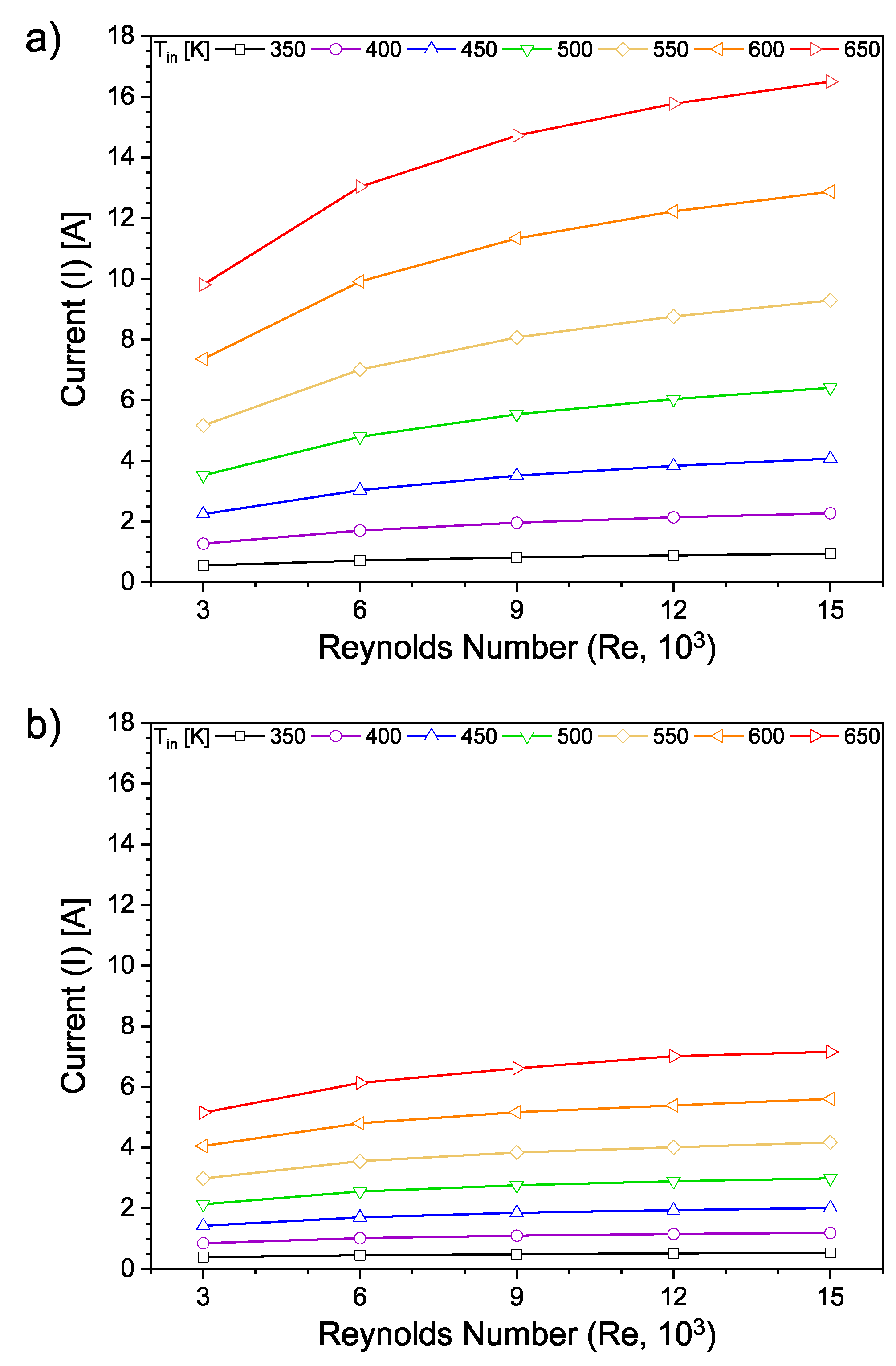
Figure 11.
Variation of with inlet flow rate, Re, and inlet fluid temperature, , for a) integrated and b) conventional thermoelectric devices.
Figure 11.
Variation of with inlet flow rate, Re, and inlet fluid temperature, , for a) integrated and b) conventional thermoelectric devices.
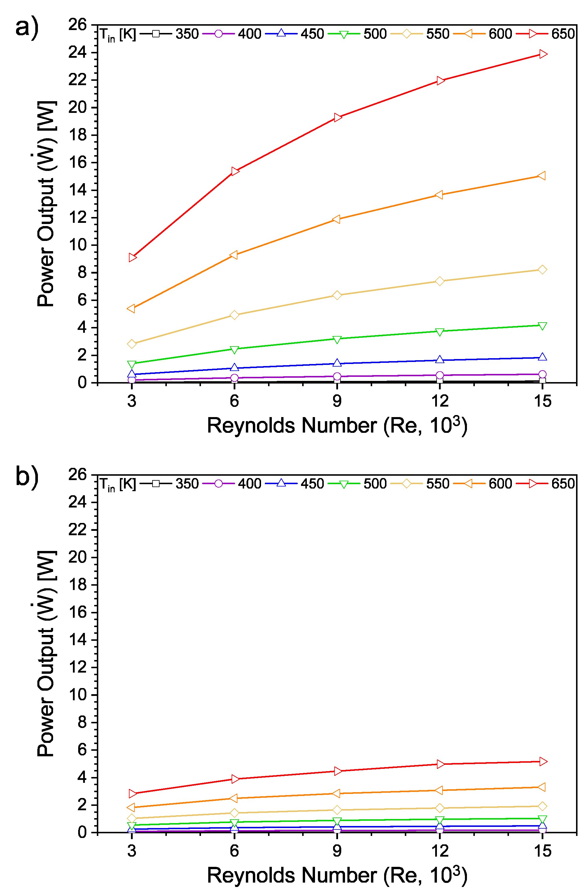
Figure 12.
Comparison of with inlet flow rate, Re, and inlet fluid temperature, , for a) integrated and b) conventional thermoelectric devices.
Figure 12.
Comparison of with inlet flow rate, Re, and inlet fluid temperature, , for a) integrated and b) conventional thermoelectric devices.
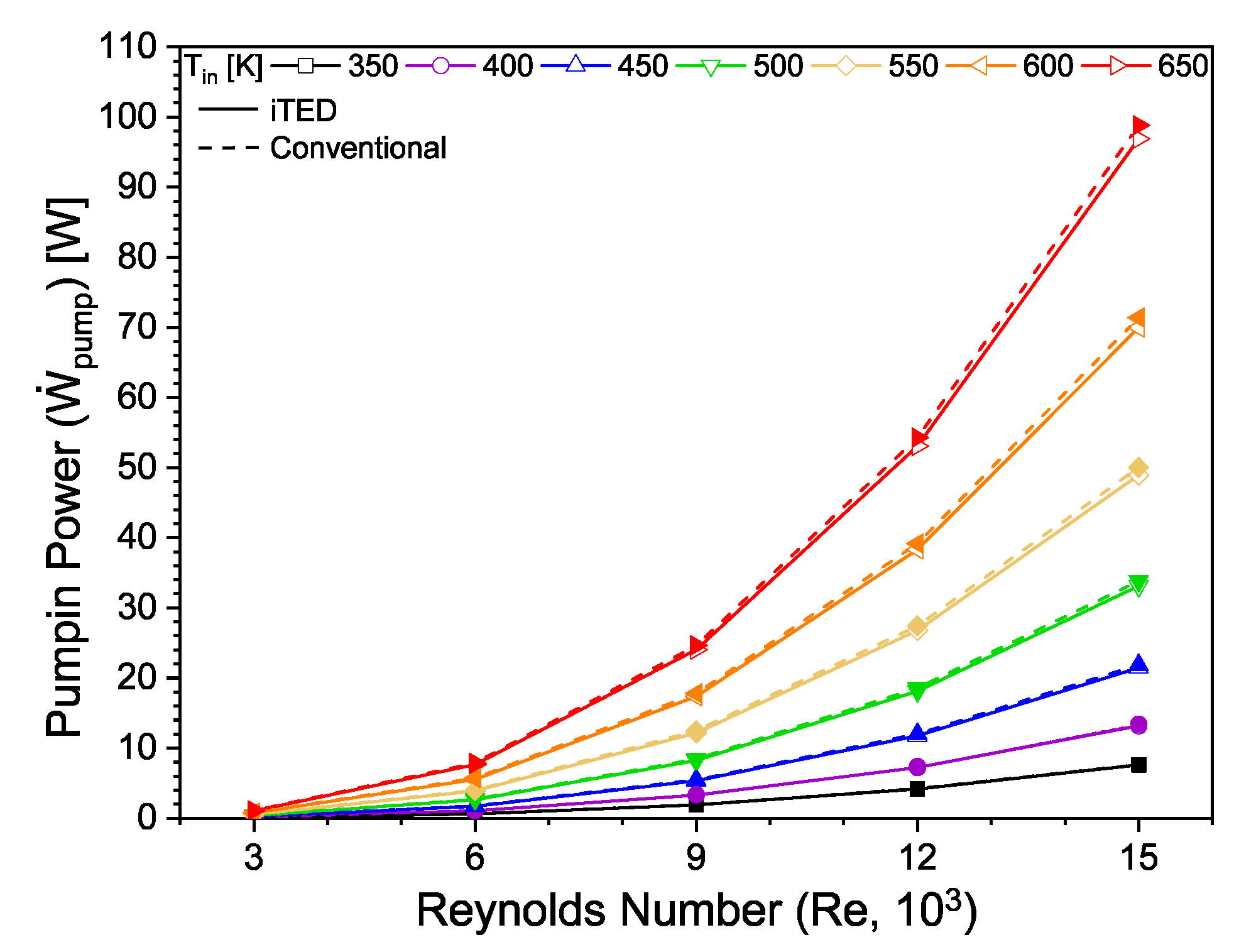
Figure 13.
Comparison of with inlet flow rate, Re, and inlet fluid temperature, , for a) integrated and b) conventional thermoelectric devices.
Figure 13.
Comparison of with inlet flow rate, Re, and inlet fluid temperature, , for a) integrated and b) conventional thermoelectric devices.
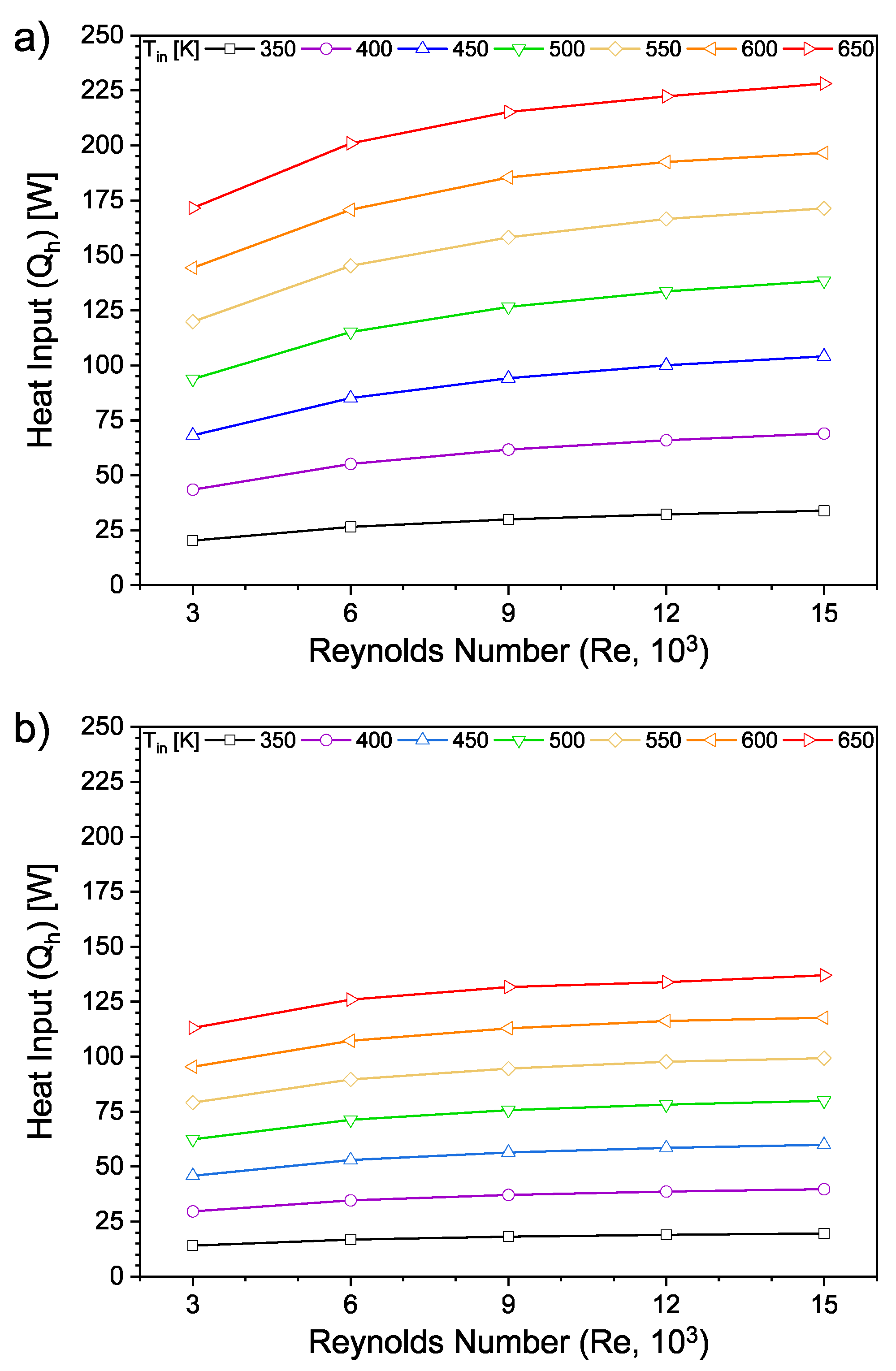
Figure 14.
Variation of with inlet flow rate, Re, and inlet fluid temperature, , for a) integrated and b) conventional thermoelectric devices.
Figure 14.
Variation of with inlet flow rate, Re, and inlet fluid temperature, , for a) integrated and b) conventional thermoelectric devices.
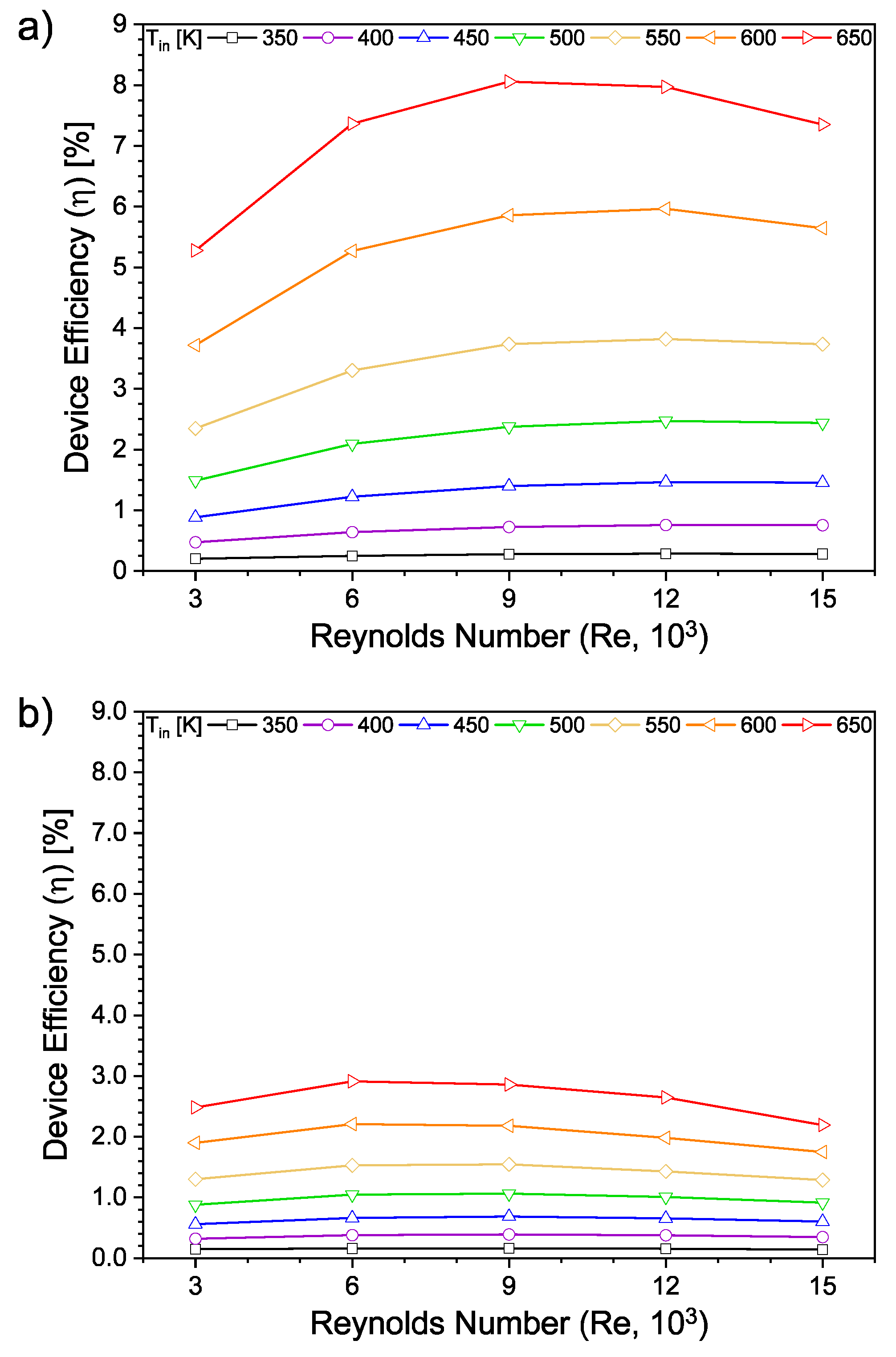
Figure 15.
Variation of with inlet flow rate, Re, and inlet fluid temperature, , for a) integrated and b) conventional thermoelectric devices.
Figure 15.
Variation of with inlet flow rate, Re, and inlet fluid temperature, , for a) integrated and b) conventional thermoelectric devices.
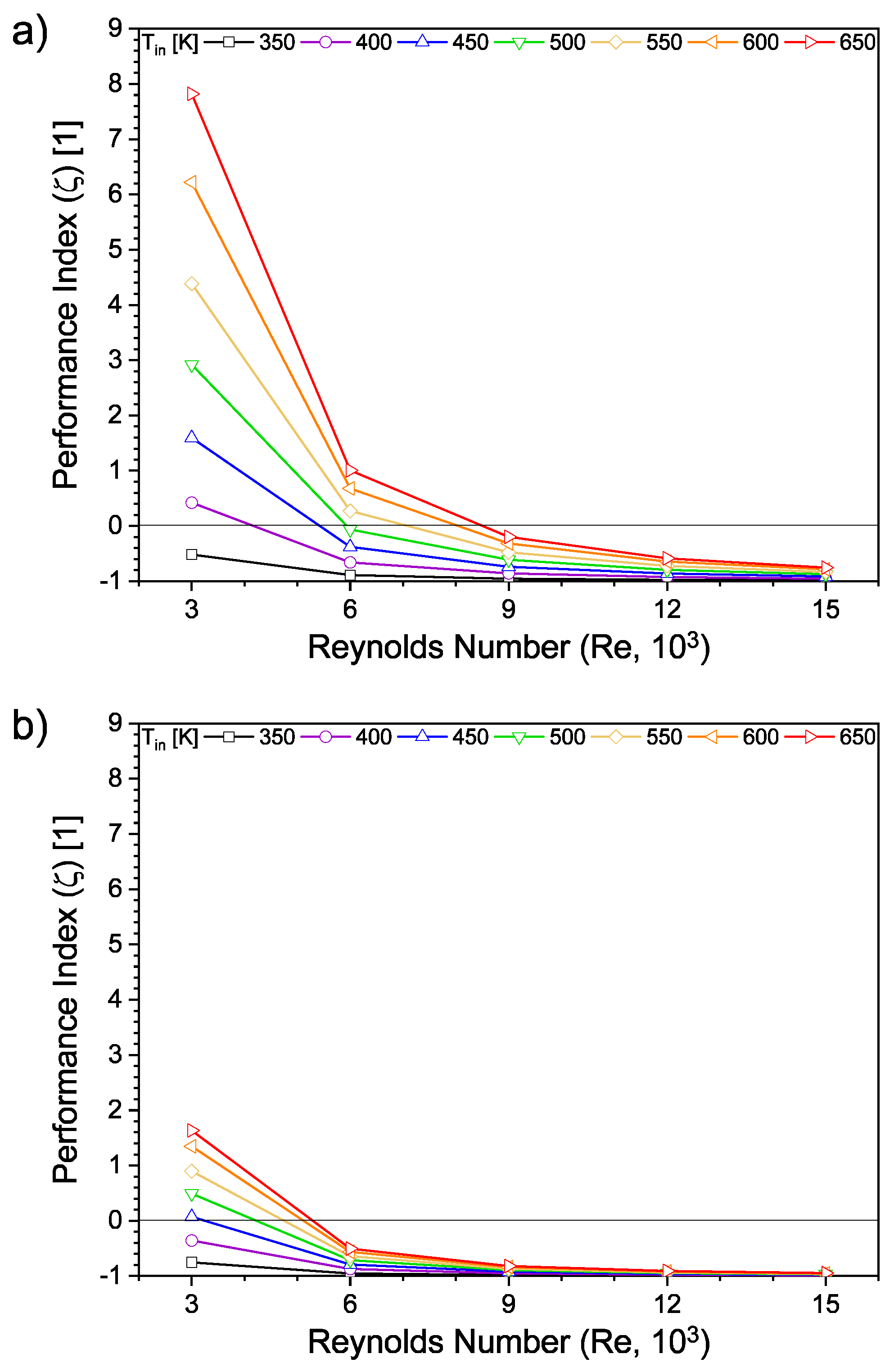
Figure 16.
Variation of I, , and with for Re=10,000 and K.
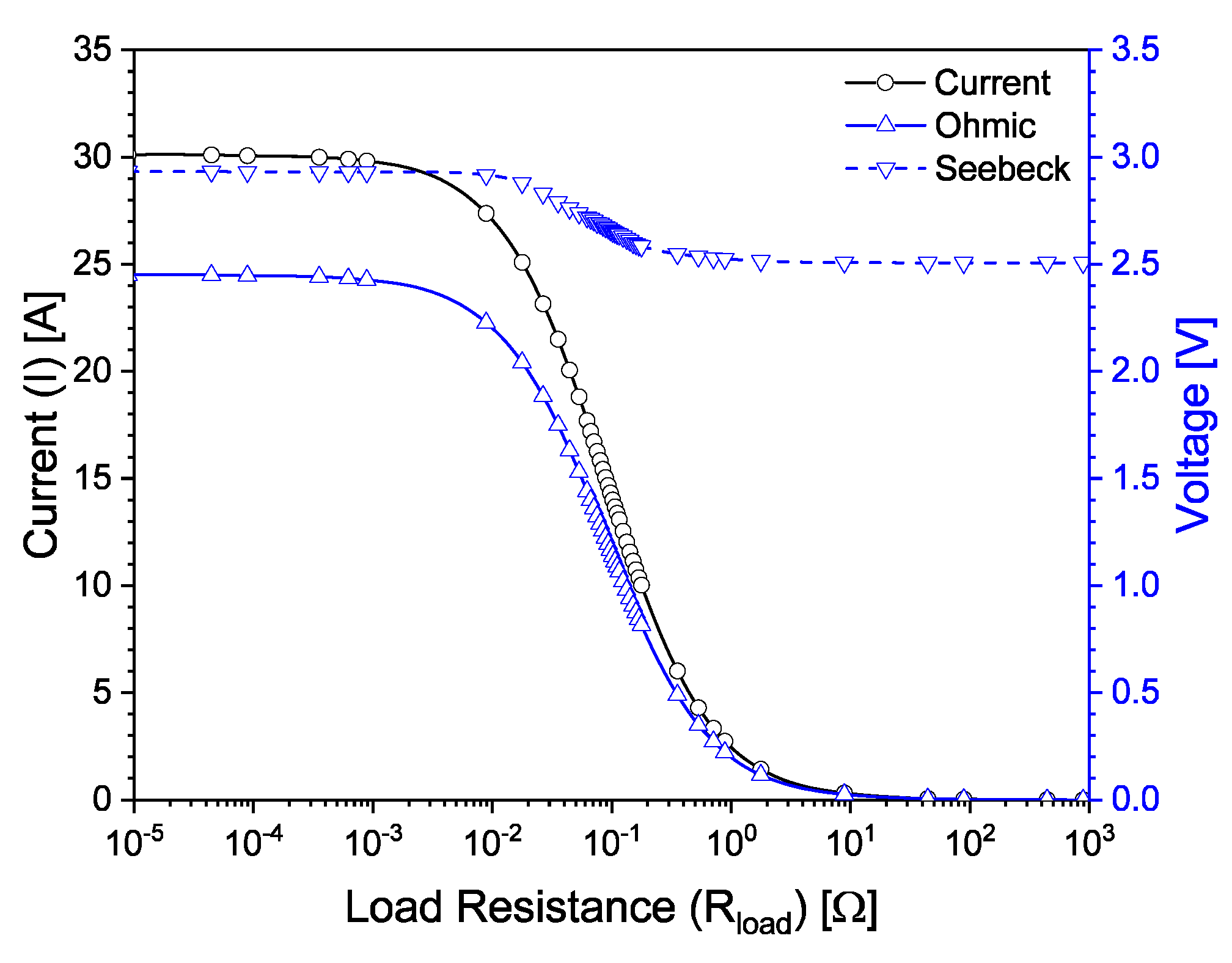
Figure 17.
Variation of and with for Re=10,000 and K.
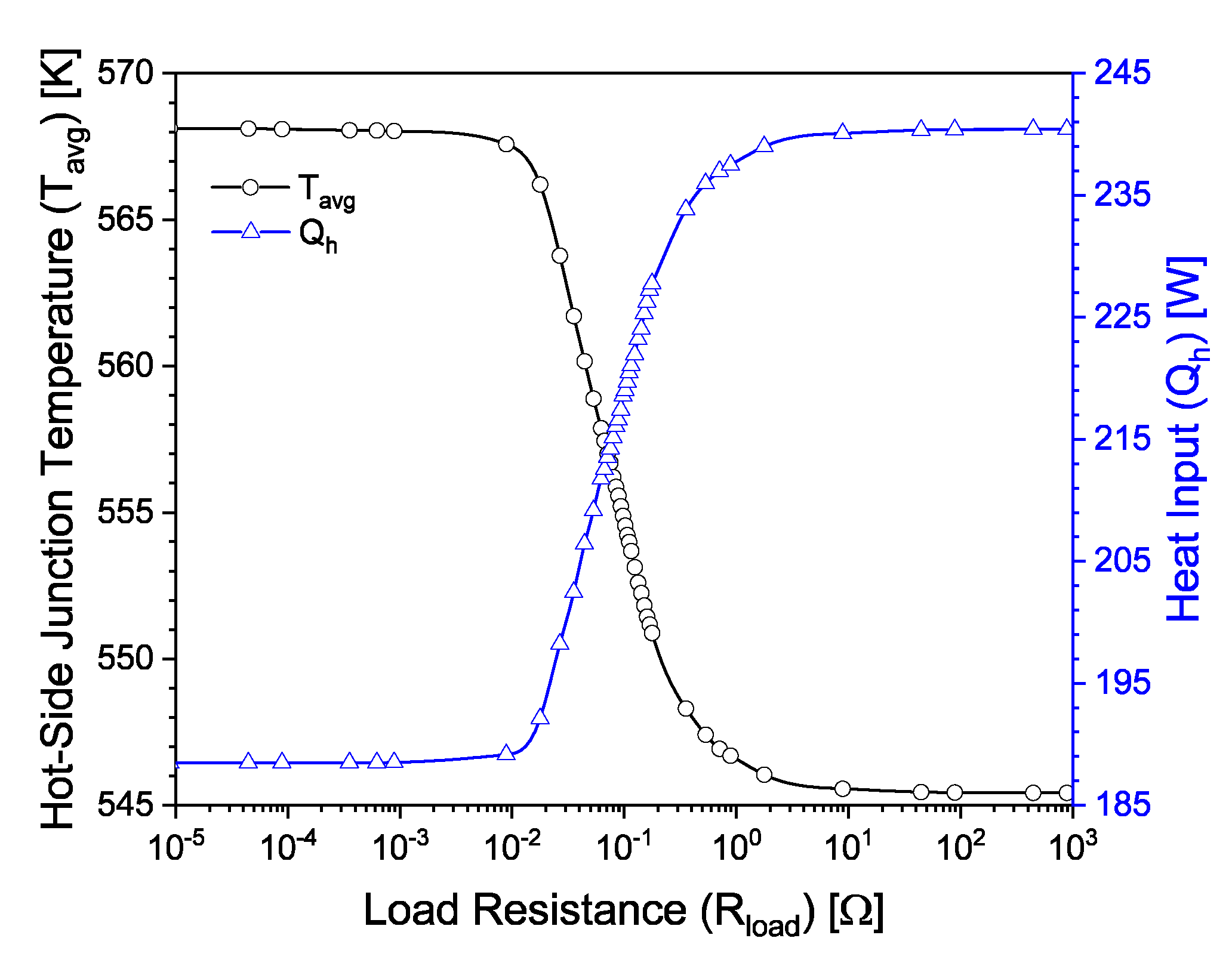
Figure 18.
Variation of and with for Re = 10,000 and K.
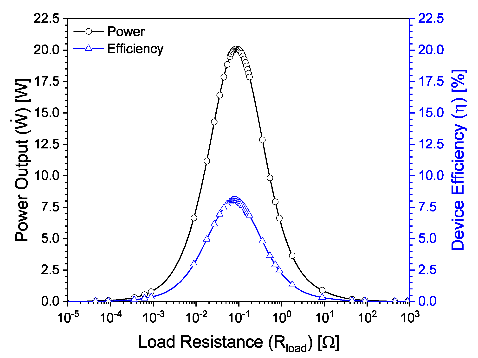
Figure 19.
Variation of with for Re = 10,000 and K.
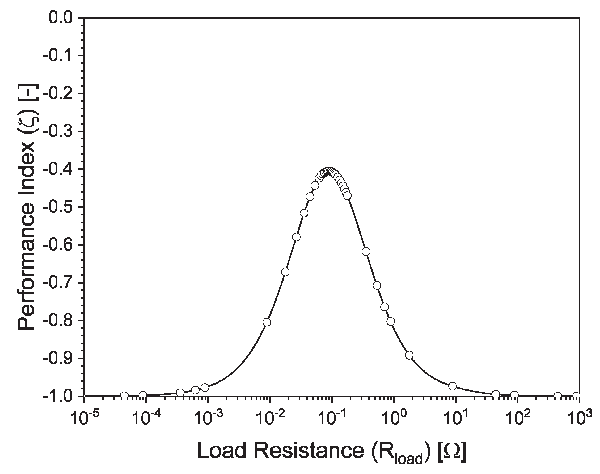

Table 1.
Polynomial expressions for temperature dependent thermoelectric properties for Bi2Te3 n[41]- and p-type[42], aluminum, alumina [39] and air [43] materials used in numerical calculations. All polynomial fits are valid from 300 to 650 K.
| Material | Property | Temperature Dependent Polynomial Expression |
|---|---|---|
| Bi2Te3 | = (1e-4)((2.1e-8) - (2.335e-5) + (6.517e-3)T -1.827) | |
| = (-3.054e-9) + (1.556e-5) - (0.01333)T + 4.275 | ||
| = (1e-5)((-2.387e-8) + (5.466e-5) - (3.691e-2)T + 8.531) | ||
| = (1e-5)((-9.167e-6) + (5.717e-2)T - 8.18) | ||
| = (-2.642e-3)T + 3.106 | ||
| = (1e-5)((-1.885e-8) + (4.341e-5) - (2.953e-2)T + 6.897) | ||
| Al | = (-8.454e-12) + (2.397E-8) - (2.468e-5) + (1.158e-2) - (2.475)T + 430.7 | |
| = (2.87132e-9) - (1.09328e-5) + (1.72806e-2) - (14.6213) + (7.08116e+3) - (1.92244e+6)T + 2.55322e+8 | ||
| Al2O3 | = (2.7092e-11) - (1.3607e-7) + (2.607E-4) - (0.22972)T + 85.868 | |
| Air | = (1.796e-11) - (4.231e-8) + (3.925e-5) - (0.0179)T + 4.01 | |
| = (-4.214e-7) + (9.151e-4) - (0.4125)T + 1064 | ||
| = (-9.724e-9) + (7.279e-5)T + 5.047e-3 | ||
| = (-1.917e-11) + (5.796e-8)T + 2.88e-6 |
Table 2.
Grid independence study for coarse (13,793,220 control volumes), medium (30,827,174 control volumes) and fine (69,190,554 control volumes) meshes for the inlet conditions of Re = 15,000 and = 650 K for both the integrated and conventional device configurations comprised of Bi2Te3. Reported absolute percent differences are between medium and coarse, and fine and medium meshes.
| Parameter | Coarse | Medium | |%| | Fine | |%| | |
| Conventional | [] | 0.101 105 00 | 0.100 896 20 | 0.103 | 0.100 829 77 | 0.03 |
| [V] | 1.312 933 | 1.432 867 | 4.368 | 1.443 598 | 0.37 | |
| I [A] | 6.492 919 | 7.100 701 | 4.471 | 7.158 593 | 0.41 | |
| [W] | 4.262 384 | 5.087 182 | 8.822 | 5.167 067 | 0.78 | |
| [W] | 99.312 | 99.007 | 0.154 | 98.839 | 0.08 | |
| [W] | 108.364 | 137.451 | 11.833 | 136.974 | 0.17 | |
| [%] | 2.052 | 2.151 | 2.356 | 2.191 | 0.92 | |
| [-] | -0.958 | -0.949 | 0.472 | -0.948 | 0.05 | |
| Integrated | [] | 0.087 263 | 0.087 843 | 0.663 | 0.087 793 | 0.057 |
| [V] | 2.651 158 | 2.892 519 | 8.708 | 2.896 883 | 0.151 | |
| I [A] | 15.190 560 | 16.464 046 | 8.046 | 16.498 210 | 0.207 | |
| [W] | 20.136 289 | 23.811 284 | 16.724 | 23.896 698 | 0.358 | |
| [W] | 97.107 | 97.063 | 0.045 | 96.901 | 0.167 | |
| [W] | 239.514 | 229.263 | 4.374 | 228.117 | 0.501 | |
| [%] | 5.982 | 7.297 | 19.806 | 7.352 | 0.751 | |
| [-] | -0.793 | -0.755 | 4.910 | -0.753 | 0.265 |
Disclaimer/Publisher’s Note: The statements, opinions and data contained in all publications are solely those of the individual author(s) and contributor(s) and not of MDPI and/or the editor(s). MDPI and/or the editor(s) disclaim responsibility for any injury to people or property resulting from any ideas, methods, instructions or products referred to in the content. |
© 2026 by the authors. Licensee MDPI, Basel, Switzerland. This article is an open access article distributed under the terms and conditions of the Creative Commons Attribution (CC BY) license.
Copyright: This open access article is published under a Creative Commons CC BY 4.0 license, which permit the free download, distribution, and reuse, provided that the author and preprint are cited in any reuse.


