
Submitted:
21 January 2026
Posted:
21 January 2026
You are already at the latest version
Abstract
Background: Prognostic prediction for colorectal cancer patients with peritoneal metastasis remains challenging due to clinical and biological heterogeneity. We aimed to evaluate the utility of machine learning, comparing high-performance boosting models with interpretable regression approaches for overall survival (OS) prediction. Methods: We analyzed a multi-institutional registry cohort of 150 colorectal cancer patients with synchronous peritoneal metastases. A total of 124 variables were included; continuous variables were standardized, categorical variables were one-hot encoded, and missing values were imputed using the median. Models included XGBoost, LightGBM, Ridge regression, Lasso regression, and linear regression. Training was performed with 3-fold cross-validation, and hyperparameters were optimized using Optuna. Evaluation metrics included mean absolute error (MAE), root mean square error (RMSE), and coefficient of determination (R²). Model interpretability was assessed using SHAP values, LIME local explanations, and regression coefficients. Results: Boosting models consistently outperformed linear models. XGBoost achieved the best performance (MAE 424, RMSE 526, R² = 0.04), while LightGBM showed comparable accuracy. In contrast, Ridge, Lasso, and Linear regression yielded high errors (MAE > 900, RMSE > 1200) with negative R² values, indicating poor predictive ability. SHAP analysis highlighted systemic inflammation markers (CRP, BUN), surgical assessment of tumor depth, operative factors (time, bleeding), and peritoneal metastasis characteristics as major determinants of OS. LIME analyses further provided case-specific interpretability, identifying feature contributions in long-, intermediate-, and short-term survivors. Conclusion: Boosting models, particularly XGBoost, demonstrated superior performance compared with traditional regression models in predicting OS for colorectal cancer patients with peritoneal metastasis, although absolute predictive accuracy remains modest. Integration of SHAP and LIME linked model outputs with clinically plausible prognostic factors, enhancing interpretability. Ensemble learning may provide a promising adjunct for prognostic assessment and should be validated in larger, genomically enriched cohorts.
Keywords:
colorectal cancer
; peritoneal metastasis
; cytoreductive surgery
; hyperthermic intraperitoneal chemotherapy
; machine learning
; XGBoost
; LightGBM
; SHAP
; LIME
; prognosis
1. Introduction
Colorectal cancer (CRC) is the third most common malignancy worldwide and a leading cause of cancer-related mortality. Peritoneal metastasis of colorectal cancer (CRC-PM) represents one of the most challenging clinical scenarios, with dismal prognosis despite advances in systemic chemotherapy, cytoreductive surgery (CRS), and hyperthermic intraperitoneal chemotherapy (HIPEC). [1,2,3,4,5] Prognostic prediction of overall survival (OS) is essential for tailoring treatment strategies, guiding adjuvant therapy, and counseling patients. Conventional prognostic approaches, including TNM staging and clinicopathological scoring systems [1,4], provide valuable population-level insights but lack precision for individualized risk estimation [6,7,8]. This project is currently establishing a new classification for peritoneal metastasis in Japan [9].
In recent years, machine learning (ML) has emerged as a promising tool for clinical prediction tasks [10,11,12,13,14,15] . Boosting algorithms such as XGBoost (eXtreme Gradient Boosting) and LightGBM(Light Gradient Boosting Machine) have achieved state-of-the-art performance across domains [16], yet their limited interpretability raises barriers to clinical adoption. Conversely, linear models (Ridge, Lasso, Linear regression) offer transparency but often sacrifice predictive accuracy.
To date, limited studies have directly compared high-performance and interpretable ML approaches in the context of CRC OS prediction. This study therefore aimed to (1) assess the feasibility of ML-based OS prediction, and (2) compare boosting-based and linear models to highlight the trade-off between accuracy and interpretability in clinical prognostication.
2. Materials and Methods
2.1. Study design
The 28 member hospitals of the Japanese Society for Cancer of the Colon and Rectum (JSCCR) participated in this multi-institutional observational study conducted by the JSCCR committee “Grading of Peritoneal Metastasis from Colorectal Cancer.” One hundred fifty patients who underwent surgery for colorectal cancer with synchronous peritoneal metastases between October 2012 and December 2016 were enrolled, and clinical/pathological data were registered within 3 months after surgery. Prognostic information was collected 3 years after surgery. Written, informed consent was obtained from all patients before enrollment. Since synchronous peritoneal metastases from colorectal cancer are often found accidentally during surgery, written informed consent could be obtained after surgery in such cases. The ethics committees of the JSCCR and each institution approved this study. In this study, tumor location was classified into right colon (appendix, cecum, ascending colon, transverse colon), left colon (descending colon, sigmoid colon), and rectum (Rectosigmoid; RS, upper rectum; Ra, lower rectum; Rb).
2.2. Surgical procedure
The surgical procedure was not determined by the protocol of this study, because there are a variety of conditions in patients with synchronous peritoneal metastases. Each surgeon made a decision about primary tumor resection and peritoneal metastasis resection.
2.3. Variables
A total of 124 clinical, pathological, and laboratory variables were considered as candidate predictors in Table 1.
2.4. Model Training and Evaluation
We compared high-performance machine learning models (XGBoost and LightGBM) with interpretable models (Ridge regression, Lasso regression, and Linear regression). For preprocessing, continuous variables were standardized, while categorical variables were converted using one-hot encoding. Missing values were handled by median imputation.
Model training was conducted using 3-fold cross-validation, and hyperparameter optimization was performed with the Optuna framework. Model performance was evaluated using both graphical and quantitative approaches. Graphical assessments included predicted versus observed overall survival (OS) scatter plots, residual plots, and error distribution histograms. Model interpretability was examined with SHAP summary and dot plots as well as LIME local explanations for boosting models, and regression coefficients for linear models.
Quantitative evaluation included mean absolute error (MAE), root mean square error (RMSE), and coefficient of determination (R²) as primary performance metrics. These complementary evaluations allowed us to compare both predictive accuracy and model interpretability across different algorithms.
3. Results
3.1. Patient Characteristics
A total of 150 patients were included in the analysis. Baseline characteristics are summarized in Table 2. The median age was 66 years [range, 30–89], and 56.0% of patients were male. The median BMI was 20.8 [range, 9.4–40.5] kg/m². Comorbidities were observed in most frequently hypertension (26.0%) and diabetes mellitus (14.0%). The primary tumor was located in the right colon in 53%, in the left colon in 29% and in the rectum in 18%. Median laboratory values included WBC 6800/μL, hemoglobin 11.6 g/dL, platelet count 30.5 ×10⁴/μL, albumin 3.6 g/dL, CRP 0.7 mg/dL, CEA 23.3 ng/mL, and CA19-9 48.5 U/mL. The median operative time was 191.5 minutes, and median blood loss was 123.5 mL. The median overall survival was 635 days [range, 21–2358]. According to the present Japanese classification, the number of patients with synchronous peritoneal metastases was 30 (20%) in P1, 57 (38%) in P2, and 63 (42%) in P3. The median PCI was 4 (range, 1–29). The median follow-up days of the surviving patients and median follow-up days of the dead patients were 1364 days [range, 21–2340] and 535 days [range, 33–2358].
3.2. Predictive Performance
In this study, we compared high-performance machine learning models (XGBoost, LightGBM) with interpretable linear models (Ridge, Lasso, Linear regression) for predicting overall survival. Boosting models consistently outperformed linear models. XGBoost achieved the lowest prediction error (MAE 424, RMSE 526) with a modest explanatory ability (R² = 0.04), while LightGBM showed similar performance but nearly zero R². In contrast, linear approaches performed poorly, with high errors (MAE > 900, RMSE > 1200) and strongly negative R² values, indicating a lack of predictive capability and potential overfitting (Table 3).
These findings highlight that boosting methods, particularly XGBoost, can capture complex, non-linear patterns in survival data, whereas linear models fail to adequately reflect the prognostic heterogeneity of colorectal cancer with peritoneal metastasis. Although the absolute predictive accuracy remains modest, the results suggest that ensemble learning offers a more promising framework for survival prediction compared to traditional regression-based approaches.
Figure 1.
Predicted versus observed overall survival across five models. Scatter plots demonstrate the relationship between predicted and observed OS for XGBoost (A), LightGBM (B), Ridge regression (C), Lasso regression (D), and Linear regression (E). The diagonal line indicates perfect prediction (y = x). Boosting models (A, B) showed closer alignment with the reference line, whereas linear models (C–E) exhibited large deviations and wider scatter, reflecting inferior predictive performance.
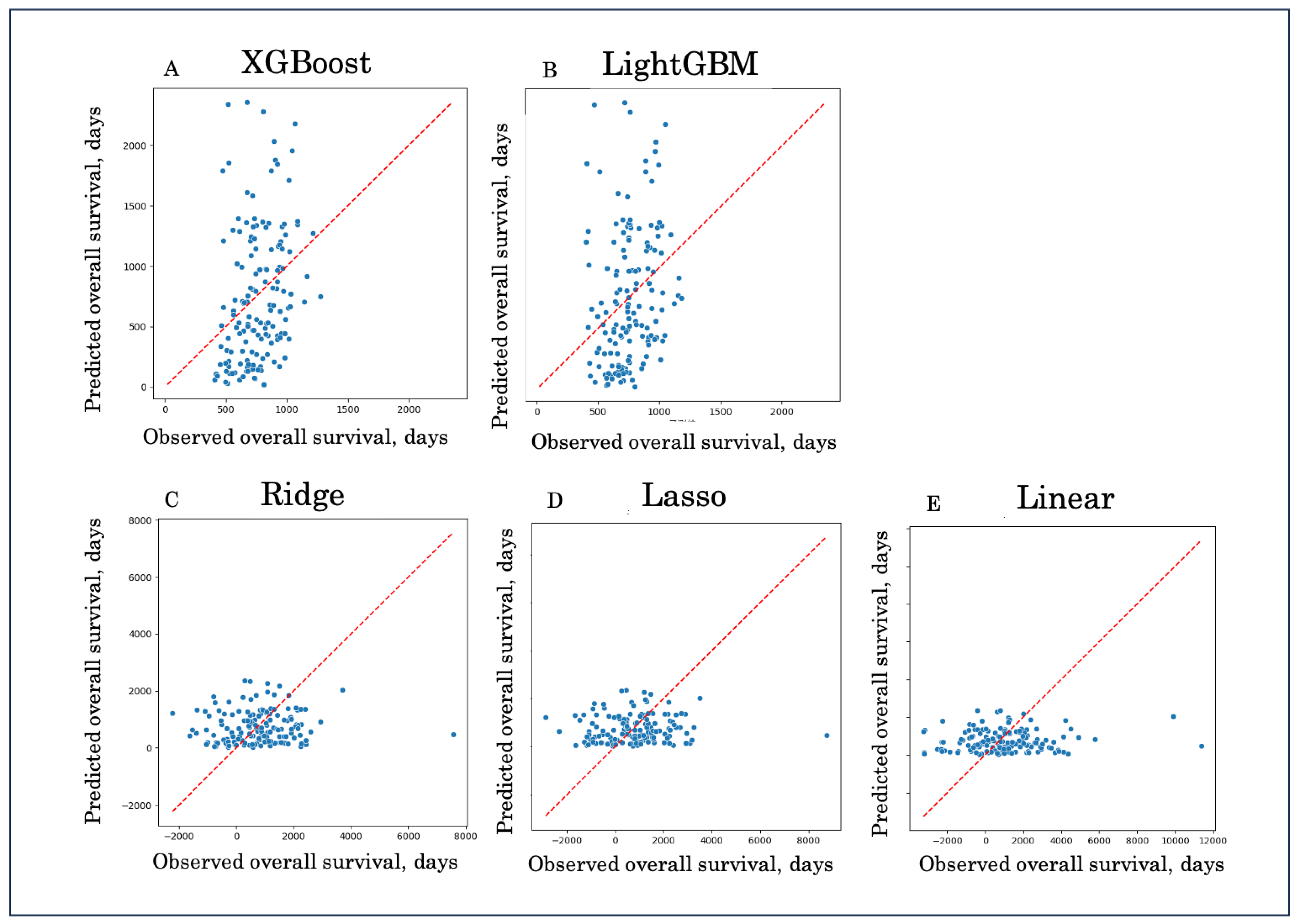
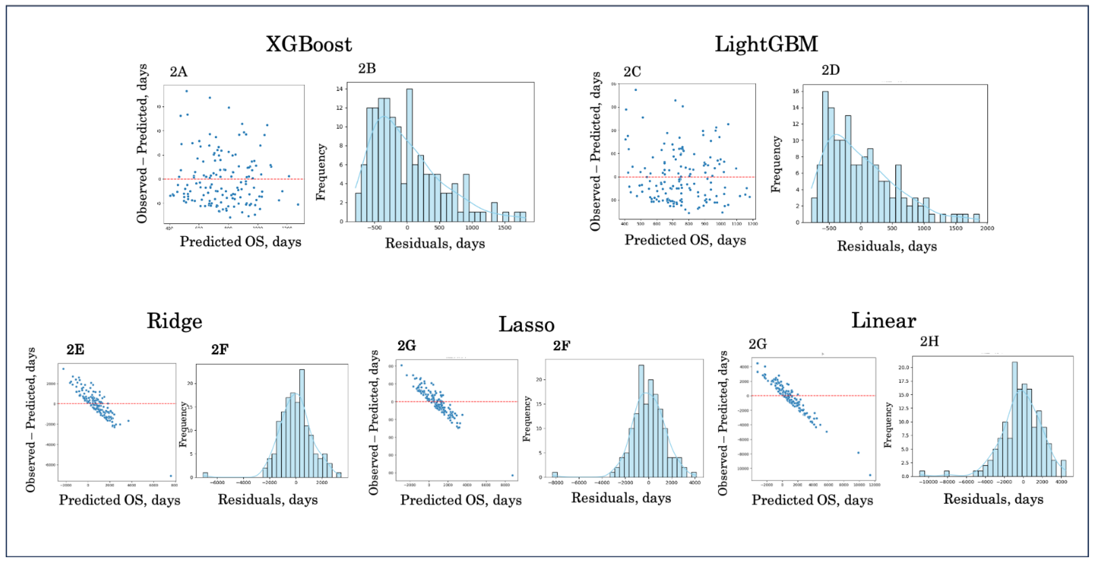
Figure 2.
Residual and error distribution plots. Residual plots (left panels) and error distribution histograms (right panels) are shown for XGBoost (A, B), LightGBM (C, D), Ridge regression (E, F), Lasso regression (G, H), and Linear regression (I, J). Boosting models (A–D) demonstrated residuals centered closer to zero and narrower error distributions, indicating better calibration and reduced bias. In contrast, linear models (E–J) exhibited wider and asymmetric error distributions, reflecting poorer predictive accuracy and systematic deviation from observed survival.
3.3. Interpretability
Global feature importance derived from SHAP analysis is shown in Figure 3. Both XGBoost and LightGBM identified systemic inflammation markers (CRP, BUN), surgical assessment of tumor depth, and peritoneal metastasis–related variables (e.g., residual PCI regions, dissemination diameter) as key determinants of overall survival, with operative time and CA19-9 further contributing to prediction.
To illustrate model interpretability at the individual level, we performed LIME local explanations on representative survival cases using XGBoost with and without Optuna tuning (Figure 4).
Case 1 (survival time: 491 days): Both models identified elevated CRP, high BUN, and prolonged operative time as major negative contributors, while tumor location in the sigmoid colon and lower TP supported survival. Optuna-tuned XGBoost additionally highlighted residual peritoneal disease (PCI region 8) and intraoperative blood loss as unfavorable predictors.
Case 2 (survival time: 506 days): In this intermediate survival case, favorable contributions included lower CRP and absence of heart disease, while unfavorable factors comprised high BUN, surgical depth of invasion, and residual dissemination. Optuna-tuned analysis emphasized weight, operative time, and PCI burden as critical drivers.
Case 3 (survival time: 2340 days): This long-term survivor exhibited positive contributions from low CRP, absence of residual dissemination, and favorable operative/pathological factors. Negative contributions included advanced tumor depth, high BUN, and extensive pelvic procedures. The Optuna-tuned model consistently confirmed residual disease in PCI regions and dissemination grade as key survival determinants.
These examples demonstrate how local interpretability methods can contextualize individual survival predictions by balancing favorable and unfavorable clinical and surgical features, thereby enhancing clinical plausibility of machine learning outputs.
4. Discussion
In this multi-institutional study, we developed and compared machine learning models to predict overall survival in patients with colorectal cancer and peritoneal metastasis. Our findings highlight that boosting-based ensemble models, particularly XGBoost [14], demonstrated superior predictive accuracy compared to traditional regression models, although the absolute predictive power remained modest. Linear approaches, including Ridge, Lasso, and standard regression [12,13], showed markedly inferior performance with high error rates and negative R² values, underscoring their limitations in modeling heterogeneous survival outcomes.
The improved performance of boosting models likely reflects their ability to capture complex, non-linear relationships between clinical, pathological, and perioperative variables and survival outcomes. SHAP analysis [12] further confirmed that key prognostic factors identified by the models—such as peritoneal dissemination grade [7,8], CA19-9, operative time, and nodal status—are consistent with established clinical knowledge. Recent studies have further demonstrated that SHAP enables both global and local interpretation of tree-based ensemble models, facilitating their application in clinical decision support systems [15] . LIME analyses [13] provided case-level interpretability, demonstrating how individual predictions were influenced by specific patient factors. These complementary approaches bridge the gap between machine learning predictions and clinical interpretability, a critical requirement for translational application in oncology [10,11] .
Despite these advantages, the overall R² values remained low, reflecting the intrinsic difficulty of survival prediction in this high-risk population. Peritoneal metastasis in colorectal cancer is influenced by multiple biological, surgical, and treatment-related factors [2,3,4,5] that may not be fully captured in routinely available clinical datasets. Previous studies have reported similar challenges, where machine learning approaches achieved incremental but not dramatic improvements over conventional indices. Our results are therefore consistent with the broader literature and highlight both the potential and the current limitations of machine learning in survival prediction [10,11] .
Although the coefficient of determination (R²) remained modest in the present study, this finding should be interpreted in the context of the clinical characteristics of colorectal cancer with peritoneal metastasis. Overall survival in this population is driven by highly heterogeneous and multifactorial processes, including tumor biology, extent and distribution of peritoneal disease, surgical decision-making, postoperative complications, and subsequent systemic treatments, many of which are not fully captured in registry-based clinical datasets. In such settings, low R² values have been consistently reported even in large-scale survival modeling studies and do not necessarily indicate a lack of clinical relevance. Instead, the observed improvement in absolute prediction error and consistent outperformance of boosting-based models over linear approaches suggest that ensemble learning captures meaningful non-linear patterns in survival outcomes. Importantly, the integration of interpretability methods such as SHAP and LIME demonstrated that model predictions were driven by clinically plausible prognostic factors, supporting the potential utility of these models for relative risk stratification rather than precise individual survival time estimation.
In line with these observations, an increasing body of literature has demonstrated the advantage of boosting-based ensemble models for survival prediction in oncology. Comparative studies using large registry-based datasets have shown that gradient boosting approaches, including XGBoost [14] and LightGBM [17], consistently outperform conventional Cox proportional hazards models and linear regression–based methods in terms of discrimination and overall predictive performance [18,19] . These findings suggest that the ability of boosting algorithms to model non-linear effects and complex interactions among heterogeneous clinical variables is particularly advantageous in advanced cancer populations, where prognosis is driven by multifactorial and interdependent processes [20,21] . Importantly, although the performance gains reported in these studies are generally modest, their consistent reproducibility across different cancer types and datasets supports the robustness and generalizability of boosting-based survival models [20,21] .
Clinically, these findings suggest that boosting models could be applied as adjunctive tools for risk stratification, particularly when combined with interpretability methods that align predictions with known prognostic markers. For instance, SHAP analysis emphasized peritoneal dissemination grade and CA19-9—both widely accepted prognostic factors [7,8] —thereby increasing clinician confidence in model outputs. However, until predictive accuracy improves further, such models should complement rather than replace traditional prognostic assessments [6] .
Several limitations must be acknowledged. First, although this was a multi-institutional study, the cohort size was relatively limited, and external validation was not performed. Second, the dataset contained missing values that were imputed, which may introduce bias. Third, molecular and genomic variables were not included, which could enhance predictive power if integrated in future studies. Finally, the modest R² values indicate that larger, richer datasets and integration of biological markers are needed to achieve clinically actionable prediction models.
Taken together, our findings indicate that ensemble learning methods such as XGBoost [14] and LightGBM [17] outperform linear regression models in this clinical setting. While predictive accuracy remains limited, the combination of boosting algorithms with interpretability tools such as SHAP [12] and LIME [13] provides a promising framework for future prognostic modeling. Further research with larger, genomically enriched datasets and external validation is warranted to refine these models and advance their clinical utility.
5. Conclusions
In conclusion, boosting-based ensemble learning models, particularly XGBoost and LightGBM, demonstrated superior predictive performance compared with linear regression models in forecasting overall survival among patients with colorectal cancer and peritoneal metastasis. While the absolute predictive accuracy remained limited, the integration of interpretability tools such as SHAP and LIME provided clinically meaningful insights by linking model predictions with established prognostic factors. These findings suggest that ensemble machine learning models may serve as promising adjuncts for prognostic assessment. Future studies incorporating larger cohorts, genomic markers, and external validation are warranted to further refine predictive accuracy and facilitate clinical translation.
Author Contributions
Conceptualization, Y.B.; methodology, Y.B.; software, Y.B.; validation, Y.B.; formal analysis, Y.B.; investigation, Y.B.; data curation, Y.B. with contributions from participating institutions of the JSCCR; resources, participating hospitals of the JSCCR; writing—original draft preparation, Y.B.; writing—review and editing, Y.B. in consultation with the institutional representatives who approved the manuscript contents; visualization, Y.B.; supervision, Y.B. All authors involved in data provision reviewed and agreed to the final version of the manuscript.
Funding
This research received no external funding.
Institutional Review Board Statement
The study was conducted in accordance with the Declaration of Helsinki, and approved by the Institutional Review Board of the Japanese Society for Cancer of the Colon and Rectum (JSCCR) and the ethics committees of all participating institutions.
Informed Consent Statement
A written informed consent was obtained from each patient.
Data Availability Statement
The data presented in this study are not publicly available due to institutional and ethical restrictions but are available from the corresponding author on reasonable request and with permission of the JSCCR.
Acknowledgments
This study was performed as part of a project study of the Japanese Society for Cancer of the Colon and Rectum. The authors would like to thank Dr. Kazuhiro Iwado for his valuable support and advice in the statistical analysis and interpretation of the machine learning models.
Conflicts of Interest
The authors declare no conflicts of interest.
Abbreviations:
BMI body mass index
WBC white blood cell
CRP C-reactive protein
CEA carcinoembryonic antigen
OS overall survival
MAE mean absolute error
RMSE root mean square error
References
- Bray, F.; Ferlay, J.; Soerjomataram, I.; et al. Global cancer statistics 2018: GLOBOCAN estimates of incidence and mortality worldwide for 36 cancers in 185 countries. CA Cancer J. Clin. 2018, 68, 394–424. [Google Scholar] [CrossRef] [PubMed]
- Franko, J.; Shi, Q.; Goldman, C.D.; et al. Treatment of colorectal peritoneal carcinomatosis: Improved survival with cytoreductive surgery and intraperitoneal chemotherapy. Ann. Surg. 2010, 251, 797–803. [Google Scholar] [CrossRef]
- Elias, D.; Goéré, D.; Di Pietrantonio, D. Results of systematic second-look surgery plus HIPEC in asymptomatic patients with colorectal cancer at high risk of developing peritoneal carcinomatosis. Ann. Surg. 2015, 262, 212–217. [Google Scholar] [CrossRef]
- Sugarbaker, P.H. Peritoneal metastases from gastrointestinal cancer: Current status and future prospects of treatment. Eur. J. Surg. Oncol. 2021, 47, 720–731. [Google Scholar] [CrossRef]
- Cashin, P.H.; Mahteme, H.; Spång, N. Cytoreductive surgery and HIPEC in colorectal peritoneal metastases: Nationwide cohort study. Br. J. Surg. 2022, 109, 57–66. [Google Scholar] [CrossRef]
- Edge, S.B.; Compton, C.C. The American Joint Committee on Cancer: The 7th Edition of the AJCC cancer staging manual and the future of TNM. Ann. Surg. Oncol. 2010, 17, 1471–1474. [Google Scholar] [CrossRef] [PubMed]
- Klaver, C.E.L.; Groenen, H.; Morton, D.G. The Peritoneal Cancer Index (PCI) for colorectal cancer: A population-based validation. Br. J. Surg. 2021, 108, 1301–1309. [Google Scholar] [CrossRef]
- Sluiter, N.R.; Rovers, K.P.; Salhi, Y. Prognostic factors for overall survival after CRS-HIPEC for colorectal peritoneal metastases: A systematic review and meta-analysis. J. Surg. Oncol. 2019, 120, 545–558. [Google Scholar] [CrossRef]
- Kobayashi, H.; Kotake, K.; Kawasaki, M. A proposed new Japanese classification of synchronous peritoneal metastases from colorectal cancer: A multi-institutional, prospective, observational study conducted by the Japanese Society for Cancer of the Colon and Rectum. Ann. Gastroenterol. Surg. 2023, 7(5), 765–771. [Google Scholar] [CrossRef]
- Rajkomar, A.; Dean, J.; Kohane, I. Machine learning in medicine. N. Engl. J. Med. 2019, 380, 1347–1358. [Google Scholar] [CrossRef] [PubMed]
- Sendak, M.P.; Balu, S.; Futoma, J. A path for translation of machine learning products into healthcare delivery. EMJ Innov. 2020, 4, 87–92. [Google Scholar]
- Lundberg, S.M.; Lee, S.I. A unified approach to interpreting model predictions. Adv. Neural Inf. Process. Syst. 2017, 30, 4765–4774. [Google Scholar]
- Ribeiro, M.T.; Singh, S.; Guestrin, C. “Why should I trust you?”: Explaining the predictions of any classifier. In Proceedings of the 22nd ACM SIGKDD International Conference on Knowledge Discovery and Data Mining; ACM: San Francisco, CA, USA, 2016; pp. 1135–1144. [Google Scholar] [CrossRef]
- Chen, T.; Guestrin, C. XGBoost: A scalable tree boosting system. In Proceedings of the 22nd ACM SIGKDD International Conference on Knowledge Discovery and Data Mining; ACM: San Francisco, CA, USA, 2016; pp. 785–794. [Google Scholar] [CrossRef]
- Lundberg, S.M.; Erion, G.; Chen, H. From local explanations to global understanding with explainable AI for trees. Nat. Mach. Intell. 2020, 2, 56–67. [Google Scholar] [CrossRef] [PubMed]
- Fukuyo, R.; Tokunaga, M.; Yamamoto, H; et al. Which Method Best Predicts Postoperative Complications: Deep Learning, Machine Learning, or Conventional Logistic Regression? Ann Gastroenterol Surg 2025, 0, 1–10. [Google Scholar] [CrossRef]
- Ke, G.; Meng, Q.; Finley, T. LightGBM: A highly efficient gradient boosting decision tree. Adv. Neural Inf. Process. Syst. 2017, 30, 3146–3154. [Google Scholar]
- Binder, H.; Schumacher, M. Allowing for Mandatory Covariates in Boosting Estimation of Sparse High-Dimensional Survival Models. BMC Bioinformatics 2008, 9, 14. [Google Scholar] [CrossRef] [PubMed]
- Katzman, J.L.; Shaham, U.; Bates, J. DeepSurv: Personalized Treatment Recommender System Using a Cox Proportional Hazards Deep Neural Network. BMC Med. Res. Methodol. 2018, 18, 24. [Google Scholar] [CrossRef] [PubMed]
- Woźniacki, A.; Książek, W.; Mrowczyk, P. A Novel Approach for Predicting the Survival of Colorectal Cancer Patients Using Machine Learning Techniques and Advanced Parameter Optimization Methods. Cancers 2024, 16, 3205. [Google Scholar] [CrossRef] [PubMed]
- Kourou, K.; Exarchos, T.P. Machine Learning Applications in Cancer Prognosis and Prediction. Comput Struct Biotechnol J 2015, 13, 8–17. [Google Scholar] [CrossRef] [PubMed]
Figure 3.
SHAP summary plots for boosting models. SHAP analysis identified the most influential predictors of overall survival. (A) XGBoost and (B) LightGBM. Each point represents an individual patient; the color denotes the feature value (red = high, blue = low), and the horizontal position reflects the magnitude and direction of its contribution to the prediction. Both models consistently highlighted clinically established prognostic factors, supporting interpretability and alignment with clinical knowledge.
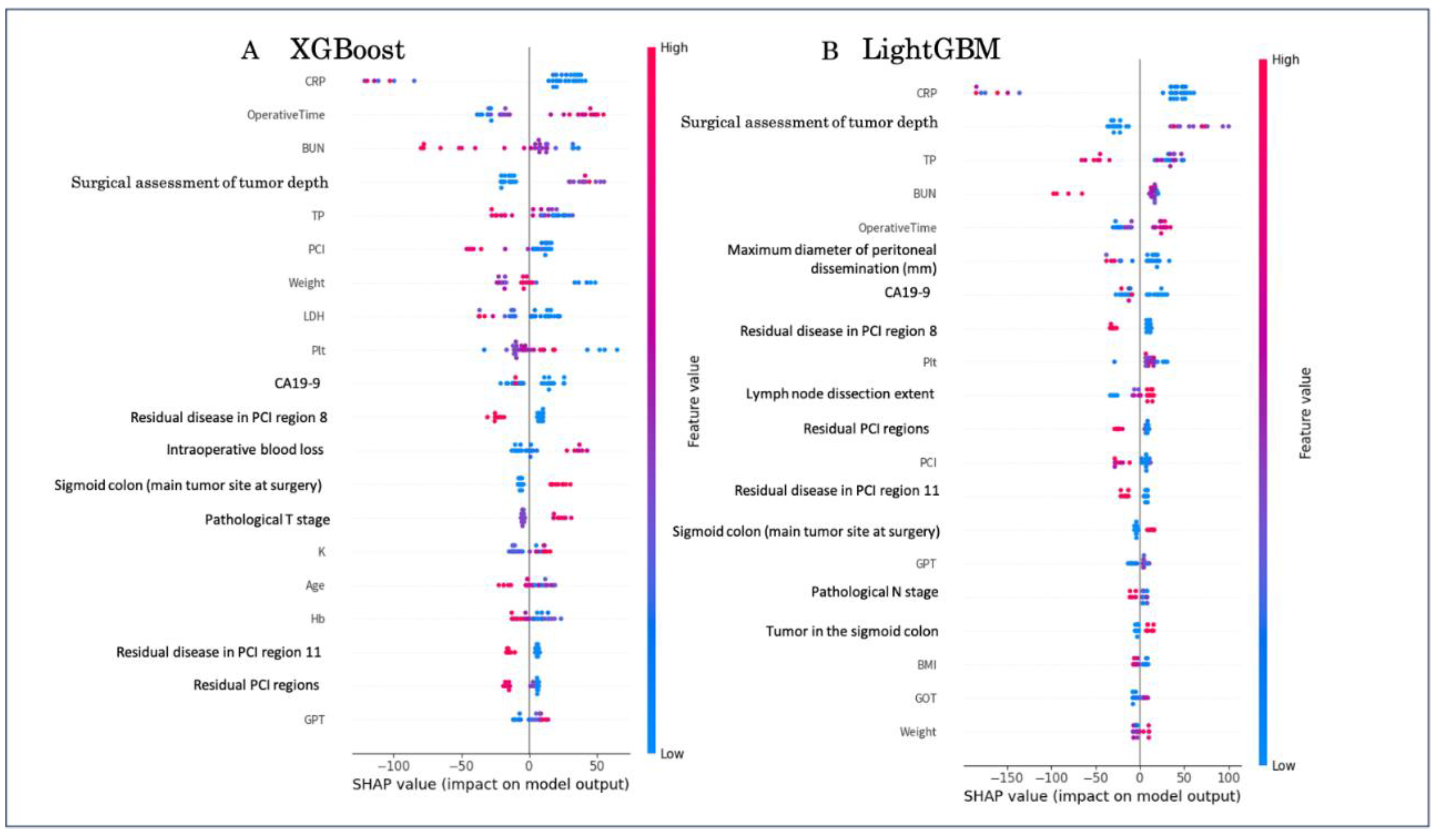
Figure 4.
LIME explanations for individual survival predictions using XGBoost models. Local explanations of three representative cases (A–C) are shown for both standard XGBoost and Optuna-tuned XGBoost models. Each bar indicates the contribution of a clinical or pathological feature to the survival prediction: green bars represent positive contributions (prolonging survival), while red bars represent negative contributions (shortening survival). Case A (491 days), Case B (506 days), and Case C (2340 days) illustrate differences in the relative importance of preoperative, intraoperative, and pathological variables between models.
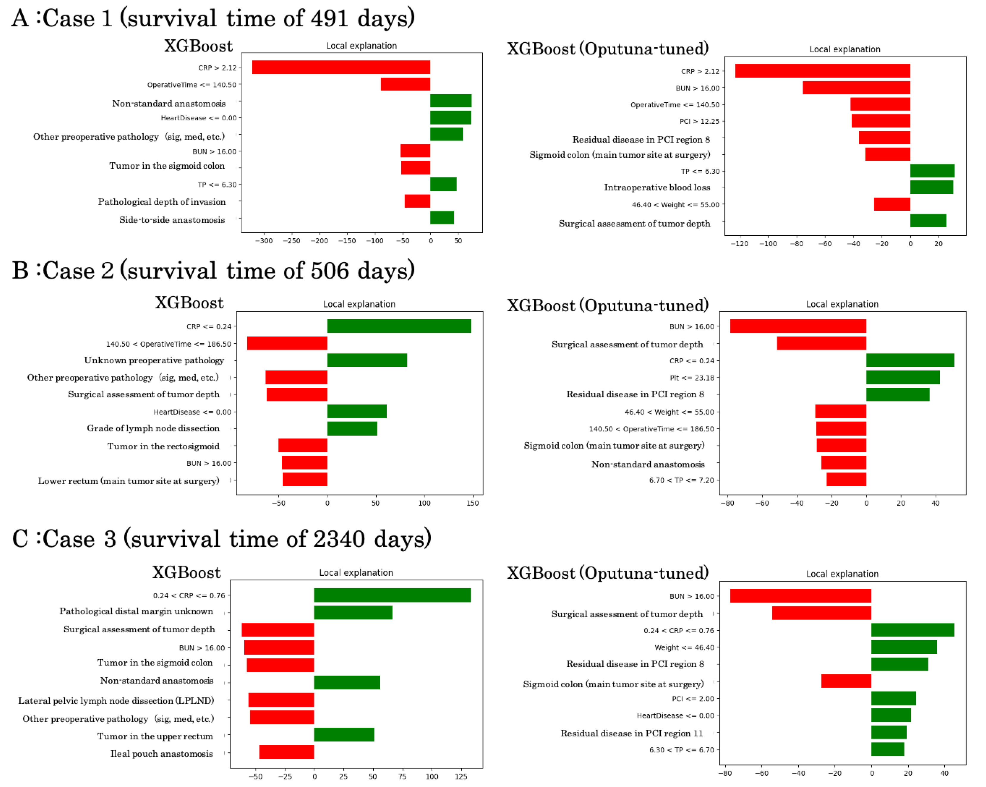

Table 1.
Variables Included in the Analysis.
| Category | Variables Included |
| Demographics & Clinical Background | Age; Sex; PS; Height; Weight; BMI; Surgery history; Comorbidities (DM, HT, heart disease, cerebrovascular disease) |
| Laboratory data | WBC; RBC; Hb; Ht; Plt; TP; Alb; T-bil; ALP; AST; ALT; LDH; BUN; Cr; Na; K; Cl; CRP; CEA; CA19-9 |
| Tumor Location | Cecum (C); Appendix (A); Transverse (T); Descending (D); Sigmoid (S); Rectosigmoid (RS); Upper rectum (Ra); Lower rectum (Rb) |
| Preoperative Treatments | Preoperative blood transfusion (BTF); Supportive treatment |
| Preoperative Pathology | Tub1; Tub2; Por; Muc; Adenosquamous; Other; Unknown |
| Operative Variables | Main tumor site; Primary site removal; Laparoscope; HIPEC; Operative time; Blood loss; Intraoperative transfusion; Residual disease; Resected organs; Lymph node dissection; Lateral pelvic lymph node dissection; ascites; anastomosis methods; surgical tumor depth; PCI (Count/ Diameter); residual PCI(Count/ Diameter); Complication (ileus, dehiscence, embolism) |
| Postoperative Pathology | Pathological TNM; lymph invasion(ly); venous invasion(v); Curability; Pathological PM/DM/RM |
| Outcomes | Overall survival (days) |
tub1, well-differentiated tubular adenocarcinoma; tub2, moderately differentiated tubular adenocarcinoma; por, poorly differentiated adenocarcinoma; muc, mucinous adenocarcinoma. PM, proximal margin; DM, distal margin; RM, radial margin.
Table 2.
:Patient Characteristics.
| Variable | n (%) or Median [range] |
| Age (years) | 66 [30–89] |
| Gender | |
| Male | 84(56) |
| Female | 66(44) |
| BMI | 20.8[9.4–40.5] |
| Comorbidity | |
| Hypertension | 39 (26.0) |
| Diabetes mellitus | 21 (14.0) |
| Heart disease | 16 (10.7) |
| Cerebrovascular disease | 6 (4.0) |
| Location of primary tumor | |
| Right colon | 79 (53) |
| Left colon | 44 (29) |
| Rectum | 27 (18) |
| Laboratory data | |
| WBC (/μL) | 6800[3000–13500] |
| Hemoglobin (g/dL) | 11.6 [5.9–16.9] |
| Platelet (×10⁴/μL) | 30.5 [6.4–71.5] |
| Albumin (g/dL) | 3.6 [1.8–4.7] |
| CRP (mg/dL) | 0.7 [0.0–25.4] |
| CEA (ng/mL) | 23.3 [0.7–15000.0] |
| CA19-9 (U/mL) | 48.5[0.4–22599.1] |
| Histologic type of primary tumor | |
| tub1 or tub2 | 110 (73) |
| Others | 36 (24) |
| Unknown | 4 (3) |
| Primary tumor resection | |
| Absent | 24 (16) |
| Present | 126 (84) |
| Operative time (min) | 191.5 [30–719] |
| Bleeding (mL) | 123.5 [0–2856] |
| Histologic type of primary tumor | |
| Well or mod | 110 (73) |
| Others | 36 (24) |
| Unknown | 4 (3) |
| Residual tumor | |
| R0 | 32 (21) |
| R1 | 5 (3) |
| R2 | 113 (75) |
| T-category | |
| T3 | 12(8) |
| T4a | 86(57) |
| T4b | 28(19) |
| Unknown | 24(16) |
| N-category | |
| N0 | 29(19) |
| N1a | 18(12) |
| N1b | 24(16) |
| N2a | 27(18) |
| N2b | 28(19) |
| Unknown | 24(16) |
| Peritoneal metastasis | |
| P1 | 30 (20) |
| P2 | 57 (38) |
| P3 | 63 (42) |
| PCI | 4 [1-29] |
| Outcome | |
| death | 121 (80.7) |
| survive | 29 (19.3) |
| Lifetime days (day; overall survival) | 635 [21–2358] |
| Median follow-up days of the surviving patients | 1364 [21-2340] |
| Median follow-up days of the dead patients | 535 [33–2358] |
Abbreviations: BMI, body mass index; WBC, white blood cell; CRP, C-reactive protein; CEA, carcinoembryonic antigen; OS, overall survival; PCI, peritoneal cancer index. Peritoneal metastasis : ;PX: Peritoneal metastasis cannot be assessed; P0: No peritoneal metastasis; P1: Metastasis localized to adjacent peritoneum; P2: Limited metastasis to distant peritoneum; P3: Diffuse metastasis to distant peritoneum.
Table 3.
:Model Performance Comparison.
| Model | MAE | RMSE | R² |
| XGBoost | 424 | 526 | 0.04 |
| LightGBM | 437 | 537 | 0.00 |
| Ridge Regression | 930 | 1250 | -4.5 |
| Lasso Regression | 1563 | 2111 | -14 |
| Linear Regression | 1561 | 2120 | -15 |
MAE = Mean Absolute Error; RMSE = Root Mean Squared Error; R² = Coefficient of Determination.
Disclaimer/Publisher’s Note: The statements, opinions and data contained in all publications are solely those of the individual author(s) and contributor(s) and not of MDPI and/or the editor(s). MDPI and/or the editor(s) disclaim responsibility for any injury to people or property resulting from any ideas, methods, instructions or products referred to in the content. |
© 2026 by the authors. Licensee MDPI, Basel, Switzerland. This article is an open access article distributed under the terms and conditions of the Creative Commons Attribution (CC BY) license.
Copyright: This open access article is published under a Creative Commons CC BY 4.0 license, which permit the free download, distribution, and reuse, provided that the author and preprint are cited in any reuse.


