Asymmetry Theory: A Unified Mathematical Framework for Classical and Relativistic Phenomena from Principle of Light-Speed Constancy

Qian Chen

doi:10.20944/preprints202601.1595.v1

Submitted:

20 January 2026

Posted:

21 January 2026

You are already at the latest version

Abstract

Asymmetry Theory (AT) is a unified mathematical framework that derives both classical and relativistic phenomena from a single empirically validated principle: light propagates at constant speed c from its emission origin. By retaining classical time and space, while introducing observer-dependent light velocity, AT bridges the conceptual divide between classical mechanics and relativistic physics, providing a common mathematical foundation that encompasses both regimes within a coherent structure.From this single principle, AT derives: (1) a light observed velocity formula explaining the Sagnac effect, GPS one-way light speed measurements, stellar aberration, and optical clock variation; (2) a unified formula encompassing both classical and relativistic Doppler effects, cosmological redshift, and Cherenkov radiation; (3) electrodynamics equations addressing particle acceleration, mass-energy equivalence, and matter waves; (4) an observer-frame formulation of Maxwell's equations that directly yields Doppler and Sagnac effects as solutions.AT reproduces all validated predictions of Special Relativity (STR) when the observer’s motion is perpendicular to the “source-observer” line, while preserving classical time synchronization and causality and naturally handling non-inertial frames.AT maintains consistency with all established empirical evidence: Michelson-Morley, optical cavity resonators, Hafele-Keating, optical clock, Ives-Stilwell spectroscopy, particle accelerators, muon decay, nuclear reactions and GPS Sagnac corrections. It also reconciles with the contested Gezari lunar ranging and Thim microwave. We demonstrate that the extensive empirical evidence traditionally cited as validating STR equally supports AT - a unified framework based on classical spacetime.To distinguish from STR, AT is empirically testable with novel predictions: (1) Sagnac phase shift Δt = 2vL/c² in inertial frame; (2) momentum asymmetry for parallel acceleration versus deceleration. A motion-controlled interferometer with first order sensitivity detecting two-way light speed deviation is proposed for the confirmative test of AT.

Keywords:

Lorentz invariance

;

Maxwell’s Equations

;

CMB

;

Sagnac effect

;

Doppler effect

;

light speed invariance

;

special relativity

;

asymmetry theory

;

time dilation

;

cosmological redshift

;

Cherenkov radiation

;

mass-energy

;

matter waves

;

stellar aberration

;

Michelson-Morley

;

twin paradox

;

Hafele-Keating

;

Ives-Stilwell

;

optical clocks

;

muon lifetime

;

lunar range test

Subject:

Physical Sciences - Theoretical Physics

I. Introduction

In 1905, Einstein introduced Special Relativity [1,2,3] with two postulates: (1) principle of relativity and (2) principle of the constancy of the velocity of light, which stated: “in empty space, light is always propagated with a definite velocity V which is independent of the state of motion of the emitting body”. The second postulate has extensive empirical support: binary x-ray pulsar Her X1 timing signatures [8], gamma rays from fast pions [11], and moving optical element experiments [12] all confirm that light speed does not depend on source velocity. However, the additional derived from principle of relativity - that light speed is also independent of the observer’s motion, has not been conclusively proven. All current tests can only provide an upper limit. The traditional Michelson-Morley interferometers [7,43] merely confirmed an upper limit of about 1km/s. Modern optical cavity resonators [44,45] claim higher precision but involve confined light with potential “dragging” effects that complicate interpretation. Some contested measurements [26,27,39], including lunar laser ranging and GPS-based tests, have reported results that appear inconsistent with strict light speed invariance for all observers. Additionally, phenomena like the Sagnac effect [15,16,17] in rotating frames, CMB dipolar asymmetry [47], and Doppler anisotropy [37] suggest observer-dependent light speed variations.

These observations motivate a fundamental question: Is Einstein’s postulate of relativity—necessary to explain relativistic phenomena? Or can these phenomena be derived from only the empirically validated principle of light speed constancy, with classical time and space? Previous attempts with classical principles include the ether theory (Lorentz 1904 [6]), which relies on the existence of ether, and the emission theory (Ritz 1908 [9]), which contradicts the principle of constant light speed [10].

Asymmetry Theory Framework

This paper presents Asymmetry Theory (AT), a mathematically rigorous framework that demonstrates: all validated relativistic predictions can be derived from the single empirically validated principle of light speed constancy with classical spacetime. Define an emission event

(S (t_{s}), t_{s})

of a photon

L

, the principle of light-speed constancy is be represented as:

L (t) - S (t_{s}) = c (t - t_{s}) (Base Equation)

All results are derived from this base equation through strict mathematics, which are summarized in Table 1 step by step with supporting empirical evidence, and collectively termed as the “Asymmetry Theory” [23,24,25,35,40]. AT is based on the relations between light events, without the assumptions like the ether or universal preferred frames.

Relationship to Lorentz transformation & STR

By writing the base equation in spacetime format, we mathematically prove that when observer motion is perpendicular to the source-observer line, AT equation takes the same spatial form as LT with Lorentz factor γ. This explains why AT reproduces all validated STR predictions in this case. However, the crucial distinction is that time never varies in AT, which derives clock variations as physical effects of clock measurement. This preserves classical time synchronization and causality, naturally eliminating temporal paradoxes like the twin paradox while maintaining empirical agreement with experiments like Hafele-Keating [29] and muon decay [31]. A detailed comparison between AT and STR is summarized in Table 2.

Distinguishing key concepts

To understand how AT maintains the light speed invariance principle, it is fundamental to distinguish the constant light propagation velocity, defined as the relative velocity between photon

L (t)

and light origin

S (t_{s})

, from the light observed velocity, defined as the relative velocity between

L (t)

and observer

O (t) .

To understand AT’s reconciliation of absolute time with experimental clock variations, it is essential to distinguish classical time t from optical/atomic clocks which are based on photon oscillations.

Scope of Derivations

From the single base equation, AT derives:

1. Light velocity formula: Observer-dependent observed light speed, explaining Sagnac effect [15,16], stellar aberration, Michelson-Morley[7], optical clock variations [28], and GPS [39].

2. The “time scaling factor”

d t_{o} / d t_{s}

mathematically describes how moving observers perceive clock variations and resolves twin paradox.

3. Unified Doppler/redshift formula: Formulas encompassing classical Doppler effect [37], relativistic Doppler [30,36], cosmological redshift [21], and Cherenkov radiation [34], all linked through the time scaling factor

d t_{o} / d t_{s}

. Extends to time-varying velocities (novel). Predicts no frequency shift for circular motion, confirmed by experiments [13,14]. A single equation covers all scenarios of relativistic Doppler effect, explaining Ives-Stilwell experiments [30,36].

3. Electrodynamics: Mass-energy equivalence and relativistic momentum, explaining particle accelerators [32] and nuclear reactions [33]; Novel prediction of momentum anisotropy; Formula linking mass-energy to de Broglie wavelength [41], suggesting potential quantum unification pathway.

4. Maxwell’s equations: Observer-frame formulation for moving observers [40] that directly yields Doppler and Sagnac effects and preserves classical velocity addition, eliminating the need for modified Galilean electrodynamics (GED). Demonstrates invariance of Lorentz force across observer frames (Barnett [18]).

Novel testable predictions and experiment design

AT also made novel testable predictions that distinguish from STR, including generalized Sagnac effect in inertial frames and asymmetric momentum-to-acceleration ratios.

A first-order sensitive interferometer capable of detecting two-way light speed deviation by a lab-controlled motion of 0.1m/s is designed in [46] for a conclusive test of light speed invariance to moving observers.

Paper Organization

Section II derives the light velocity formulas. Section III presents empirical evidence and explanations. Section IV derives the unified Doppler/redshift formulas. Section V presents the generalized Maxwell’s equations. Section VI derives electrodynamic formulas. Section VII shows STR as a special case. Section VIII discusses theoretical progress. Section IX presents predictions and experimental proposals. Section X provides discussion and conclusions.

Summary

Asymmetry Theory is mathematically rigorous and supported by all empirical evidence. It unifies classical and relativistic physical phenomena across fields like atomics, optics, electromagnetics and quantum. By demonstrating that relativistic phenomena can be derived from classical spacetime. AT preserves time synchronization and causality, avoids temporal paradoxes, reproduces all validated STR predictions, extends naturally to non-inertial frames, and makes clear testable predictions distinguishing it from STR. Whether AT or STR provides the more fundamental description of nature is an empirical question—to be answered through the proposed experiments.

Table I. Summary of AT framework derivation from the base equation and supporting Empirical evidence.

Physical principle	Mathematical Derivation of formulas	Empirical support
Light velocity constancy	$L (t) - S (t_{s}) = c (t - t_{s})$	Base equation
1. Light velocity	$b a s e \Rightarrow c_{so} (t) = c - v_{o} (t)$	Her X1 [8], Fast pion [11]
1.1 One way light speed	$1. \Rightarrow c_{so} = \|c - v_{o}\|$	GPS measurement [39]
1.2 Generalized Sagnac effect	$1.1 \Rightarrow Δ t \approx 2 v L / c^{2}$	Sagnac effect [15,16]
1.3 Stellar aberration	$1. \Rightarrow \sin (θ_{o} - ϕ) = v_{o} / c \sin (ϕ)$	Stellar aberration
1.4 Two-way light speed	$1.1 \Rightarrow c_{s o r} = c * (1 - v_{o}^{2} / c^{2})$	M-M interferometer [7] Cavity Resonator [44,45]
1.5 Two-way moving reflector	$1.1 \Rightarrow c_{s o r} \approx c + v_{r}$	Lunar range light speed [27]
1.6 $v_{o}$ perpendicular to observer line $\vec{S (t_{s}) O (t_{s})}$	$1. \Rightarrow c_{s o} = c * \sqrt{1 - v_{o}^{2} / c^{2}}$	Lorentz factor
1.7 Optical Clock time dilation	$1.6 \Rightarrow f / f_{0} = c_{s o} / c = \sqrt{1 - v_{o}^{2} / c^{2}}$	Hafele-Keating [28], Optical clock [29], muon decay [31]
2. Electrodynamics
2.1 Particle acceleration	$1. \Rightarrow Δ P / c * \|c - v_{o}\| = m * Δ v_{o}$	Kaufmann [32]
2.2 Mass energy relationship	$2.1 \Rightarrow Δ E = Δ m * c^{2}$	Nuclear reaction [33]
2.3 Matter waves relationship	$2.1 & 2.2 \Rightarrow Δ E = h * c / λ$	De Broglie matter waves
3. Unified Doppler/redshift	$b a s e \Rightarrow O (t_{o}) - S (t_{s}) = c (t_{o} - t_{s})$	Classical velocity addition
3.1 Time dilation factor	$3. \Rightarrow \frac{d t_{o}}{d t_{s}} = \frac{c - v_{s} (t_{s}) \cos (θ_{s})}{c + v_{o} (t_{o}) \cos (θ_{o})}$	Resolves Twin Paradox
3.2 Traditional Doppler effect	$3.1 \Rightarrow \frac{f_{s} (t_{s})}{f_{o} (t_{o})} = \frac{c - v_{s} (t_{s}) \cos (θ_{s})}{c + v_{o} (t_{o}) \cos (θ_{o})}$	Rotational microwave [14]
3.3 Relativistic Doppler effect	$3.2 & 1.6 \Rightarrow \frac{f_{s} (t_{s})}{f_{o} (t_{o})} = \frac{c - v_{s} c o s θ_{s}}{c + v_{o} c o s θ_{o}} \frac{\sqrt{1 - v_{o}^{2} / c^{2}}}{\sqrt{1 - v_{s}^{2} / c^{2}}}$	Ives-Stilwell [30,36] (covers all scenarios in STR)
3.4 Cosmological redshift	$3. \Rightarrow \frac{f_{s} (t_{s})}{f_{o} (t_{o})} = \frac{c / a (t_{s}) - v_{s} (t_{s}) \cos (θ_{s})}{c / a (t_{o}) + v_{o} (t_{o}) \cos (θ_{o})}$	Cosmological redshift [21]
3.5 Cherenkov emission angle	$3. \Rightarrow \cos (θ_{e}) = c / n * v_{p}$	Cherenkov radiation [34]
4. Maxwell’s equations	$3.1 \Rightarrow \nabla^{2} E - \frac{1}{{(c - v_{o})}^{2}} \frac{\partial^{2}}{\partial {t_{o}}^{2}} E = 0$	Equivalent with original form Doppler and Sagnac effects

II. Light Velocity

This section establishes the mathematical foundation of Asymmetry Theory by deriving light velocity formulas from the single principle of light speed constancy.

A.: Foundation: Light Origin and Base Equation

Let a photon

L

be emitted at the spacetime event

E_{s} \equiv (S (t_{s}), t_{s}), S \in ℝ^{3}, t_{s} \in ℝ,

where

S (t_{s})

is the spatial position of the emitter at emission time

t_{s}

, which defines the light origin for that photon. The fundamental principle governing light propagation is:

Principle 1: In empty space, the light always propagates with a velocity

c

. independent of the state of motion of the emitting body [1].

Let

L (t) \in ℝ^{3}

be the photon’s trajectory, we have:

L (t) - S (t_{s}) = c (t - t_{s}), t \geq t_{s},

(1)

where

c

is the photon propagation velocity, see Figure 1. This relation (1) expresses one-way propagation invariance of photon relative to the origin event, which makes no assumption of the ether, an universal preferred frame or clock synchronization.

**Note:

S (t_{s})

differs from the emitter’s position; they match at

t_{s}

but are independent after emission, t>

t_{s}

.

Now, let a photon be observed at the spacetime event

E_{o} \equiv (O (t_{o}), t_{o}), O \in ℝ^{3}, t_{o} \in ℝ,

where

O (t_{o})

is the spatial position of an observer

O

detecting the photon at time

t_{o}

, which means:

O (t_{o}) = L (t_{o})

Combining with Eq. (1), we have:

O (t_{o}) - S (t_{s}) = c (t_{o} - t_{s})

(2)

All results in this paper are mathematically derived from Eq. (1) without additional postulates.

B.: Propagation Velocity vs. Observed Velocity

It is fundamental to distinguish between two velocities:

Define the light propagation velocity

c_{p r o} (t)

as the relative velocity between photon

L (t)

and light origin

S (t_{s}) :

c_{p r o} (t) = \frac{d}{d t} (L (t) - S (t_{s}))

(3)

Define the light observed velocity

c_{so} (t)

as the relative velocity between photon

L (t)

and observer

O (t) :

c_{so} (t) = \frac{d}{d t} (L (t) - O (t))

(4)

Note: This distinction is analogous to the propagation frequency vs. observed frequency in Doppler effect.

Theorem 1: The light propagation velocity is always

c

.

Proof: Combining Eq. (1) and Eq. (3), we have:

c_{p r o} (t) = \frac{d}{d t} (c (t - t_{s})) = c . ■

Now define

v_{o} (t)

as the velocity of observer

O

relative to

S (t_{s})

and

v_{s} (t)

as the velocity of the light source relative to

S (t_{s})

(see Figure 1 for illustration). By definition:

v_{o} (t) = \frac{d}{d t} (O (t) - S (t_{s}))

Theorem 2: The observed velocity of a light emitted from

S (t_{s})

as to an observer

O

is

c_{so} (t) = c - v_{o} (t)

(5)

Proof: From definition, we have:

c_{so} (t) = \frac{d}{d t} (L (t) - O (t)) = \frac{d}{d t} (L (t) - S (t_{s})) - \frac{d}{d t} (O (t) - S (t_{s})) = c_{p r o} (t) - v_{o} (t) = c - v_{o} (t) . ■

In summary,

Light propagation velocity $c_{p r o} (t)$ is always $c$

**Note: Hence, by default throughout the paper, “light velocity” refers to the observed velocity $c_{so} (t)$ .
Light observed velocity $c_{so} (t)$ as to an observer $O$ depends on its velocity, specifically, $c - v_{o} (t)$
If $v_{o} (t) = 0$ , $c_{so} (t)$ is $c$

C.: Composition of Velocity/Galilean transformation

Assuming two observers

O

and

O^{'}

with velocity of

v_{o} (t)

and

v_{o^{'}} (t)

respectively, which follows:

v_{o^{'}} (t) - v_{o} (t) = v

Let

c_{so} (t)

and

c_{s o'} (t)

be the light observed velocity of

O

and

O^{'}

. From (5), we have:

c_{s o'} (t) = c - v_{o^{'}} (t) = c - v_{o} (t) - v = c_{so} (t) - v

(6)

Hence, Asymmetry Theory maintains the classical addition of velocity across different observers.

D.: Lorentz Transformation and STR

Let

F (x, y, z)

be an inertial frame with the light origin

S

at rest in the origin. We can rewrite Eq. (1) as spacetime form:

x^{2} + y^{2} + z^{2} - c^{2} t^{2} = 0

(7)

The plot of (7) is the well-known light cone.

Let

F^{'} (x', y', z')

be an observer

O

’s inertial frame moving relative to

F

with velocity

v_{o}

, Eq. (7) becomes:

{(x^{'} - v_{o x} t)}^{2} + {(y^{'} - v_{o y} t)}^{2} + {(z^{'} - v_{o z} t)}^{2} - c^{2} t^{2} = 0

(8)

Eq. (8) is equivalent to Eq. (2) of AT from the perspective of observer

O

. As an example, Figure. 2(a) depicts the light cone of (8) when

v_{o}

is

c

/2 in X direction, which is asymmetric/anisotropic.

When

v_{o}

is perpendicular to the “source-observer” line

(x^{'}, y^{'}, z^{'})

, Eq. (8) becomes:

{x^{'}}^{2} + {y^{'}}^{2} + {z^{'}}^{2} + {v_{o}}^{2} t^{2} - c^{2} t^{2} = 0

{x^{'}}^{2} + {y^{'}}^{2} + {z^{'}}^{2} - \frac{1}{γ^{2}} c^{2} {t^{'}}^{2} = 0

(9)

where

γ

is the Lorentz factor and

t^{'} = t .

Hence, in this specific case, AT shares the same form as LT, i.e. STR. Figure 2(b) depicts the light cone, which becomes symmetric just like LT

E.: Time sync. and Causality

Although AT’s Eq. (9) shares the same form as LT/STR, the crucial distinction is that in Asymmetry Theory, time is absolute

t^{'} = t

; instead, the observed speed of light becomes

c / γ

to maintain LT equation. As a result, AT maintains classical time synchronization and event causality.

STR [1] claims that time synchronization is impossible. Let a ray of light start at the “A time”

t_{A}

from A towards B, let it at the “B time”

t_{B}

be reflected at B in the direction of A, and arrive again at A at the “A time”

t_{A}^{,}

STR defines the two clocks synchronized if

t_{B} - t_{A} = t_{A}^{,} - t_{B}

However, for an observer moving with speed

v

, we have

t_{B} - t_{A} = \frac{r_{A B}}{c - v}, t_{A}^{,} - t_{B} = \frac{r_{A B}}{c + v}

(10)

STR cannot resolve this contradiction and subsequently asserts that the clocks at A and B are not synchronized [1].

By contrast, Asymmetry Theory yields:

(t_{B} - t_{A}) - (t_{A}^{,} - t_{B}) = 2 v * r_{A B} / (c^{2} - v^{2})

(11)

which is exactly same formula as Sagnac effect [16]. Thus, AT avoids contradiction in (10) and instead predicts a generalized Sagnac effect as (11) for nonrotational frames, which can be experimentally validated with a novel M-M type interferometer in [46].

F.: “Time Dilation”: Absolute Time vs. Physical Clock

Theorem 3: If the observer’s velocity is constant

v_{o}

and perpendicular to

\vec{S (t_{s}) O (t_{s})}

, the light observed speed

c_{s o}

is:

c_{s o} = c / γ

(12)

Proof: From (5), we have:

c_{s o} = |c - v_{o}| = \sqrt{c^{2} + v_{o}^{2} - 2 c v_{o} c o s (π - θ_{s})}

Since

ϕ = 90^{°}

(see Figure 1.), thus

c o s (π - θ_{s}) = v_{o} / c

c_{s o} = c * \sqrt{1 - v_{o}^{2} / c^{2}} = c / γ ■

This result can also be derived directly from Eq. (11). Hence, the Lorentz factor

γ

is mathematically derived since AT shares the same form of Lorentz equation in this case.

A critical point to understand “Time dilation”: AT distinguishes between time itself and physical clock.

Absolute Time t: Universal coordinate, same for all observers, never varies

Physical Clocks (Atomic/Optical): Devices measuring time based on photon oscillations

Optical/Atomic clocks measure time by counting the oscillations of photon. We have a relationship between light speed and frequency as:

c = f * λ

, where

λ

is the wavelength. Let

f (v_{o})

be the frequency of a moving clock with the observer speed

v_{o}

, we have:

c_{s o} = f (v_{o}) * λ and c = f (0) * λ

From Eq. (12), when an optical clock moves with velocity

v_{o}

perpendicular to its measurement axis (typical geometry):

c_{s o} = c / γ \Rightarrow \frac{f (v_{o})}{f (0)} = \frac{c_{s o}}{c} = \frac{1}{γ}

(13)

In summary, a moving clock physically ticks slower by factor

γ

—not because time has changed, but because the electromagnetic process driving the clock is affected by motion. It mathematically explains the “Time Dilation”: Optical clocks [28], Muon lifetime (muons are “clocks” based on EM interactions) [31] and Hafele-Keating [29].

III. Empirical Evidence

A.: One-way light speed & GPS measurement

AT’s light velocity formula (5) directly explains why one-way light speed measurement yield values different from c.

From Eq. (5), the light observed speed

c_{so} (t) \in ℝ

is:

c_{so} (t) = |c - v_{o} (t)|

. when

v_{o} (t)

is constant

v_{o}

, it becomes:

c_{so} = |c - v_{o}|

.

c_{so}

equals to the one-way measured light speed, which aligns with the GPS light speed measurement like [39].

STR argues that measuring one-way light speed is impossible due to clock synchronization errors. AT shows it is measurable and Sagnac effect is its direct result. In fact, GPS is a good example of one-way light speed application with clock synchronization. The ground observers have velocity

v_{o}

in the Earth-Centered Inertial (ECI) frame. Hence, the one-way light speed is

c_{so} = |c - v_{o}|

. Current GPS must apply “Sagnac correction” to correct the timing error caused by using c as the light speed. AT explains this directly and no Sagnac correction is necessary since it is a direct inference from AT’s light formula.

B.: Round-trip light speed & M-M interferometer

Theorem 4: The round-trip speed of light

c_{s o r}

from

S (t_{s})

to

O

with velocity

v_{o}

along the light path (static reflector):

c_{s o r} = c * (1 - v_{o}^{2} / c^{2})

(14)

Proof: The round-trip speed is the average of the forward and backward speeds. From (5), we have

c_{s o r} = \frac{2}{\frac{1}{c - v_{o}} + \frac{1}{c + v_{o}}} = c * (1 - \frac{v_{o}^{2}}{c^{2}}) ■

In summary, the round-trip light speed

c_{s o r} \approx c

if

v_{o} ≪ c

.

Explanation of Michelson Morley [7,43]:

If we assume the ECI frame, for Earth’s rotation,

v_{o} = 460 m / s

. From (14), we have:

Δ c = v_{o}^{2} / c \approx 0.7 m m / s

which is below the detection threshold of traditional Michelson-Morley interferometer. Hence, the result is null. For a further test, a novel first-order sensitive M-M type interferometer is designed in [46] which can detect two-way light speed deviation caused by a lab induced motion as small as 0.1m/s.

C.: Modern Cavity Resonator Experiment

The modern M-M experiments [44,45] measure the frequency difference between cavity resonators with sensitivity better than 10⁻¹⁵.

AT Explanation:

When light resonates inside a cavity, the cavity walls effectively “re-emit” photons continuously. The light appears “sticking” to the cavity: If we turn the resonator, the light inside will turn correspondingly. Hence, the confined cavity light is different from the light in free space interferometer and may use a different emission origin.

The hypothesis is the emission origin may be the cavity frame itself i.e.

v_{o}

=0. From (14) we have

c_{s o r} = c

, which explains the null result. Again, the first order interferometer in [46] will provide a further confirmative test.

D.: Round-trip light speed with moving reflector

The contested Lunar laser ranging test (Gezari, 2009 [27]) measures the round-trip light speed at

c

+200m/s, in which the observatory moves along the line-of-sight of the reflector in moon at 200m/s due to the earth rotation.

AT Explanation:

Let the observatory

O

velocities to the light origin and reflector be

v_{o}

and

v_{r}

. So, the reflector velocity to the origin is

v_{o} - v_{r} .

From (5), the round-trip speed

c_{s o r}

is:

c_{s o r} = \frac{2}{\frac{1}{c - (v_{o} - v_{r})} + \frac{1 - v_{r} / (c - (v_{o} - v_{r}))}{c + v_{o}}}

= c (1 - v_{o}^{2} / c^{2}) + v_{r} (1 + v_{o} / c) \approx c + v_{r}

(15)

We can also derive (15) from the composition of velocity (6). Imagine an

O^{'}

static with the reflector, thus its velocity relative to

O

is

- v_{r}

. From (6) and (15):

c_{s o r} = c (1 - v_{o}^{2} / c^{2}) - (- v_{r}) \approx c + v_{r}

(16)

In Lunar ranging:

v_{r} = 200 m / s

, we have:

c_{s o r} = c

+200m/s, which matches the result perfectly. While the Lunar laser range test is contested as anomalous in STR but follows naturally from AT.

E.: Generalized Sagnac Effect

The Sagnac effect [15] shows that two light beams, sent clockwise and counterclockwise around a closed path, take different time to travel the path, which contradicted the assumption that the light velocity is independent of the motion of the observer. STR attributed this contradiction to the rotating/accelerating frame [4,17]. The Sagnac effect can be extended to a FOG [16] with

Δ t = 2 v L / c^{2}

, where

v

is the speed of the detector,

L

is the length of the path.

Let

v_{o}^{+}

,

v_{o}^{-}

be the velocities of the detector to the origins of two light beams, then

v_{o}^{+} - v_{o}^{-} = 2 v

. According to (5), the light velocities as measured by the detector are

c - v_{o}^{+}

and

c - v_{o}^{-},

respectively. Therefore,

Δ t = \frac{L}{c - v_{o}^{+}} - \frac{L}{c - v_{o}^{-}} = \frac{2 v L}{(c - v_{o}^{-}) (c - v_{o}^{+})} \approx \frac{2 v L}{c^{2}}

(17)

In summary, AT predicts the generalized Sagnac effect as a direct inference of the light velocity formula (5) as the result of light velocity anisotropy, which applies to non-rotational frames and resolves the time synchronization problem (10) in STR. Thus, the GPS “Sagnac correction” is not necessary if formula (5) is applied. This prediction can be experimentally validated with a novel M-M type interferometer in [46].

F.: Key angles and stellar aberration

Aberration of starlight is a phenomenon of difference in the observed angle of starlight due to the velocity of the observer. Figure 1 shows key angles for the light velocity,

θ_{s}, θ_{o}, ϕ

. The stellar aberration is

θ_{o} - ϕ

. Assuming

v_{o} (t)

is constant

v_{o}

, the relationship is determined from Figure 1:

\sin (θ_{o} - ϕ) = \frac{v_{o}}{c} \sin (ϕ)

(18)

When

ϕ = 90^{°}

, we have

\cos (θ_{o}) = - v_{o} / c

, which is the same as STR in [1], noting

θ_{o}

is

ψ^{'}

.

IV. Unification of Doppler Effect

From the single Eq. (2), AT derives a unified framework for frequency shifts observed when sources and/or observers are in motion. We show that classical Doppler effect, relativistic Doppler effect, cosmological redshift, and Cherenkov radiation angle all emerge from a single mathematical formalism—the time scaling factor. This unification provides compelling evidence for AT’s foundational principles.

A.: Time Scaling Factor and Observed Time

The foundation of observed light frequency shifts is the time scaling factor, defined as

d t_{o} / d t_{s}

. A light wave can be viewed as continuous emission events

(S (t_{s}), t_{s})

and the corresponding observed events

(O (t_{o}), t_{o})

. From (2),

O (t_{o}) - S (t_{s}) = c (t_{o} - t_{s})

Perform an inner product of both sides, we have:

(O (t_{o}) - S (t_{s})) • (O (t_{o}) - S (t_{s})) = c^{2} {(t_{o} - t_{s})}^{2}

Differentiate both sides as to

t_{s}

and reorganize:

\frac{(O (t_{o}) - S (t_{s}))}{c (t_{o} - t_{s})} • (v_{o} (t_{o}) \frac{d t_{o}}{d t_{s}} - v_{s} (t_{s})) = c (\frac{d t_{o}}{d t_{s}} - 1)

Let

i_{o s}

denote the unit vector in

\vec{S (t_{s}) O (t_{s})}

, we have:

i_{o s} • v_{o} (t_{o}) \frac{d t_{o}}{d t_{s}} - i_{o s} • v_{s} (t_{s}) = c (\frac{d t_{o}}{d t_{s}} - 1)

Finally, the formula for time scaling factor is:

\frac{d t_{o}}{d t_{s}} = \frac{c - v_{s} (t_{s}) \cos (θ_{s})}{c + v_{o} (t_{o}) \cos (θ_{o})}

(19)

When

v_{o} (t), v_{s} (t)

are constant

v_{o}, v_{s}

and

θ_{s} = 0, θ_{o} = π

, (19) reduces to:

\frac{d t_{o}}{d t_{s}} = \frac{c - v_{s}}{c - v_{o}}

(20)

To understand the physical meaning of “time scaling factor”, let’s consider the phenomenon of a moving observer watches a static clock ticking.

When $v_{o} >$ 0 (moving away from clock): $d t_{o} / d t_{s}$ 1, the clock appears to run slower.
When $v_{o} <$ 0 (moving toward clock): $d t_{o} / d t_{s} < 1$ , the clock appears to run faster.
When $v_{o} \to c$ (approaching light speed): $d t_{o} / d t_{s} \to \infty$ , clock appears to stop.

Hence, “time scaling factor” describes how the motions of the observer/emitter impact the observed time. STR tried to use the same phenomenon to explain “time dilation”. But since “dilation” means the clock always runs slower, STR can’t explain the scenario when clock runs faster. It’s important to note that the actual time never varies in AT, just like the physical clock here doesn’t run faster or slower. What varies here is the observed clock time. Hence, AT naturally avoids “twin paradox” when using actual time.

Now consider the “twin paradox” based on the observed times:

t_{s}

and

t_{o}

. Assume a light source is at rest and an observer moves away from the same position and returns. Each records its time as

t_{s}

and

t_{o}

, with the start time

0

, and the return times as

t_{s} = t_{1}

and

t_{o} = t_{1} ’

.

In Appendix. A, we mathematically proved that

t_{1} = t_{1} ’

, which means the elapsed times measured by

t_{s}

and

t_{o}

are always the same independent of the movement. Hence, both twins will experience same observed time and there is no “twin paradox”. Note: The impact on moving optical/atomic clock (13) is not considered in this case, which explains Hafele-Keating [29].

B.: Derivation of classical Doppler Effect

The classical Doppler effect describes frequency shifts between the light wave emitted frequency and the observed frequency without the relativistic clock effects.

Theorem 5: For a light source emitting at frequency

f_{s} (t_{s})

, the observed frequency

f_{o} (t_{o})

satisfies the following formula:

\frac{f_{s} (t_{s})}{f_{o} (t_{o})} = \frac{c - v_{s} (t_{s}) \cos (θ_{s})}{c + v_{o} (t_{o}) \cos (θ_{o})}

(21)

Proof: Because the total wave-number emitted during the period

{dt}_{s}

should be equal to that received during the period

{dt}_{o}

, we have

f_{o} (t_{o}) * d t_{o} = f_{s} (t_{s}) * d t_{s}

\Rightarrow \frac{f_{s} (t_{s})}{f_{o} (t_{o})} = \frac{d t_{o}}{d t_{s}}

Replaces with (19), we have (21) derived.

■

Traditionally, Doppler effect formulas are limited for constant velocity. AT’s formula extends to time-varying velocity, a theoretical breakthrough. Assuming constant velocities

v_{o}, v_{s}

and

θ_{s} = 0, θ_{o} = π

, this general formula (21) reduce to the standard Doppler Effect formula [20]:

\frac{f_{s}}{f_{o}} = \frac{c - v_{s}}{c - v_{o}}

C.: Derivation of Relativistic Doppler Effect

When the source or observer is an atomic/optical clock, we must account for the clock’s internal frequency change due to motion from Eq. (13), which is demonstrated in the Ives–Stilwell experiments [30,36].

Theorem 6: For atomic clocks as sources/observers, the Doppler effect formula is:

\frac{f_{s} (t_{s})}{f_{o} (t_{o})} = \frac{c - v_{s} (t_{s}) c o s θ_{s}}{c + v_{o} (t_{o}) c o s θ_{o}} * \frac{\sqrt{1 - v_{o}^{2} (t_{o}) / c^{2}}}{\sqrt{1 - v_{s}^{2} (t_{s}) / c^{2}}}

(22)

Proof: Note that

f_{s} (t_{s})

and

f_{o} (t_{o})

are the frequencies at rest. From (13), the emitted frequency and observed frequency with the frequency change due to motion will be:

f_{s} (t_{s}) \sqrt{1 - v_{s}^{2} (t_{s}) / c^{2}} and f_{o} (t_{o}) \sqrt{1 - v_{o}^{2} (t_{o}) / c^{2}}

.

Apply (21), we have:

\frac{f_{s} (t_{s}) \sqrt{1 - v_{s}^{2} (t_{s}) / c^{2}}}{f_{o} (t_{o}) \sqrt{1 - v_{o}^{2} (t_{o}) / c^{2}}} = \frac{c - v_{s} (t_{s}) c o s θ_{s}}{c + v_{o} (t_{o}) c o s θ_{o}}

which follows the formula (22).

■

In STR, different formulas are required for the relativistic Doppler effect in different scenarios. Table II. shows this single formula (22) covers all scenarios, compelling evidence for its validity.

D.: Thim rotational microwave & Ives-Stilwell

The Thim experiment [14] finds no frequency shift for rotational microwave devices, which is contended to contradict STR [19].

AT Explanation: Since microwave devices are not optical/atomic clocks, the classical Doppler effect formula (21) is applied. For circular motion, we have

θ_{s} = θ_{o} = 90^{o}

, from (21), we have:

f_{s} (t_{s}) / f_{o} (t_{o}) = 1

i.e. no frequency shift, which aligns with Thim’s result.

The Ives-Stilwell spectroscopy experiments [30,36] measured Doppler shifts from high-speed ions and results matched relativistic Doppler predictions.

AT Explanation: Fast-moving ions are atomic systems (atomic clocks). Eq. (22) is applied. In a rotation,

θ_{s} = θ_{o} = 90^{o}

, if we assume

v_{o} = 0,

(22) reduces to:

\frac{f_{s}}{f_{o}} = \frac{\sqrt{1 - v_{s} / c}}{\sqrt{1 + v_{s} / c}}

(23)

a standard relativistic Doppler effect aligned with the result.

AT mathematically explains both the results of Thim and Ives-Stilwell by distinguishing the atomic clocks from non-atomic devices, which is a further proof of AT’s concept that the relativistic clock effect is a change of physical oscillation not the actual time.

E.: Derivation of Cosmological red-shift formula

Cosmological red-shift [21] is traditionally believed to be unrelated to the Doppler Effect. AT shows that it can be mathematically derived from the time scaling factor.

The cosmological red-shift formula is:

\frac{f_{s} (t_{s})}{f_{o} (t_{o})} = \frac{a (t_{o})}{a (t_{s})}

(24)

where

a (t)

is the cosmic scale factor. Under the assumption of inflating Universe, equation (2) becomes:

O (t_{o}) - S (t_{s}) = \int_{t_{s}}^{t_{o}} c / a (t) d t

Following the similar mathematical derivation of

d t_{o} / d t_{s}

in A. of this section, we derived the following formula in [24]:

\frac{f_{s} (t_{s})}{f_{o} (t_{o})} = \frac{c / a (t_{s}) - v_{s} (t_{s}) \cos (θ_{s})}{c / a (t_{o}) + v_{o} (t_{o}) \cos (θ_{o})}

(25)

When

v_{s} (t_{s}), v_{o} (t_{o}) ≪ c

, (25) becomes:

\frac{f_{s} (t_{s})}{f_{o} (t_{o})} \approx \frac{a (t_{o})}{a (t_{s})}

which is the same as (24).

Hence, cosmological redshift emerges naturally from the same time scaling factor framework in AT, which can be viewed as Doppler effect in expanding spacetime.

F.: Derivation of Cherenkov radiation emission angle

Cherenkov radiation [34] is electromagnetic radiation emitted when a charged particle passes through a dielectric medium at a speed greater than the light speed in that medium. It has a key emission angle

θ_{e}

determined by:

\cos (θ_{e}) = \frac{c}{n} / v_{p}

(26)

where

v_{p}

is the particle speed and

n

is the refractive index.

Let’s start derivation from (19). In this case, we have:

\frac{d t_{o}}{d t_{s}} = (\frac{c}{n} - v_{p} \cos (θ_{e})) / \frac{c}{n}

(27)

Now according to Fermat’s principle, the light path should take the minimum time to the observer. We have:

d t_{o} / d t_{s} = 0

Substitute to (27), we get the same formula as (26):

\cos (θ_{e}) = (c / n) / v_{p}

The Cherenkov radiation angle emerges from the same time scaling factor combined with Fermat’s principle. Again, a seemingly distinct phenomenon unifies under the AT framework.

V.: Maxwell Equations

This section addresses a critical question: How do Maxwell’s equations, which describe electromagnetic phenomena, relate to AT? We show that an observer-frame formulation of the standard equations naturally accounts for observer motion, which directly yields the light velocity formula (Eq. 5), Doppler effect (Eq. 21), and Sagnac effect (Eq. 8) as solutions—providing independent confirmation of AT’s core results. We also show that the Lorentz force formula is invariant when properly formulated and classical velocity addition applies to different observers, eliminating the need for modified Galilean electrodynamics (GED).

A.: Observer-Frame Formulation of Maxwell Eq.

Maxwell’s standard wave equations [5] in a vacuum and charge-free space are:

\nabla^{2} E (r, t) - \frac{1}{c^{2}} \frac{\partial^{2}}{\partial t^{2}} E (r, t) = 0

(28)

\nabla^{2} B (r, t) - \frac{1}{c^{2}} \frac{\partial^{2}}{\partial t^{2}} B (r, t) = 0

(29)

The challenge is how does this standard form account for observer motion

v_{o}

. Traditional approaches include Lorentz transformation (only meaningful in high speed) and GED (modified equations for low-speed approximation).

In a reference frame that the emitter is static to the light origin,

t

is equivalent to the emitter’s clock time, i.e.,

t_{s}

in AT. (28) can be written as:

\nabla^{2} E (r, t_{s}) - \frac{1}{c^{2}} \frac{\partial^{2}}{\partial {t_{s}}^{2}} E (r, t_{s}) = 0

(30)

By solving (30), the light propagation velocity is constant

c

, consistent with Principle 1.

However, the observer measures the light wave with observer’s clock time, i.e.

t_{o}

in AT. To account for observer motion, we need to substitute

t_{s}

in Eq. (30) with

t_{o}

. Consider an observer with a velocity

v_{o}

along the direction of the light propagation. Since

v_{s} = 0

, from (20), we have

\frac{d t_{o}}{d t_{s}} = \frac{c}{c - v_{o}}

Substitute

t_{s}

with

t_{o}

in (30), we have:

\nabla^{2} E (r, t_{o}) - \frac{1}{{(c - v_{o})}^{2}} \frac{\partial^{2}}{\partial {t_{o}}^{2}} E (r, t_{o}) = 0

(31)

Similarly,

\nabla^{2} B (r, t_{o}) - \frac{1}{{(c - v_{o})}^{2}} \frac{\partial^{2}}{\partial {t_{o}}^{2}} B (r, t_{o}) = 0

(32)

(31), (32) are the observer-frame formulation of Maxwell equations, with key properties:

Mathematically equivalent with standard equations with parameter substitution only.
Reduce to standard equations when $v_{o} = 0$ (observer at rest), i.e. $t_{o} = t_{s}$ (observer keeps the same clock).
Form-preserving structure: when transforming across different observer frames, it maintains same form, see Proof in Appendix. C.

Important Note: The standard Maxwell’s equations (28) are NOT Galilean covariant as traditionally proven because it describes the actual EM wave. Only this observer-frame formulation (31), which describes the measurement of EM wave by moving observer, maintains consistency across different observer frames, i.e. classical velocity addition.

B.: Solutions: Light speed and Doppler

We now show that solving Eq. 31-32 directly yields AT’s light velocity and Doppler formulas. The general solution to (31) is a linear superposition of waves of the form:

E (r, t_{o}) = g (2 π f_{o} t_{o} - k • r)

where

f_{o}

is the observed frequency,

k

is the wave vector and

k = |k|

is the wave number. From (31),

f_{o}, k

shall satisfy:

k^{2} - \frac{1}{{(c - v_{o})}^{2}} {(2 π f_{o})}^{2} = 0

(33)

Light speed: From (33), the light observed speed

c_{s o}

is

c_{s o} = 2 π f_{o} / k = c - v_{o}

(34)

which exactly matches the light velocity formula (5) derived from the base equation.

Doppler effect: From (33), the observed frequency

f_{o}

is:

f_{o} = (c - v_{o}) * k / 2 π

Since the emission frequency is

f_{s} = c * k / 2 π

, we have:

\frac{f_{o}}{f_{s}} = \frac{c - v_{o}}{c}

(35)

which exactly matches the Doppler effect formula (20).

In summary, AT’s core results (light velocity, Doppler effect) follow naturally from electromagnetic theory when properly accounting for observer motion.

C.: Generalized Formulation of Maxwell Equations

For the general case when both the emitter and observer are moving, we extend to the full generalized form [40]:

(c^{2} \nabla^{2} - (v_{s} \cdot \nabla) (v_{s} \cdot \nabla)) E (r, t_{o}) + 2 \frac{c - v_{s} \cos θ_{s}}{c + v_{o} \cos θ_{o}} (v_{s} \cdot \nabla) \frac{\partial}{\partial t_{o}} E (r, t_{o}) - \frac{{(c - v_{s} \cos θ_{s})}^{2}}{{(c + v_{o} \cos θ_{o})}^{2}} \frac{\partial^{2}}{\partial {t_{o}}^{2}} E (r, t_{o}) = 0

(36)

The key properties of this general formulation, see [40]:

Mathematically equivalent with standard equations with parameter substitution only.
Reduce to standard equations when v_s = v_o = 0.
Solutions are consistent with empirical results in all scenarios of v_s, v_o.
Directly yields the same formulas for light speed (5), Doppler effect (20) and Sagnac effect (17).

D.: Lorentz Force and Barrett’s Experiment

Reduce to standard equations when

v_{s} = v_{o} = 0

Solutions are consistent with empirical results in all scenarios of

v_{s}, v_{o}

The Lorentz force [22] describes how a charged particle

P

interacts with electromagnetic field

E

:

F = q * (E + v \times B)

(37)

However, Barnett’s experiment [18] reveals a critical issue with this traditional formulation. In the experiment, a cylindrical capacitor with wire connecting inner/outer conductors is coaxial with a solenoid magnet:

Case 1: Capacitor rotates with angular velocity

ω

, Solenoid stationary - Lorentz force is detected.

Case 2: Capacitor stationary, Solenoid rotates with

ω

- No Lorentz force is detected.

The problem is that traditional formula (37) with

v

as particle velocity in “any” frame predicts force in both cases.

In AT, the particle velocity is

v_{o}

, relative to the magnetic field origin. (37) becomes:

F = q * (E + v_{o} \times B)

(38)

Case 1:

v_{o} = ω * r

(motion relative to field) - Force.

Case 2:

v_{o} = 0

(stationary relative to field) – No force.

Barnett’s results further confirm the light origin concept in AT. In Appendix. B. we prove that Eq. (38) is invariant across different observer frames.

Section Summary: AT provides a unified solution for the electromagnetic effects in moving systems without Lorentz transformation and replaces the need for GED.

VI. Electrodynamics

This section derives electrodynamics from AT’s light velocity formula (5), showing how relativistic mass, mass-energy equivalence, and relation with matter waves emerge from observer-dependent photon velocity. Crucially, AT predicts momentum anisotropy—acceleration and deceleration require different momentum ratios—a testable distinction from STR that has not been investigated.

A.: Momentum-to-speed change ratio

High-speed particles exhibit “resistance to acceleration” [32]—as particle velocity approaches c, the applied momentum produces diminishing acceleration. This phenomenon is traditionally attributed to “relativistic mass or momentum” in STR.

Momentum-Velocity Relationship

AT provides a mathematical explanation from the light observed velocity formula (5). Consider a particle being accelerated by absorbing photons. Assume the particle with mass

m

and velocity

v_{o}

, absorbs photons with momentum

Δ P

resulting velocity change of

Δ v_{o}

.

From Eq. (5), the photon velocity relative to the moving particle is

c - v_{o} .

The equation of momentum conservation (perfectly inelastic collision) becomes:

(Δ P / c) * |c - v_{o}| = m * Δ v_{o}

Δ P / Δ v_{o} = c / |c - v_{o}| * m

(39)

Eq. (39) provides a mathematical explanation of “resistance to acceleration”. When the particle velocity

v_{o}

, the momentum to acceleration ratio

Δ P / Δ v_{o} = m

; when

v_{o}

increases, the ratio increases; When

v_{o}

approaches c, the ratio approaches infinity.

Perpendicular Motion: Relativistic Mass/Momentum

When

v_{o}

is perpendicular to

\vec{S (t_{s}) O (t_{s})}

, from Theorem 3., we have

|c - v_{o}|

=

γ * c

. Hence, (39) becomes:

Δ P / Δ v_{o} = γ * m

which is in the same form as STR’s “relativistic mass or momentum” formula. Kaufmann’s electron deflection experiments [32] measured momentum-velocity relationships for electrons deflected perpendicular to their initial motion, supporting both STR and AT in this case.

Novel Testable Prediction: Momentum Anisotropy

One significant result of AT distinguishing from STR is the novel prediction that the momentum to acceleration ratio is anisotropic.

When

c

and

v_{o}

are in the same direction, (39) becomes:

Δ P / Δ v_{o} = m / (1 - v_{o} / c)

(40)

As an example, assuming

v_{o} = c / 2.

For acceleration

Δ P / Δ v_{o} = 2 m,

a ratio >1 clearly explains the “resistance to acceleration”. But for deceleration,

v_{o} = - c / 2

and (40) gives

Δ P / Δ v_{o} = 2 / 3 m

: a ratio <1 means “inclination to deceleration”. This surprising prediction distinguishes AT from STR [1] and can be tested with an experiment designed in [23].

B.: Mass-Energy relationship

We now derive the mass-energy relationship in AT analogous to the famous

E = m c^{2}

. Consider a particle with mass

m

and velocity

v_{o}

. It absorbs photons with momentum

Δ P

and gains mass of

Δ m

. We have: the following equation for momentum conservation:

Δ P + m v_{o} = (m + Δ m) * (v_{o} + Δ v_{o}) \Rightarrow Δ P + m v_{o} = m v_{o} + Δ m v_{o} + m Δ v_{o} + Δ m Δ v_{o}

Omit the second order

Δ m Δ v_{o}

and substitute

m Δ v_{o}

with (40), we have:

Δ P = Δ m v_{o} + Δ P (c - v_{o}) / c

(41)

\Rightarrow Δ P * c = Δ m * c^{2}

Hence, we derived the Mass-Energy relationship in AT:

Δ E = Δ m * c^{2}

(42)

This Mass-Energy relationship (42) is in harmony with STR [2]. Nuclear reactions [33] confirm mass changes

Δ m

correspond to energy release

Δ E

with

Δ E = Δ m * c^{2}

.

C.: Mass-Energy and Matter waves relation

We extend the analysis to connect mass-energy with quantum matter waves. Consider a particle accelerated from

v_{o} = 0 to v,

by absorbing photons. Rewrite (41) as:

d P = d m * v_{o} + d P * (c - v_{o}) / c \Rightarrow \frac{d P}{d v_{o}} = c * \frac{d m}{d v_{o}}

Integrate from

v_{o} = 0 to v

, we have:

P = c * Δ m

(43)

Applying De Broglie matter waves formula [41],

P = h / λ

where

λ

is the matter wave length,

h

is the Planck constant, (43) becomes:

c * Δ m = h / λ

Applying (42), the relationship between mass-energy and matter waves is:

Δ E = Δ m * c^{2} = h * c / λ

(44)

It is interesting to note that (44) is analogous to the formula for photon energy:

E = h * f_{p h o t o n} = h * c / λ_{p h o t o n}

(45)

This hints at potential pathway for AT to extend into quantum domain, which remains future work.

VII. Relationship with STR

This section clarifies the relationship between AT and STR. We demonstrate that AT reproduces all validated STR predictions when observer moves perpendicularly to the “source-observer” line and explain why agreement occurs mathematically. Even though AT shares same relativistic predictions, it has fundamental distinction from STR: AT maintains classical principles. Hence, AT mathematically explains both classical and relativistic phenomena across distinct fields. Moreover, AT has a broader scope, provides simpler explanations of same phenomena and reconciles some contested experiments contradicting STR. The comparison results are summarized in Table III.

A.: Agreement in the special case & distinction

The key to understand AT-STR agreement is to investigate the special case when observer moves perpendicularly to the “source-observer”. Mathematical consequence in this case:

AT’s spatial equation takes the same form of Lorentz-transformation

AT’s observed light speed:

c_{s o} = c / γ

, Eq. (12)

Hence, AT naturally produces same predictions of phenomena as STR in this case. Extensive experimental validation of STR actually also validates AT in this perpendicular geometry.

Despite the undistinguishable predictions, AT has fundamentally different concepts from STR:

Time doesn’t change in AT, clock slows (EM effect).
While light propagation speed is constant, the light observed speed varies based on observer’s motion.

In summary, AT and STR yield empirically undistinguishable predictions in the special case, but with different explanations: AT preserves classical principles while predicting relativistic phenomena. They can be empirically tested outside the special case.

B.: Validated STR Predictions reproduced by AT

We now systematically show how AT reproduces each major STR prediction in the special case, i.e.

ϕ = 90^{°}

.

1. Distance-Time Relationship

When

ϕ = 90^{°}

, AT (Theorem 3.) and STR [1] provide the same equation governing distance d and c:

d = c / γ * t

(46)

The distinction lies in time: STR is forced to change time to

t / γ

so that Eq. (46) holds. In AT, since the light observed speed is

c / γ

, Eq. (46) holds with invariant time

t

.

2. Stellar Aberration

When

ϕ = 90^{°}

, AT formula (18) of stellar aberration is:

\cos (θ_{o}) = - v_{o} / c

(47)

which predicts same aberration angle as in STR [1], noting

ψ^{'} = θ_{o}

.

3. Optical Clock Frequency / “Time Dilation”

When

ϕ = 90^{°}

, AT Eq. (13) predicts moving optical/atomic clock frequency change as:

f (v_{o}) = f (0) / γ

STR’s time dilation formula [1] predicts:

t = γ t_{0}

(48)

Because clock frequency is inverse to clock time, AT and STR predict same reading for moving clock.

Both Hafele-Keating [29] and GPS show that clock measurement uses the specific velocity in ECI frame, challenging the equivalence of any reference frame in STR and supporting AT’s concept of light origin.

4. Relativistic Doppler Effect

Currently, STR [19] requires different formulas to predict relativistic Doppler effect in different scenarios, see Table II. AT provides the following formula (49) from (22) with constant velocity:

\frac{f_{s}}{f_{o}} = \frac{c - v_{s} c o s θ_{s}}{c + v_{o} c o s θ_{o}} * \frac{\sqrt{1 - v_{o}^{2} / c^{2}}}{\sqrt{1 - v_{s}^{2} / c^{2}}}

(49)

Table II shows this single AT formula (49) predicts same relativistic Doppler effect as STR in all scenarios, which suggests AT captures more fundamental nature of the phenomena. Ives-Stilwell [30,36] spectroscopy validates both STR and AT.

Table II. AT formula covers all RDE scenarios in STR.

Scenario	Case	$f_{s} / f_{o}$
Relativistic longitudinal	$v_{s} = 0,$ $θ_{o} = π$	$\sqrt{1 + v_{o} / c} / \sqrt{1 - v_{o} / c}$
Transverse visual closest	$v_{s} = 0,$ $θ_{o} = π / 2$	$\sqrt{1 - {v_{o}}^{2} / c^{2}}$
Transverse geometric closest	$v_{o} = 0,$ $θ_{s} = π / 2$	$1 / \sqrt{1 - {v_{s}}^{2} / c^{2}}$
Receiver circular motion	$v_{s} = 0,$ $θ_{o} = π / 2$	$\sqrt{1 - {v_{o}}^{2} / c^{2}}$
Source circular motion	$v_{o} = 0,$ $θ_{s} = π / 2$	$1 / \sqrt{1 - {v_{s}}^{2} / c^{2}}$
Source & receiver circular motion	$θ_{o} = π / 2$ $θ_{s} = π / 2$	$\sqrt{(c^{2} - v_{o}^{2}) / (c^{2} - v_{s}^{2})}$
Receiver motion arbitrary direction	$v_{s} = 0$	$\sqrt{1 - {v_{o}}^{2} / c^{2}} / (1 + v_{o} / c * \cos θ_{o})$
Source motion arbitrary direction	$v_{o} = 0$	$(1 - v_{s} / c * \cos θ_{s})$ $/ \sqrt{1 - {v_{s}}^{2} / c^{2}}$

5. Particle Acceleration

When

ϕ = 90^{°}

, AT’s momentum formula from (40):

Δ P = γ * m * Δ v_{o}

(50)

which is equivalent with the formula in STR [1]:

P = γ * m * v

Kaufmann electron deflection [32] and particle accelerators support the prediction.

When

ϕ \neq 90^{°}

, AT predicts anisotropic momentum ratios—it is harder to accelerate a fast particle but easier to slow it down. An experiment is designed in [23] to test which prediction is right.

5. Mass Energy equivalence

AT establishes the mass-energy relation Eq. (42):

Δ E = Δ m * c^{2}

which parallels the widely recognized formula in STR [1]:

E = m * c^{2}

(51)

If (51) holds, then (42) must be valid. Both formulas are empirically equivalent for practical applications. Nuclear reaction data [33] more closely corresponds to (42), showing that released energy

Δ E

relates to mass change

Δ m

.

C.: Theoretical Progress of AT Beyond STR

This section highlights the theoretical progress made in AT beyond STR.

1. Unification of classical and relativistic phenomena

STR is limited to explaining relativistic phenomena but facing challenges with classical phenomena. For example, the classical Doppler effect can’t be derived in STR.

AT provides clear mathematical explanations for both classical and relativistic physical phenomena across fields like atomics, optics, electromagnetics and quantum: (1) It reproduces all established STR predictions; (2) It derives the classical and relativistic Doppler effect, Cosmological red-shift and Cherenkov radiation from the same time scaling factor, and covers all scenarios of relativistic Doppler effect with a single Eq. (49); (3) It solves Doppler and Sagnac effects directly from a reformulated Maxwell’s equations.

2. Extend beyond the Inertial Frames

STR is strictly limited to inertial frames. Non-inertial motion (acceleration, rotation) requires GR or ad-hoc extensions.

The base equation (1) of AT makes no assumption of inertial frames. Hence, it naturally handles any phenomena in classical space and time, such as:

Sagnac effect in rotating frames: STR requires GR. AT derives directly from Equation 5.
Time-varying Doppler effect: STR formulas assume constant velocity. AT Equation 21 naturally handles $v_{o} (t)$ .

3. Maintain classical time synchronization & causality

By keeping time as invariant (absolute), AT maintains classical time synchronization and causality. Hence, it naturally avoids temporal paradoxes (Twin, Grandfather) and makes simpler explanation of phenomena like Hafele Keating [29].

4. Reconcile contested experimental anomalies

Some contested experimental results appearing anomalous in STR are simply dismissed as incorrect without the proof of repeated test. Instead, AT provides consistent explanations for these results, including:

Thim rotational microwave [14]: No Doppler shift for rotational microwave devices.

STR predicts transverse Doppler effect for circular motion.

In AT, the transverse Doppler effect (22) only applies to atomic clocks. For this test, the classical formula (21) applies, predicting no shift for circular motion.

2.: GPS one-way light speed [39]: Light speed is $c \pm v$ (earth rotation speed, depends on direction).

STR claims that one-way light speed is impossible to measure. In GPS calculation, a Sagnac correction is introduced to cancel out the error.

AT provides one-way light velocity formula (5) as

c - v_{o} (t)

, consistent with the test result. If we apply formula (5) in GPS calculation, the Sagnac correction is not needed.

3.: Lunar laser ranging [27]: Round-trip light speed is $c + 200 m / s$ (observatory speed)

STR predicts the light speed to be invariant c.

AT Eq. (16) predicts the light speed as

c + v_{r}

, when there is a relative speed

v_{r}

between the observer and reflector. In the test, the observatory moves along the line-of-sight of the reflector at 200m/s. The result matches AT’s prediction.

Table III. Comparison of Asymmetry Theory (AT) and Special relativity (STR) including empirical evidence.

	Asymmetry Theory	Special Relativity	Empirical Evidence
Part I. Empirical evidence supports both AT and STR (same or undistinguishable predictions)
Distance equation	$d = c / γ * t$	$d = c / γ * t$	$Note : when ϕ = 90^{°}$
Optical clock	$\frac{f}{f_{0}} = \frac{c_{s o}}{c} = 1 / γ$	$\frac{t}{t_{0}} = γ$	Muon life [31]; Optical clock [28]; Hafele-Keating [29]
Two-way light speed	$c_{s o r} = c * (1 - v_{o}^{2} / c^{2}) \approx c$	$c$	Michelson-Morley [7], Cavity resonator [44,45]
Stellar Aberration	$\cos (θ_{o}) = - v_{o} / c$	$\cos (ψ^{'}) = - v / c$	Same prediction for aberration.
Relativistic Doppler effect (Atomic clock)	$\frac{f_{s}}{f_{o}} = \frac{c - v_{s} c o s θ_{s}}{c + v_{o} c o s θ_{o}} \frac{\sqrt{1 - v_{o}^{2} / c^{2}}}{\sqrt{1 - v_{s}^{2} / c^{2}}}$	$\frac{f_{s}}{f_{o}} = \frac{\sqrt{1 + v / c}}{\sqrt{1 - v / c}}$	Ives-Stilwell [30,36]; Note: AT formula covers all scenarios
Particle Momentum	$\frac{Δ P}{Δ v_{o}} = m * c / \|c - v_{o}\|$	$\frac{Δ P}{Δ v} = m * γ$	Kaufmann [32]
Mass-energy equivalence	$Δ E = Δ m * c^{2}$	$E = m * c^{2}$	Nuclear reaction [33]
*Part II. Empirical evidence supports AT but contradicts STR or not explained in STR#**
One-way light speed	$c_{s o} = \|c - v_{o}\|$	Not measurable	GPS test of light speed* [39]: $c \pm v$ , supports AT.
Two-way light speed with relative motion	$c_{s o r} \approx c + v_{r}$	$c$	$Lunar ranging of light speed * [27] : c + 200 m / s$ supports AT
Sagnac effect	$Δ t = \frac{2 v L}{(c - v_{o}^{-}) (c - v_{o}^{+})}$	Not applicable	Sagnac effect# [15,16]
Classical Doppler effect	$\frac{f_{s} (t_{s})}{f_{o} (t_{o})} = \frac{c - v_{s} (t_{s}) c o s θ_{s}}{c + v_{o} (t_{o}) c o s θ_{o}}$	$\frac{f_{s}}{f_{o}} = \frac{\sqrt{1 + v / c}}{\sqrt{1 - v / c}}$	Lack of Doppler shift* [14]; Cosmological redshift# [21]; Cherenkov radiation# [34].
Lorentz Force	$F = q * (E + v_{o} \times B)$	$F = q * (E + v \times B)$	Barnett* [18] supports AT.
Note: * Empirical evidence supports AT but contradicts STR; # Phenomena explained by AT but not by STR.

VIII. Novel Testable Predictions

Asymmetry Theory makes three clear, quantitative and testable predictions that distinguish it from Special Relativity (see Table IV.). These predictions have not been experimentally tested—not because they’re inaccessible, but because STR led the researchers to believe these effects wouldn’t exist. This section presents detailed experimental proposals [23,46] to test each prediction, demonstrating AT’s falsifiability and providing a clear path to empirical validation or refutation.

Table IV. Testable Predictions of AT vs. STR.

Physical Effect	AT	STR
$1. Round - trip light speed with relative reflector motion v$	$c \pm v$	$c$
$2. Sagnac effect with linear motion v$ in inertia system	$2 v L / c^{2}$	$0$
3. Momentum to speed change: acceleration versus deceleration	Acc >1 Dec <1	Same >1

A.: Two-Way Light Speed deviation

Two-way light speed formula Eq. (14) explains the null-results of traditional M–M type interferometers due to their second-order sensitivity, masking the deviations caused by earth rotation speed. A novel interferometer shown in Figure 3 is designed in [46] based on Eq. (16), which achieves first-order sensitivity, i.e.

c \pm v

, detecting deviations caused by a relative motion

v

between observer and the reflector as small as 0.1 m/s — a 10^4-fold improvement over traditional M-M setups. By moving the apparatus with a lab-controlled velocity

v

from 0.1 m/s to 10 m/s and measure the light speed variations with this novel interferometer.

AT predicts the light speed to be $c \pm v$ , i.e. the deviation detected is equivalent to the lab set speed $v .$
STR predicts the deviation is constant 0.

The result will conclusively test light speed invariance.

B.: Sagnac effect in inertial frames

While STR attributes the Sagnac effect to rotating frames, Asymmetry Theory predicts its occurrence in inertial frames as a direct mathematical derivation from the light speed formula (5).

Modifying the interferometer of Figure 3 [46] by replacing the beam splitter BS2 with a reflector allows two light beams to travel the same path in opposite directions, we can test AT’s prediction of a phase shift in inertial conditions.

AT predicts the time difference from Eq. (17) as:

$Δ t = 2 v L / c^{2}$
STR predicts no Sagnac effect in inertial frame: $Δ t = 0$ .

The result will confirm which prediction is correct.

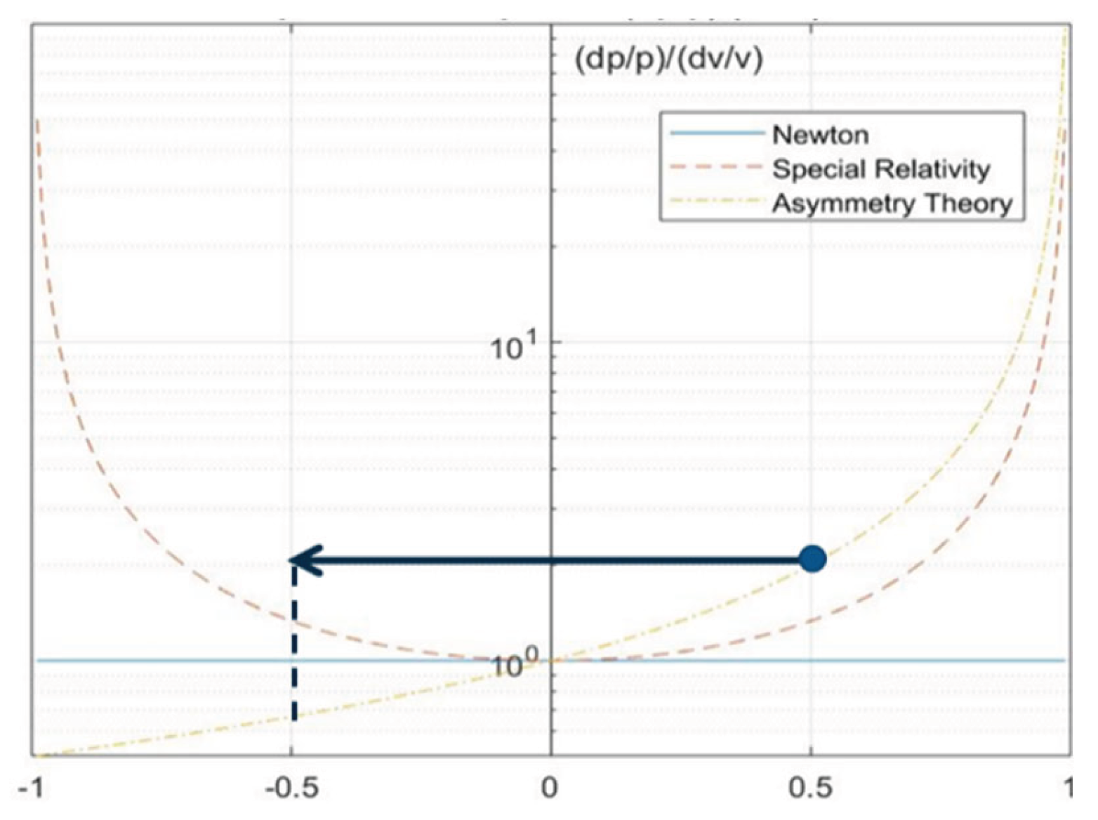
C.: Momentum to speed change ratio anisotropy

Unlike STR, AT Eq. (39) predicts anisotropy in momentum-to-speed-change ratios, which means when a particle is accelerated, it requires more momentum to accelerate further, i.e. “resistance to acceleration”; when decelerated, it requires less momentum, i.e. “inclination to deceleration”. This asymmetry is illustrated in Figure 4.

An experiment was proposed in [23] to test this prediction. Keep a particle at a constant high speed, say 0.5c. Apply a constant momentum to the particle and measure the resulting speed change. Repeat the measurement but change the direction of momentum each time.

AT Eq. (40) predicts an anisotropic ratio $Δ P / Δ v_{o}$ :

Accelerate:

2 m

versus Decelerate:

2 / 3 m

.

STR predicts the ratio is constant for any direction.

The result will confirm if the momentum to speed change is anisotropic or isotropic, distinguishing AT from STR.

IX. Discussion & Future Work

Asymmetry Theory is a mathematically derived, self-consistent framework based purely on one single principle of constant light velocity. AT aligns with all established empirical evidence and reconciles contested results within its unified framework (Table I. AT derivation and evidence).

AT mathematically demonstrates:

Relativistic phenomena do not require abandoning absolute time—they can be derived within classical spacetime from observer-dependent light velocity.
AT reproduces all validated predictions of STR (Table III.) as a special case and extends to non-inertial frames.
Time synchronization and causality are preserved by distinguishing clock variations from real time dilation.
Multiple distinct phenomena (Doppler, redshift, Sagnac, Cherenkov) share common mathematical origin.
Doppler and Sagnac effects are solved directly from an observer-frame formulation of Maxwell’s equations, which eliminates the need for GED approximation.
Sagnac effect formula is directly derived from one-way light speed without assuming rotational frame.

AT makes novel testable predictions distinguished from STR (Table IV.), which will be the future work of empirical validation. A motion-controlled interferometer with first-order sensitivity to two-way light speed deviation is proposed for the confirmative test of AT.

AT does not assume the ether or a universal reference frame. Velocity calculations need selecting a frame at rest with the light origin, which is event specific and doesn’t indicate a universal frame — for example, the ECI and CMB frames may work for different phenomena. Frame selection will be based on empirical tests with some methods presented in [48], which will be future work.

In summary, Asymmetry Theory is mathematically rigorous, self-consistent and empirically testable. If validated by further tests, it will have groundbreaking impacts on foundational physics and promote insights into some fundamental questions in areas like optics, particle physics, cosmology and quantum.

Acknowledgments/Funding

This research is sponsored by the international education foundation.

Data Availability

All data generated or analyzed during this study are included in this published article.

Conflict of Interest

The authors declare no conflicts of interest.

Appendix A

A.: The “twin paradox”

Assume a light source is at rest and an observer moves away from the same position and returns. Each records its time as

t_{s}

and

t_{o}

, with the start times synchronized as

t_{s} = t_{o} = 0

, and the return times as

t_{s} = t_{1}

and

t_{o} = t_{1} ’

, respectively. The elapsed times recorded by each can be represented as

\int_{0}^{t_{1}} d t_{s}

and

\int_{0}^{t_{1}^{'}} d t_{o}

, respectively. Using (19) to substitute

d t_{s}

with

d t_{o}

, we have

\int_{0}^{t_{1}} d t_{s} = \int_{0}^{t_{1}^{'}} \frac{c + v_{o} (t_{o}) \cos (θ_{o})}{c} d t_{o} = \int_{0}^{t_{1}^{'}} d t_{o} + \frac{1}{c} \int_{0}^{t_{1}^{'}} v_{o} (t_{o}) \cos (θ_{o}) d t_{o} = \int_{0}^{t_{1}^{'}} d t_{o} + \frac{1}{c} \oint_{L} \cos (θ_{o}) d s

Where

d s

is the incremental distance over the path

L

. Since L is a closed contour,

\oint_{L} \cos (θ_{o}) d s = 0

. We have:

\int_{0}^{t_{1}} d t_{s} = \int_{0}^{t_{1}^{'}} d t_{o} o r t_{1} = t_{1}^{'}

(52)

B.: Lorentz Force invariance across observer frames

The Lorentz force formula (38) for a particle P is

F = q * (E + v_{o} \times B)

Like the light origin, let

S

be the center of the magnetic field

B

. Hence, we have:

v_{o} = \frac{d (P - S)}{d t}

If we perform the Galilean transformation,

P, S, E, B

become

P^{'}, S^{'}, E^{'}, B^{'}

after transformation. We should have the same Lorentz force after transformation. Hence,

q * (E^{'} + v_{o}^{'} \times B^{'}) = q * (E + v_{o} \times B)

(53)

Since

v_{o}^{'} = \frac{d (P^{'} - S^{'})}{d t^{'}} = \frac{d (P - S)}{d t} = v_{o}

for (53) to hold for any

v_{o}

, we have:

E^{'} = E and B' = B

(54)

In summary, The Lorentz force law in AT is invariant for same observer across different frames and the EM fields don’t change just because of different frame selection.

C.: Observer-Frame Formulation Consistency

For simplicity, assume the light is polarized moving in the x-direction. The Observer-frame formulation of Maxwell equations (31) for an observer

O

in frame

F

becomes:

\frac{\partial^{2}}{\partial x^{2}} E - \frac{1}{{(c - v_{o})}^{2}} \frac{\partial^{2}}{\partial {t_{o}}^{2}} E = 0

(55)

Perform the Galilean transformation from

F

to a new observer frame

F^{'}

. Let

v_{o}, t_{o}, t, E

become

v_{o}^{'}, t_{o}^{'}, t^{'}, E^{'}

after transformation. From (20) we have

\frac{d t_{o} ’}{d t^{'}} = \frac{c}{c - v_{o} ’} a n d \frac{d t_{o}}{d t} = \frac{c}{c - v_{o}}

Since

t^{'} = t

, we have

\frac{d t_{o}}{c - v_{o}} = \frac{d t_{o}'}{c - v_{o}'}

Since

E^{'} = E

from (54), substituting

t_{o}, v_{o}

with

t_{o}^{'}, v_{o} ’

in (55), we have:

\frac{\partial^{2}}{\partial x'^{2}} E^{'} - \frac{1}{{(c - v_{o}')}^{2}} \frac{\partial^{2}}{\partial t_{o}'^{2}} E^{'} = 0

(56)

which keeps the same form of (55).

In summary, the Observer-Frame formulation (31) maintains the same form across different reference frames.

Important Note: This is NOT traditional Galilean covariance, which fails for EM. Here, only the observer’s motion went through the Galilean transformation. Hence, It is “observer-frame consistency”— i.e. different observers of the same EM take the same form of equations, i.e. classical velocity addition.

References

Einstein, On the Electrodynamics of Moving Bodies. Annalen der Physik 1905, 17, 891–921.
Einstein, Does the Inertia of a Body Depend Upon its Energy-Content? Annalen der Physik 1905, 323(13), 639–641.
Einstein, On the Possibility of a New Test of the Relativity Principle. Annalen der Physik 1907, 328(6), 197–198.
Einstein, Generalized theory of relativity, the anthology ‘The Principle of Relativity’, 94, University of Calcutta; 1920.
Maxwell, A Dynamical Theory of the Electromagnetic Field. Philos. Trans. R. Soc. Lond 1865, 155, 459–512.
Lorentz, Electromagnetic phenomena in a system moving with any velocity smaller than that of light. Proc. R. Neth. Acad. Arts Sci. 1904, 6, 809–831.
Michelson; Morley, E. On the Relative Motion of the Earth and the Luminiferous Ether. Am. J. Sci. 1887, 34(203), 333–345. [Google Scholar] [CrossRef]
Brecher, K. Phys. Rev. Lett. 1977, 39, 1051. [CrossRef]
Ritz, W. Recherches Critiques sur les Theories Electrodynamiques de Cl. Maxwell et de H.-A. Lorentz. Archives des Sciences physiques et naturelles 1908, 36, 209. [Google Scholar]
Fox, Evidence Against Emission Theories. Am. J. Phys. 1965, 33(1), 1–17.
Alvaeger. Phys. Lett. 1964, 12, 260. [CrossRef]
Babcock. J. O. S. A. 1964, 54, 147. [CrossRef]
Champeney, D.C. Absence of Doppler shift for gamma ray source and detector on same circular orbit. Proc. Phys. Soc. 1961, 77, 350. [Google Scholar] [CrossRef]
W., H. THIM, Absence of the relativistic transverse Doppler shift at microwave frequencies. IEEE Trans. Instr. Measur 2003, 52, 1660–1664. [Google Scholar] [CrossRef]
Sagnac, C. Acad. Sci. Paris 1913, 157, 708.
Wang. Physics Letters A 2006, 312(1–2), 7–10. [CrossRef]
Langevin, P. Sur la théorie de la relativité et l’expérience de M. Sagnac. Comptes Rendus 1921, 173, 831–834. [Google Scholar]
Barnett, S.J. On Electromagnetic Induction and Relative Motion. Phys. Rev. 1912, 35, 323. [Google Scholar] [CrossRef]
Sher, The Relativistic Doppler Effect. J. R. Astron. Soc. Can. 1968, 62, 105–111.
Giordano, N. College Physics: Reasoning and Relationships. In Cengage Learning; 2009; pp. 421–424. [Google Scholar]
Koupelis. Quest of the Universe; Jones & Bartlett Publishers, 2007; p. 557. [Google Scholar]
Lorentz, Versuch einer Theorie der electrischen und optischen Erscheinungen in bewegten Körpern; E.J. Brill: Leiden, 1895.
Chen, Q. Design of Experiments for Light Speed Invariance to Moving Observers. 2021. [Google Scholar] [CrossRef] [PubMed]
Chen, Q. Time-varying Doppler Effect formula and its application. 2021. [Google Scholar] [CrossRef]
Chen, Q. Asymmetry Theory mathematically derived from the principle of constant light speed. 2021. [Google Scholar] [CrossRef]
Nelson, R.A. Experimental Comparison of Time Synchronization Techniques by Means of Light Signals and Clock Transport on the Rotating Earth. Proc. 24th Annual PTTI Systems and Applications Meeting, 1993; pp. 87–104. [Google Scholar]
Gezari, D.Y. Lunar laser ranging test of the invariance of c. arXiv 2009. [Google Scholar]
Chou. Optical clocks and Relativity. Science 2010, 329(5999), 1630–1633. [Google Scholar] [CrossRef]
Hafele. Around-the-World Atomic Clocks: Observed Relativistic Time Gains. Science 1972, 177(4044), 168–170. [Google Scholar] [PubMed]
Ives, E. An experimental study of the rate of a moving atomic clock. J. O. S. A. 1938, 28(7), 215. [Google Scholar] [CrossRef]
Rossi. Variation of the Rate of Decay of Mesotrons with Momentum. Physical Review 1941, 59(3), 223–228. [Google Scholar]
Kaufmann, W. Die magnetische und elektrische Ablenkbarkeit der Bequerelstrahlen und die scheinbare Masse der Elektronen. Göttinger Nachrichten 1901, (2), 143–168. [Google Scholar]
Oliphant, M.L.E. “The Transformation of Lithium by Protons and by Ions of the Heavy Isotope of Hydrogen”. Proc. R. Soc. 1933, 141(845), 722–733. [Google Scholar]
Cherenkov, P. A. Visible emission of clean liquids by action of γ radiation. Doklady Akademii Nauk SSSR 1934, 2, 451. [Google Scholar]
Chen, Q. A unified formula for Time-Varying Doppler effect, Cosmological red-shift and Cherenkov radiation. Optica 2024. [Google Scholar] [CrossRef]
Reinhardt, S. Test of relativistic time dilation with fast optical atomic clocks at different velocities. Nature Physics 2007, 3(12), 861–864. [Google Scholar] [CrossRef]
Doppler. Beiträge zur fixsternenkunde; G. Haase Söhne: Prague, 1846; p. 69. [Google Scholar]
Bélopolsky. On an Apparatus for the Laboratory Demonstration of the Doppler-Fizeau Principle. ApJ. 13 1901, 15. [Google Scholar] [CrossRef]
P. Marmet, The GPS and the Constant Velocity of Light. Acta Scientiarum 2000, 22, 1269.
Chen, Q. Revisiting Maxwell’s Equations for Observers. 2024. [Google Scholar] [CrossRef]
de Broglie. Recherches sur la théorie des quanta. Thèse de doctorat soutenue, Paris, 1924. [Google Scholar]
Zhang, Y.Z. Special Relativity and Its Experimental Foundation; World Scientific, 1997; Vol. 4. [Google Scholar]
Joos. Annalen der Physik 1930, 399(4), 385–407. [CrossRef]
Brillet; Hall, J. L. Physical Review Letters 1979, 42, 549. [CrossRef]
Herrmann, S. Physical Review D 2009, 80, 105011. [CrossRef]
Chen, Q. Novel Interferometer with First-Order Sensitivity for Detecting Two-Way Light Speed Deviations. Optica 2025. [Google Scholar] [CrossRef]
Penzias, A.A.; Wilson, R.W. The Astrophysical Journal 1965, 142(1), 419–421. [CrossRef]
Chen, Q. U.S. Patent No. US, 2024.

Figure 1. Light emission Timing, Velocities and Key angles.

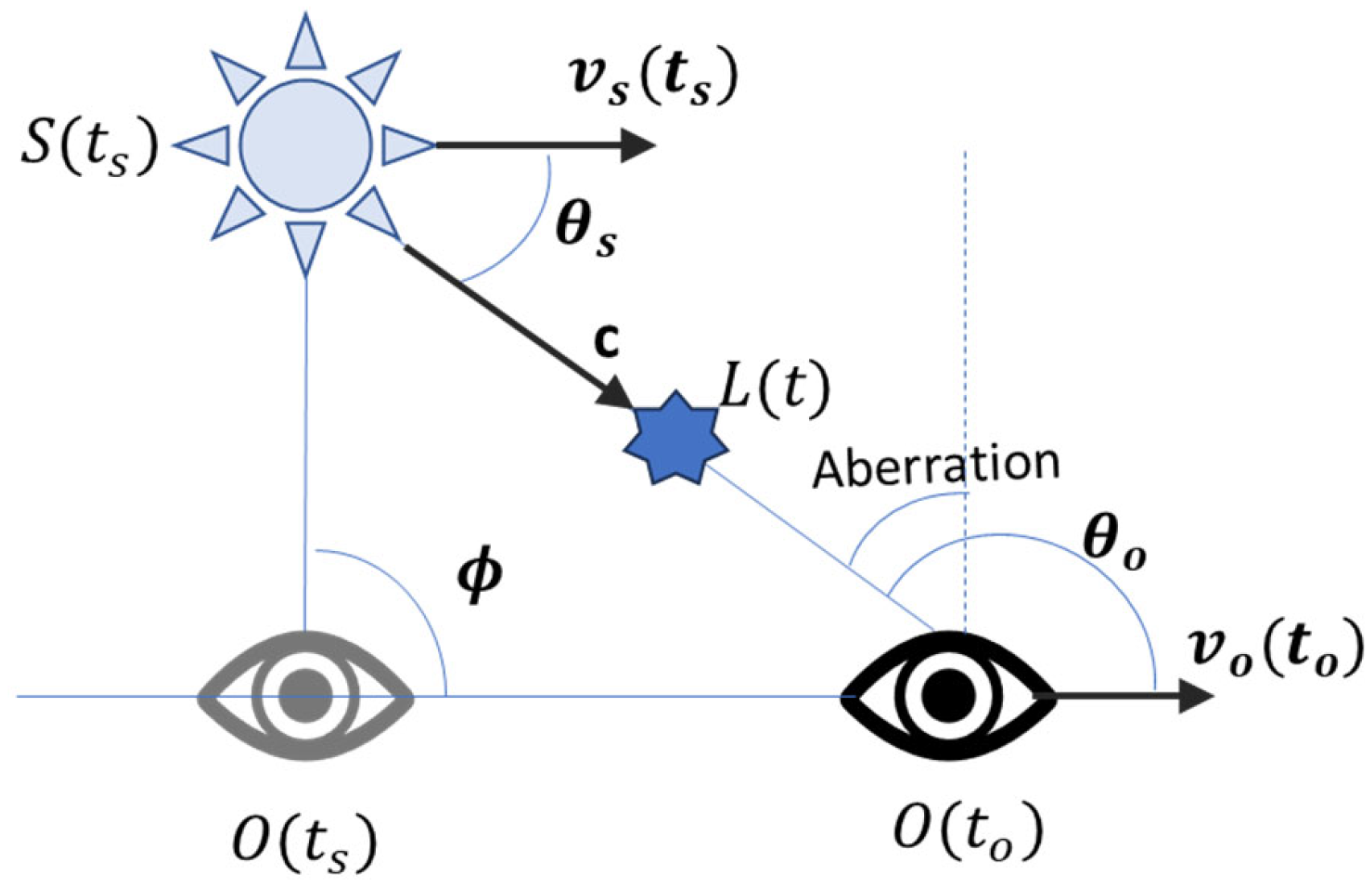
Figure 2. Light cones in Asymmetry Theory.

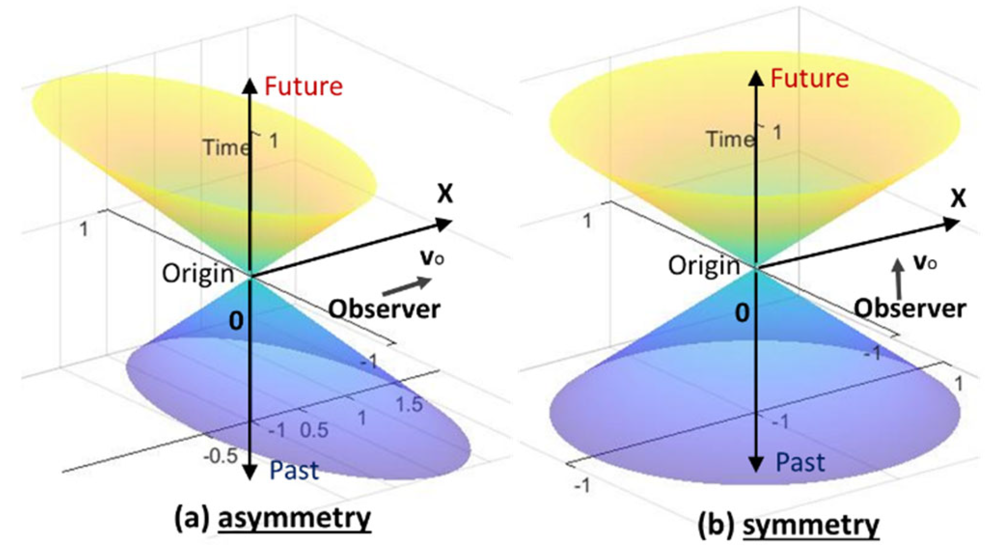
Figure 3. Interferometer detecting light speed deviation [46].

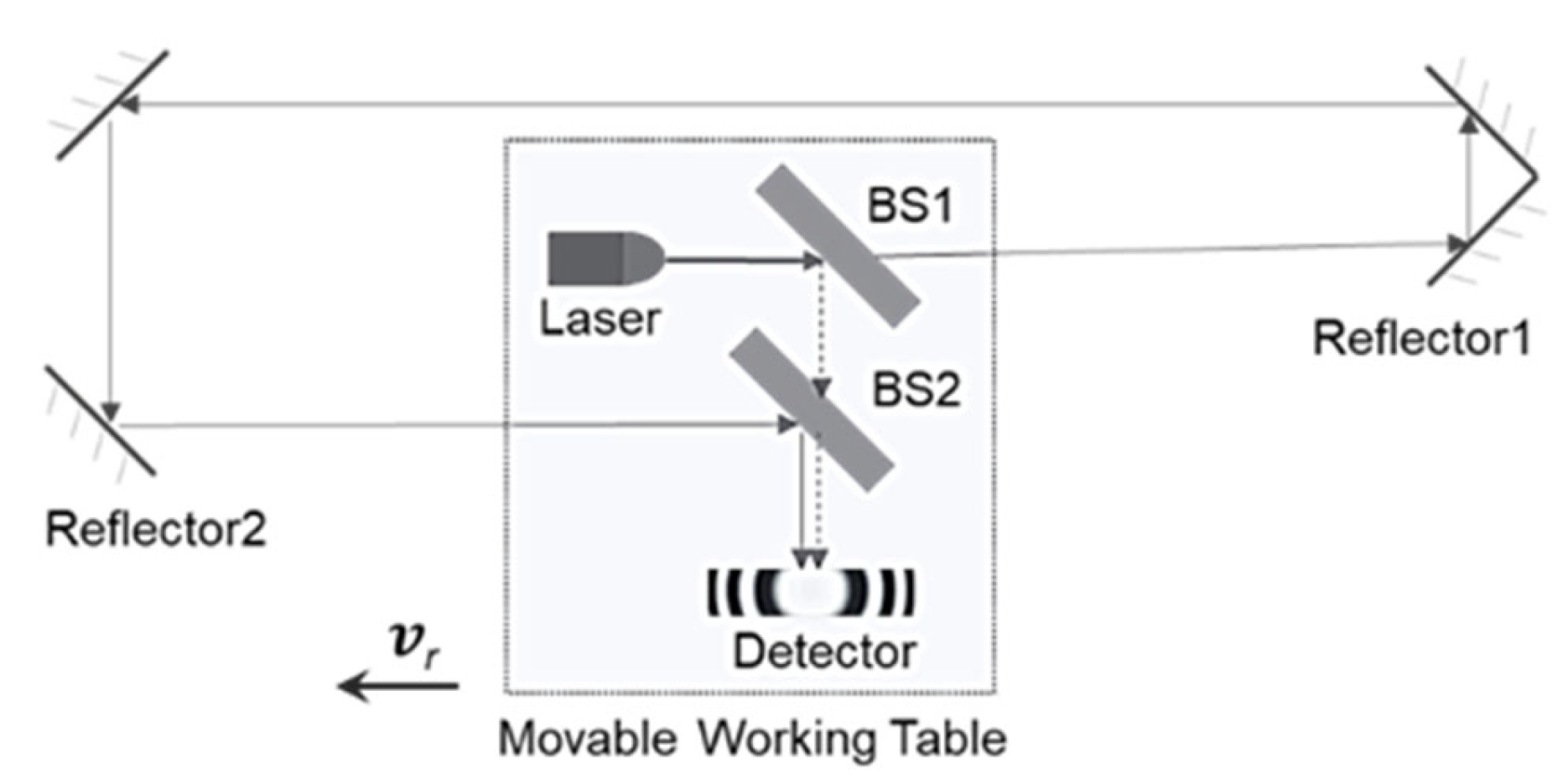
Figure 4. Asymmetry of momentum to acceleration ratio [23].

Disclaimer/Publisher’s Note: The statements, opinions and data contained in all publications are solely those of the individual author(s) and contributor(s) and not of MDPI and/or the editor(s). MDPI and/or the editor(s) disclaim responsibility for any injury to people or property resulting from any ideas, methods, instructions or products referred to in the content.

© 2026 by the authors. Licensee MDPI, Basel, Switzerland. This article is an open access article distributed under the terms and conditions of the Creative Commons Attribution (CC BY) license (http://creativecommons.org/licenses/by/4.0/).

Copyright: This open access article is published under a Creative Commons CC BY 4.0 license, which permit the free download, distribution, and reuse, provided that the author and preprint are cited in any reuse.

Asymmetry Theory: A Unified Mathematical Framework for Classical and Relativistic Phenomena from Principle of Light-Speed Constancy

Abstract

Keywords:

Subject:

I. Introduction

II. Light Velocity

III. Empirical Evidence

IV. Unification of Doppler Effect

VI. Electrodynamics

VII. Relationship with STR

VIII. Novel Testable Predictions

IX. Discussion & Future Work

Acknowledgments/Funding

Data Availability

Conflict of Interest

Appendix A

References

MDPI Initiatives

Important Links

Subscribe