
Submitted:
17 January 2026
Posted:
20 January 2026
You are already at the latest version
Abstract
In this work we formulate a geometry-independent holographic principle within the Holographic Bit-Mode Balance (HBMB) framework, interpreting the Bekenstein-Hawking entropy as a physical resolution bound. Our starting point is that for a horizon/screen of radius R, the bit capacity S(R)=A(R)/(4l_P^2) is not merely an information-theoretic upper limit, but directly constrains the maximal number of independent bulk eigenmodes that can be represented. Accordingly, wavefunction-like bulk field data admit a finite eigenmode synthesis: screen-encoded mode amplitudes (coefficients) reconstruct a complex field psi in a geometry-dependent eigenbasis within a chosen local domain (patch) associated with the screen. The main claim is that this "holographic Nyquist" logic is not AdS-specific. In local cosmological (dS) patches, flat-space domains, and AdS regions, the same capacity argument yields a physical cutoff, lmax(R) approx sqrt{S(R)}-1, which controls reconstruction accuracy. We provide a unified toy-model protocol for numerical reconstruction of target fields and show that the reconstruction error decreases systematically as the Bekenstein-cutoff bound is approached. Finally, we discuss the "nested horizons" picture in which local horizons (black holes, local cosmological horizons, microscopic effective horizons) are interpreted as overlapping subcodes of a universe-scale master-horizon code, rather than as mutually independent entropy budgets. We also note that an "edge-physics" intuition is compatible with the code-subspace viewpoint: screen boundary data can be regarded as operational coordinates of an edge-mode algebra, rather than a purely mathematical choice of basis.
Keywords:
holographic principle
; Holographic Bit-Mode Balance (HBMB)
; Bekenstein-Hawking entropy
; horizon entropy
; information bound
; mode cutoff
; eigenmode reconstruction
; bulk reconstruction
; HKLL smearing
; AdS/CFT
; de Sitter space
; anti-de Sitter space
; flat spacetime
; spherical harmonics
; spectral truncation
; Nyquist sampling
; resolution bound
; holographic screen
; nested horizons
; quantum error correction
; code subspace
; edge modes
; entanglement wedge
; FFT
1. Introduction
1.1. Motivation: Local Holography Beyond AdS
One of the deepest implications of the holographic principle is that in gravitational systems the number of independent physical degrees of freedom scales with the boundary area rather than the bulk volume. The Bekenstein–Hawking entropy makes this statement particularly concrete: the area of a horizon determines how much information can be encoded “on the boundary” [1,2]. The AdS/CFT correspondence provides the most explicit and powerful realization of this idea [5,6,7], where a -dimensional AdS bulk gravitational theory is equivalent to a d-dimensional boundary CFT. In this setting, bulk reconstruction from boundary data can be discussed via concrete procedures [9]. In the modern picture, quantum entanglement acquires geometric meaning (Ryu–Takayanagi and its covariant extensions) [10,11], and the holographic code-subspace / quantum error correction (QEC) viewpoint has become central [12,13].
However, two foundational questions remain pressing, especially if holography is to be understood beyond global AdS boundaries. First: how does boundary-stored information become a concrete, local 3D “bulk reality,” such as a field configuration or a wavefunction? Second: in what sense can holographic reconstruction be generalized to local horizons (e.g., de Sitter static patches, black hole horizons, or microscopic effective horizons) where the standard AdS/CFT boundary structure is not available?
In this paper we explore the viewpoint that the key ingredient for local holography may not be the explicit knowledge of a special boundary theory (a CFT), but rather the physical capacity constraint set by the horizon entropy itself. The central claim is that the Bekenstein–Hawking entropy is not only an “information maximum,” but also a resolution bound for what can be represented and reconstructed in the bulk: it determines how many independent eigenmodes can be encoded without loss for a given local horizon.
1.2. HBMB Background: Bit–Mode Balance and Fixed-Point Intuition
The Holographic Bit–Mode Balance (HBMB) concept asserts that a horizon’s bit capacity and the number of independent bulk modes are tied by a balance relation. Heuristically, if one attempts to maintain more independent modal degrees of freedom in the bulk than the horizon-projected code capacity permits, the description cannot remain stable. In this sense HBMB can be viewed as a Nyquist-like principle in which the horizon plays the role of sampling: the number of available bits fixes the maximal reconstructible spectral content [15,16]. The goal of the present work is to turn this “counting” statement (comparing bit and mode counts) into an explicit reconstruction principle: how a bulk wavefunction arises from the horizon-encoded mode amplitudes.
1.3. Contributions
The paper provides three main contributions:
- 1.
- Generalized local holographic principle (HBMB eigen-reconstruction): we formulate that bulk wavefunctions can be reconstructed by a finite eigenmode synthesis whose maximal angular order is fixed by the Bekenstein–Hawking entropy of the relevant horizon.
- 2.
- Non-AdS-specific cutoff logic: we show that the reconstruction principle can be implemented in flat-space domains, de Sitter static patches, and AdS regions; the distinction appears only through the geometry-dependent eigenbasis.
- 3.
- Nested horizons as overlapping codes: we discuss the picture in which local horizons are overlapping subcodes of a universe-scale master-horizon code, avoiding the naive conclusion that local entropies should simply be added.
1.4. Paper Outline
Section 2 reviews related results (bulk reconstruction in AdS/CFT, entanglement-wedge and code-subspace/QEC intuition, and classical tools from spectral geometry) and states precisely what is novel in the present approach. Sections 3–5 introduce the definitions, the HBMB-linked Bekenstein cutoff, and the general form of local eigenmode reconstruction. Sections 6 and 7 present numerical toy-model demonstrations of reconstruction across different geometries. Section 8 discusses the nested-horizons picture, while Sections 9 and 10 summarize connections, scope, limitations, and potentially testable consequences.
2. Related Work and Novelty
In this section we place the present work within the holography literature and state precisely what is new. A key point is clarified upfront: eigenfunction decompositions and Fourier dualities are standard tools in quantum mechanics, so our claim is not that the underlying mathematics is new. Rather, the novelty is that a horizon-entropy-derived physical capacity constraint (HBMB) fixes the reconstructible spectral content in a natural, non–AdS-specific way.
2.1. Holography and Bulk Reconstruction in AdS/CFT
The best-developed realization of the holographic principle is the AdS/CFT correspondence [3,4,5,6,7], in which a -dimensional AdS bulk gravitational theory is equivalent to a d-dimensional boundary conformal field theory (CFT). Within this framework, the “bulk reconstruction” problem—i.e., how to represent bulk operators in terms of boundary degrees of freedom—appears in several closely related forms.
Two foundational formulations are the GKPW dictionary (Gubser–Klebanov–Polyakov–Witten) [6,7], where boundary correlators are generated by functional differentiation with respect to boundary sources, and the BDHM dictionary (Banks–Douglas–Horowitz–Martinec) [8], where boundary operators are associated with suitably rescaled boundary limits of bulk fields. In AdS these dictionaries can be reconciled, but the detailed matching can involve scheme- and normalization-dependent factors, especially for composite operators and their renormalization [14].
A concrete operator-level construction is provided by HKLL (Hamilton–Kabat–Lifschytz–Lowe) [9], which builds approximate local bulk operators as smeared integrals of boundary operators under appropriate assumptions. Modern developments emphasize that reconstruction is not merely an operator identity, but has an information-theoretic and code-theoretic structure: in the holographic code-subspace / quantum error correction (QEC) viewpoint, bulk information is encoded redundantly and in an overlapping manner across boundary subsystems [12,13]. This is closely tied to the notion of the entanglement wedge, which specifies the bulk region reconstructible from a given boundary region. In parallel, entanglement acquires geometric meaning via the Ryu–Takayanagi relation and its covariant generalizations [10,11], where boundary entanglement entropies are computed by areas of extremal bulk surfaces.
2.2. Operator Dictionaries and the Wavefunction Formalism: What Changes in dS?
For the purposes of the present work it is important that the “equivalence” of holographic dictionaries is strongly AdS-specific. A detailed analysis by Harlow and Stanford shows that while in AdS the GKPW- and BDHM-type dictionaries can be made equivalent with suitable definitions, the situation in de Sitter space is substantially more subtle: the late-time boundary is spacelike, and the usual “source–response” logic and boundary-condition fixing do not carry over straightforwardly [14]. In this context the wavefunction formulation becomes the natural language: physical probabilities are obtained via the Born rule from , and the cleanest analytic continuations between AdS and dS are often expressed at the level of rather than directly at the level of expectation values [14].
This observation matters here for two reasons. First, it reinforces the broader message that holographic reasoning should not be confined to AdS: in dS the wavefunction can be the primary object. Second, it supports the central theme of the present paper: a “horizon data → bulk wavefunction” reconstruction principle is not an arbitrary mathematical game, but a perspective aligned with the fact that wavefunction-level holography is structurally preferred in the de Sitter setting [14].
2.3. Not Just Fourier: What Is New in the HBMB Approach?
In quantum mechanics, decomposing a wavefunction into modes (Fourier series, Fourier transforms, or more generally spectral decompositions) is standard. Position- and momentum-space wavefunctions are Fourier dual, and depending on the domain one naturally uses Fourier series (periodic case) or Fourier transforms (non-compact line). Therefore, the statement that “a wavefunction is a sum of modes” is not by itself a new physical claim.
The novelty of the present work is that the truncation of the mode expansion (the cutoff) is not introduced as a numerical convenience, but is derived from a physical capacity bound. In the HBMB viewpoint, the Bekenstein–Hawking entropy associated with a horizon of radius R [1,2] fixes the maximal number of independent boundary bits that can be encoded. We identify this bit budget with the maximal number of independent bulk mode coefficients in an appropriate geometry-dependent eigenbasis. For a spherical angular decomposition, the number of independent angular modes up to is
so HBMB naturally yields a “Nyquist-like” capacity condition [15,16]: the horizon bit capacity fixes the maximal reconstructible spectral content of bulk fields.
We emphasize that this “holographic Nyquist principle” does not mean that the literal factor of the Nyquist theorem appears in geometry. The similarity is structural: lossless reconstruction requires that the available coding capacity be at least as large as the number of degrees of freedom to be reconstructed. If one attempts reconstruction for a fixed horizon while targeting a state whose effective “bandwidth” exceeds that horizon’s bit budget, reconstruction becomes non-unique and exhibits cutoff-induced artifacts. In the HBMB interpretation this should not necessarily be read as fundamental information loss; rather, it diagnoses an inconsistent horizon assumption for the chosen state class. In a consistent physical evolution, such a mismatch may trigger an effective code/horizon reconfiguration (e.g., increased effective R or patch reallocation), so the “cutoff error” in toy models is best understood primarily as a diagnostic and a characteristic signature.
2.4. Positioning of the Present Work
In summary, the AdS/CFT reconstruction literature demonstrates that bulk–boundary duality can be formulated at the operator level and at an information-theoretic (QEC) level [9,12,13], and that entanglement plays a central geometric role [10,11]. Work on dS holography and on dictionary subtleties highlights that wavefunction-based formulations are not a minor technical detail, but often the most natural language in de Sitter contexts [14].
Against this background, HBMB emphasizes a different organizing principle: we do not construct a boundary-CFT operator dictionary, but formulate a local-horizon reconstruction rule whose cutoff is fixed by horizon entropy. The central novelty is that the cutoff is not chosen by hand, but derived from the Bekenstein–Hawking entropy, and is then demonstrated numerically via a unified toy-model protocol across different geometries (flat space, dS, AdS). This viewpoint provides a natural bridge between standard spectral quantum mechanics and the holographic code-subspace perspective, while remaining explicitly meaningful for local horizons.
3. Basic Concepts and a Formal Statement of the HBMB Reconstruction Principle
In this section we introduce the minimal set of definitions and notation needed to state the “horizon bits → bulk wavefunction” reconstruction principle precisely. Our goal is not to build a complete quantum-gravitational formalism, but to fix a geometry-dependent yet conceptually general procedure that later toy models and numerical demonstrations can rely on unambiguously.
3.1. What Do We Call a Horizon in This Paper?
We consider an observer-associated local horizon that acts as an effective coding surface for that observer. Throughout the paper we use the term “horizon” in a deliberately broad sense: not only a global event horizon, but any boundary surface that naturally separates an “inside” region for the observer and admits an information-capacity / reconstructability bound.
We denote by R the characteristic radius of the horizon. In a chosen coordinate system, the reconstruction domain is taken to be the interior region:
where r is a radial coordinate.
Concretely, we include:
- 1.
- Cosmological horizon (dS static patch): in de Sitter space, the cosmological horizon of the static patch, naturally associated with Gibbons–Hawking temperature and entropy [17].
- 2.
- 3.
- Rindler horizon (remark): the kinematic horizon for uniformly accelerated observers; included only to emphasize that “horizon as a code surface” is not exclusive to gravitational collapse. The associated thermality is the Unruh effect [18].
- 4.
- Micro-horizon (HBMB-language definition): in the HBMB viewpoint, a micro-horizon is any sufficiently small effective boundary surface to which a Bekenstein–Hawking-type capacity bound can be assigned (at least heuristically), thereby defining a local spectral cutoff. Here the term is used as a toy-model concept: it encodes the statement that HBMB logic can be formulated locally (including particle-scale contexts) at the level of principle.
3.2. Horizon as a Local Code Surface: Entropy and Bit Capacity
Let denote the horizon area and the Planck length. The Bekenstein–Hawking entropy is
In this work, is used as a dimensionless capacity scale in two complementary ways [1,2]:
- 1.
- Bit capacity: sets the order of magnitude of the maximal number of independent information units (bits/qubits) that can be encoded on the horizon.
- 2.
- Resolution bound: also acts as a resolution limit: a description based on a fixed horizon cannot reliably represent arbitrarily fine bulk structure, because that would require more independent coding degrees of freedom than are available on the horizon.
Hence, a local horizon defines a finite-dimensional code space: the “bandwidth” of a horizon-based description is bounded by .
3.3. What Is the Reconstruction Domain?
We restrict reconstruction to the observer’s statically meaningful interior region. In toy models this is imposed explicitly as
Specific coordinate choices (e.g., dS static coordinates, a spherical domain in flat space, or a cut-off region in AdS) and normalizations are part of the numerical implementation and will be fixed in later sections.
3.4. What Do We Mean by “Boundary Data”?
In this paper “boundary data” does not mean abstract boundary sources in the GKPW sense. Instead, it refers concretely to the set of mode amplitudes associated with the horizon. For a spherical angular decomposition, this is naturally the set of coefficients , where ℓ and m are spherical-harmonic indices.
In toy models, boundary data may appear in two equivalent forms:
- 1.
- Coefficient form: boundary data is directly given as the amplitudes (or, including radial indices, ), which weight the bulk eigenmodes.
- 2.
- Sampled form: boundary data is specified as discretized samples on the boundary, e.g., values on the surface, from which can be estimated numerically (e.g., via a discrete spherical-harmonic transform or least-squares fitting).
3.5. Bulk Eigenmodes: The Minimum of Spectral Geometry
On the bulk side, consider a wavefunction or field configuration , where x denotes coordinates in the interior domain. In spherical coordinates one may take . The reconstruction idea is that can be expanded in eigenfunctions of a geometry-adapted differential operator.
Formally:
- choose a differential operator L natural to the background geometry (typically the Laplace–Beltrami operator for scalar fields, or a Dirac-type operator for spinors in a simplified toy-model setting),
- solve the eigenvalue problem on the domain with chosen boundary conditions:where is the n-th eigenmode (eigenfunction), its eigenvalue, and n may be a compound index (e.g., ).
Then admits the formal expansion
Compared to a standard Fourier series, the basis here consists of geometry- and boundary-condition-adapted eigenfunctions.
3.6. What Do the Mode Coefficients Mean?
The mode coefficients are the amplitudes associated with the basis modes: they quantify how strongly the state contains each eigenmode .
If the modes are normalized to form an orthonormal basis on with respect to a suitable inner product, the coefficients are obtained by projection:
where is the chosen inner product (for a scalar field, typically a volume integral with the appropriate geometric measure).
In the quantum-mechanical interpretation, if represent eigenstates of an observable, then is proportional to the probability of obtaining the corresponding eigenvalue upon measurement.
For spherical angular decompositions, the notation becomes and, for example, the angular dependence can be written as
where are spherical harmonics.
3.7. HBMB as a Physical Cutoff: A “Bandlimit” for the Mode Space
The expansion above is mathematically infinite. The HBMB claim is that a horizon’s bit capacity implies a finite number of physically representable modes, and that this truncation (cutoff) should be fixed by rather than chosen ad hoc.
For a spherical angular decomposition, the number of independent angular modes up to is
In toy models we impose the HBMB capacity condition
where is an correction factor accounting for field-dependent redundancies (spin/polarization, complex amplitudes, gauge degrees of freedom). In the simplest demonstrations we start with .
3.8. Local Holographic Eigenmode Reconstruction (HBMB Principle)
In this subsection we state the central claim of the paper: how horizon-stored spectral information becomes a bulk wavefunction (or field configuration) defined on an interior region. The presentation is intentionally toy-level but mathematically explicit: we formulate a reconstruction principle that does not rely on an asymptotic AdS boundary or a specific CFT, but only on (i) an observer-associated local horizon and (ii) the eigenmodes adapted to the background geometry.
3.8.1. Principle Statement
Statement (HBMB reconstruction principle): Let an observer-associated local horizon be characterized by a radius R, and consider the interior domain . Assume that on the local horizon we have a boundary data set that can be represented as a collection of mode amplitudes (coefficients) in an appropriate basis. Then the bulk wavefunction / field configuration in the interior domain can be expanded in a geometry-adapted eigenmode basis, and can be reconstructed by a cutoff (truncated) eigenmode synthesis up to the spectral cutoff fixed by the local-horizon bit capacity.
In short: local-horizon data → mode coefficients → cutoff eigenmode synthesis → bulk reconstruction.
3.8.2. General Spectral Form (Eigenmode Synthesis)
In the simplest (S2-symmetric) toy setting, we write the bulk field as
where are spherical harmonics (angular basis), are radial basis functions (depending on the background geometry and boundary conditions), and are mode coefficients (amplitudes) representing the spectral form of the boundary data.
In toy models it is often sufficient to demonstrate purely angular reconstruction. Numerically, to avoid coordinate singular behavior at the horizon one may represent the local horizon by a regulated surface with . In that case one can fix r and treat the radial factor as constant (e.g., ), reducing (11) to the standard spherical-harmonic synthesis on .
The “inverse FFT” analogy is structural: one performs synthesis in a chosen basis, but the basis is provided by the spectral geometry of the spacetime (eigenfunctions) rather than plane-wave sines/cosines.
3.8.3. What Do We Mean by “Boundary Data” in HBMB Language?
In this paper, “boundary data” does not necessarily mean GKPW-type boundary sources in the asymptotic AdS sense. Instead it refers concretely to either
- sampled field values on the local-horizon surface, , or
- their spectral representation, i.e., the set of mode coefficients .
These two descriptions are equivalent: given samples one can compute by projection (integrals or numerical quadrature), and given one can reconstruct the angular dependence via spherical-harmonic synthesis.
In HBMB language, are the spectral coordinates of the horizon “code”: the accessible amplitude data associated with independent degrees of freedom on the local horizon.
3.8.4. Mode Coefficients: Meaning and Estimation
The mode coefficients are amplitudes in the geometric basis. If the spherical harmonics are orthonormal, the coefficients are obtained by projection:
where .
Interpretation: in quantum-mechanical language are not merely “mathematical coefficients”: they quantify the amplitude of the state in the corresponding eigenmode. The HBMB viewpoint is that these amplitudes are naturally associated with the local horizon, i.e., they appear as encoded boundary data accessible to the observer.
3.8.5. The Radial Part and the Role of Geometry
The radial basis functions arise from the eigenfunctions of an operator adapted to the chosen background geometry and field type (e.g., Laplace–Beltrami for a scalar toy model; later, Dirac-type operators for spinor toy models). At toy level, we only need the following:
- the angular basis is natural for any -like local horizon,
- the radial part depends on the background (flat / dS / AdS / Kerr–AdS) and on boundary conditions.
Hence, differences between geometries will primarily manifest through the shape of and the associated spectral structure, while the “local horizon → bulk” logic remains unchanged.
3.8.6. Including the Cutoff: HBMB as a Spectral Bandlimit
HBMB asserts that reconstruction does not involve infinitely many modes: the local-horizon information capacity induces a natural spectral cutoff. In the spherical-harmonic toy setting this reads
The reconstructed field is therefore given by a cutoff (truncated) mode synthesis:
The explicit form of is fixed earlier from the Bekenstein–Hawking capacity and the HBMB postulate.
Physical meaning: the cutoff expresses a maximal “resolution” available to a description tied to a given local horizon: sufficiently high-ℓ modes cannot be stably encoded given finite boundary capacity. In toy models this appears as a reconstruction error and, for sharply localized targets, as Gibbs/ringing-type artifacts.
3.8.7. Brief Relation to AdS/CFT Reconstruction (Positioning)
The principle above is conceptually related to standard holographic reconstruction (bulk operators from boundary data), but it is not identical. In AdS/CFT, known constructions such as HKLL show that under suitable conditions local bulk information can be recovered from boundary CFT data [9]. In a similar spirit, the operator-dictionary and wavefunction viewpoint highlights nontrivial mappings between boundary data and bulk state descriptions [14].
However, the present work does not assume a full CFT or an asymptotic AdS boundary. Here the “boundary” is the observer’s local horizon (in dS, for black holes, or as a toy “micro-horizon”), and the reconstruction is formulated directly in terms of eigenmode synthesis with a capacity-fixed cutoff. The comparison is natural because both viewpoints are spectral/kernel-based, but the geometric and physical starting points differ.
3.8.8. Bridge to the Toy Models
In the following toy-model sections we make the above principle concrete:
This connects “counting” (capacity, mode count, cutoff) to “physics” (wavefunction reconstruction, convergence, error scaling) within a single testable pipeline.
3.9. Boundary Conditions and a “Holographic Residual”: Why It Matters
Modes and coefficients depend not only on geometry but also on boundary conditions. Changing the boundary condition (e.g., Dirichlet ↔ Neumann) changes the spectrum and the mode structure. This is important because one may later define a Casimir-like spectral difference: same geometry, two boundary conditions → two spectra; their difference can define a residual quantity [19]. In the present work we treat this cautiously and only note that boundary conditions are an integral part of reconstruction and must be controlled explicitly in toy models.
3.10. A Brief Scope Remark on Gauge/Dressing
In the presence of gravity and gauge fields, defining local bulk operators and gauge-invariant (dressed) operators is subtle. The present work does not attempt to resolve this problem. Here we treat reconstruction at the level of spectral geometry and toy models; the gauge/dressing issue is included as a scope remark, and we do not claim that the toy models by themselves implement a fully gauge-invariant bulk reconstruction [9].
3.11. A Preview Remark on Measurement and a “Capacity Threshold”
Although our focus is reconstruction, it is worth previewing an interpretational connection: measurement increases the number of effective mode couplings between a system and its environment (apparatus). In an HBMB picture, this can push the effective mode count toward the local code capacity and may induce a “code reconfiguration” above a threshold, which can be interpreted as stabilization of a classical measurement outcome. We only touch this briefly in the present paper.
4. Toy Protocol and Error Metrics
This section fixes a single, geometry-agnostic numerical protocol that turns the HBMB idea from “counting” (capacity + cutoff) into a concrete, testable reconstruction procedure. Later sections (flat / dS / AdS / Kerr–AdS) will only change geometry-specific ingredients (e.g., the choice of R, the radial basis, and boundary conditions), while the pipeline and error metrics remain the same.
4.1. A Unified Reconstruction Pipeline
Let R denote the radius of the observer-associated local horizon.1 We denote the target configuration by and the reconstructed approximation by .
The toy protocol consists of:
- 1.
- Choose a target: specify (angular toy or bulk toy).
- 2.
- Capacity and cutoff: determine and infer .
- 3.
- Estimate mode coefficients: compute via projection (quadrature) or fitting.
- 4.
- Reconstruct: build from modes with .
- 5.
- Measure errors: evaluate , , and optional spectral diagnostics.
- 6.
- Scaling: study the error as a function of up to the capacity-implied cutoff.
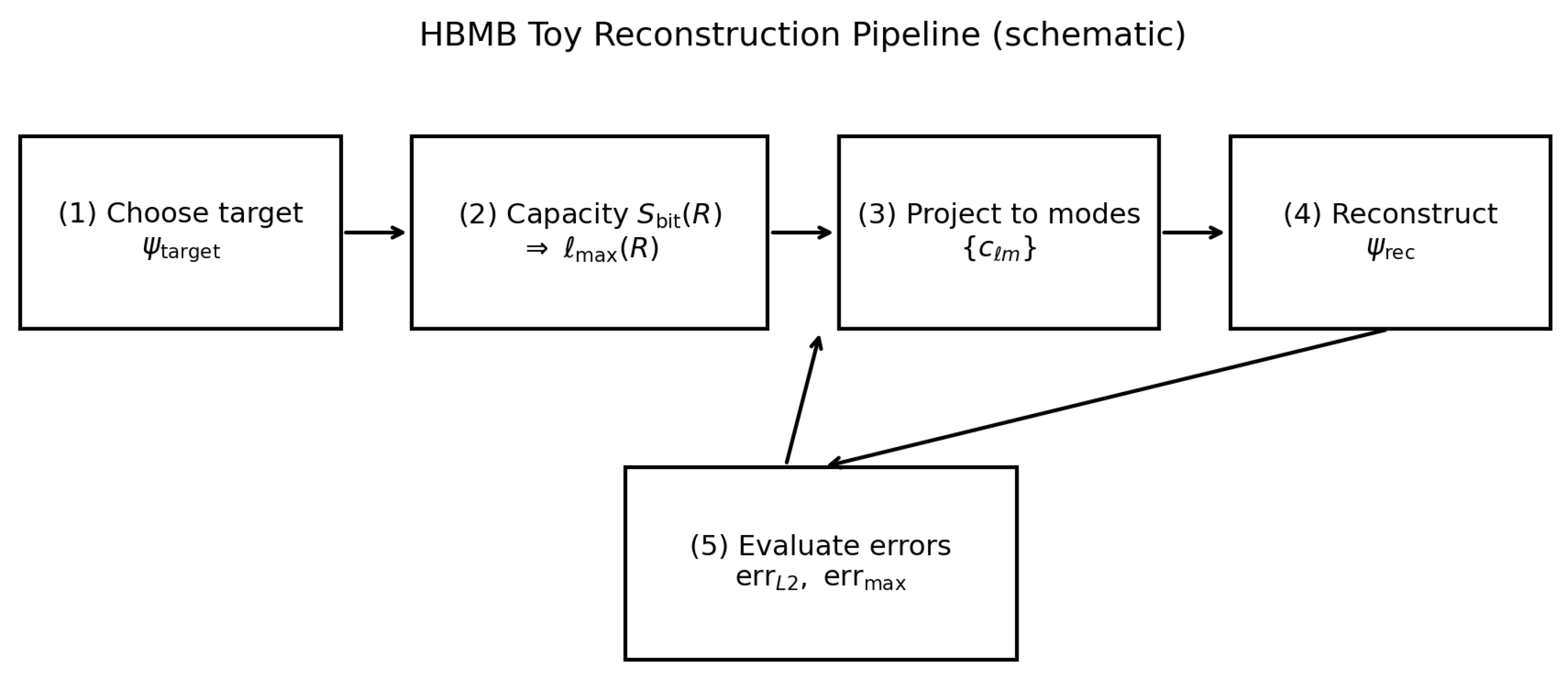
Figure 1.
Schematic overview of the HBMB toy reconstruction pipeline: target field → capacity-implied cutoff → projection to → eigenmode synthesis → error metrics.
Figure 1.
Schematic overview of the HBMB toy reconstruction pipeline: target field → capacity-implied cutoff → projection to → eigenmode synthesis → error metrics.
4.2. Cutoff from Bekenstein–Hawking Capacity
For a spherical local horizon, the area is
The Bekenstein–Hawking entropy is
where is the Planck length. [1,2]
At toy level we identify the local-horizon bit capacity with this entropy,
(optionally, one may allow with to model mild redundancy or field-content dependence).
The number of angular modes up to for spherical harmonics is
The HBMB toy postulate reads
which yields the cutoff
4.3. Discretization and Numerical Stability
We work with standard angular coordinates
and the solid-angle element
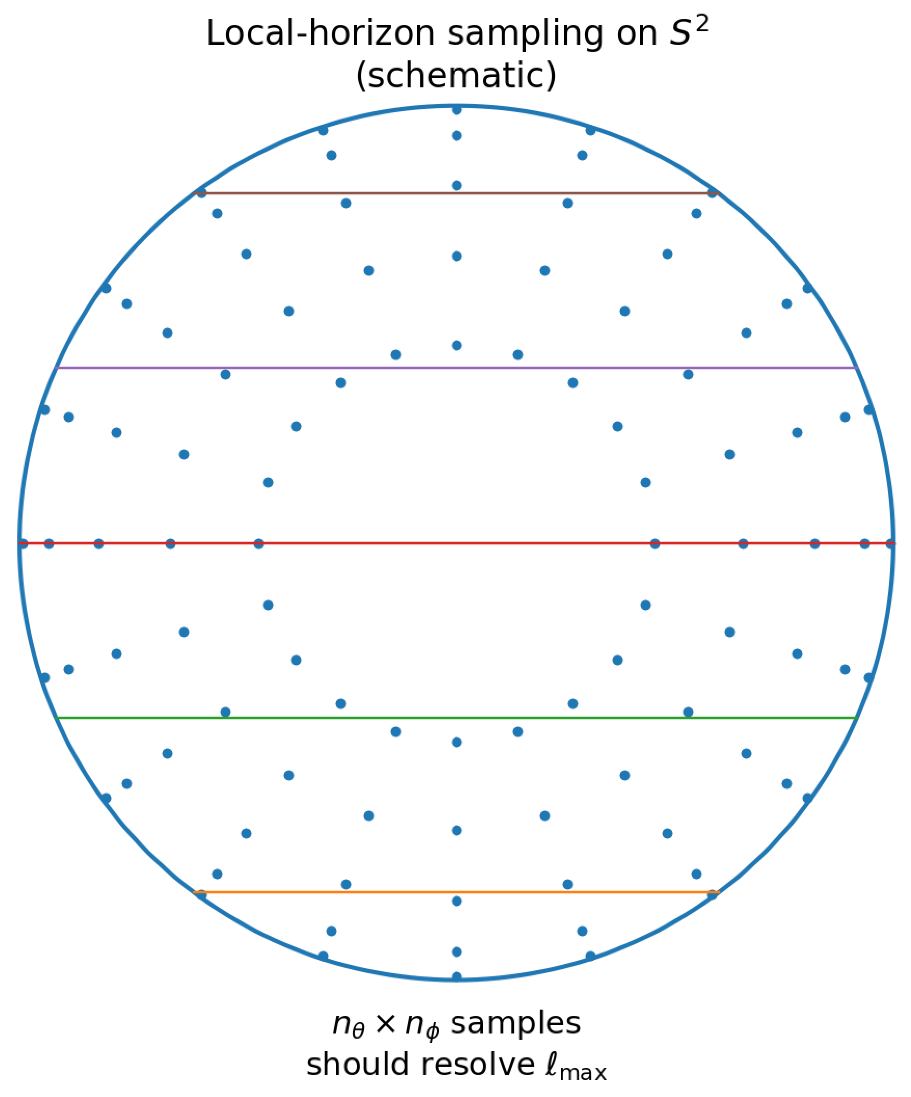
To estimate coefficients reliably, the sampling must resolve the spectral content up to . A practical rule of thumb is
otherwise the discretization itself may introduce aliasing-like distortions in the projected coefficients [15,16]. It is worth stressing the distinction: this is numerical aliasing due to insufficient sampling, whereas the HBMB cutoff is interpreted as a physical bandlimit (in toy form) set by finite horizon capacity.
Figure 2.
Schematic sampling of a local-horizon . The number of samples should be consistent with the angular bandlimit to ensure stable coefficient estimation.
Figure 2.
Schematic sampling of a local-horizon . The number of samples should be consistent with the angular bandlimit to ensure stable coefficient estimation.
4.4. Mode Coefficients and Reconstruction
Let denote spherical harmonics with and . For an angular toy model, the projection coefficients are defined by
The reconstructed field can be written in a general (bulk-capable) form as
where is a radial basis function determined by the background geometry and the chosen boundary conditions. In a pure angular toy model one fixes r (e.g., ) and may simply take .
4.5. Error Metrics
Norms are defined with the appropriate measure. For angular toy models, the norm on is
We define the relative error by
A pointwise (supremum) error metric is
To quantify spectral coverage we use the squared-amplitude sum of coefficients:
where is a large numerical reference cutoff approximating the “nearly complete” spectrum (e.g., the largest ℓ that remains stable for the chosen grid).
Optionally, one may report a shape correlation defined via the inner product
Figure 3.
Conceptual example: reconstruction error typically decreases as increases, i.e., as the cutoff approaches the capacity-implied limit.
Figure 3.
Conceptual example: reconstruction error typically decreases as increases, i.e., as the cutoff approaches the capacity-implied limit.
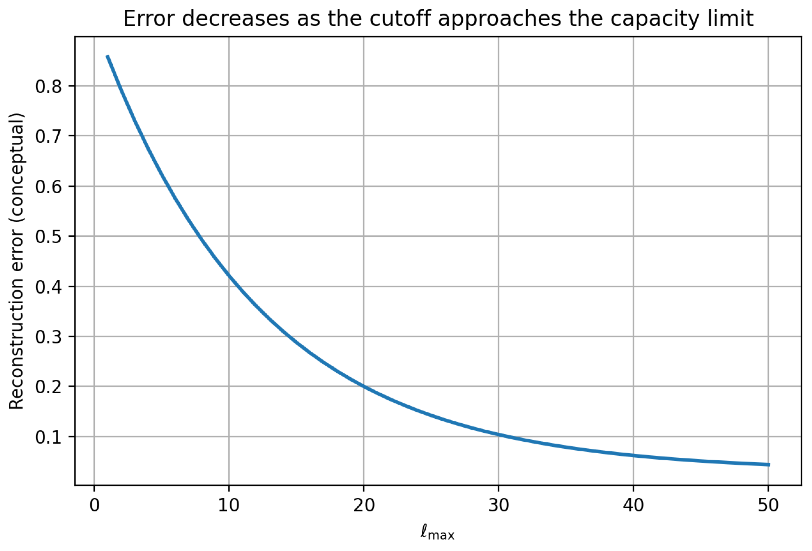
4.6. Scaling Study and Unified Reporting
We run the above steps for multiple cutoff values (e.g., up to the HBMB-implied cutoff) and plot the error metrics as functions of . In a clean toy demonstration, decreases systematically while approaches 1. For sharply localized targets, one may observe ringing/Gibbs-type artifacts at low cutoff, which should weaken as increases.
For each geometry, we will provide a compact summary table reporting: R, , , the basis choice (including where relevant), numerical settings (, and in bulk toy variants), and the primary metrics (, , , optionally ).
5. Flat Spacetime Baseline: Spherical “Screen” Reconstruction + Control Benchmarks (Hydrogen, Stress Test)
In this chapter we run the HBMB holography protocol fixed in Sec. 4 in the simplest possible baseline setting: a flat (Minkowski) background with a spherical screen at fixed radius. The goal is not to model time evolution, but to demonstrate that the pipeline
is numerically stable and that the reconstruction quality is controlled by a capacity-driven cutoff (HBMB), rather than by an arbitrary Fourier truncation.
We then validate the pipeline with analytically controlled targets (hydrogenic angular states) and a high-ℓ stress test showing a sharp threshold behavior: if the target contains a critical component at , then for the reconstruction cannot be accurate, while for the error collapses (numerically) to the floating-point limit.
5.1. Geometric Setup: Spherical Screen in a Flat Background
In the flat baseline, the “boundary” is taken to be a spherical screen at fixed radius R. Its induced angular metric is
The natural eigenbasis is the set of spherical harmonics
which satisfy the orthonormality relation on :
5.2. Target Field on the Screen
As a smooth localized target we use a Gaussian-like “blob” on the sphere. Denoting the great-circle distance by , we have
and the target field is defined by
where is the center of the blob and controls its width.
5.3. HBMB/Bekenstein Cutoff:
The number of angular modes up to is
At the toy level we identify the available independent coefficients with an effective bit-capacity:
Remark (toy vs. physical scales).
In the toy sections, is a dimensionless effective capacity parameter chosen such that the HBMB cutoff lies in a numerically tractable range; for physical horizons one has , which naturally yields enormous values.
In our runs , hence
5.4. Coefficients and Reconstruction
The projection coefficients are
and the truncated reconstruction is
The FAST implementation uses FFT along and Gauss–Legendre quadrature in for the polar integration. This combination is stable and efficient in the parameter ranges considered here.
5.5. Error Metrics and Spectral Coverage
We quantify accuracy by the relative error
and by a max-norm metric (normalized by the target amplitude):
We also track the spectral energy coverage
which is a robust metric motivated by Parseval’s identity on [20].
5.6. Numerical Results: Flat Toy
The flat toy runs show a systematic decrease of reconstruction error with increasing , while the coverage rapidly approaches unity.
Figure 4.
Flat toy: relative error vs. .
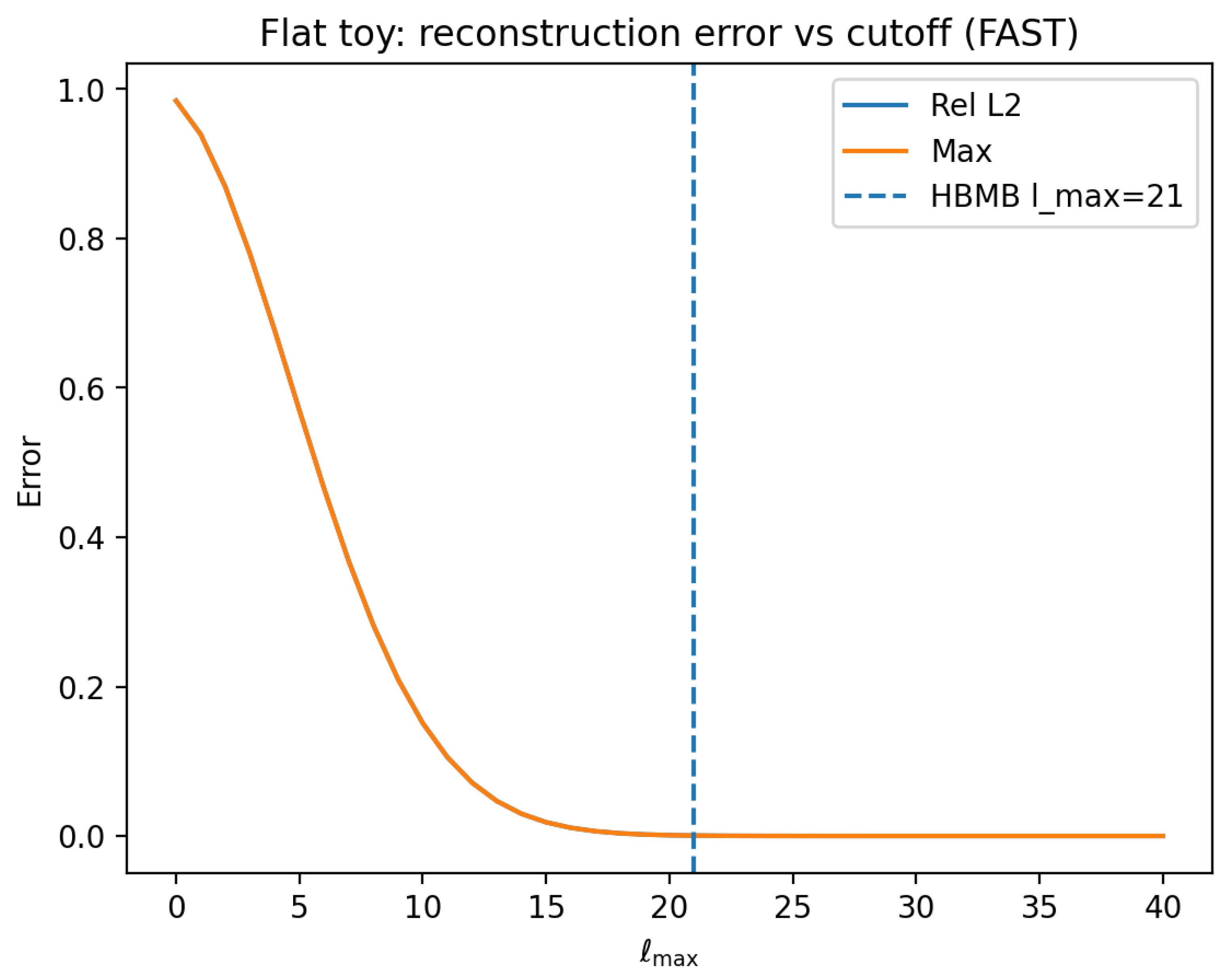
Figure 5.
Flat toy: spectral coverage vs. cutoff.
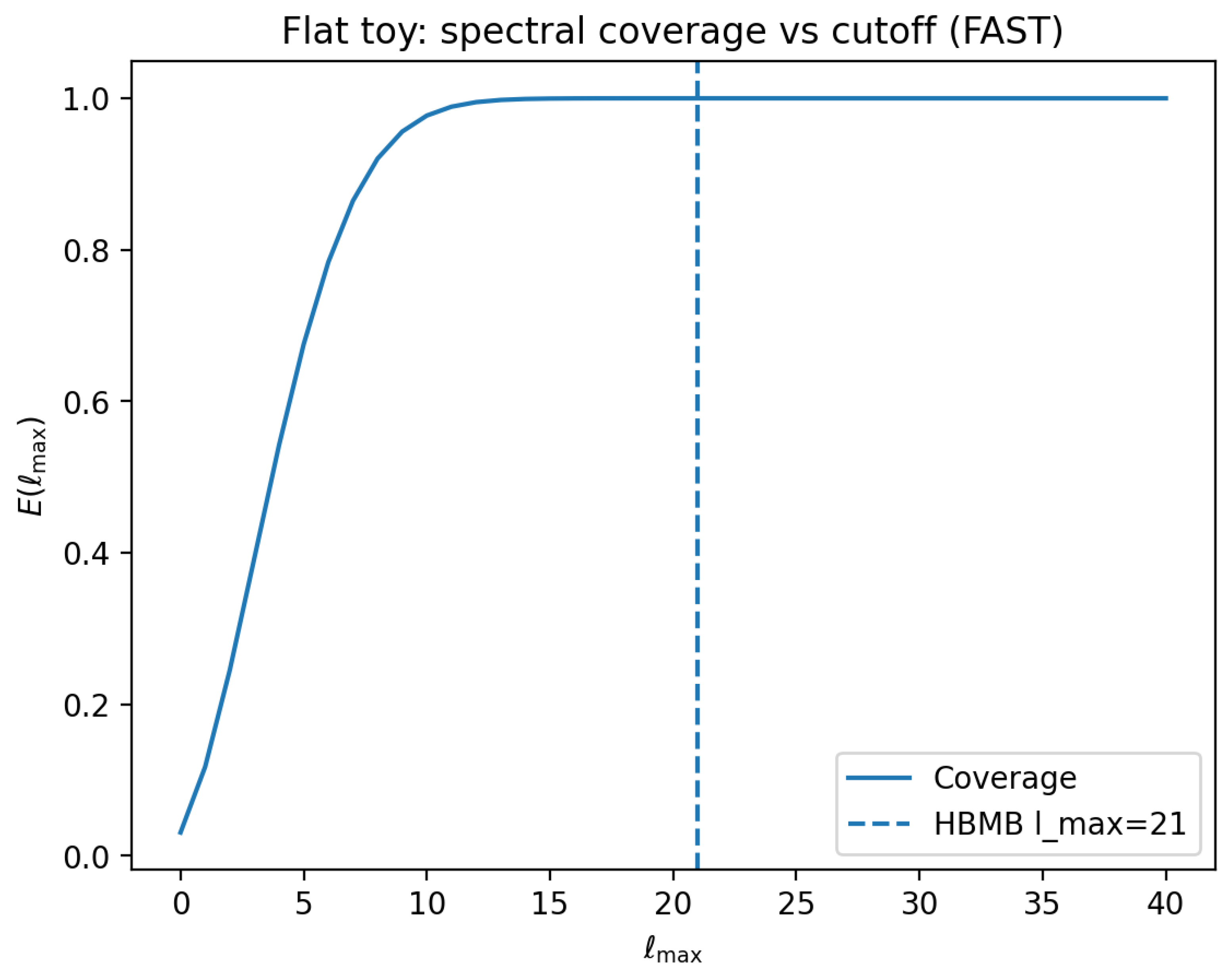
Figure 6.
Flat toy: target vs. reconstruction maps of at .
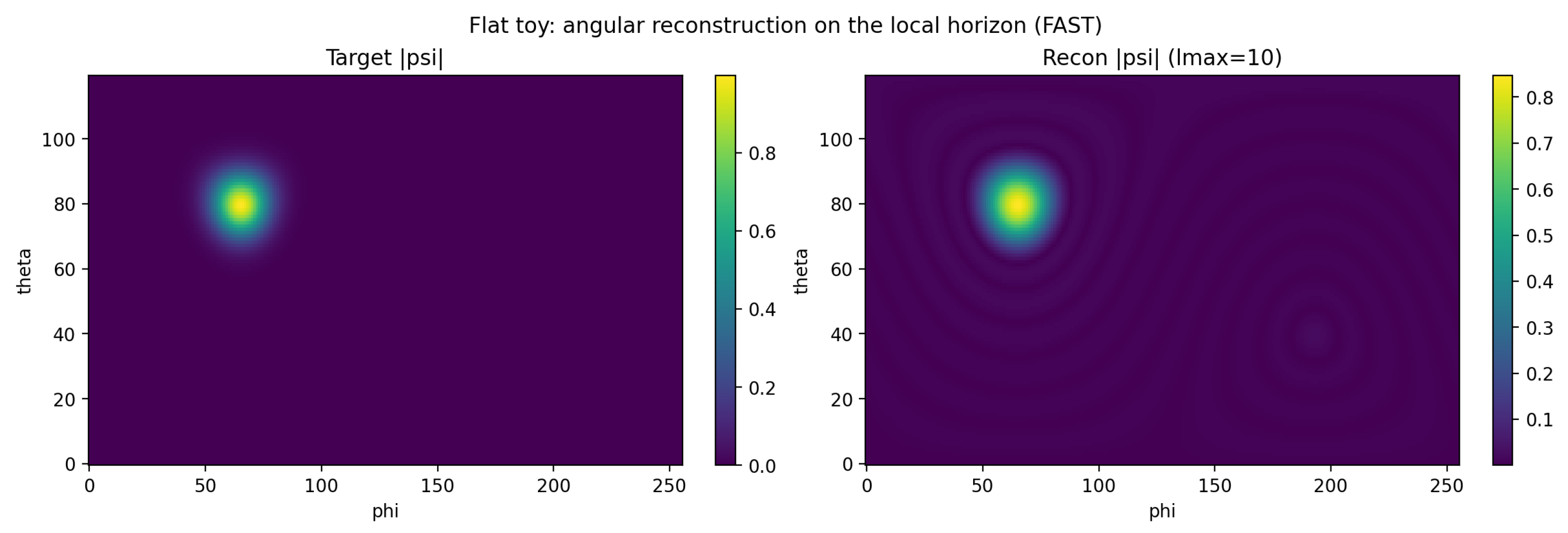
Figure 7.
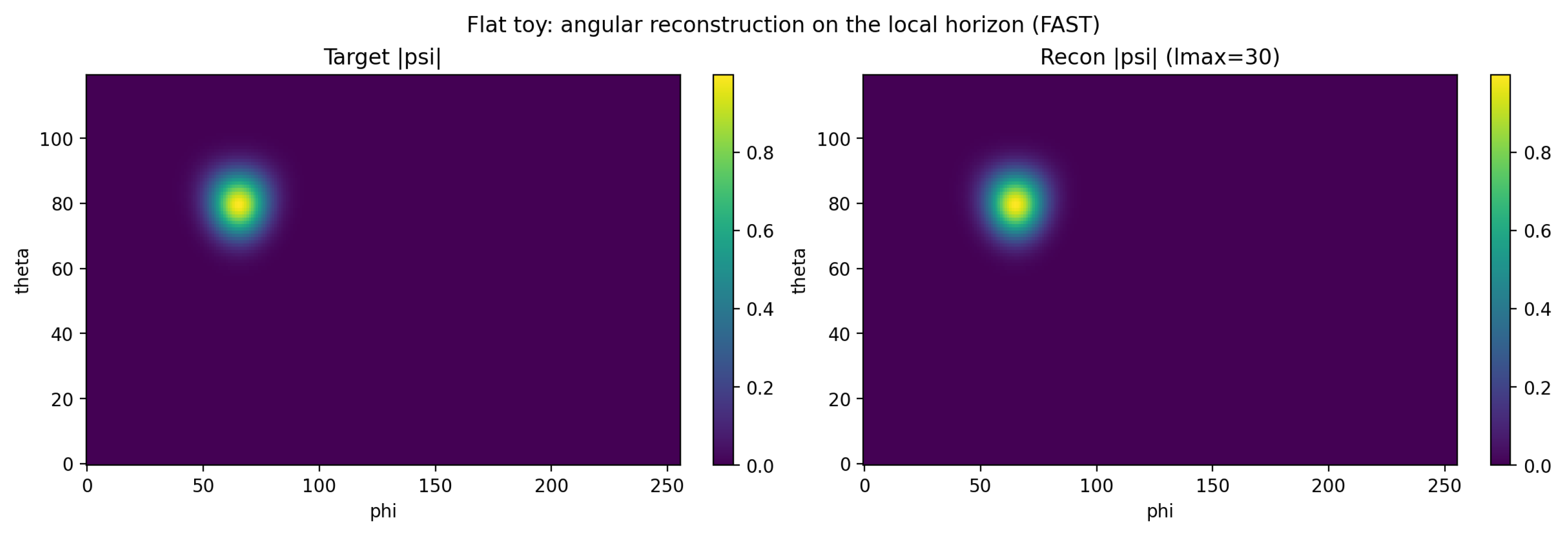
Flat toy: target vs. reconstruction maps of at .
5.7. Hydrogen Control Benchmark: Physical Target and Screen Reconstruction
For a strong validation we use targets with analytically known angular structure. For hydrogenic orbitals,
Restricting to a fixed r (i.e., to the screen) yields an angular target that is a finite linear combination of spherical harmonics:
This is an ideal control: once covers the highest excited , the reconstruction closes to floating-point precision.
Figure 8.
Hydrogen control (flat): relative error vs. .
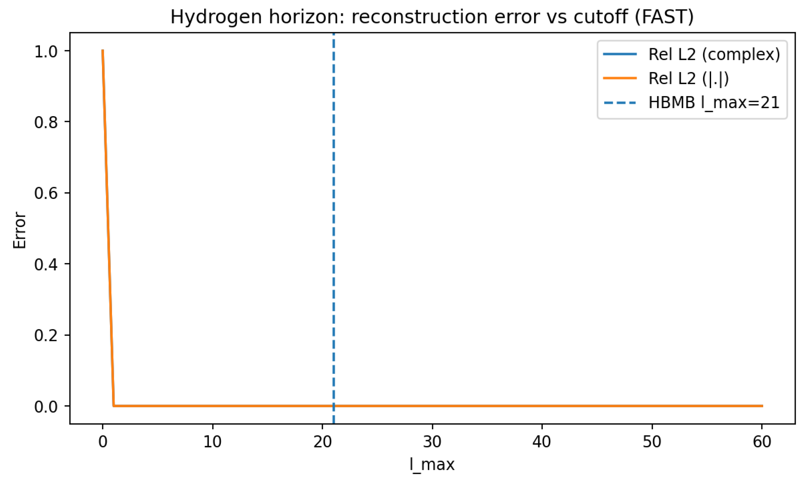
Figure 9.
Hydrogen control (flat): spectral coverage .
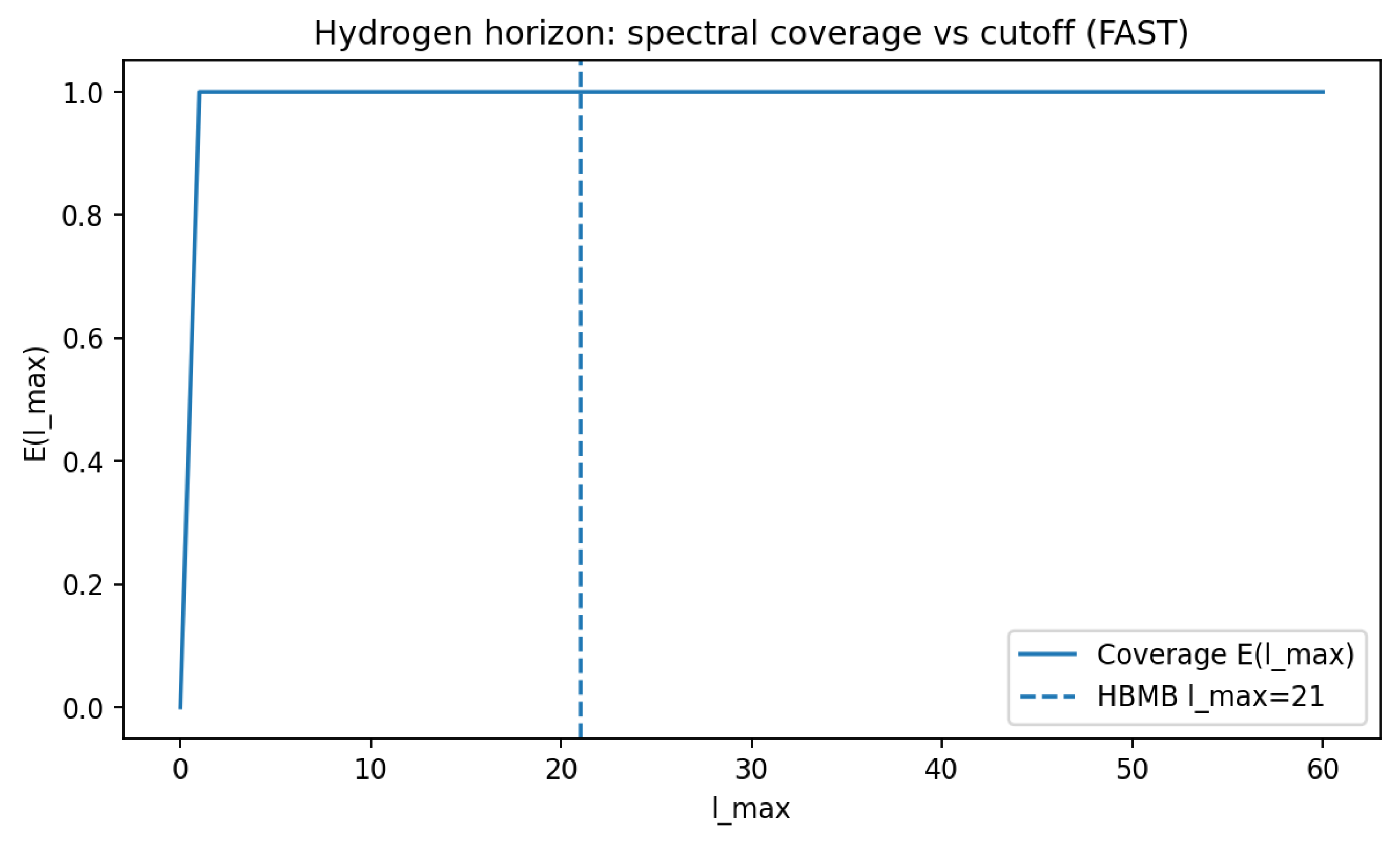
Figure 10.
Hydrogen control: on the screen.
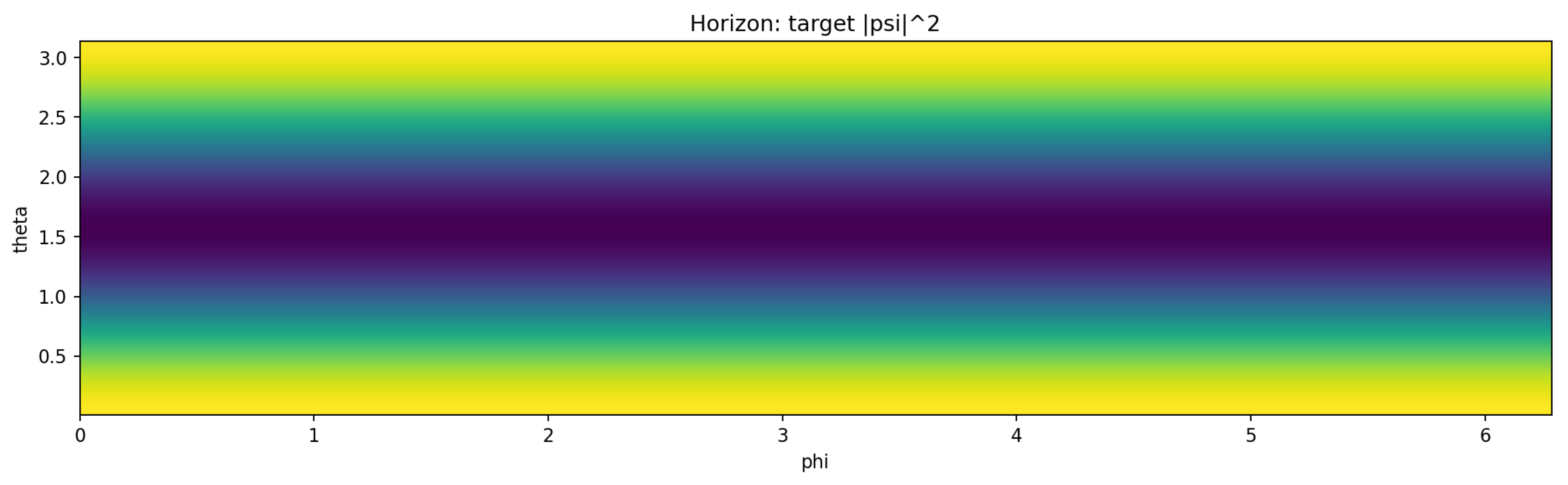
Figure 11.
Hydrogen control: reconstructed at .
5.8. Superposition Test: Complex Weights and Interference (Flat)
Next we test phase-correctness by reconstructing a complex superposition:
By linearity of the projection and synthesis maps,
so agreement at the complex-field level demonstrates that HBMB reconstructs not only amplitudes but also phases (i.e., interference structure).
Figure 12.
Superposition test (flat): relative error vs. .

Figure 13.
Superposition test (flat): spectral coverage .
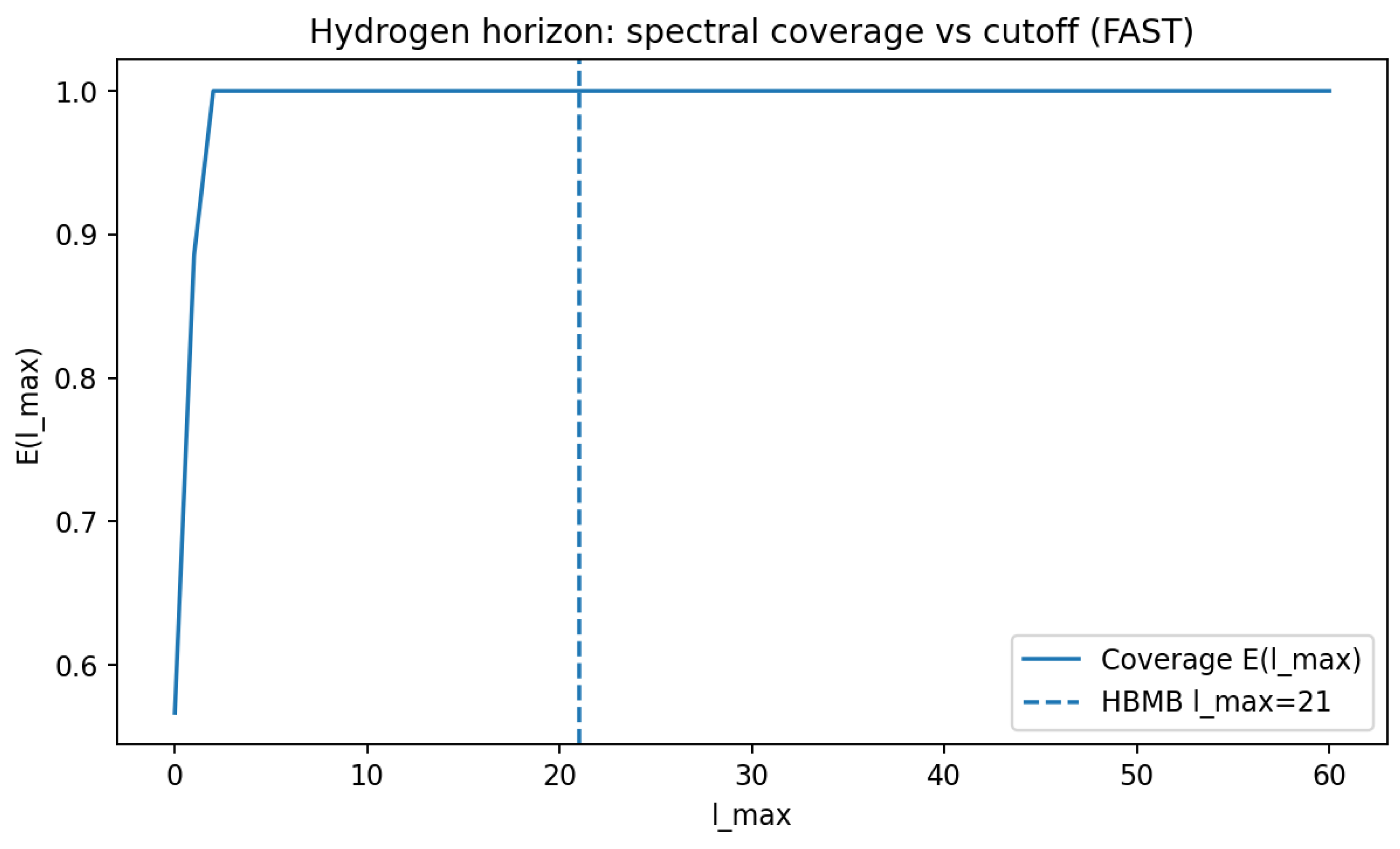
Figure 14.
Superposition test: phase map on the screen.
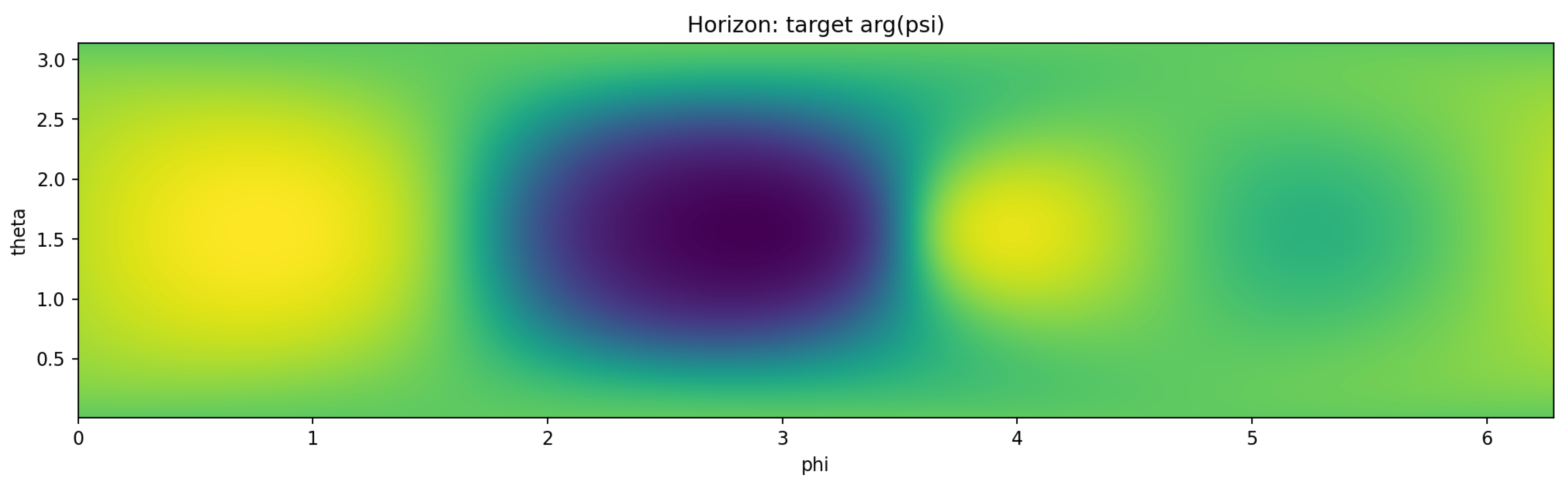
Figure 15.
Superposition test: reconstructed phase map at .
5.9. High-ℓ Stress Test: Sharp Evidence for Cutoff Logic (Flat)
In the stress test we choose a target with an explicit critical high-ℓ component. Let and . We define
HBMB predicts a sharp threshold:
The same behavior appears in the coverage metric as a jump of to unity at the critical cutoff.
Figure 16.
High-ℓ stress test: power distribution of the target spectrum in the plane, highlighting the critical component.
Figure 16.
High-ℓ stress test: power distribution of the target spectrum in the plane, highlighting the critical component.
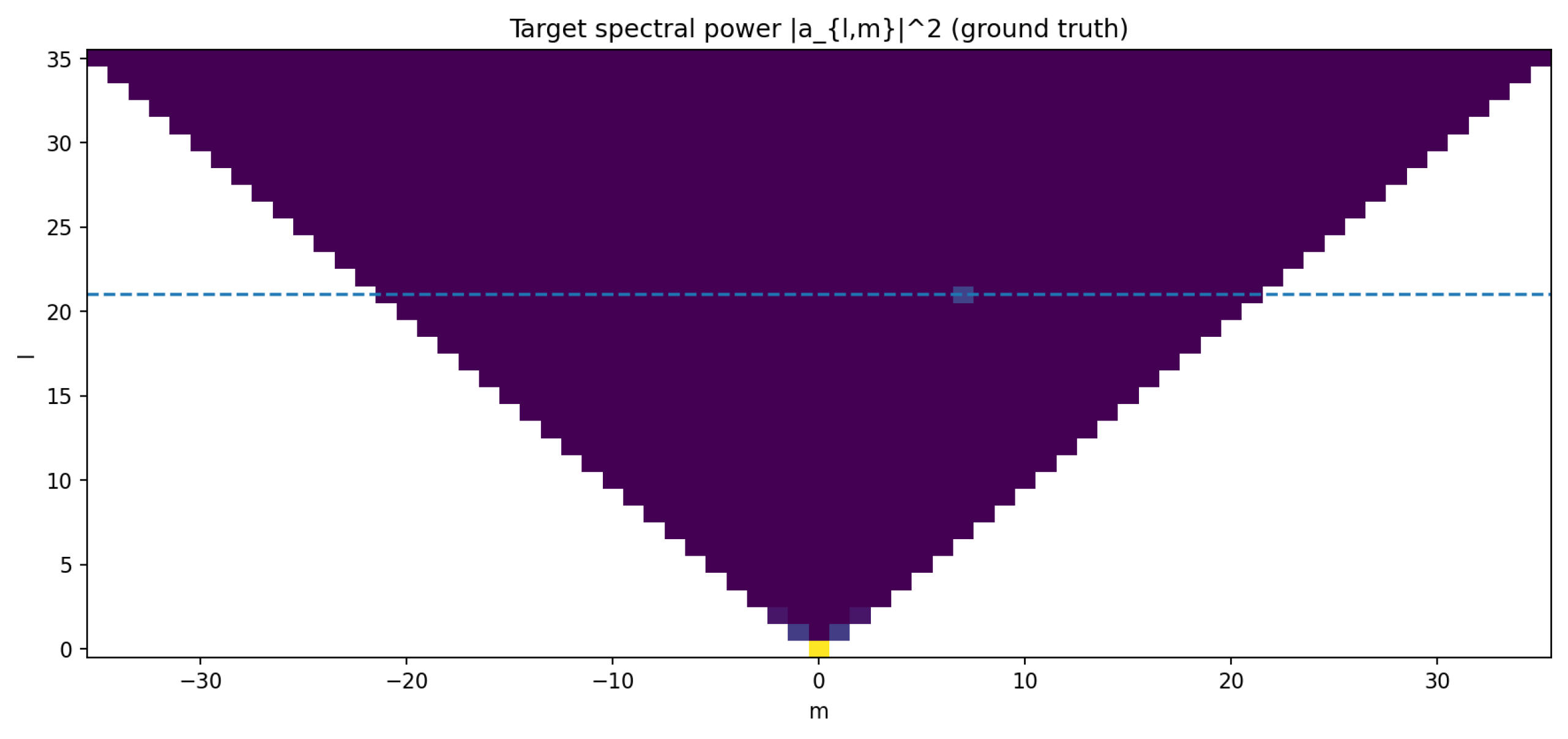
Figure 17.
High-ℓ stress test: reconstruction error vs. . The error collapses at .
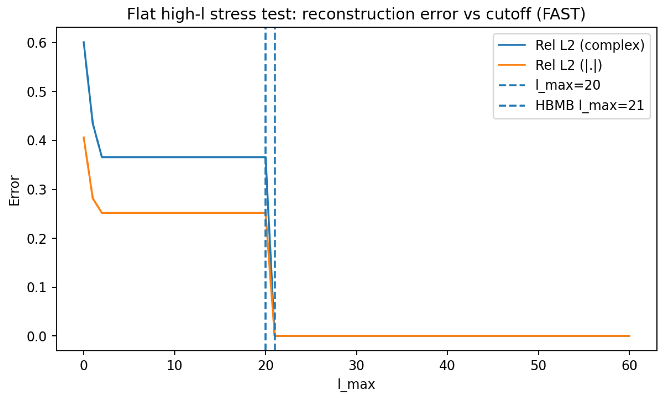
Figure 18.
High-ℓ stress test: coverage jumps to 1 at the critical cutoff.
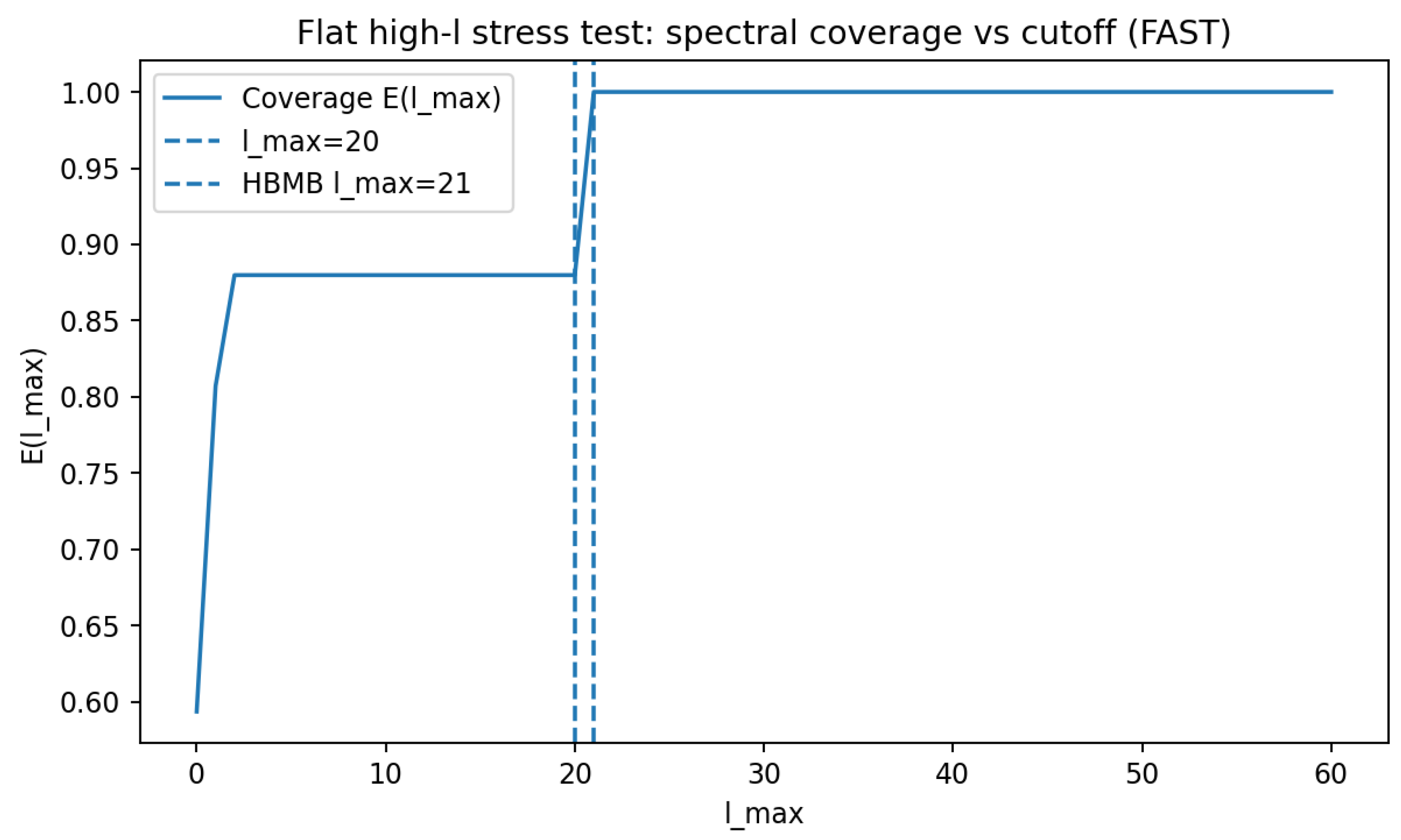
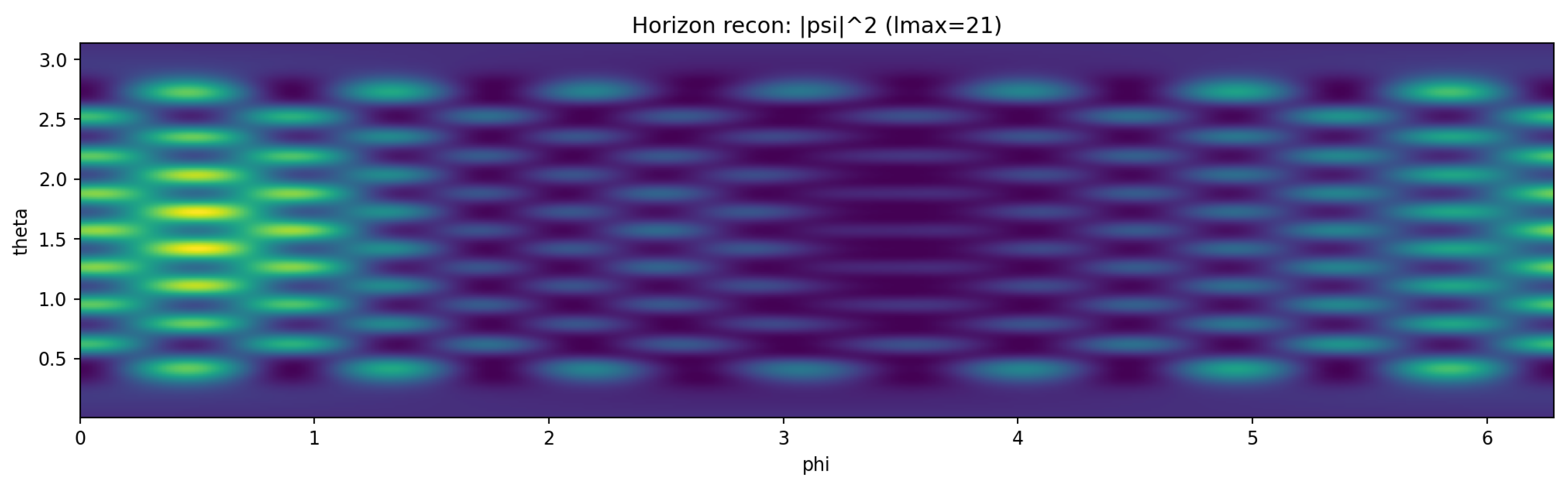
Figure 19.
High-ℓ stress test: reconstructed at (the critical mode is still missing).

Figure 20.
High-ℓ stress test: reconstructed at (the critical mode enters and the structure appears).
Figure 20.
High-ℓ stress test: reconstructed at (the critical mode enters and the structure appears).

5.10. Summary: What Does the Flat Baseline Establish?
The main takeaways of the flat baseline are:
- Hydrogen controls close to machine precision, validating the projection+synthesis pipeline.
6. dS Toy Model: Local-Horizon Eigenmode Reconstruction + Control Benchmarks (Hydrogen, Stress Test)
In this chapter we run the HBMB holography protocol fixed in Sec. 4 on an explicit local (spherical) horizon in a de Sitter (dS) static-patch angular toy setting. The aim here is not to model full dS dynamics (time evolution), but to demonstrate that boundary data stored on a local dS cosmological horizon—represented by the mode coefficients —suffice to reconstruct the bulk field’s angular dependence (first, on the horizon itself) via a truncated eigenmode synthesis, and that the reconstruction quality is controlled by a capacity-driven physical cutoff, rather than a mere numerical convenience.
We then provide strong validation using control benchmarks: hydrogenic angular states are ideal because the eigenbasis (spherical harmonics) is analytically known. Finally, a high-ℓ stress test shows that the cutoff logic is sharp: if the target contains a critical component at , then for the reconstruction cannot be accurate, while for the error collapses (numerically) to the floating-point limit.
6.1. Geometric Setup: dS Static Patch and a Local Horizon
In four dimensions, the de Sitter metric in static coordinates reads [17]:
where R is the dS curvature radius, and
The cosmological horizon of a static observer is located at
with induced angular geometry .
In the present toy demonstration we focus on angular reconstruction: we fix r close to the horizon (numerically, often with ), so the reconstruction effectively reduces to an eigenmode synthesis on .
6.2. Target Field Choice: What Is ?
We choose a target field such that it (i) excites multiple ℓ-bands (to make the cutoff effect visible) and (ii) remains numerically stable under projection (quadrature + FFT). Typical choices include:
- a localized Gaussian “spot” on the sphere (broad ℓ-spectrum),
- sums of multiple spots (interference patterns),
- directly prescribed spectra (control targets).
6.3. HBMB/Bekenstein Cutoff:
For a spherical local horizon, the area is
and the associated (Bekenstein–Hawking / Gibbons–Hawking) entropy is [1,2,17]
At toy level we identify the horizon bit-capacity with this quantity:
In a spherical-harmonic basis, the number of angular modes up to is
The HBMB toy postulate ties available independent mode coefficients to capacity,
yielding the cutoff estimate
In our numerical runs we worked with dimensionless toy parameters (effectively and an ), for which
matching the code output HBMB l_max=21.
Remark (toy vs. physical scales).
In the toy sections, is a dimensionless effective capacity parameter chosen such that the HBMB cutoff lies in a numerically tractable range; for physical horizons one has , which naturally yields enormous values.
6.4. Mode Coefficients and Reconstruction
The horizon projection coefficients are defined by
The truncated reconstruction is
FAST implementation (numerics). We use FFT in the direction and Gauss–Legendre quadrature in for the polar integral. Sampling must be consistent with the reference bandlimit to avoid aliasing. In practice we follow the Nyquist/Shannon intuition [15,16]:
Typical runs used and , supporting a reference with projection times – s.
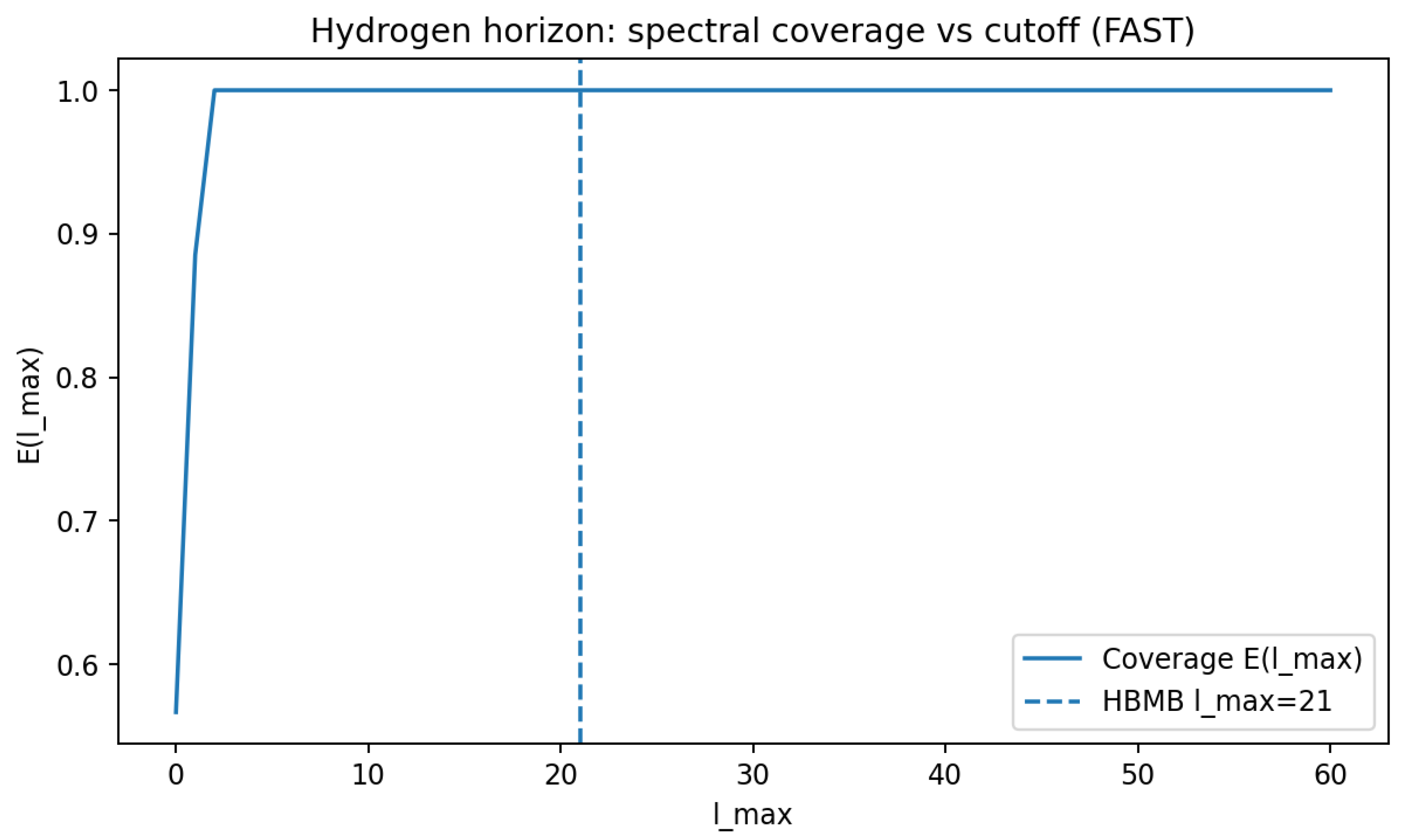
6.5. Error Metrics and “Success” Criteria
We quantify reconstruction quality using the relative error and the spectral coverage (Sec. 4.5). For convenience we restate:
and
Analytic backbone (Parseval on ). Orthonormality of implies [20]
If we define the truncated field by retaining only modes, then the squared relative truncation error is
where the final step uses a large enough reference bandlimit . This explains why the error and coverage curves are tightly linked in the numerical results.
We call the reconstruction successful if decreases systematically as increases while . For control targets that are effectively bandlimited, the error should drop to the floating-point limit as soon as reaches the target’s highest excited ℓ.
6.6. Numerical Results: dS Angular Toy
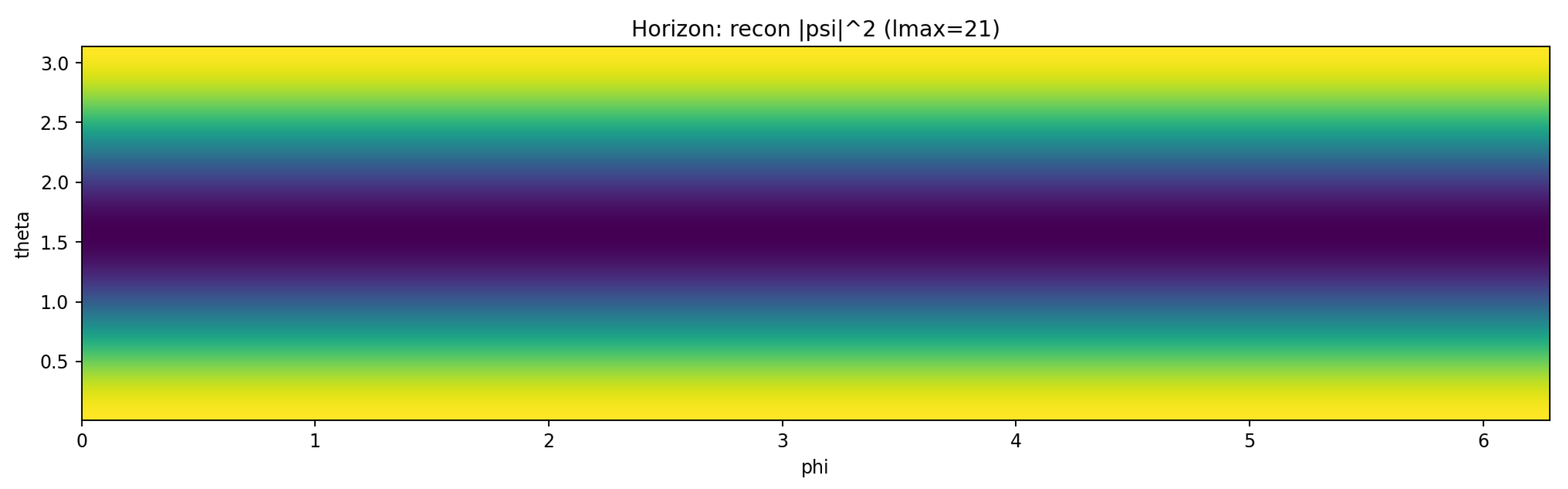
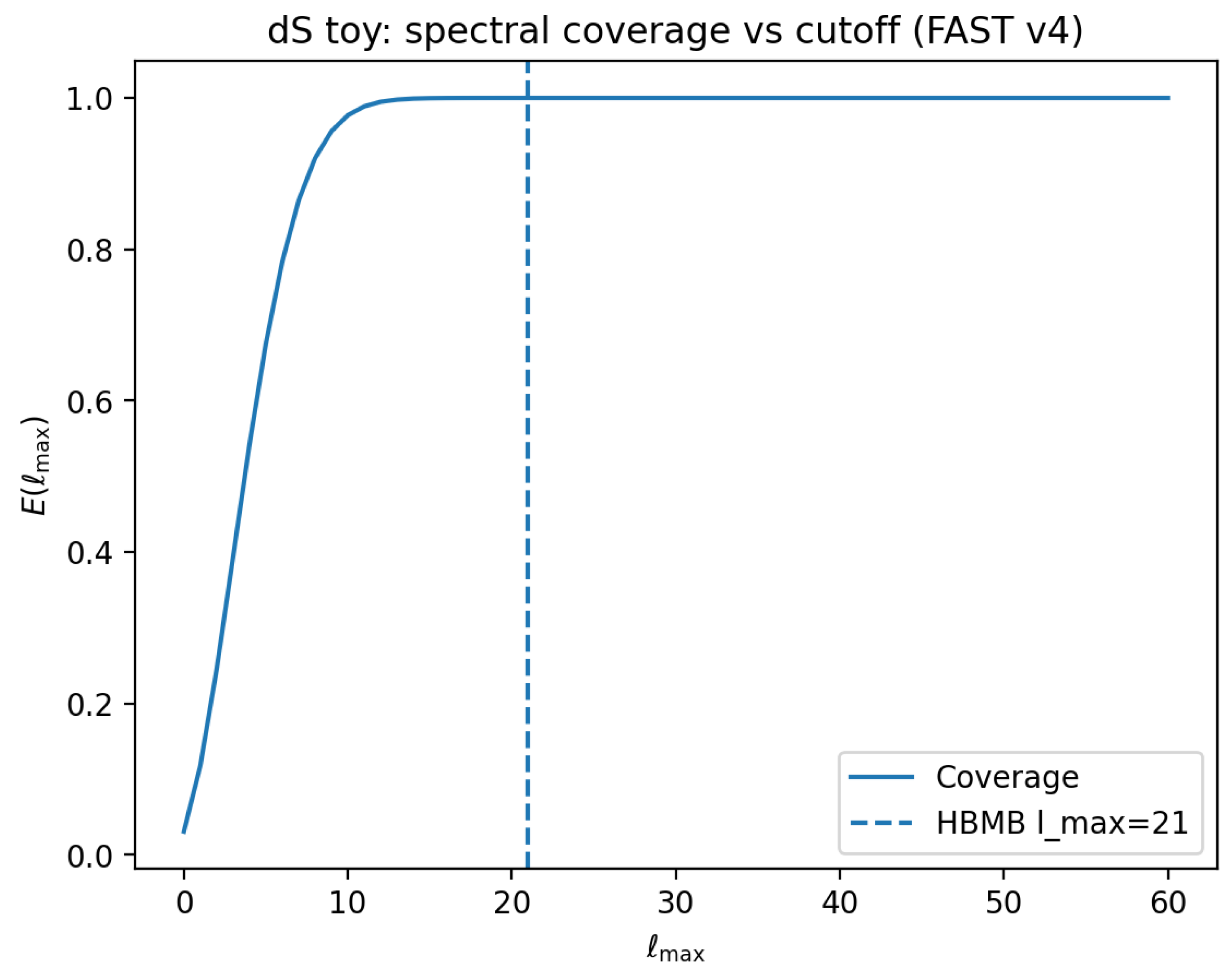
The dS angular-toy runs show that the reconstruction error decreases rapidly with increasing , while the spectral coverage quickly approaches unity.
Figure 21.
dS angular toy: reconstruction error vs. . The HBMB cutoff increase drives systematic convergence.
Figure 21.
dS angular toy: reconstruction error vs. . The HBMB cutoff increase drives systematic convergence.
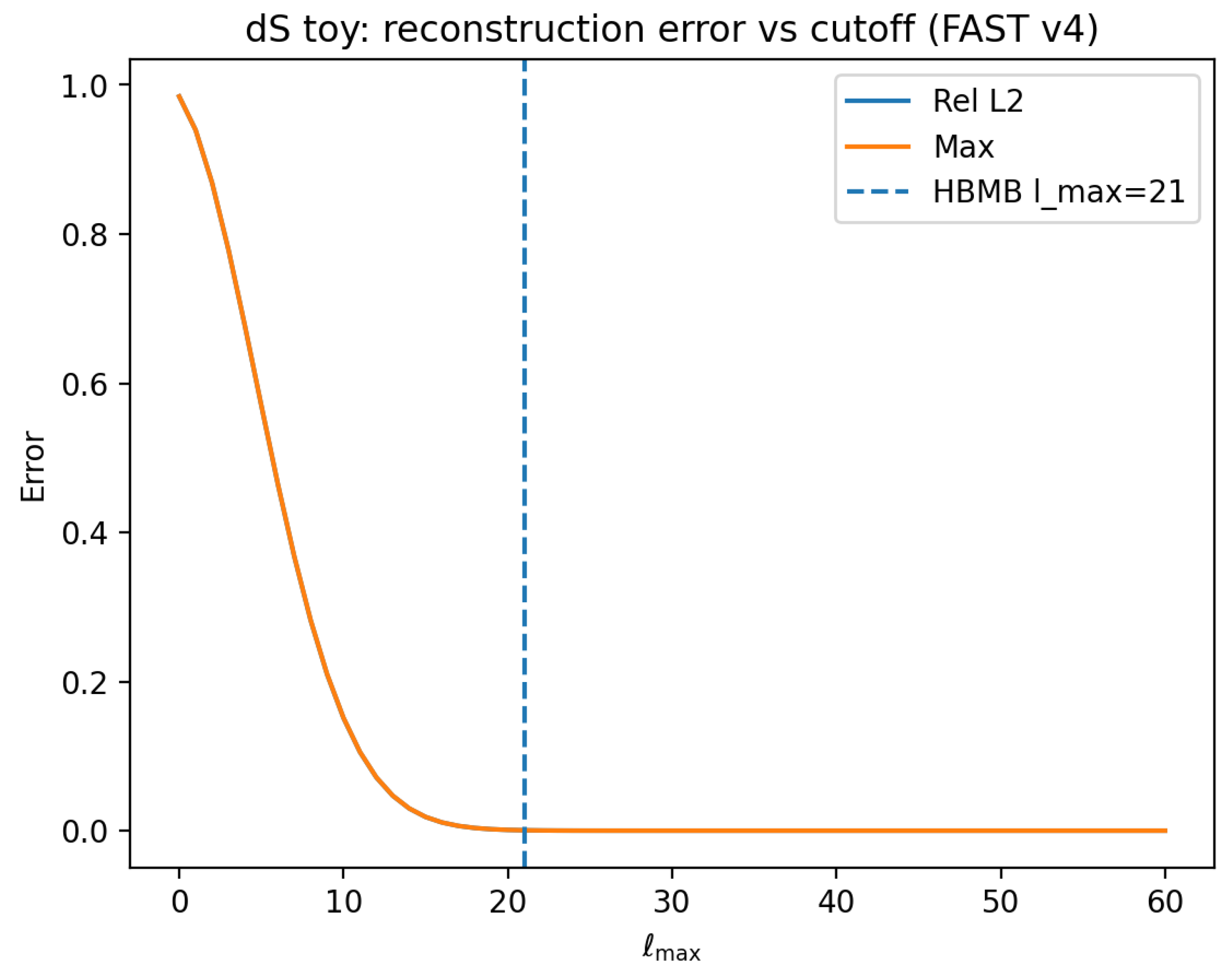
Figure 22.
dS angular toy: spectral coverage . Coverage quickly approaches 1 as the cutoff expands.
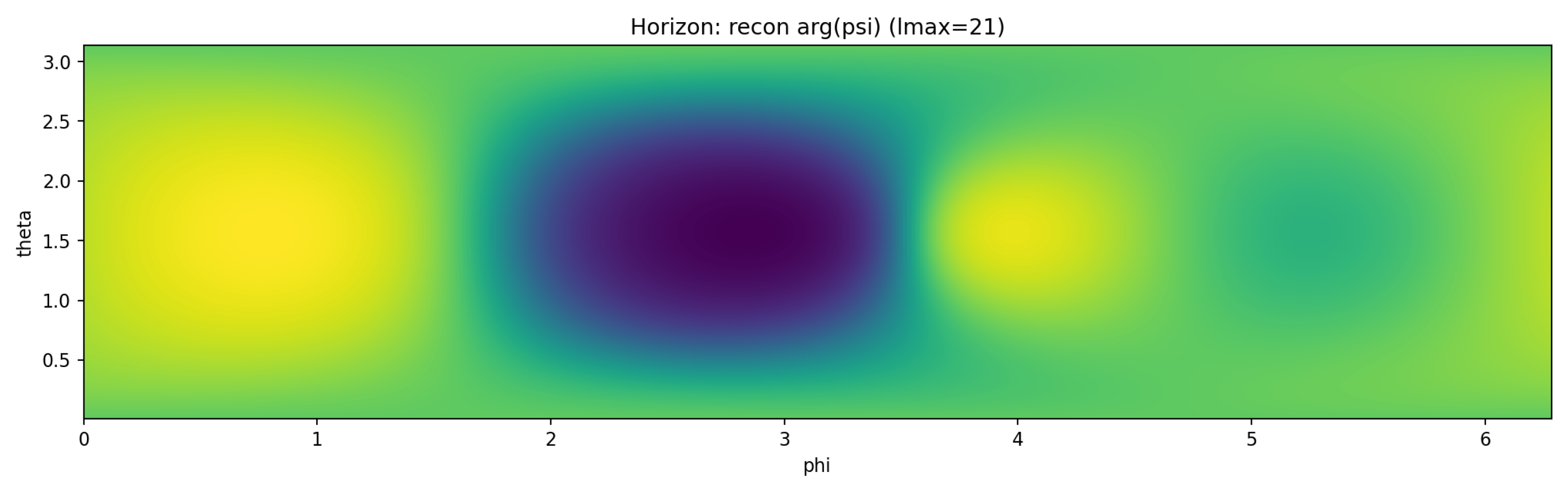
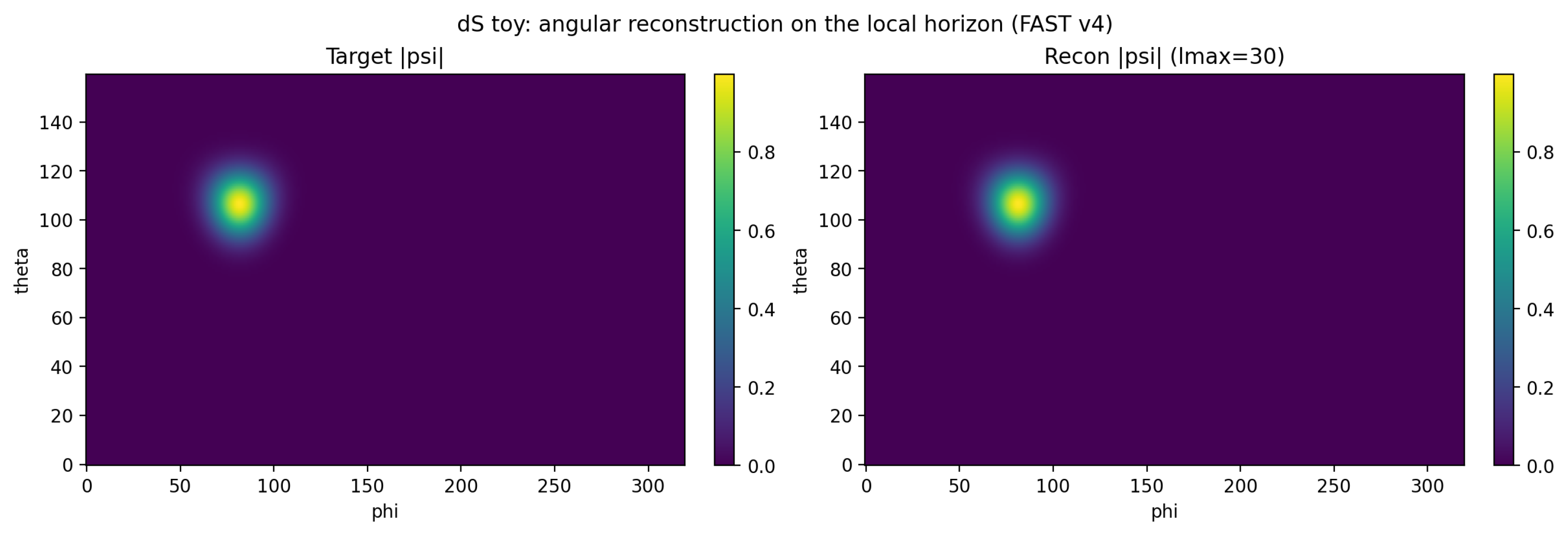
Representative target vs. reconstruction maps at different cutoffs (e.g., and ):
Figure 23.
dS angular toy: maps for target and reconstruction at .
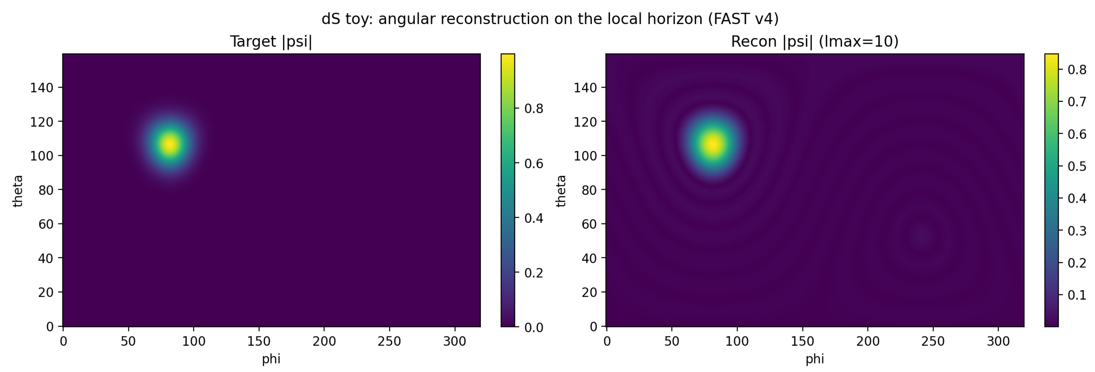
Figure 24.
dS angular toy: maps for target and reconstruction at .
6.7. Hydrogen Control Benchmark: Physical Target and Horizon Reconstruction
We next run the same HBMB pipeline as a control benchmark where the target field has a physically standard form (hydrogenic angular states) and the eigenbasis is analytically known. The goal is that projection + synthesis closes numerically: if the target spectrum lies within , the residual error is set by floating-point precision.
In the run with and , the typical sanity check is
Figure 25.
Hydrogen control: reconstruction error vs. . The error drops to numerical limits once the necessary spectral content is included.
Figure 25.
Hydrogen control: reconstruction error vs. . The error drops to numerical limits once the necessary spectral content is included.
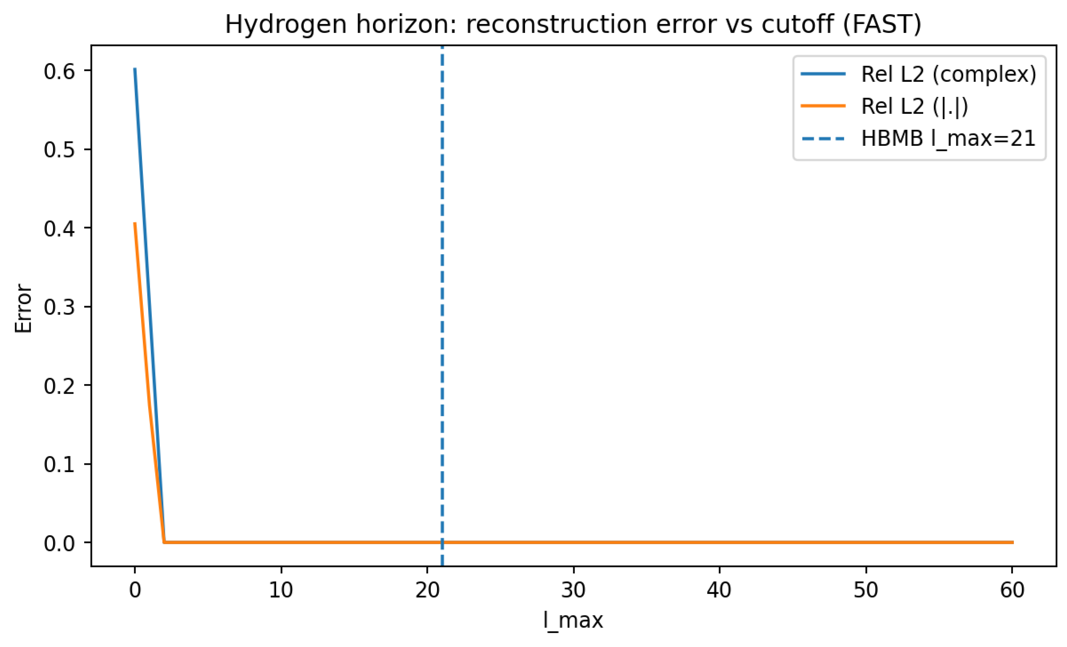
Figure 26.
Hydrogen control: spectral coverage .
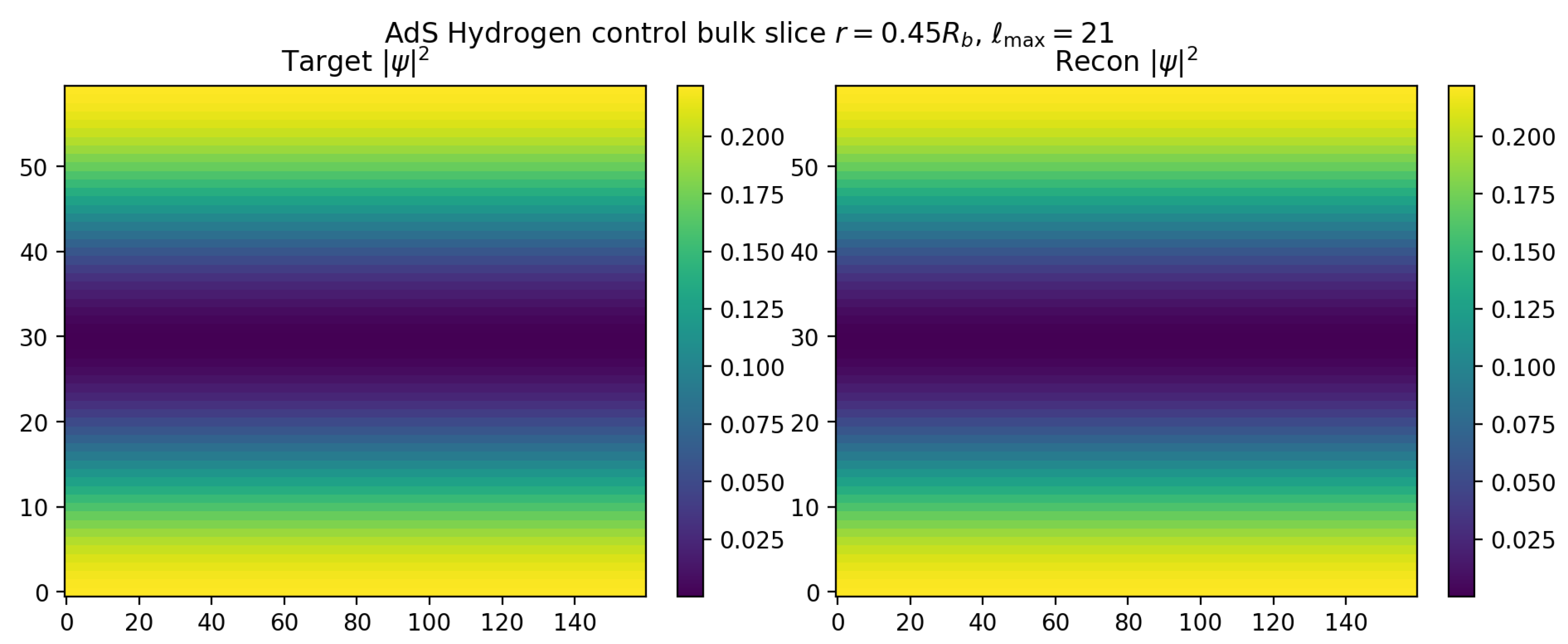
6.8. “Bulk” Extension: Toy Kernel and Bulk Slices
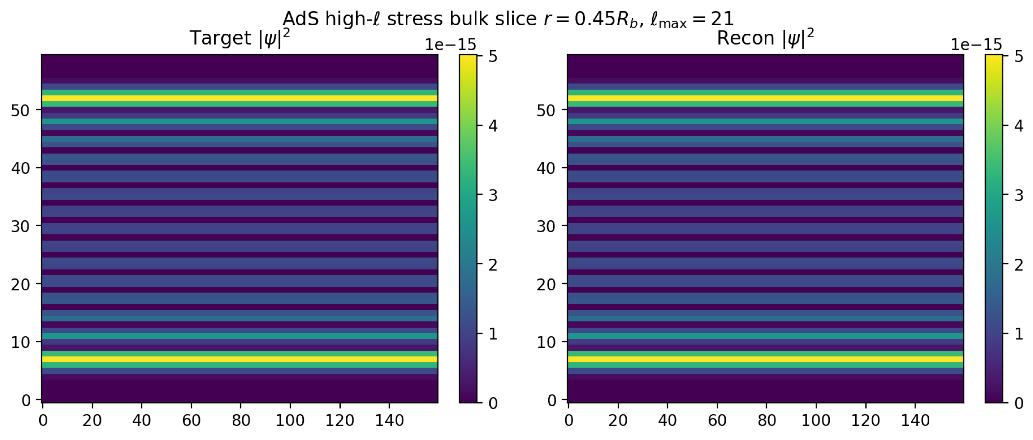
In this chapter, “bulk” is not a full dS dynamical evolution but a simple mode-diagonal radial extension using a toy kernel:
This mimics Poisson/harmonic behavior: higher-ℓ components decay faster away from the boundary. The key point is that the boundary data are unchanged, and the HBMB cutoff still controls angular resolution. Typical slice plots appear as bulk_target_abs2_r*.png and bulk_recon_abs2_r*_lmax21.png.
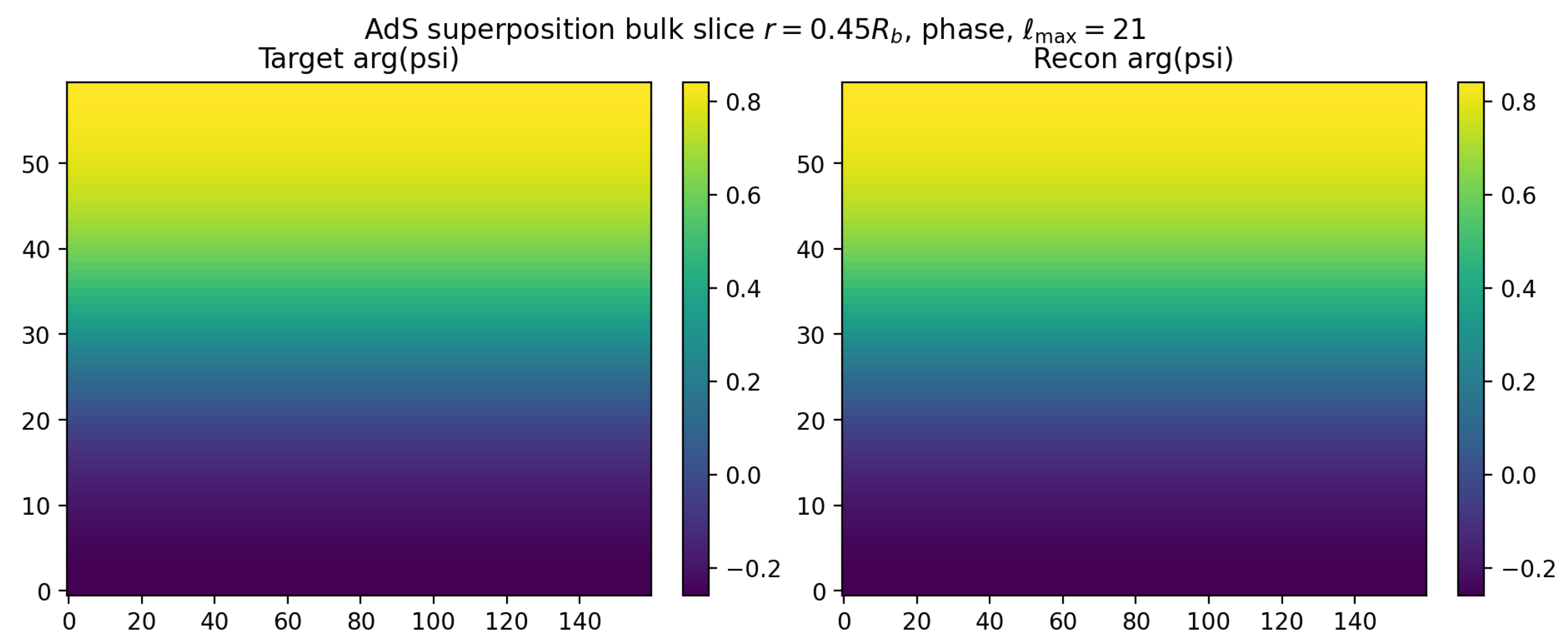
6.9. Superposition test: complex weights and phase correctness
The HBMB pipeline is linear. If the target is a complex superposition, projection and reconstruction must be phase-correct. We test targets of the form
and verify agreement both in magnitude and complex phase (optionally via phase maps ).
6.10. High-ℓ Stress Test: A Sharp Demonstration of Cutoff Logic
To demonstrate that the HBMB cutoff is not a “nice Fourier trick” but a genuine capacity constraint, we build a target containing an explicit critical high-ℓ component. Choose , , and define
with .
HBMB predicts that for the critical mode is outside the allowed capacity, hence the reconstruction error cannot drop; at the mode enters, and the error collapses to numerical precision.
Figure 27.
High-ℓ stress test: reconstruction error vs. . The error stays high for and collapses at (numerically).
Figure 27.
High-ℓ stress test: reconstruction error vs. . The error stays high for and collapses at (numerically).
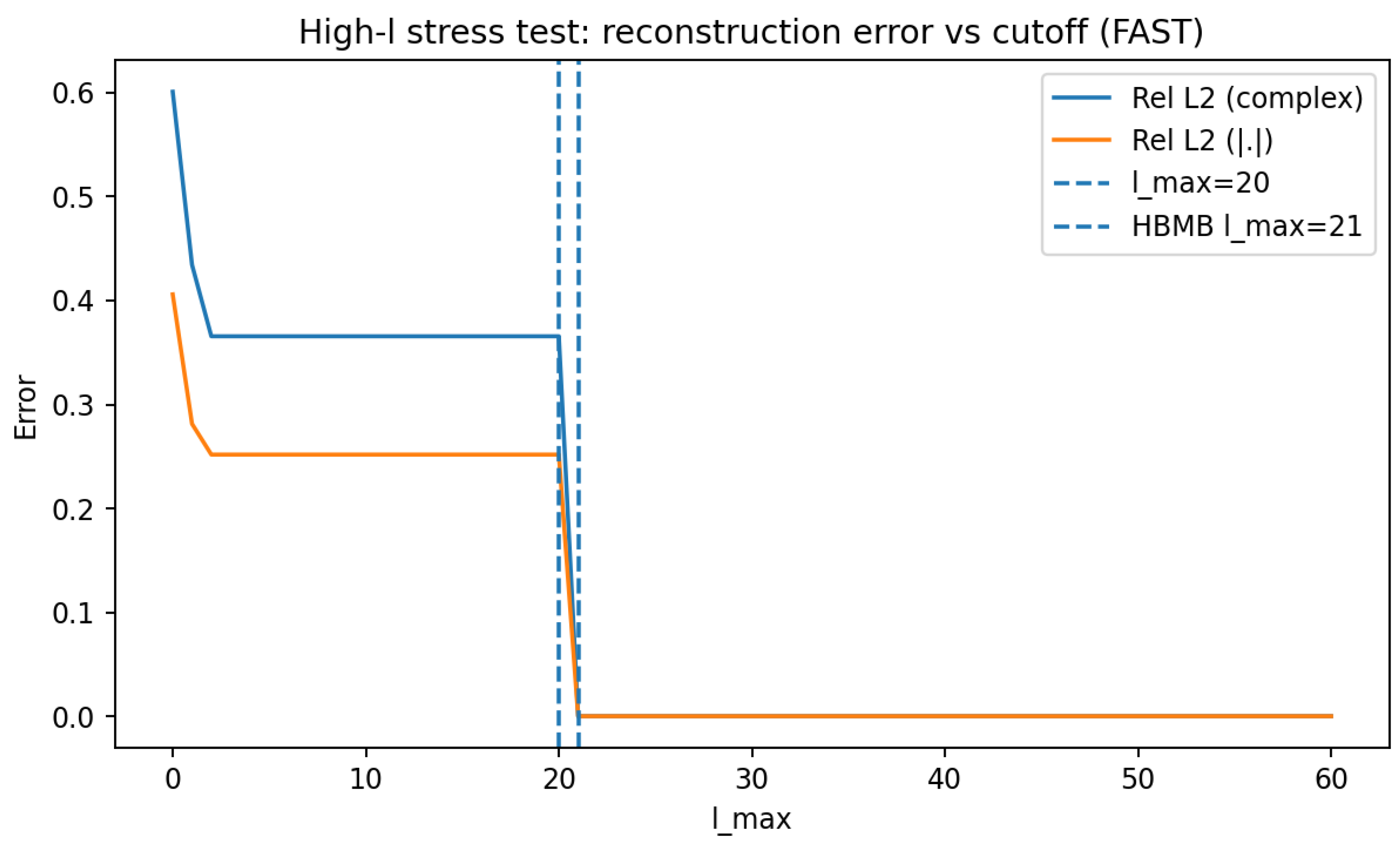
Figure 28.
High-ℓ stress test: spectral coverage . Coverage jumps to unity at the critical cutoff.
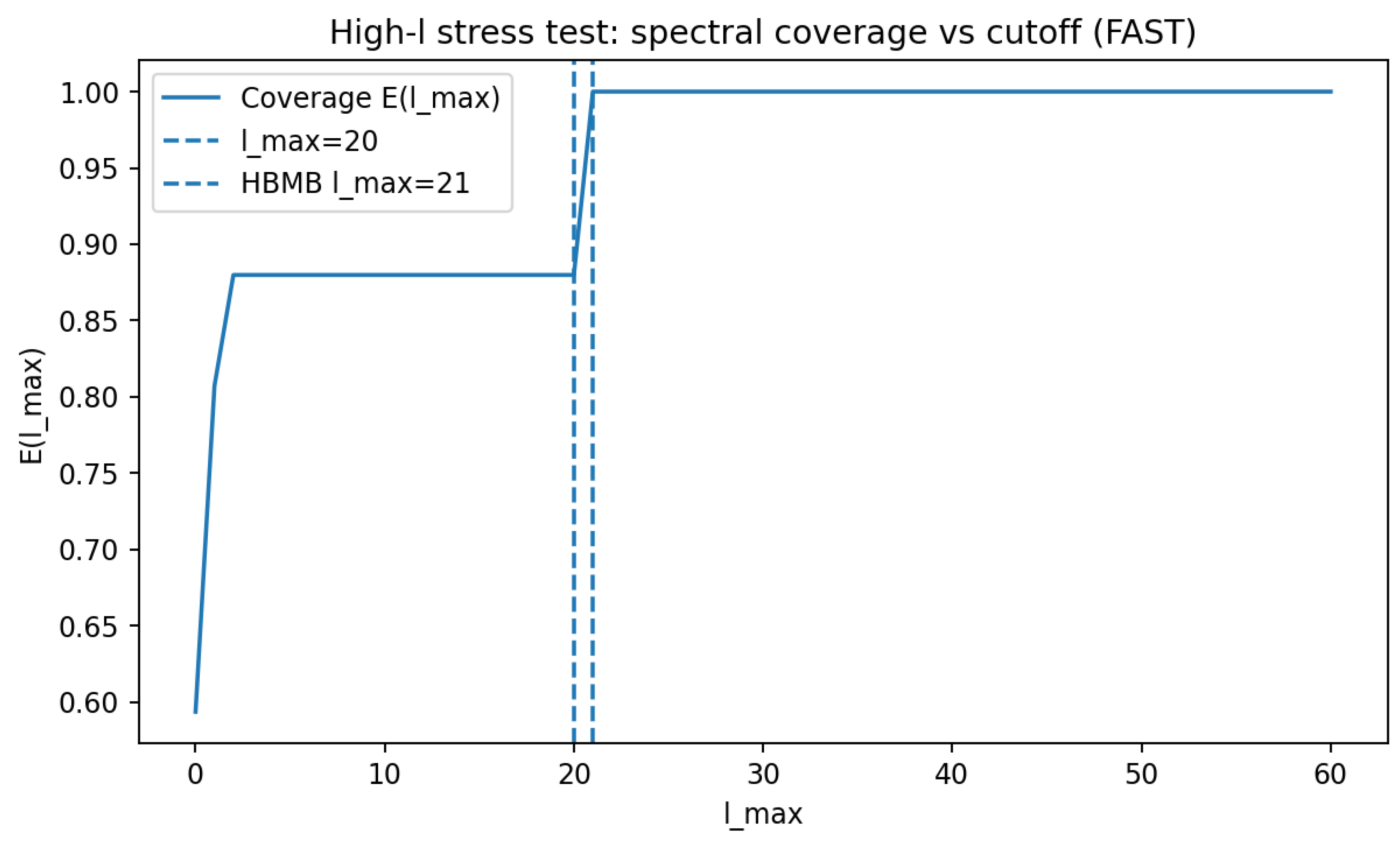
Figure 29.
High-ℓ stress test: reconstruction at (the critical mode is still missing).
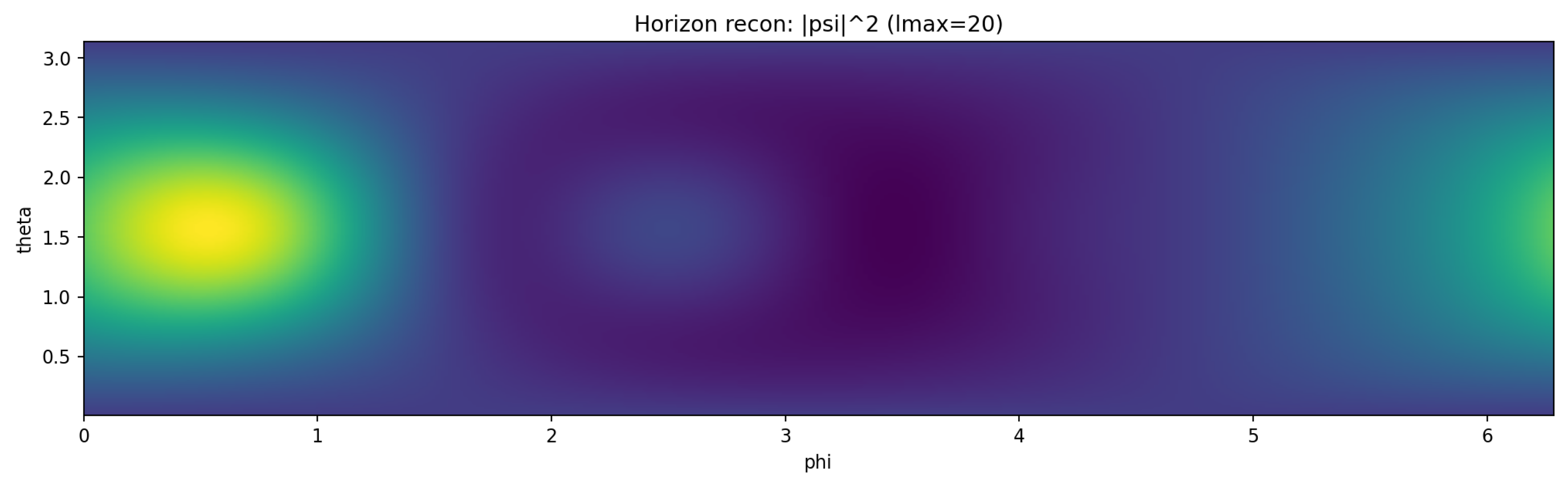
Figure 30.
High-ℓ stress test: reconstruction at (the critical mode enters and the structure appears).
Figure 30.
High-ℓ stress test: reconstruction at (the critical mode enters and the structure appears).
6.11. Summary: Key Outcomes of this Chapter
- The HBMB toy protocol on a dS static-patch horizon is numerically stable and fast (FAST: FFT + Gauss in ), and the reconstruction converges with increasing .
- Hydrogen control benchmarks close to machine precision, strongly validating the correctness of the projection and reconstruction pipeline.
- The toy “bulk” extension via a mode-diagonal kernel remains consistent; the boundary data still control the bulk slices, and the cutoff governs angular resolution.
7. AdS Toy Model: Bulk Reconstruction from a Local Boundary/Screen and HKLL Comparison
In this chapter we run the HBMB-holography protocol in a (toy) anti-de Sitter background, using boundary/screen data to reconstruct a bulk slice (at fixed ). The AdS case is particularly important because the standard holography literature (AdS/CFT) and the HKLL-type bulk reconstruction (“smearing”) formalism provide a natural reference point [21,22,23,24,25]. The goal is twofold: (i) to demonstrate that HBMB-cutoff-controlled convergence works in AdS exactly as in the flat/dS cases, and (ii) to explicitly compare HBMB eigensynthesis to the mode-space form of HKLL smearing.
7.1. Geometric Setup: Static AdS Patch and the Chosen Screen
For context, consider AdS4 in static coordinates:
where L is the AdS curvature radius. In the toy protocol, “boundary data” are taken on a fixed-radius sphere,
(a numerically convenient “cutoff boundary”), and we reconstruct the bulk field on an interior slice .
The angular eigenbasis is the same as before:
with orthonormality
7.2. Mode Expansion and Radial Kernel: a “Boundary → Bulk” Toy Dictionary
HBMB reconstruction in AdS takes a particularly natural form. We write the bulk field via a mode expansion:
where the coefficients encode the boundary/screen data, and the radial factor implements the bulk extension dictated by the geometry.
Toy Kernel and Normalization
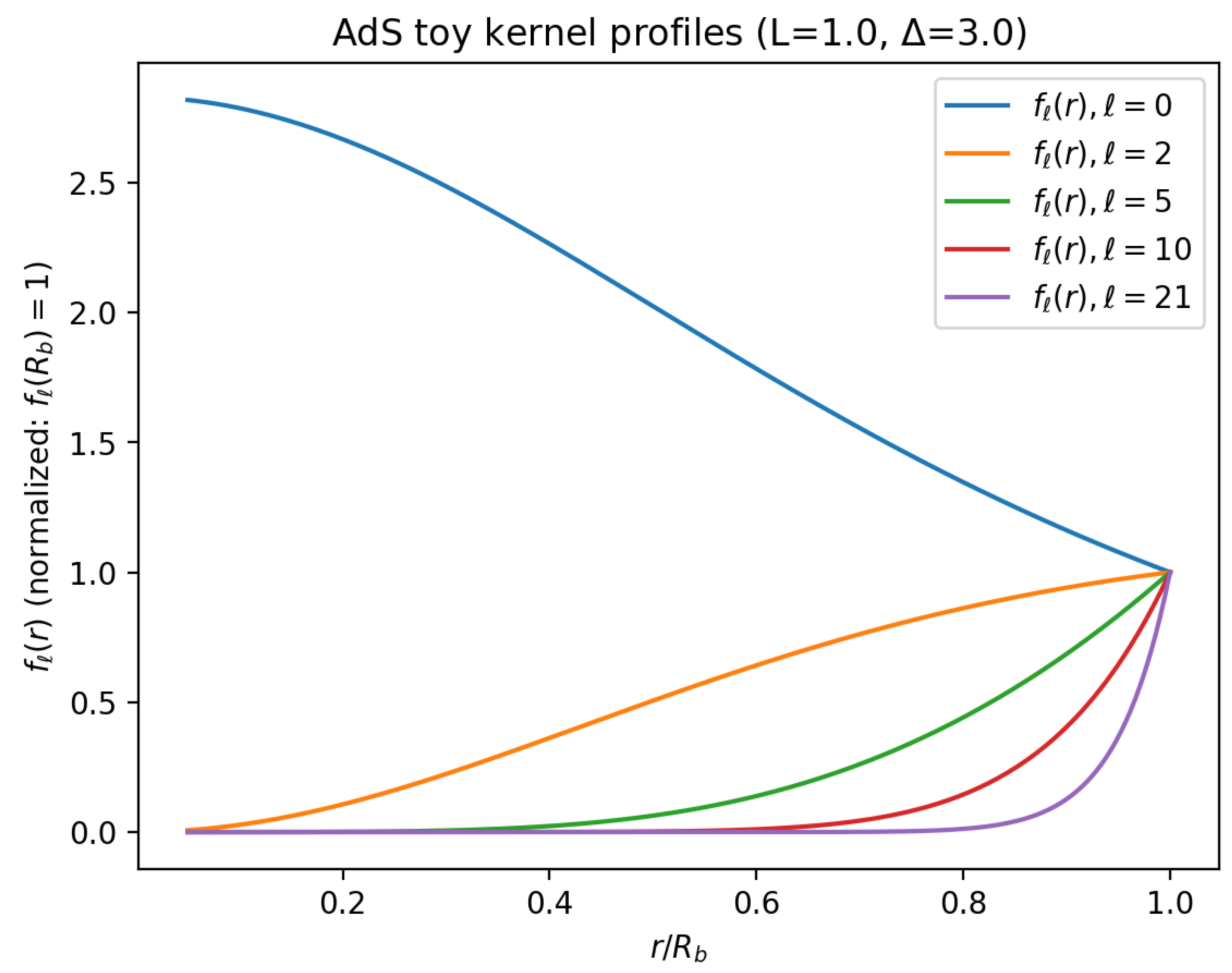
For a clean numerical demonstration we choose a simple, AdS-motivated radial kernel and fix it by the normalization :
Here controls the strength of “conformal damping”; in our runs we use , consistent with the effective scaling for a massless scalar in AdS4 [23,24]. Importantly, the goal here is not to implement the exact hypergeometric radial solutions of the full AdS wave equation, but to validate the HBMB cutoff logic and to compare the structure to HKLL. The kernel can later be replaced by an exact without changing the capacity-controlled angular argument.
Figure 31.
Typical profiles of the chosen AdS toy kernel for several ℓ values (normalized to ). The kernel transports angular modes into the bulk with an ℓ-dependent radial weighting.
Figure 31.
Typical profiles of the chosen AdS toy kernel for several ℓ values (normalized to ). The kernel transports angular modes into the bulk with an ℓ-dependent radial weighting.
7.3. HBMB Cutoff (Capacity) and the Role of the Toy
The number of spherical-harmonic modes up to a cutoff is
At the toy level we identify this with an effective bit-capacity parameter:
Remark:
in the toy sections is a dimensionless effective capacity parameter chosen so that the HBMB cutoff lies in a numerically manageable range; for physical horizons one has , hence naturally enormous values arise.
In our runs , so
7.4. Projection and Bulk-Slice Reconstruction
Let denote the boundary/screen target field. The mode coefficients are obtained by projection:
and the bulk-slice reconstruction at is
Numerically, we implement the projection in a FAST manner (FFT in and Gauss–Legendre quadrature in ).
7.5. Error Metrics and Spectral Coverage
We evaluate the relative error on the bulk slice:
where denotes the “ground-truth” bulk slice (constructed with a sufficiently large reference cutoff) under the same kernel.
We quantify spectral coverage via a Parseval-type energy ratio [20]:
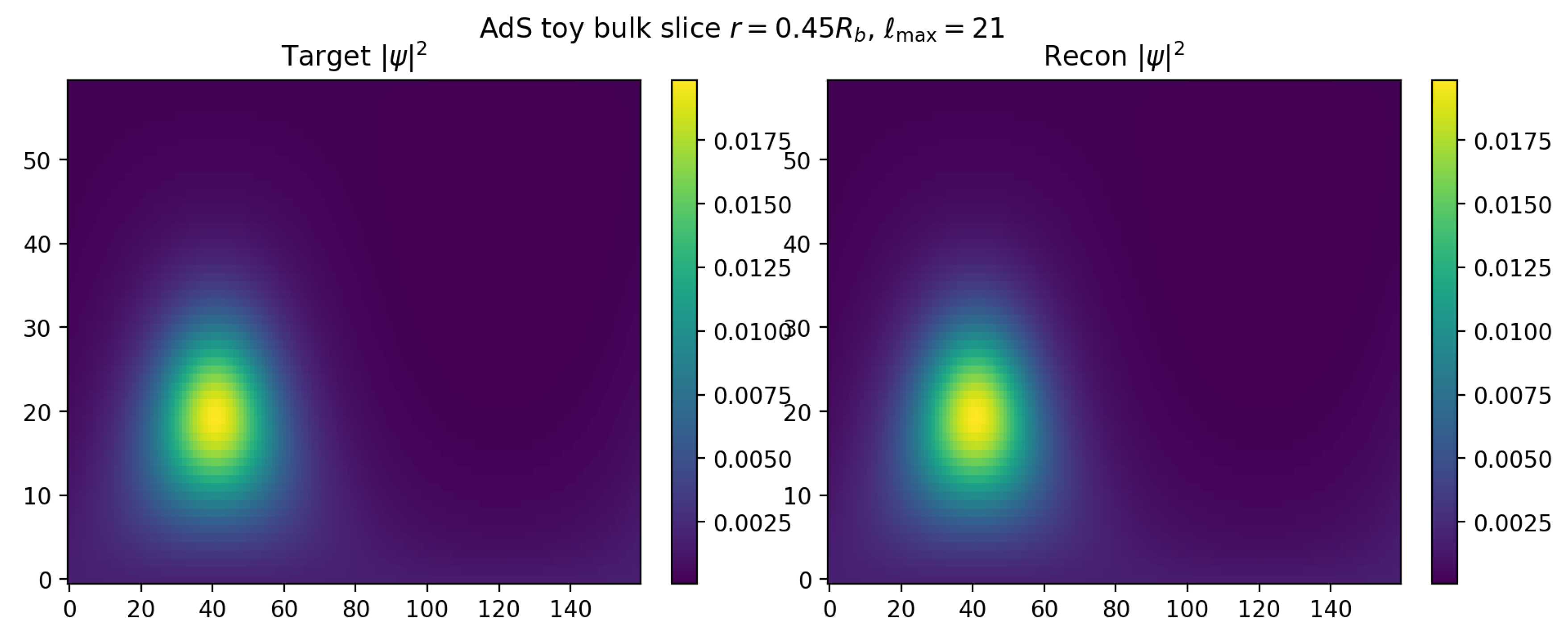
7.6. Numerical Results: AdS Toy “Blob” Target on a Bulk Slice
In the main demonstration, the boundary target is a smooth localized “blob” on the sphere (the same target class as in the flat/dS toy sections), and we reconstruct the bulk slice at using (82).
The error curve and coverage show that convergence is again controlled by the angular cutoff:
while
This is consistent with the intuition that the radial kernel primarily transports and reweights modes in the bulk, while the number of independent angular degrees of freedom is still set by the capacity-limited .
Figure 32.
AdS toy: bulk-slice reconstruction error versus .
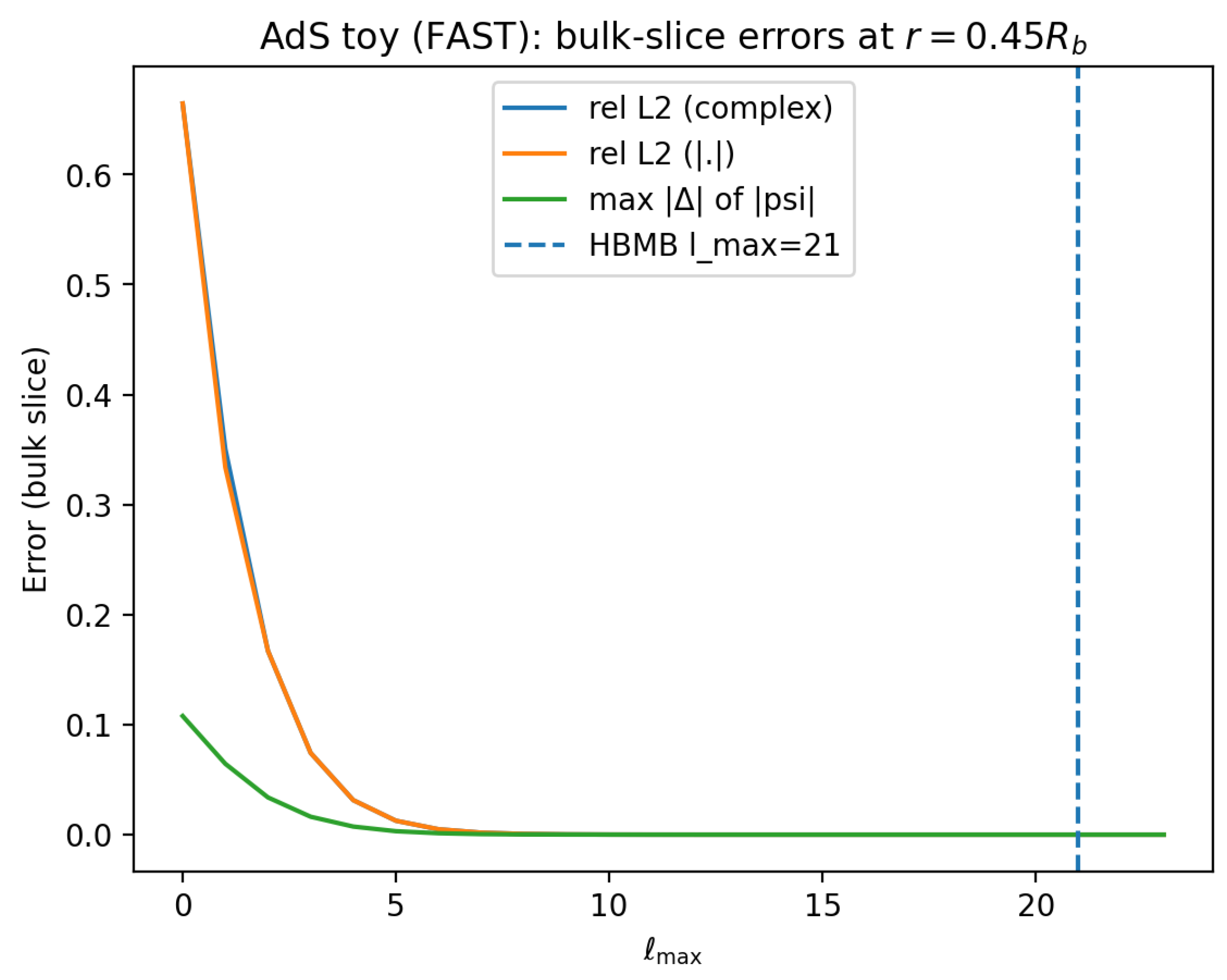
Figure 33.
AdS toy: spectral coverage versus the cutoff.
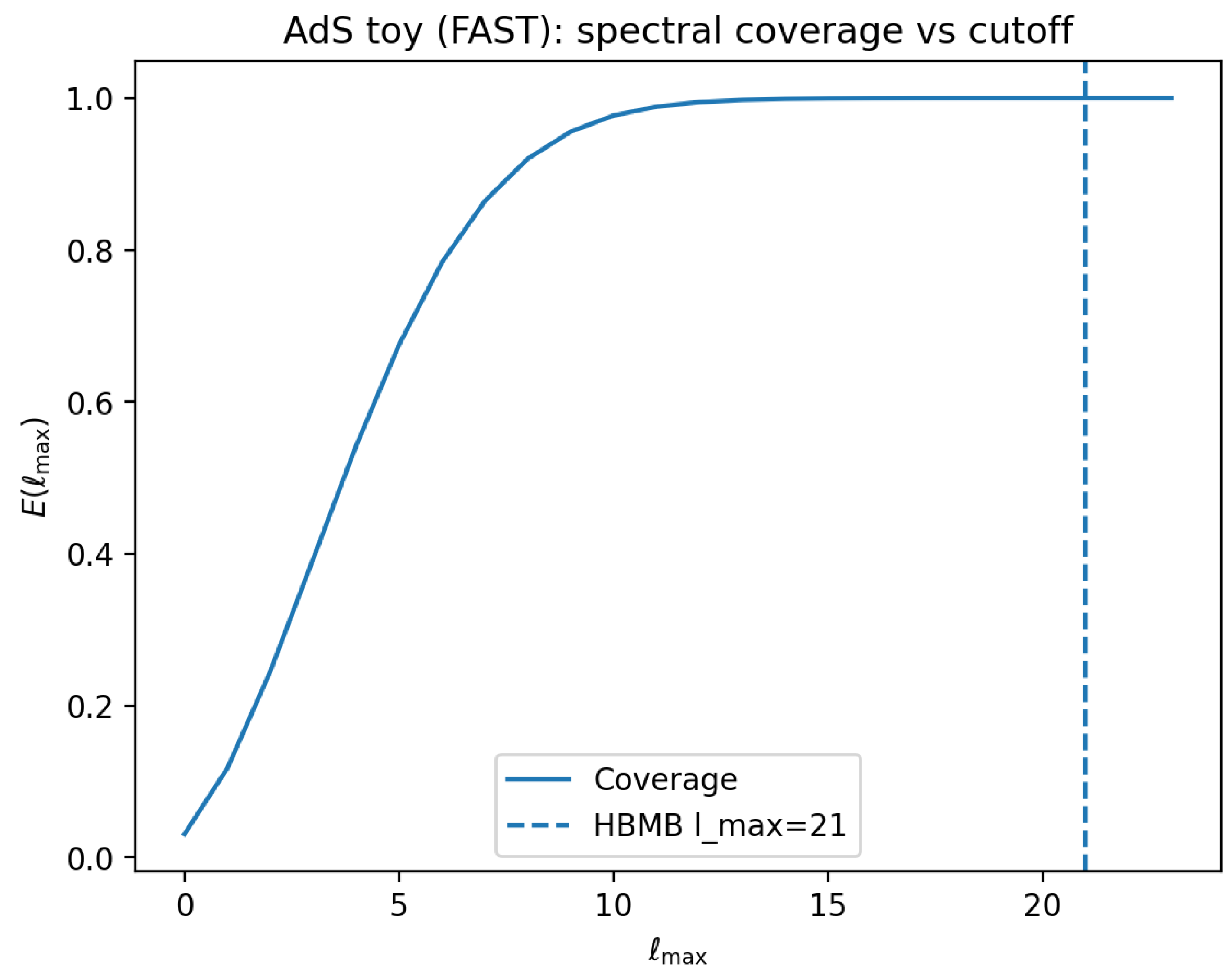
Figure 34.
AdS toy: bulk-slice maps () at .

Figure 35.
AdS toy: bulk-slice maps () at the HBMB cutoff, .
7.7. Control Benchmarks: Hydrogen Target and Complex Superposition (with the AdS Kernel)
The purpose of the angular control tests is to validate the pipeline (projection + truncated synthesis) on analytically controlled targets. For hydrogen-like states, the angular dependence is exactly :
so the boundary/screen target is a finite linear combination of . At the HBMB cutoff we obtain
i.e., effectively floating-point zero: the numerical implementation remains consistent even after introducing the AdS kernel.
Figure 36.
Hydrogen control (AdS): relative error versus .
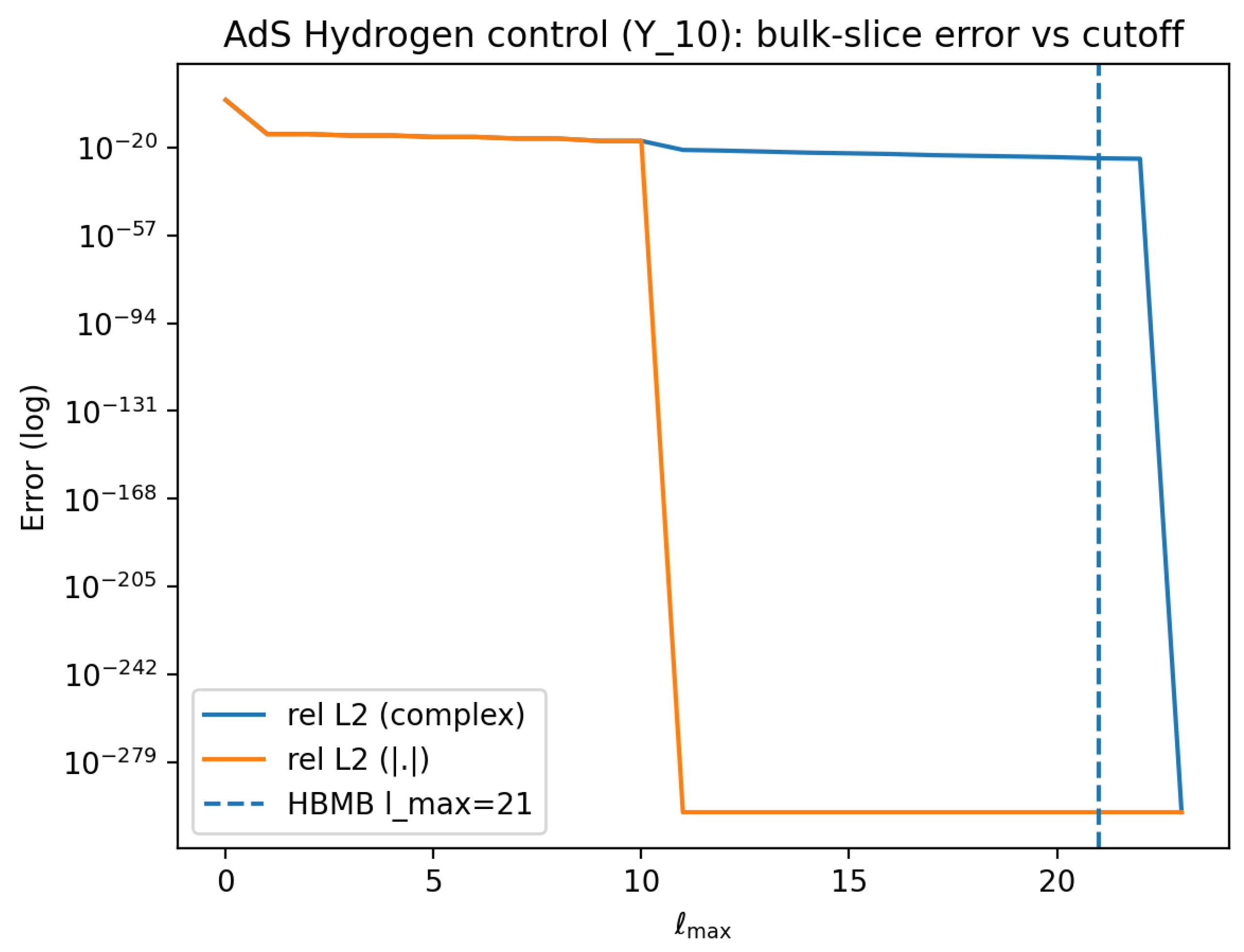
Figure 37.
Hydrogen control (AdS): spectral coverage .
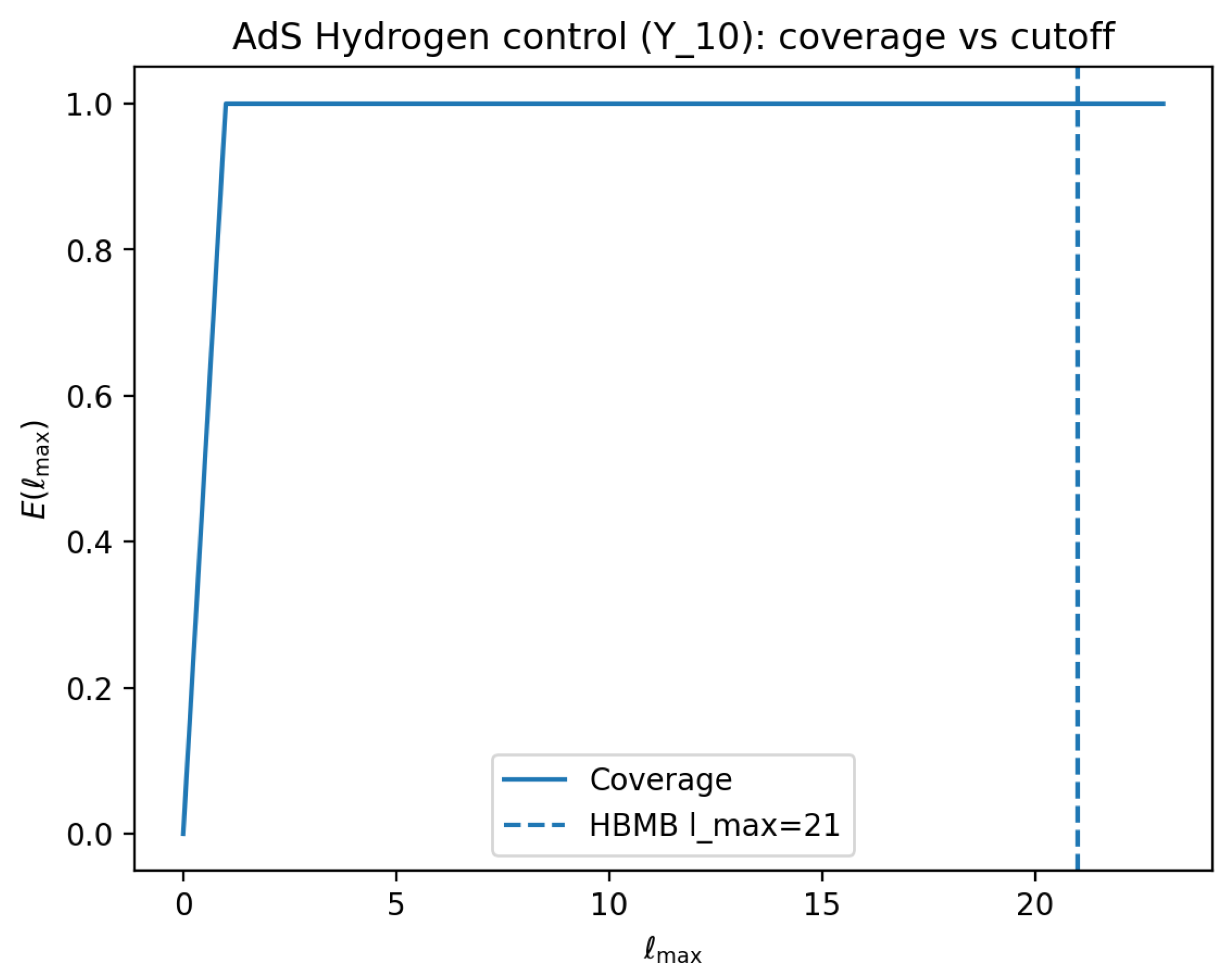
Figure 38.
Hydrogen control (AdS): bulk-slice map at the HBMB cutoff, .
Complex Superposition and Phase Fidelity
We test phase-correct reconstruction with complex-weighted superpositions:
and by linearity,
In our run, the error at closes to numerical zero (machine precision), demonstrating that not only the amplitude but also the complex interference structure is reconstructed correctly.
Figure 39.
Superposition test (AdS): relative error versus .
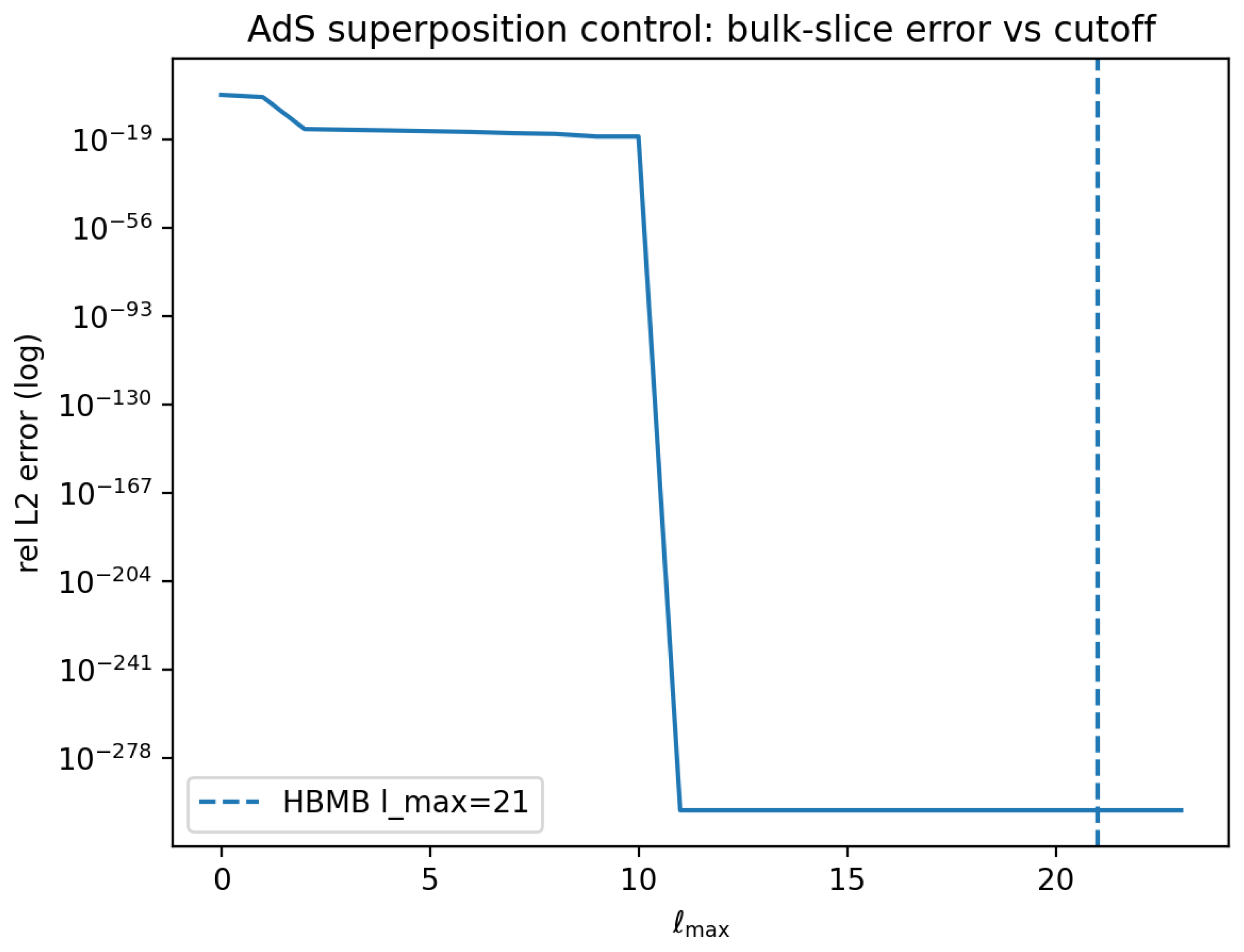
Figure 40.
Superposition test (AdS): phase map at the HBMB cutoff, .
7.8. High-ℓ Stress Test in AdS: A Sharp Cutoff Threshold
In the stress test we choose a boundary target dominated by a critical high-ℓ mode:
The HBMB claim is that reconstruction becomes accurate only once the cutoff reaches the critical mode:
Numerically we obtain the same sharp behavior even with the AdS kernel:
with coverage
Figure 41.
High-ℓ stress test (AdS): reconstruction error versus ; the error collapses once the critical is reached.
Figure 41.
High-ℓ stress test (AdS): reconstruction error versus ; the error collapses once the critical is reached.
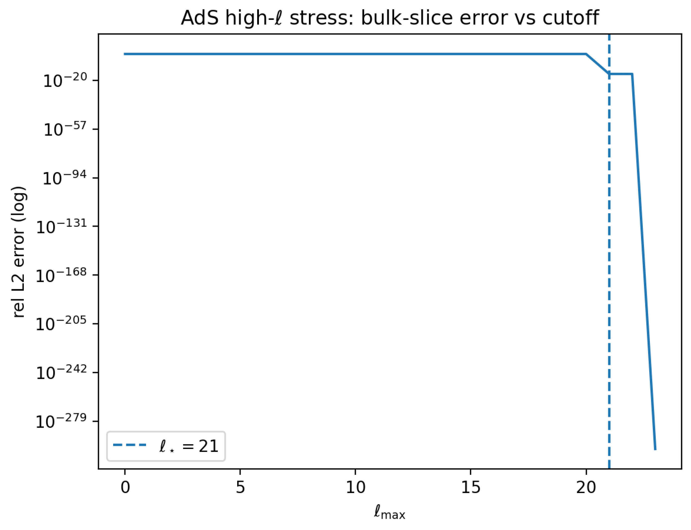
Figure 42.
High-ℓ stress test (AdS): coverage jumps to 1 at the critical cutoff.

Figure 43.
High-ℓ stress test (AdS): bulk-slice map at (the critical mode is still missing).
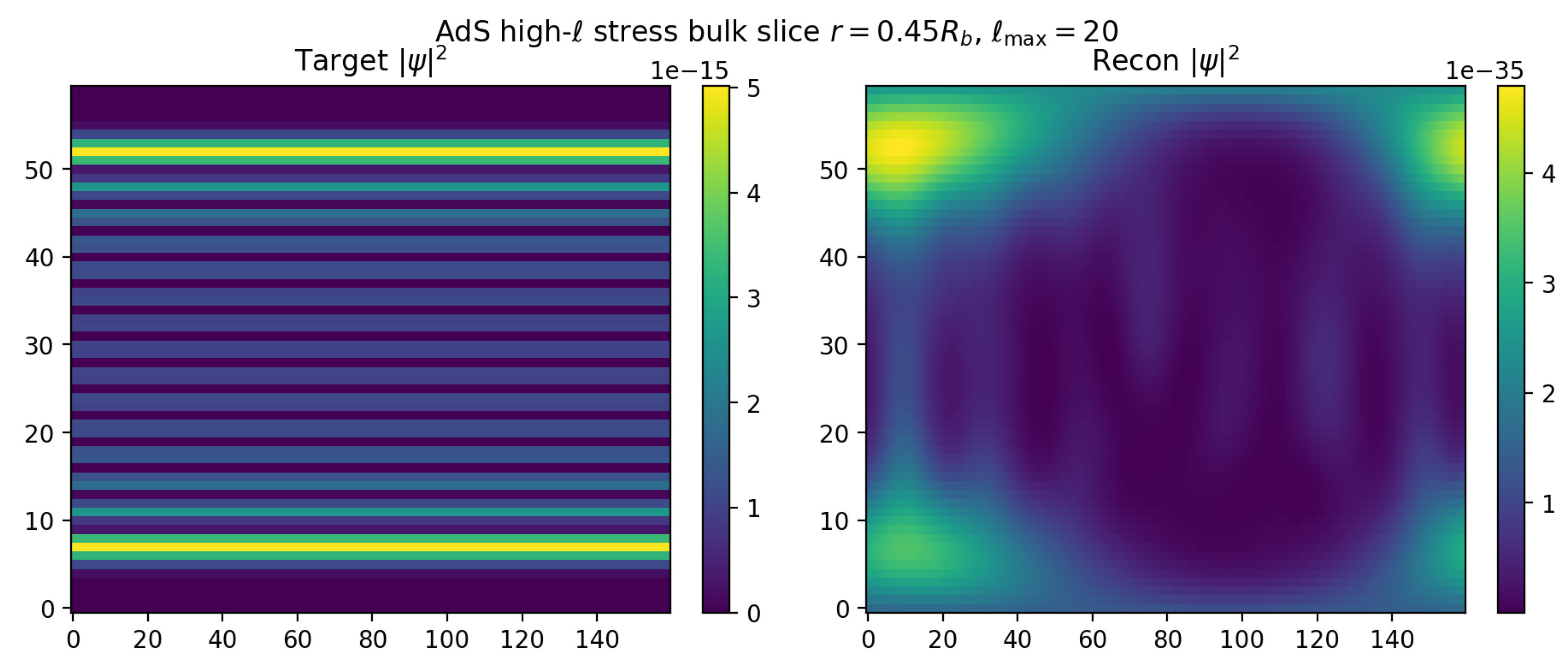
Figure 44.
High-ℓ stress test (AdS): bulk-slice map at (the critical mode is included and the structure appears).
Figure 44.
High-ℓ stress test (AdS): bulk-slice map at (the critical mode is included and the structure appears).
7.9. Literature Comparison: HKLL “Smearing” vs. HBMB Eigensynthesis (AdS)
In the AdS/CFT literature, a standard approach to reconstruct local bulk operators/fields is the HKLL smearing formalism, which builds the bulk quantity from boundary operators using a geometry-dependent kernel [21,22,23,24,25]. In our toy setting we do not study time evolution; the comparison therefore focuses on reconstructing the angular dependence of a fixed bulk slice from boundary/screen data, and on how closely (i) HBMB mode synthesis and (ii) an HKLL-like angular smearing integral agree numerically.
HKLL-Like Angular Smearing
A time-suppressed (purely angular) smearing form is
where is the boundary/screen field on the sphere and is the kernel associated with the bulk slice.
In the spherical-harmonic basis the kernel factorizes mode by mode:
where is the same object as the HBMB “dictionary” radial weight (see the AdS toy-kernel definition). Substituting (96) into (95) and using orthonormality yields
which is exactly the HBMB eigensynthesis form. In this sense, in AdS the HKLL smearing and HBMB reconstruction reduce to the same mode-space structure.
Addition Theorem and a -Dependent Kernel
Direct Numerical Comparison (HKLL Integral vs. HBMB Mode Sum)
We tested the structural equivalence above by computing the bulk-slice field in two ways at the same cutoff :
- 1.
- HBMB: the mode sum ,
- 2.
Comparing the two on sampled points yields agreement at the floating-point limit:
Visually, the amplitude parity plot places the points essentially on the diagonal, and the pointwise amplitude comparison shows the HKLL and HBMB samples lying on top of each other.
Figure 45.
HKLL vs. HBMB amplitude parity plot in AdS. The sampled values of and fall essentially on the diagonal, indicating numerical equivalence within the truncated mode space.
Figure 45.
HKLL vs. HBMB amplitude parity plot in AdS. The sampled values of and fall essentially on the diagonal, indicating numerical equivalence within the truncated mode space.
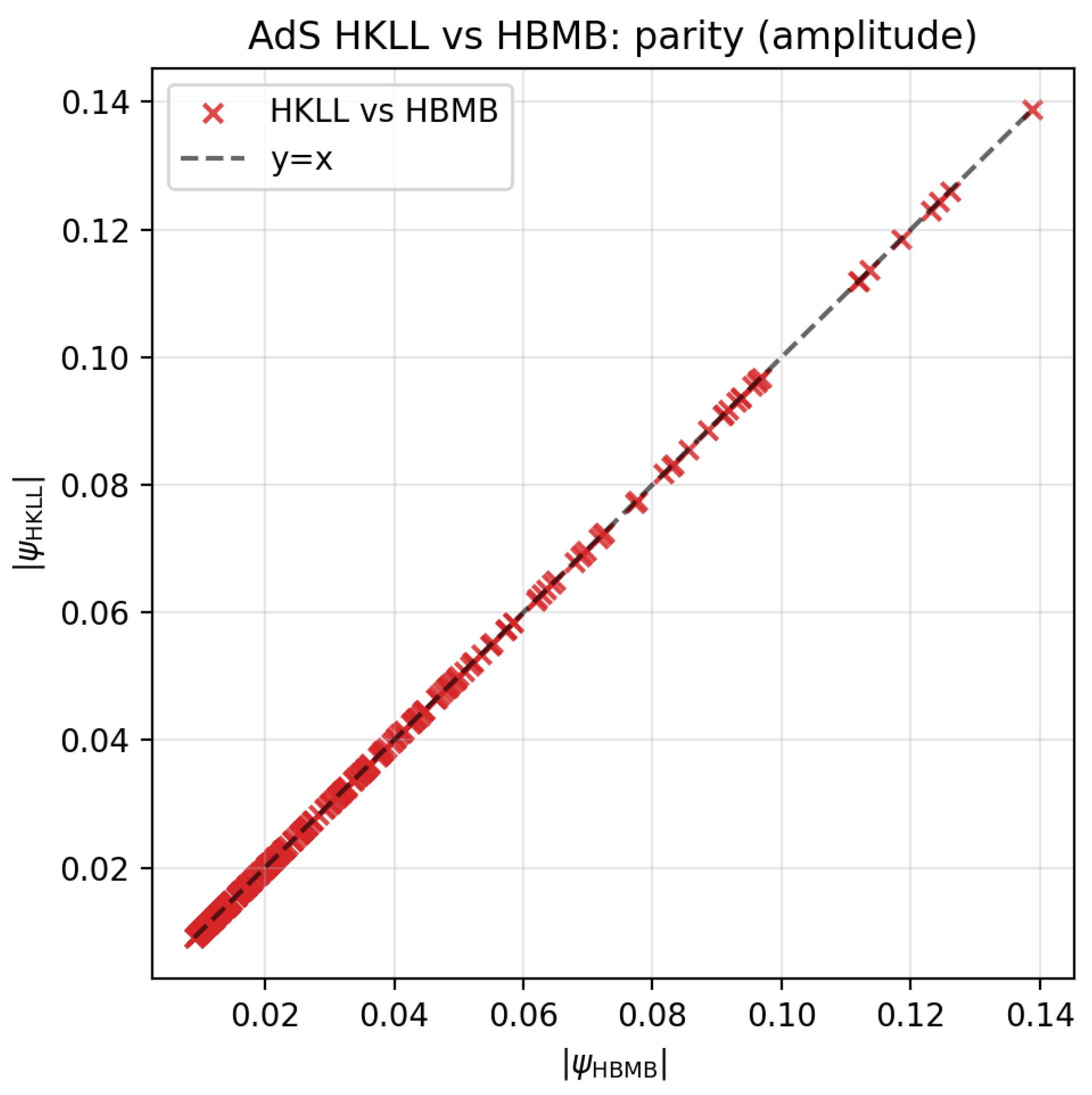
Figure 46.
HKLL vs. HBMB pointwise amplitude comparison in AdS. Blue markers (HBMB) and red x markers (HKLL) overlap on the evaluation points.
Figure 46.
HKLL vs. HBMB pointwise amplitude comparison in AdS. Blue markers (HBMB) and red x markers (HKLL) overlap on the evaluation points.
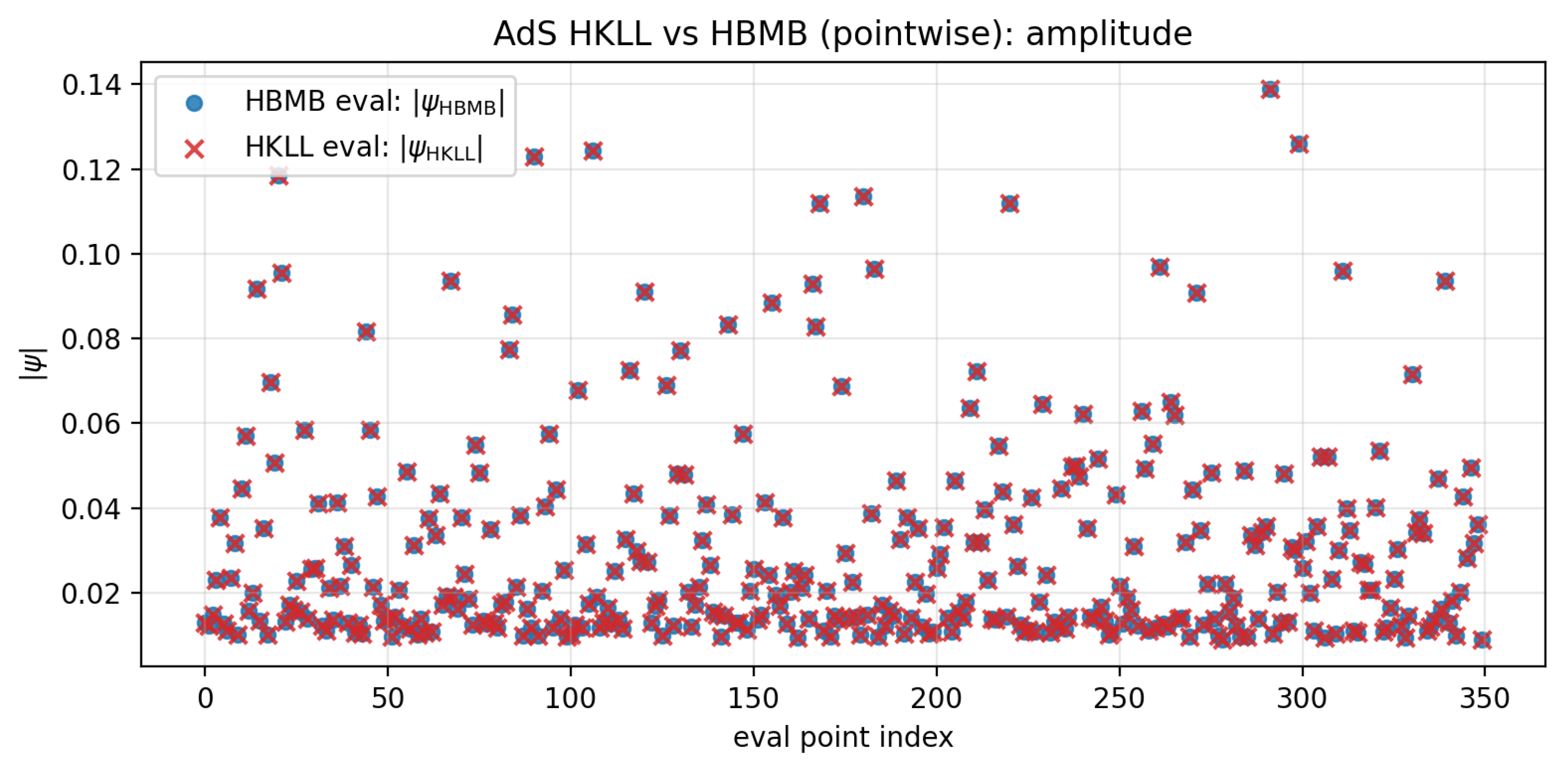
Figure 47.
HKLL vs. HBMB pointwise phase comparison in AdS. The differences are typically at the level, consistent with floating-point rounding and the sensitivity of in regions where is small.
Figure 47.
HKLL vs. HBMB pointwise phase comparison in AdS. The differences are typically at the level, consistent with floating-point rounding and the sensitivity of in regions where is small.
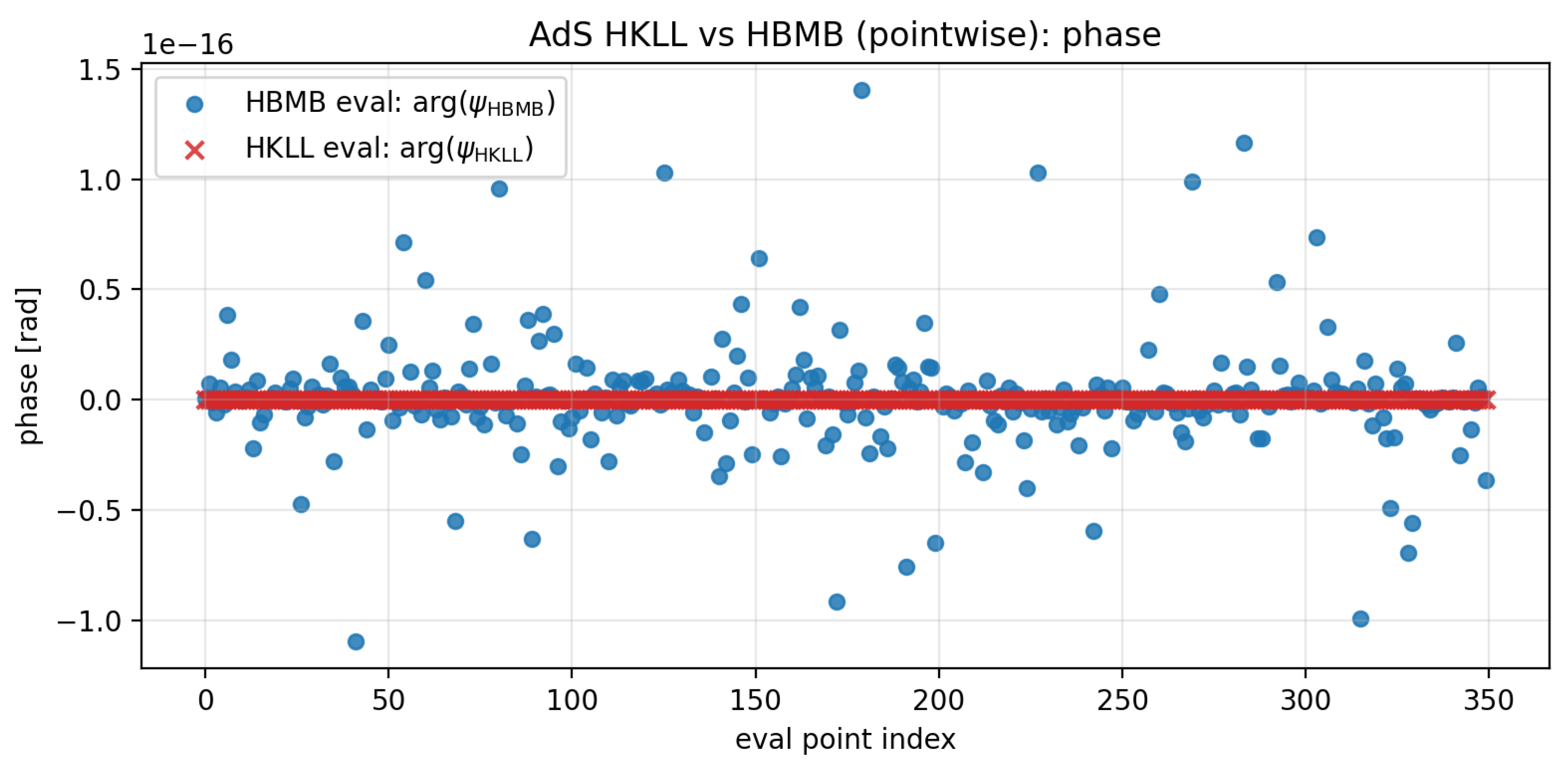
Interpretation and Connection to the Holography Literature
These results are significant in two ways. First, they confirm that the HBMB eigensynthesis used in this chapter realizes the same “boundary → bulk” mathematical structure suggested by HKLL smearing in AdS: reconstruction reduces to mode-by-mode radial weighting. Second, the distinctive physical emphasis of HBMB is not the existence of a kernel, but the fact that reconstruction is constrained by a capacity-derived cutoff ; this yields sharp, falsifiable behavior, as demonstrated by the stress tests above.
7.10. Summary
The main result of the AdS chapter is that the HBMB protocol takes an “literature-compatible” form: bulk reconstruction is naturally expressed in an eigenbasis with an ℓ-dependent radial kernel. The numerical runs show that convergence is again controlled by the angular cutoff, and the high-ℓ stress test produces a sharp capacity threshold in AdS as well. In addition, we directly verified that HBMB mode synthesis and the HKLL-like angular smearing integral (truncated consistently at the same ) agree up to floating-point precision.
8. Nested Horizons as Overlapping Codes
A key element of the HBMB-holographic picture is that the “holographic boundary” need not be a single global object: in physically relevant settings, multiple horizons/screens may appear, nested within each other or partially overlapping (a cosmological horizon in a static patch, a black-hole horizon, the effective Rindler horizon of an accelerated observer, the boundary of a local causal diamond, etc.). Each of these can act as a screen: as a finite-capacity “code” carrying the information required for reconstruction.
This can easily lead to a naive but misleading intuition: if many local screens exist, one might be tempted to add their capacities and conclude that the accessible information can be increased without bound. We refer to this as the overcounting problem. The central claim of this section is that local screens are not independent memories but overlapping, redundant code-views: the same global code state can be encoded by multiple screens in a partially overlapping manner. This viewpoint is also consistent with the modern holographic quantum error-correction (QEC) interpretation, in which the same bulk content can be reconstructed from multiple, partially overlapping boundary subsystems without “duplicating” information [27,28,29].
8.1. Master Horizon Code: Global Code Space and Capacity Bound
Let us consider a master screen/horizon that fixes the global capacity bound of the system under study. The classical Bekenstein–Hawking entropy reads
where is the area of the relevant (global) screen and is the Planck length. We interpret this quantity as a code capacity: physically relevant states live in an effective code subspace,
Local horizons/screens in this picture are not separate Hilbert spaces, but different access-views (reconstruction channels / subalgebras) of the code subspace: multiple “windows” onto the same underlying code space.
8.2. Local Horizons as Overlapping Subcodes: Non-Additive Capacity
Let denote several local screens, each assigned a formal capacity parameter (at toy level, one may take ). Naive overcounting would suggest that the available information is . The correct picture, however, is that the information carried by local screens is redundant: the same code state is encoded in a partially overlapping way. Consequently, the independent (non-redundant) capacity is not additive, and ultimately remains below the master bound:
8.3. Quantitative HBMB Formalism: Overlapping Mode Spaces and Effective Capacity
The natural language of the HBMB protocol is an eigenmode basis together with a truncated reconstruction. Associate to each screen an accessible (truncated) mode subspace ; for a spherical screen, this may be the subspace spanned by modes with . The amount of “independent” information is then not the sum of dimensions, but the dimension of the subspace spanned by the union:
For two screens, the overlap (redundancy) appears explicitly in the basic identity for subspace dimensions:
Hence, the dimension of the intersection directly measures redundancy. For multiple screens, the corresponding inclusion–exclusion structure follows:
which provides an operational (HBMB-compatible) explanation for why the capacity of nested screens is not additive.
8.3.0.7. Remark (Overlap vs. Entanglement)
Operationally, the intersection represents the “common reconstruction domain”: bulk components (modes / operators) that are accessible from both screens. This is not directly identical to a standard entanglement measure (e.g., entanglement entropy), but within the holographic QEC interpretation it is natural that such multiple (partially overlapping) reconstructions arise from redundant encoding enabled by entanglement [27,28,29]. For this reason, the quantity serves as a useful intuition-level analogue of “shared accessibility” (mutual-information-like content), while we remain strictly within the HBMB reconstruction-capacity language.
8.4. Illustrative Figure: Overlapping Code Views (Not a Spacetime Map)
The above logic is illustrated by Figure 48: the master screen fixes a global code-space bound, while local screens define overlapping mode subspaces. The overlap encodes redundancy: the same bulk content may be reconstructible from multiple screens without increasing the independent capacity.
8.5. Connection to Holographic Entropy: Ryu–Takayanagi and Nesting Intuition
In the AdS/CFT literature, the entropy of boundary regions (in the static case) is related to minimal surfaces via the Ryu–Takayanagi formula:
where is the extremal (statistically minimal) surface associated with region A, and is the corresponding bulk region [10,11,26]. For nested/overlapping regions, entanglement-wedge-style nesting intuition suggests that multiple boundary subsystems may provide access to the same bulk content. Our toy “nested horizons” picture is an operational analogue: different screens can encode the same bulk content (at least in a truncated sense) through partially overlapping mode subspaces, and the overlaps naturally lead to a non-additive effective capacity.
8.6. Quantum Error-Correction Viewpoint: ADH and Multiple Reconstructions
In the holographic QEC interpretation, bulk local content is encoded in a code subspace, and certain bulk operators can be reconstructed from multiple boundary subsystems. The Almheiri–Dong–Harlow (ADH) perspective makes this precise by relating bulk locality to error correction [27]; a broader overview is given for example in [28]. Our nested-horizon picture is compatible with this viewpoint: the master fixes the overall code-space bound, while local screens, via the accessible mode subspaces , specify which parts of the code space are reconstructible from which views. Redundancy (overlap) is not a paradox but a signature of robust encoding: the same content can be accessible from several overlapping screens, while the independent capacity does not multiply.
8.7. “Nested Horizon Entropy” as an HBMB-Operational Capacity
Finally, we can introduce a cautious but quantitative definition of an operational capacity for nested screens within the HBMB protocol:
We do not interpret this as a universal entropy law, but as a capacity measure directly tied to HBMB reconstruction: it quantifies the independent (non-redundant) mode content jointly provided by the specified screens. Non-additivity then follows automatically from overlaps, cf. (105)–(106), and it can be interpreted consistently with the master bound (103).
9. Connections to AdS/CFT and QFT
In this chapter we place the HBMB protocol in the context of the holographic and quantum-field-theoretic literature. The goal is not to simply “relabel” HBMB as AdS/CFT, but to (i) make the formal affinity to standard bulk-reconstruction constructions explicit, (ii) record the essential conceptual differences (local screens/horizons and a capacity-driven cutoff), and (iii) provide a minimal and deliberately cautious “wavefunction / code-subspace” interpretation. We emphasize that in HBMB the holographic cutoff is not merely a numerical regularization, but a physically motivated mode-capacity constraint.
9.1. HKLL vs. HBMB Eigensynthesis: Formal Affinity
One of the best-known bulk reconstruction procedures in the holographic literature is the HKLL-type smearing construction [24,25]. Its essence is that a bulk field is reconstructed from boundary operators by a geometry-dependent kernel:
where z is a radial coordinate, x denotes boundary coordinates, is a boundary operator, and is the smearing kernel.
In the HBMB protocol the reconstruction is formally similar (the bulk field is a linear image of boundary/screen data), but the implementation is built from an eigenmode basis: from boundary/screen data we first compute mode coefficients, and then reconstruct the field by a truncated eigenmode synthesis. In a schematic toy form:
where are eigenfunctions (e.g., spherical harmonics), is a radial extension / dictionary factor (geometry dependent), and the coefficients follow from a projection of the screen data,
In HBMB, truncation (e.g., ) is not introduced as a purely technical convenience, but is tied to a physically motivated capacity bound. For a spherical screen, the number of modes
naturally connects to an effective (dimensionless, toy-level) bit-capacity parameter , yielding the HBMB cutoff
9.1.0.8. Summary
HKLL and HBMB share the same overarching structure: a bulk field is obtained from boundary/screen data by a linear map. The difference lies in representation and interpretation: HKLL uses an explicit smearing kernel, while in HBMB the “kernel content” is encoded in the eigenmode expansion together with a geometry-dependent dictionary factor. The numerical AdS comparison presented in the AdS toy chapter (amplitude parity and pointwise phase diagnostics) supports that, for suitable choices, the two procedures can yield near-identical reconstructions, providing a strong consistency check of the HBMB pipeline [24,25].
9.2. Key Differences: Local Screens Instead of a Global Boundary; BH Cutoff; dS Compatibility
We highlight three core differences between HBMB and the standard AdS/CFT setting.
(i) Local screens/horizons, not necessarily a global boundary.
In the classical AdS/CFT formulation the boundary is a global, asymptotic object [21,22,23]. In HBMB, the reconstruction starting point may be a local horizon/screen (a dS static-patch horizon, the boundary of a local causal diamond, an effective horizon for an accelerated observer, etc.). This has an operational advantage: the protocol does not require access to global boundary data of the entire system; in principle, a truncated reconstruction can be built from local physical screen data.
(ii) Capacity-driven cutoff as a physically motivated truncation.
In many standard computations, mode truncation is introduced as a technical regularization. In HBMB, truncation follows from the information-storage capacity of the screen (bit/mode balance): reconstruction can only be consistent up to the mode count allowed by the screen capacity. High-ℓ stress tests particularly demonstrate that this logic is “sharp”: if the critical content of the target field sits in a cutoff-near mode, the reconstruction quality improves dramatically only once the truncation reaches the critical ℓ.
(iii) dS compatibility, AdS/CFT-independence at toy level.
The HBMB toy reconstruction works on a dS static-patch horizon as well, where a global AdS-boundary intuition is not available. The minimum claim here is deliberately cautious: at toy level, an eigenmode-based truncated reconstruction can be performed from local horizon data, and its convergence can be controlled by the capacity-driven cutoff. This suggests that the HBMB protocol is not operationally restricted to an AdS/CFT framework.
9.3. Wavefunction Interpretation and QEC Connection (Cautious)
In HBMB numerical reconstructions we naturally obtain a complex field, which it is convenient to denote as a wavefunction-like object. We distinguish two intentionally different levels of interpretation.
Minimal (Robust) Interpretation
The reconstructed is a complex amplitude field that is consistent with the boundary/screen data within the chosen eigenbasis and the truncated mode space. In this sense, it can be viewed as a “reconstruction state vector” in a truncated Hilbert space. At this level, the method makes no strong assumptions about the fundamental microscopic structure of quantum gravity.
Stronger (Cautious) Interpretation: Code Subspace and Redundant Reconstruction
If screen data can be interpreted at the level of operator algebras, then the truncated mode space can be viewed as an effective code subspace in which bulk information is redundantly encoded. This is consistent with the modern holographic quantum error-correction (QEC) viewpoint, where the same bulk content can be reconstructed from multiple, partially overlapping boundary subsystems without duplicating information [27,28,29]. In HBMB, the capacity-driven cutoff and the language of overlapping screens provide a natural operational bridge to this perspective: reconstruction quality and accessible content are directly tied to the dimension (capacity) of the truncated mode space.
Remark
In this work, by “bulk wavefunction” we primarily mean the complex field reconstructed from boundary/screen data in a capacity-determined truncated eigenmode basis. The emphasis is on operational reconstruction and its cutoff scaling; a microscopic quantum-gravitational identification will be developed in later work (Part II).
10. Scope, Limitations, and Falsifiability
The purpose of this Part I is to introduce and numerically validate an operational holographic protocol: given boundary/screen data, we perform a truncated reconstruction in an eigenmode basis, and demonstrate that reconstruction quality can be controlled by a capacity-determined cutoff. This chapter serves a dual role: (i) it states clearly the minimum claims of the paper (for which we provide explicit numerical evidence), and (ii) it delineates the scope, limitations, and concrete points of falsifiability.
10.1. What We Claim (Toy-Level Demonstrated Results)
(1) Operational reconstruction from local screens.
The HBMB pipeline presented here (screen data → projection onto an eigenbasis → truncated synthesis → error metrics) works across multiple geometries. In the flat and dS cases we use a local spherical screen; in the AdS case we use a local boundary/screen. The protocol is reproducible, numerically stable, and reconstruction error is quantified explicitly.
(2) Capacity-driven cutoff as a reconstruction constraint.
The truncation is not an “aesthetic Fourier trick”: in the high-ℓ stress tests we observe that if the critical content of a target field sits in a given mode , then for the error remains persistently large, while for the reconstruction “opens up” and the error drops by orders of magnitude. This operationally supports the claim that mode capacity is the key limiting resource.
(3) Control benchmarks: machine precision for analytically known eigenmodes.
The hydrogen control runs show that when the eigenbasis of the target field is known and the spectrum fits within the cutoff, the reconstruction reaches machine precision. This validates that the pipeline itself is correct; any remaining error (when present) genuinely originates from truncation/cutoff.
(4) Literature comparison in AdS: parity between HBMB eigensynthesis and HKLL smearing.
In the AdS toy chapter we provide a direct numerical comparison between HBMB reconstruction and an HKLL-like smearing evaluation [24,25]. The observed agreement (amplitude parity and pointwise phase diagnostics) supports that the HBMB protocol is not foreign to standard holographic bulk-reconstruction structures, but rather an eigenmode-language, capacity-cutoff-controlled operational counterpart.
Summary
Together, the points above constitute the “solid core” of the paper: each is backed by numerical data and figures, and multiple independent controls reinforce the conclusions.
10.2. What We Do Not Claim (and Why)
(1) We do not claim a complete, fundamental microscopic theory of quantum gravity.
This paper does not provide an axiomatic micro-description of screen degrees of freedom, does not derive the state space from first principles, and does not derive measurement postulates. The term “bulk wavefunction” is used operationally: the reconstructed complex field is a representation within a truncated mode space (see the remark in the Connections chapter).
(2) We do not claim universality across all geometries and all states.
Our demonstrations are built on toy settings (flat/dS/AdS patches). The goal is to make the protocol logic and the role of the cutoff transparent; full generality (time-dependent backgrounds, strong backreaction, topology changes, etc.) is left to separate work.
(3) We do not derive gravitational dynamics from reconstruction.
In Part I the geometry is taken as a given background at patch level. While the link between capacity and geometry motivates the cutoff, backreaction and emergent Einstein-like dynamics are not part of this paper and naturally belong to the continuation (Part II).
(4) We do not claim direct observational cosmological predictions.
The numerical chapters primarily demonstrate and validate the protocol. Cosmological applications (CMB, structure formation, etc.) are mentioned only as future directions.
10.3. Testable Fingerprints and Falsifiability
A key advantage of the HBMB program is that the method is quantitatively checkable and partly falsifiable already at toy level. Here, falsifiability need not rely on cosmological observations; it can appear as protocol-level tests.
(1) Error scaling with .
Reconstruction error is expected to decrease monotonically as increases, and the spectral coverage should approach unity. If the reconstruction does not robustly exhibit this trend (for the same target field and comparable numerical precision), that indicates either a pipeline issue or an inappropriate choice of basis/kernel form.
(2) Cutoff threshold behavior (high-ℓ stress).
If a target field is constructed to be dominated by a specific mode , then for the reconstruction should fail to reproduce the structure, while for it should appear. If this does not occur, the claim “capacity as the key constraint” is violated.
(3) Cutoff artifacts: aliasing / Gibbs-like boundary effects.
For truncated eigenmode synthesis, sharp or highly localized targets are expected to exhibit truncation artifacts (ringing, overshoot, aliasing-like behavior). These should decrease in a controlled way as increases. If artifact behavior is incompatible with truncation-driven trends, that points to a modeling or implementation issue.
(4) Geometry-dependent yet trend-universal behavior.
Across flat/dS/AdS, details (dictionary factors, patch geometry) differ, but the qualitative behavior of the protocol (error decrease, cutoff role, stress-test threshold) should follow similar patterns. If the protocol systematically breaks down in a given geometry, that identifies a meaningful limitation: either the dictionary/basis choice is not appropriate there, or the minimum HBMB claim is too strong.
Closing Remark
The results of Part I are already checkable: for given screen data, basis, and cutoff, reconstruction quality is quantified with explicit metrics and validated by multiple controls. Part II is not intended to “patch” missing pieces, but to build a microscopic and dynamical interpretation on top of this stable operational foundation.
11. Outlook
This Part I provides an operational, numerically validated building block for the HBMB-holographic program: we demonstrated that a truncated reconstruction in an eigenmode basis from boundary/screen data is stable, reproducible, and that reconstruction quality can be controlled by a capacity-determined cutoff. Across the flat/dS/AdS toy settings and control benchmarks (most notably the high-ℓ stress tests), the results support that the cutoff logic is not merely a numerical regularization, but an operational imprint of the information-storage capacity of the underlying screen. In AdS, the direct comparison to HKLL-like smearing further indicates that HBMB eigensynthesis naturally aligns with standard holographic bulk-reconstruction structures, while the emphasis on local screens extends beyond purely global-boundary intuition.
This paper also connects naturally to the author’s prior HBMB-related works in the sense that the same guiding principle—bit capacity and mode-space balance—is formulated here as a more general, geometry-agnostic reconstruction protocol and supported by explicit numerical evidence. Among the related (stand-alone) companion works, we highlight:
The present Part I, however, is self-contained: it forms a closed, reproducible proof-of-principle unit, and the works listed above are not prerequisites for understanding the reconstruction results reported here.
The continuation (Part II) naturally follows in directions that directly build on Part I; we only list the most immediate, checkable steps:
- Operator-algebraic extension: formalize reconstruction beyond field-level maps, at the level of bulk operators and approximate locality/commutator structure, including a quantitative treatment of nonlocal corrections induced by truncation.
- Dynamic cutoff and backreaction toy models: study minimal settings in which screen capacity and the cutoff evolve with time/scale, and quantify how this feeds back into reconstruction (a step beyond fixed-background toy patches).
- Quantitative QEC connection: deepen the overlapping-screens (overlapping-codes) formalism and connect redundancy/error-tolerance measures to HBMB reconstruction error scaling in an operational manner.
These extensions are not required for the central message of Part I to hold; rather, they provide a natural path to build a microscopic and dynamical interpretation on top of the stable operational foundation established here.
12. Conclusions
In this work (Part I) we formulated and numerically validated a generalized HBMB-holographic principle: starting from boundary/screen data, we reconstructed a bulk field / wavefunction-like complex object operationally via truncated eigenmode synthesis. The central message is that reconstruction is not improved by arbitrary mode refinement in an ad hoc way; rather, convergence and checkability are controlled by a cutoff determined by the information-storage capacity of the underlying screen.
We defined a unified HBMB pipeline and demonstrated it across multiple geometries (flat/dS/AdS patches)—screen data → projection onto an eigenbasis → truncated reconstruction → explicit error metrics—showing that the method is reproducible and numerically stable. Reconstruction error and spectral coverage improve systematically as the cutoff is increased, while the high-ℓ stress tests exhibit a clear threshold behavior: if the critical content of the target field resides in a specific mode , then for the reconstruction is necessarily incomplete, and it becomes accurate only once the cutoff reaches the critical ℓ. The control benchmarks (analytically known eigenmodes) further show that, within the accessible mode range, the pipeline closes at machine precision, cleanly separating truncation-driven information loss from purely numerical limitations.
The AdS toy studies are particularly important for situating HBMB within the existing literature: we provided a direct numerical comparison between HBMB eigensynthesis and HKLL-type smearing reconstruction, and the observed practical parity (amplitude agreement and pointwise phase diagnostics) supports that the HBMB framework naturally aligns with standard holographic bulk-reconstruction structures. In parallel, the nested-horizons chapter clarifies that multiple local horizons/screens do not imply a naively additive capacity; instead, they correspond to overlapping, redundant code views. Intersections of the associated mode spaces operationally quantify redundancy, and the independent (non-redundant) capacity remains consistent with a master bound.
Throughout Part I we used the term “bulk wavefunction” deliberately in an operational sense: it denotes the complex field reconstructed from boundary/screen data in a capacity-determined truncated eigenmode basis. A microscopic quantum-gravitational identification and a dynamical extension are not prerequisites for the numerical results established here, and they form the natural subject of the continuation (Part II). Overall, this paper provides a reproducible, quantitatively checkable proof-of-principle for a generalized HBMB-holographic reconstruction principle: within the mode space limited by screen capacity, a bulk field / wavefunction-like object can be reconstructed consistently, and both convergence and falsifiability can be examined directly through cutoff scaling.
Data Availability Statement
The scripts used to generate the numerical results and figures are available at https://github.com/davenagy86/HBMB_holographic.
References
- J. D. Bekenstein, Black holes and entropy, Phys. Rev. D 7 (1973) 2333–2346.
- S. W. Hawking, Particle creation by black holes, Commun. Math. Phys. 43 (1975) 199–220.
- G. ’t Hooft, Dimensional reduction in quantum gravity, in Salamfestschrift (1993), arXiv:gr-qc/9310026.
- L. Susskind, The world as a hologram, J. Math. Phys. 36 (1995) 6377–6396, arXiv:hep-th/9409089. [CrossRef]
- J. M. Maldacena, The large N limit of superconformal field theories and supergravity, Adv. Theor. Math. Phys. 2 (1998) 231–252, arXiv:hep-th/9711200.
- S. S. Gubser, I. R. Klebanov, A. M. Polyakov, Gauge theory correlators from non-critical string theory, Phys. Lett. B 428 (1998) 105–114, arXiv:hep-th/9802109. [CrossRef]
- E. Witten, Anti de Sitter space and holography, Adv. Theor. Math. Phys. 2 (1998) 253–291, arXiv:hep-th/9802150. [CrossRef]
- T. Banks, M. R. Douglas, G. T. Horowitz, E. Martinec, AdS dynamics from conformal field theory, arXiv:hep-th/9808016.
- A. Hamilton, D. Kabat, G. Lifschytz, D. A. Lowe, Local bulk operators in AdS/CFT: A boundary view of horizons and locality, Phys. Rev. D 73 (2006) 086003, arXiv:hep-th/0506118. [CrossRef]
- S. Ryu, T. Takayanagi, Holographic derivation of entanglement entropy from AdS/CFT, Phys. Rev. Lett. 96 (2006) 181602, arXiv:hep-th/0603001.
- V. E. Hubeny, M. Rangamani, T. Takayanagi, A covariant holographic entanglement entropy proposal, JHEP 07 (2007) 062, arXiv:0705.0016 [hep-th]. [CrossRef]
- A. Almheiri, X. Dong, D. Harlow, Bulk locality and quantum error correction in AdS/CFT, JHEP 04 (2015) 163, arXiv:1411.7041 [hep-th]. [CrossRef]
- D. Harlow, The Ryu–Takayanagi formula from quantum error correction, Commun. Math. Phys. 354 (2017) 865–912, arXiv:1607.03901 [hep-th]. [CrossRef]
- D. Harlow, D. Stanford, Operator Dictionaries and Wave Functions in AdS/CFT and dS/CFT, arXiv:1104.2621 [hep-th] (2011).
- H. Nyquist, Certain topics in telegraph transmission theory, Trans. AIEE 47 (1928) 617–644. [CrossRef]
- C. E. Shannon, Communication in the presence of noise, Proc. IRE 37 (1949) 10–21.
- G. W. Gibbons and S. W. Hawking, Cosmological event horizons, thermodynamics, and particle creation, Phys. Rev. D 15 (1977) 2738–2751.
- W. G. Unruh, Notes on black-hole evaporation, Phys. Rev. D 14 (1976) 870–892. [CrossRef]
- H. B. G. Casimir, On the attraction between two perfectly conducting plates, Proc. K. Ned. Akad. Wet. 51 (1948) 793–795.
- G. B. Arfken, H. J. Weber, F. E. Harris, Mathematical Methods for Physicists, 7th ed., Academic Press (2013).
- J. Maldacena, “The Large N Limit of Superconformal Field Theories and Supergravity,” Adv. Theor. Math. Phys. 2 (1998) 231–252, arXiv:hep-th/9711200.
- S. S. Gubser, I. R. Klebanov, A. M. Polyakov, “Gauge Theory Correlators from Non-Critical String Theory,” Phys. Lett. B 428 (1998) 105–114, arXiv:hep-th/9802109. [CrossRef]
- E. Witten, “Anti de Sitter Space and Holography,” Adv. Theor. Math. Phys. 2 (1998) 253–291, arXiv:hep-th/9802150. [CrossRef]
- A. Hamilton, D. Kabat, G. Lifschytz, D. A. Lowe, “Holographic Representation of Local Bulk Operators,” Phys. Rev. D 74 (2006) 066009, arXiv:hep-th/0606141. [CrossRef]
- A. Hamilton, D. Kabat, G. Lifschytz, D. A. Lowe, “Local Bulk Operators in AdS/CFT: A Boundary View of Horizons and Locality,” Phys. Rev. D 75 (2007) 106001, arXiv:hep-th/0612053. [CrossRef]
- S. Ryu and T. Takayanagi, “Aspects of Holographic Entanglement Entropy,” JHEP 08 (2006) 045, arXiv:hep-th/0605073. [CrossRef]
- A. Almheiri, X. Dong and D. Harlow, “Bulk Locality and Quantum Error Correction in AdS/CFT,” JHEP 04 (2015) 163, arXiv:1411.7041 [hep-th]. [CrossRef]
- D. Harlow, “Jerusalem lectures on black holes and quantum information,” Rev. Mod. Phys. 88 (2016) 015002, arXiv:1409.1231 [hep-th]. [CrossRef]
- F. Pastawski, B. Yoshida, D. Harlow and J. Preskill, “Holographic quantum error-correcting codes: Toy models for the bulk/boundary correspondence,” JHEP 06 (2015) 149, arXiv:1503.06237 [hep-th]. [CrossRef]
- M. A. Nielsen and I. L. Chuang, Quantum Computation and Quantum Information, Cambridge University Press (2000).
- D. Nagy, “A First-Principles Derivation of the Fine-Structure Constant from Holographic Bit–Mode Balance,” OSF Preprints (v2), 2025. https://osf.io/preprints/osf/hw2je.
- D. Nagy, “U(1)-Driven Local Holographic Horizons: Holographic Bit–Mode Balance and the α-Fixpoint,” Preprints.org, manuscript 202511.1803 (2025). url:https://www.preprints.org/manuscript/202511.1803.
- D. Nagy, “Holographic Vacuum Energy from Quantized Horizons,” OSF Preprints (v1), 2025. https://osf.io/preprints/osf/m8t6h.
| 1 | In numerical implementations, one often evaluates boundary data on a nearby surface with . This is a harmless regularization; results are understood in the limit. |
Figure 48.
Schematic diagram of nested horizons as overlapping codes. The large circle denotes the master screen/code space (capacity bound), while the smaller circles are local screens defining overlapping mode subspaces . The overlap (e.g., ) represents redundancy: “shared” bulk content can be reconstructed from multiple screens without additive growth of independent capacity. The diagram is a code-structure schematic, not a literal spacetime-geometric map.
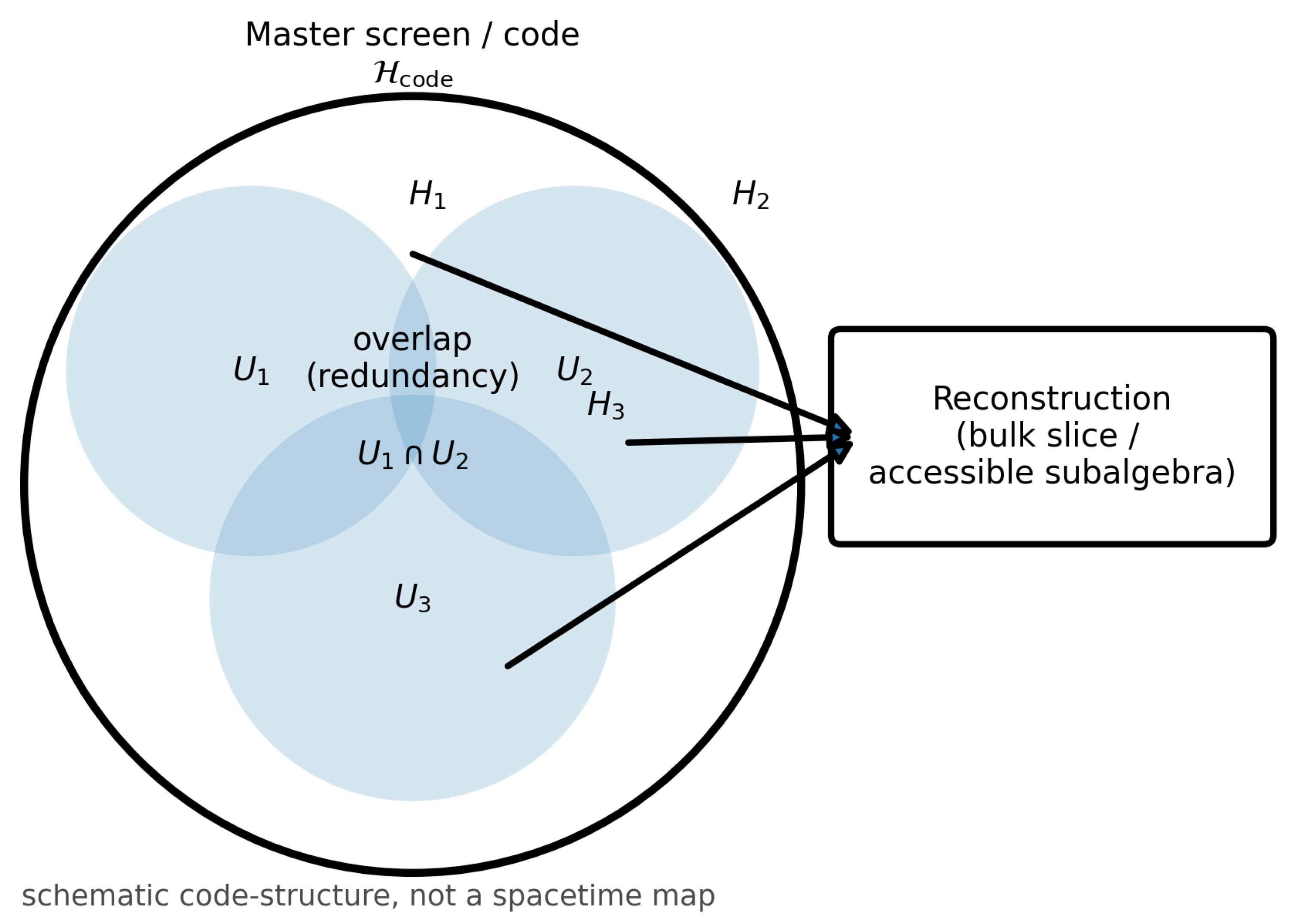
Disclaimer/Publisher’s Note: The statements, opinions and data contained in all publications are solely those of the individual author(s) and contributor(s) and not of MDPI and/or the editor(s). MDPI and/or the editor(s) disclaim responsibility for any injury to people or property resulting from any ideas, methods, instructions or products referred to in the content. |
© 2026 by the author. Licensee MDPI, Basel, Switzerland. This article is an open access article distributed under the terms and conditions of the Creative Commons Attribution (CC BY) license.
Copyright: This open access article is published under a Creative Commons CC BY 4.0 license, which permit the free download, distribution, and reuse, provided that the author and preprint are cited in any reuse.


