Submitted:
16 January 2026
Posted:
19 January 2026
You are already at the latest version
Abstract
Microquasars serve as candidate sites for high-energy particle production within our
Galaxy. Due to their distances, direct observations are relatively limited, necessitating detailed
simulations, in order to connect observations to theory. This work models high-energy particle
emission from relativistic magneto-hydrodynamic microquasar jets. The focus is on neutrino production enhanced by an intermittent jet’s plasmoid collisions with ambient photon fields, found in the surrounding medium. An advanced ray-tracing algorithm processes hydrodynamic simulation data to generate synthetic neutrino images from a stationary observer’s perspective. Synthetic spectra and intensity maps are also produced and can be compared with observations from current and future detectors.
Keywords:
ISM: jets and outflow
; stars: winds–outflows
; stars: flare
; radiation mechanisms: general
; methods: numerical
1. Introduction
Microquasars (MQs) are binary stellar systems comprising a main sequence star orbiting a collapsed stellar remnant [1]. Mass transfer onto the compact object powers relativistic jets launched largely perpendicular to the orbital plane. These jets emit radiation over the electromagnetic spectrum, from radio to very-high-energy (VHE) gamma rays, and also neutrinos [2,3,4,5]. Observations such as apparent superluminal motion support bulk hadronic flows in these jets [2].
Recent ultrahigh-energy (UHE) gamma-ray observations strengthen the case for Galactic compact-object jet systems as potential PeVatron accelerators. In particular, results from LHAASO provide a new UHE view of Galactic gamma-ray sources and motivate renewed interest in jet-powered systems as extreme particle accelerators [6]. Furthermore, UHE gamma-ray emission associated with black-hole jet systems has been discussed in the context of LHAASO detections, providing additional motivation for hadronic acceleration scenarios and associated neutrino production [7]. In parallel, microquasar jet and jet–environment interaction models have recently been explored as PeVatron candidates, including jet–cocoon systems and microquasar remnants as potentially “hidden” PeVatrons [8,9,10].
These developments motivate time-dependent, simulation-based modeling that links RMHD jet dynamics and interaction sites (shocks, plasmoid fronts, terminal regions) to neutrino observables. Since MQ distances and complex geometries limit direct inference, detailed numerical modeling is essential to connect theory with multi-messenger observables.
Strong magnetic fields near jet bases and their tangled structures justify a fluid description via special relativistic magneto-hydrodynamics (RMHD) [11,12,13,14]. Toroidal magnetic components collimate the jet [11,14], while interactions with stellar and disk winds shape jet morphology and confinement [4,15].
Our study combines RMHD jet evolution with neutrino emission modeling, including jet–environment interactions and relativistic effects (beaming, time delays). The focus is on neutrino emission enhancement due to plasmoid collisions with ambient photon and matter fields, with explicit statements of acceleration zones, diffusion regimes, magnetic-field prescription, target photon fields, and the relative roles of and processes.
The paper structure is: Section 2 covers particle acceleration and radiation physics (including explicit zone prescriptions), Section 3 details neutrino emission formalism and target fields, Section 4 describes software tools used, Section 5 provides numerical setup and parameters, Section 6 presents synthetic neutrino results and observability including distance-dependent detectability, and Section 7 summarizes main findings.
2. Theoretical Background
2.1. Particle Acceleration Regions, Mechanisms, and Diffusion Regimes
High-energy protons are accelerated at shock-like structures that naturally arise in intermittent relativistic jets. In the present work we adopt a zone-based description to explicitly specify where acceleration is assumed to occur and what transport regime is used.
Zone A: Internal shocks / plasmoid fronts. Internal shocks form due to velocity irregularities and intermittency; in addition, plasmoid fronts and compressed regions appear due to jet instabilities and jet–wind interactions [3,13]. In the RMHD output, candidate acceleration cells are identified by compression and shock proxies (e.g., negative velocity divergence together with elevated pressure gradients). These regions typically dominate the time-dependent nonthermal power injection.
Zone B: Recollimation / interaction layers. As the jet propagates through ambient stellar and disk winds, recollimation and shear layers can form. These regions can host additional shocks and turbulence, contributing to acceleration and re-acceleration.
Zone C: Terminal / matter-loaded regions (head/cocoon). Toward the terminal regions of the jet where matter accumulates, thermal densities can become high, and hadronic interactions may become significant. This is also where transport may differ from internal plasmoid fronts due to evolving turbulence levels and larger coherence scales.
Acceleration mechanism. We assume first-order Fermi shock acceleration in the above shock-like regions. The acceleration timescale is modeled as
where is an efficiency parameter (order — for relativistic shocks), B is the local magnetic field, and the proton energy.
Diffusion regime and region-dependent transport. Particle transport is controlled by the turbulence level and magnetic-field structure. We adopt an explicit diffusion coefficient parameterization
with chosen by zone to reflect different turbulence regimes. In strongly turbulent, shock-compressed plasmoid fronts (Zone A), we use near-Bohm scaling (), whereas in more quiescent downstream / cocoon regions (Zones B/C) we adopt a weaker energy dependence ( or ). This zone dependence is motivated by recent discussions of microquasar-remnant transport and region-dependent diffusion [10]. The adopted coefficients are used consistently in the emissivity pipeline and clearly stated in the model setup.
2.2. Magnetic Field Prescription in Acceleration Regions
The magnetic field entering the acceleration and interaction rates is taken directly from the RMHD simulation output on a per-cell basis. To make the prescription explicit in acceleration zones, we use the following scheme:
- Primary: RMHD cell field. The local B-vector and magnitude are taken from the PLUTO RMHD solution in each cell.
- Equipartition/turbulent amplification control (acceleration cells). In cells tagged as acceleration sites (Zones A/B), we may enforce or verify that the magnetic energy density satisfieswith a model parameter (typically —1). If the RMHD cell field is below the chosen equipartition fraction in a flagged acceleration cell, we adopt a conservative floor with . This makes the assumed field strength in acceleration regions explicit and reproducible.
At the jet base the initial toroidal field is , and the field evolves self-consistently in the RMHD simulation. The above prescription clarifies how B is interpreted/used in acceleration and emission calculations.
2.3. Nonthermal Proton Distribution
Nonthermal protons are described by a power-law energy distribution,
with spectral index [3]. The normalization factor specifies the fraction of hot protons relative to the thermal background density . Proton energies extend up to GeV.
2.4. Origin of Target Photon Fields
To remove ambiguity regarding the origin of photon fields used in interactions, we explicitly model the target photon field as the sum of physically motivated components:
- Companion star field (dominant in many HMXBs). We model the stellar radiation as a diluted blackbody with temperature and radius . At a distance r from the star, the photon energy density scales as . The photon number density can be written aswhere is the blackbody photon number density per unit energy.
- Accretion disk / corona component (when relevant). We include an additional thermal (or quasi-thermal) disk component with effective temperature and characteristic radius , and optionally a coronal power-law tail if needed for higher-energy targets. In practice, this component can be switched on/off depending on the system class and parameter choice, and an accretions disk’s wind simplified construct is used instead.
- Scattered/wind photon field. A fraction of stellar/disk photons can be scattered in the wind environment, producing a more isotropized target field. We may treat this as a scaled component with .
For plasmoid–wind collisions, the stationary lab-frame photon distribution is Doppler-transformed into the jet comoving frame as described in Section 3.
3. Neutrino Emissivity
3.1. Neutrinos Produced Within the Jet
Neutrino production proceeds via pion production in proton–proton and proton–photon collisions, followed by pion decay. The proton distribution in each computational cell is Lorentz-transformed into the observer frame [16], and steady-state transport equations govern the pion and neutrino spectra [3,4,17,18].
3.2. Neutrino Emissivity from Plasmoid–Wind Collision
To include neutrino emission enhancement from plasmoid collisions with ambient photon fields, the stationary photon distribution in the lab frame is Doppler-transformed into the jet comoving frame:
where is the Doppler factor calculated per cell using local velocity vector and line-of-sight angles, with the velocity reversed to represent incoming photons as seen in the jet frame [20]. The transformed photon distribution replaces the synchrotron photon field used in earlier approaches, and the target field is explicitly decomposed as in Section 2.4.
3.3. Target Photon Distribution and Doppler-Factor Cases Used in Figure 7
For the channel used in our SED calculations, we adopt a power-law target photon distribution in the lab/host frame and implement three prescriptions for the interaction Doppler factor (Cases a–c), as used in Figure 7. The target photon density entering the interaction kernel is written as
Case (a): Constant Doppler factor. A single preset Doppler factor is assumed throughout the emitting plasmoid,
Case (b): Local Doppler factor (cell-based). The Doppler factor is computed locally for each cell using the cell velocity components and LOS angles,
Case (c): Face-on collision approximation. The LOS angles are set to zero (head-on approximation),
In all cases, the velocity vector is reversed in the Doppler-factor evaluation to represent photons entering the jet comoving frame (Appendix A).
3.4. Inclusion of Proton–Proton and Proton–Photon Contributions
Our emission modeling computes neutrino spectra including both proton–proton collisions (expected to be significant in matter-loaded/terminal regions) and proton–photon collisions with ambient photon fields.
Proton–proton pion injection follows
with from [4] and pion distribution as illustrated in Figure 2.
Proton–photon pion injection and neutrino production are computed analogously using the Doppler-transformed photon densities and the relevant cross sections and inelasticities [4]. In Section 6 we provide a direct comparison of the -only, -only, and total neutrino outputs to quantify the role of each channel.
3.5. Velocity and Direction Filtering
To optimize computational costs, cells with velocity vectors aligned close to the observer’s line-of-sight and speeds exceeding are prioritized for neutrino emission calculations. This filtering reduces the number of emitting cells, balancing fidelity and performance. A special “60 points case” restricts emission to a subset of points for benchmarking purposes.
3.6. Main Numerical Emission Expression (Implementation Form)
The explicit numerical form used in the emission code for the neutrino emissivity contribution arising from hadronic interactions (implemented in nemiss) can be written in a numerically convenient triple-integral form. Notation follows that of the main text: is the neutrino energy, the pion energy, the fraction , the fast proton density function, the pion injection kernel (single-collision pion distribution), the inelastic cross-section, and , are implementation-specific normalization/depth factors used in the transport scheme. In the present implementation, the explicit form below corresponds to the contribution; the contribution is computed analogously with the appropriate photon-target interaction kernel (Section and Appendix A).
This algebraic form is the implementation-level emissivity expression used in the code pipeline; it is algebraically equivalent to the standard cascade expression written in terms of and the pion decay kernel after the change of variables and inclusion of transport/depth normalizations. The detailed step-by-step derivation is provided in the Appendix.
4. Computer Programs Used
4.1. Rlos: Relativistic Line of Sight Imaging
The rlos code [21] performs special relativistic imaging by tracing rays through 4D RMHD simulation data, including relativistic beaming and time-delay effects.
4.2. PLUTO Hydrocode
PLUTO [22] is a shock-capturing, finite-volume RMHD code used here for the jet simulations on structured 3D meshes.
4.3. Nemiss
4.4. Additional Tools
Data visualization used Veusz. The codes are publicly available: PLUTO under GPL, nemiss and rlos under LGPL.
5. Model Setup
Our RMHD simulations model intermittent relativistic twin microquasar jets at . The jets propagate into ambient stellar and disk winds, with the companion star located outside the domain [25]. The initial magnetic field is toroidal with strength at the jet base.
Explicit model choices. The acceleration zones are defined as in Section 2.1. We use a zone-dependent diffusion parameterization , adopting near-Bohm scaling () in plasmoid/shock regions and weaker scaling ( or ) in downstream/cocoon regions (see Section 2.1). The magnetic field used in acceleration and interaction rates is taken from the RMHD cell field, with an optional equipartition floor in tagged acceleration cells (Section 2.2). Target photon fields, which may be explicitly decomposed, (Section 2.4) are transformed to the comoving frame where needed; for the SED cases, we additionally adopt the three Doppler prescriptions given in Section 3.3.
The computational mesh is Cartesian cells, each cm in length. Simulation parameters are summarized in Table 1. Neutrino line-of-sight imaging uses local velocity and magnetic field data per cell, with relativistic effects modeled.
6. Results and Discussion
Intermittent twin jets propagate through ambient matter, generating dynamic equatorial structures as jet plasmoids interact with stellar and disk winds (Figure 4).
Synthetic neutrino images at GeV (Figure 5) reveal plasmoid-dominated emission enhanced by velocity filtering.
6.1. Relative Role of and Channels
To quantify the significance of matter targets versus photon targets, we compare the neutrino outputs computed with -only, -only, and combined () emissivities. In matter-loaded and terminal regions, can become competitive or dominant due to increased , while in regions with intense external radiation fields the contribution can be enhanced.
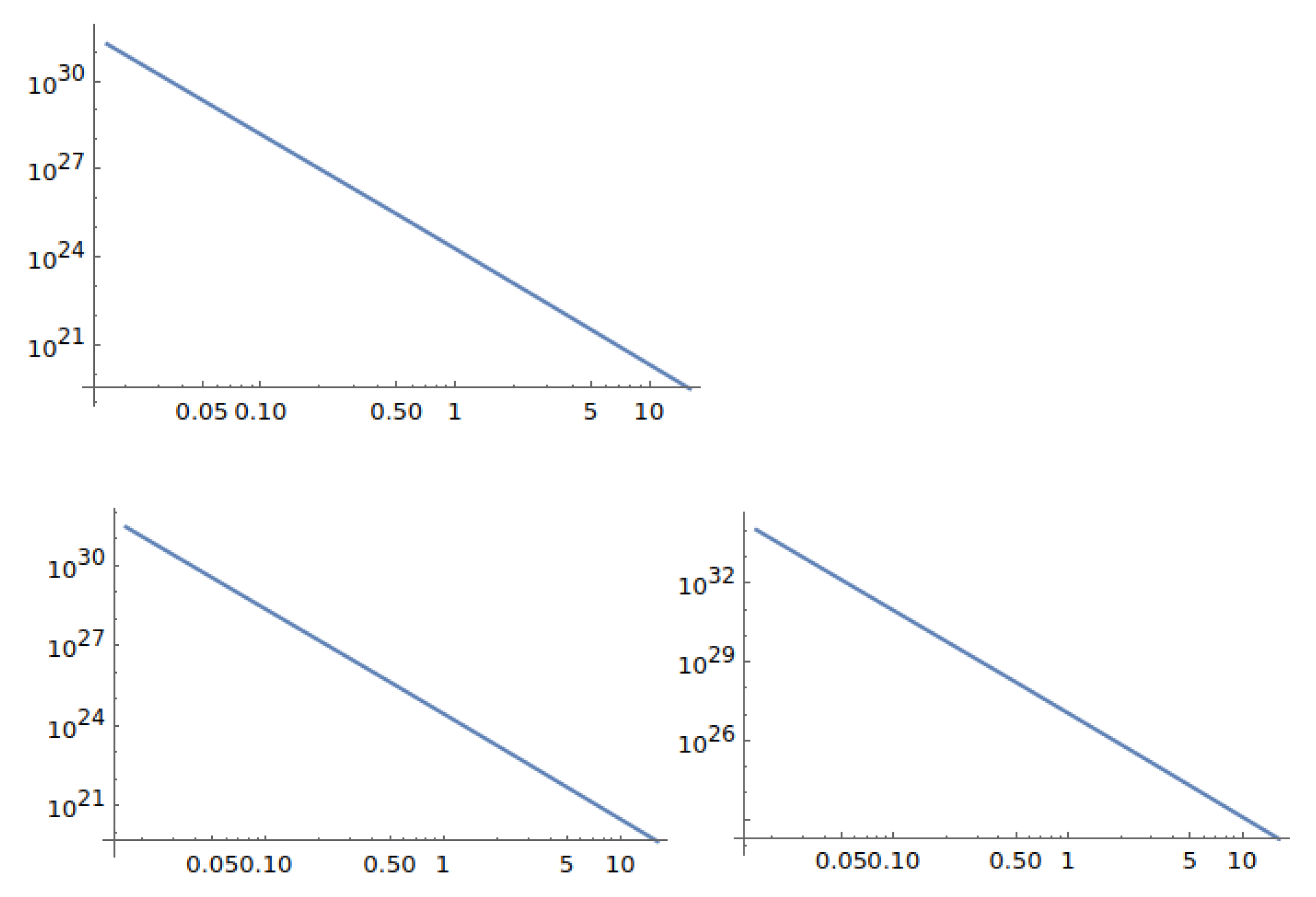
Figure 6.
Comparison of neutrino spectra computed with -only, -only, and total () emissivities at representative snapshots for the three collision scenarios shown in the top, middle, and bottom panels. All three panels are shown in unnormalized (relative) units and are intended solely to illustrate spectral shapes; the absolute normalization is introduced later in Figs. 7 and 10.).
6.2. Flux Normalization, Instrument Sensitivities, and Distance-Dependent Detectability
Figure 7 and Figure 8 present model-based neutrino emission results and their derived detectability. Figure 7 shows the predicted neutrino spectra for different emission prescriptions, while Figure 8 translates these spectra into an energy-dependent distance reach using instrument sensitivities. Figure 10 provides a complementary, instrument-only comparison in detector space, illustrating the relative normalized responses of current and future neutrino observatories across energy, independently of the specific model realization.
To assess detectability, the observable neutrino flux is obtained from the model luminosity via an assumed source distance d. Fluxes scale as
In figures that include observables, we overlay sensitivity curves for relevant instruments (e.g., IceCube, IceCube-Gen2, KM3NeT, Baikal-GVD) and we explicitly state the assumed distance used for flux conversion (here we use a canonical Galactic distance unless otherwise indicated).
A convenient distance-horizon metric at each energy is
where is the instrument sensitivity at energy E. This provides a detectability-versus-distance statement independent of a single assumed distance.
Figure 9 shows the time evolution of total neutrino emissivity at 1.096 GeV.
Relativistic beaming enhances neutrino emission along local flow velocity directions, significantly affecting detectability for microquasars not perfectly aligned with Earth’s line of sight.
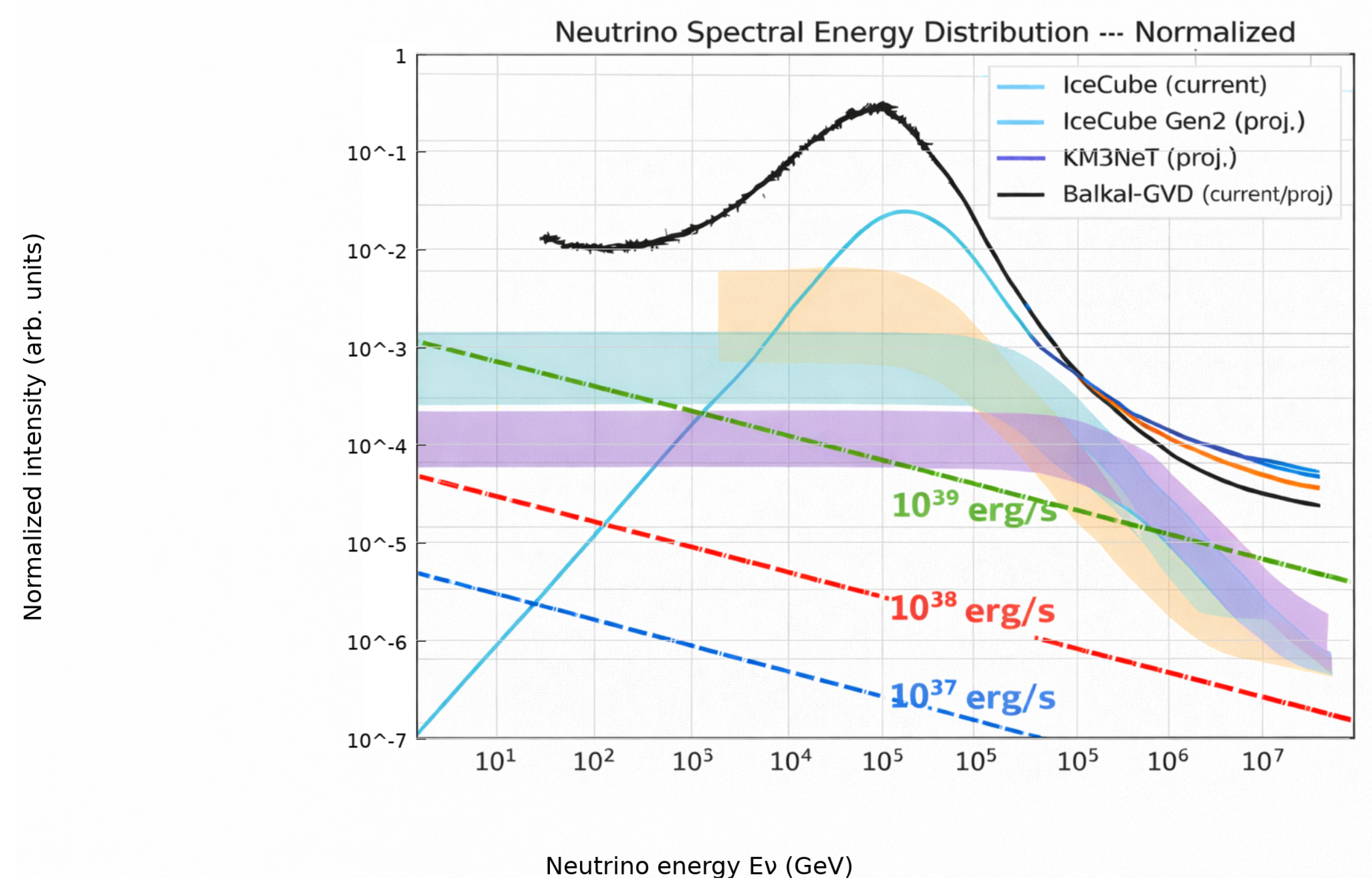
Figure 10.
Normalized neutrino intensity as a function of energy for current and future neutrino telescopes (IceCube, IceCube-Gen2, KM3NeT, and Baikal-GVD). The red curve dashed shows model Case (b), normalized at the source to a total neutrino power (corresponding to of the jet kinetic power), propagated to Earth assuming isotropic emission and mapped onto the normalized-intensity convention used for the experimental sensitivity curves. Shaded bands indicate the typical energy-dependent sensitivity envelopes of each instrument in normalized-intensity space, reflecting variations across analysis channels and effective area.
7. Conclusions
We present a time-resolved model for neutrino emission from relativistic microquasar jets combining RMHD simulations with explicit prescriptions for (i) acceleration zones and mechanisms, (ii) zone-dependent diffusion regimes, (iii) magnetic-field usage in acceleration regions, and (iv) physically motivated target photon fields. Neutrino production includes both proton–proton and proton–photon channels; their relative contributions are quantified, emphasizing that can be significant in matter-loaded/terminal regions.
Synthetic neutrino images and spectra are assessed against the sensitivities of current and upcoming observatories, assuming a canonical Galactic distance and providing a distance-dependent detectability metric. Future work will explore higher resolution, refined radiation-field geometries, and more detailed system-specific parameter sets.
Funding
This research received no external funding.
Institutional Review Board Statement
Not applicable.
Data Availability Statement
Not applicable.
Acknowledgments
The author thanks colleagues for valuable comments on the manuscript. Special thanks go to Professor Gustavo Romero for his insightful comments on an earlier version of this work. The author also gratefully acknowledges important comments from Professor Ralph Spencer.
Conflicts of Interest
The author declares no conflict of interest.
Appendix A. Details on Neutrino Emission and Proton–Photon Interaction Formalism
This appendix outlines the formalism for pion and neutrino production in the jet comoving frame. We summarize the proton–proton () and proton–photon () channels and the Doppler transformation of photon fields into the jet comoving frame.
Appendix A.1. Proton–Proton Interaction and Pion Injection
The inelastic cross section is approximated as [4]:
with and threshold energy GeV.
Appendix A.2. Proton–Photon Interaction Rate
For the proton–photon channel, we use an isotropic photon field in the jet comoving frame. The interaction rate can be written as
where , is the photon energy in the proton rest frame, is the target photon density, is the cross section, and the inelasticity.
Appendix A.3. Doppler Transformations
Quantities computed in the comoving frame are transformed to the observer frame using the Doppler factor
where is the bulk Lorentz factor, , and is the viewing angle.
The angle between the local velocity vector and the line-of-sight unit vector is:
The LOS vector components are:
Photon energies transform as and intensities as appropriate powers of depending on the specific observable discussed in the main text.
Appendix A.4. Line-of-Sight Geometry
The LOS unit vector is parameterized as
The velocity vector is reversed in sign when calculating the Doppler factor for photons incoming into the jet comoving frame.
Appendix A.5. Some Model Setup Details
Appendix B. Full Derivation of Neutrino Emissivity from Proton Interactions
This appendix provides the full derivation of the neutrino emissivity used in the main text. Following [17], the differential neutrino yield from proton–proton interactions is obtained by convolving the proton spectrum with the energy-dependent pion production cross sections and decay kinematics. Explicit expressions for the inelastic cross section, multiplicity, and decay spectra are given here for completeness. Then, proton-photon interactions are described in the formalism.
Appendix B.1. Proton–Proton Channel
We begin with the differential number density of relativistic protons, assumed to follow a power-law distribution in the jet comoving frame,
where is the normalization constant and the spectral index.
The pion injection rate from inelastic proton–proton collisions is
where is the density of thermal target protons and is the pion production spectrum per collision.
Assuming steady state, the pion distribution follows from injection–decay balance,
where is the pion decay timescale.
The neutrino emissivity from charged pion decay is
with . Substituting yields the emissivity integral implemented numerically.
Appendix B.2. Proton–Photon Channel
For the proton–photon channel, the interaction rate in an isotropic photon field is
where , is the photon energy in the proton rest frame, and is the target photon density.
The pion injection rate is then
where is the average inelasticity mapping proton to pion energy.
Following the same steady-state treatment as in the case, the neutrino emissivity is
Appendix B.3. Consistency with Numerical Implementation
Both channels reduce to the same formal structure for neutrino production, differing only in the pion injection term. The expressions above correspond directly to the numerical emissivity kernels implemented in the simulation pipeline and ensure energy conservation and consistency with standard hadronic cascade theory.
Appendix C. Instrumental Sensitivities and Detection Criteria
This appendix summarizes the sensitivity curves and the detection thresholds adopted for the instruments considered in Fig. 10. The plotted curves/bands are taken from the corresponding experimental performance studies and are presented in the normalized units used in the main figure for direct visual comparison.
Appendix D. Normalization of the Model Neutrino Spectrum
Appendix D.1. Source-Level Normalization
The neutrino spectra presented in Fig. 7 are interpreted as differential neutrino power distributions per logarithmic energy interval,
with units of . We assume that a fraction of the jet kinetic power is converted into neutrinos, so that the total neutrino luminosity is
The model spectrum is normalized by enforcing
i.e., the integral over equals the assumed neutrino power.
Appendix D.2. Flux at Earth and Comparison Units
For a source at distance d, the corresponding spectral energy flux is
which preserves the normalization in physical units.
To compare with the normalized-instrument presentation of Fig. 10, we map the model curve into the same plotting scale by applying a single multiplicative factor C (defined in the main text / figure caption) so that
and the resulting curve is overlaid against the instrument sensitivity bands without altering its intrinsic spectral shape.
Appendix D.3. Case Used
Unless otherwise stated, the normalization shown in Fig. 10 corresponds to model case (b) as discussed in the main text.
References
- Mirabel, I.F.; Rodríguez, L.F. 1999, 37, 409.
- Romero, G.E.; Torres, D.F.; Kaufman Bernadó, M.M.; Mirabel, I.F. Hadronic gamma-ray emission from windy microquasars. arXiv 2003, 410, L1–L4, arXiv:astro-ph/astro-ph/0309123. [Google Scholar] [CrossRef]
- Reynoso, M.M.; Romero, G.E.; Christiansen, H.R. Production of gamma rays and neutrinos in the dark jets of the microquasar SS433. MNRAS 2008, 387, 1745–1754. [Google Scholar] [CrossRef]
- Reynoso, M.M.; Romero, G.E. Magnetic field effects on neutrino production in microquasars. A&A 2009, 493, 1–11. [Google Scholar] [CrossRef]
- Reynoso, M.M.; Carulli, A.M. On the possibilities of high-energy neutrino production in the jets of microquasar SS433 in light of new observational data. Astroparticle Physics 2019, 109, 25–32, arXiv:astro-ph.HE/1902.03861. [Google Scholar] [CrossRef]
- Cao, Z.; Aharonian, F.A.; An, Q. The First LHAASO Catalog of Gamma-Ray Sources. Astrophysical Journal Supplement Series 2024, 271. [Google Scholar] [CrossRef]
- LHAASO Collaboration. Ultrahigh-Energy Gamma-Ray Emission Associated with Black Hole Jet Systems. arXiv 2024. arXiv:astro-ph.HE/2410.08988. [Google Scholar]
- Wang, J.; Reville, B.; Aharonian, F.A. Galactic Superaccreting X-Ray Binaries as Super-PeVatron Accelerators. ApJ Letters 2025, 989, L25. [Google Scholar] [CrossRef]
- Zhang, B.T.; Kimura, S.S.; Moors, K. Microquasar jet-cocoon systems as PeVatrons. Physical Review D 2025, 112, 123015. [Google Scholar] [CrossRef]
- Abaroa, L.; Romero, G.E.; Bosch-Ramon, V. Microquasar remnants as hidden PeVatrons. arXiv 2025, arXiv:2512.07781. [Google Scholar] [CrossRef]
- Koessl, D.; Mueller, E.; Hillebrandt, W. Numerical simulations of axially symmetric magnetized jets. I - The influence of equipartition magnetic fields. II - Apparent field structure and theoretical radio maps. III - Collimation of underexpanded jets by magnetic fields. 1990, 229, 378–415.
- Rieger, F.M.; Duffy, P. A Microscopic Analysis of Shear Acceleration. arXiv 2006, 652, 1044–1049, arXiv:astro-ph/astro-ph/0610187. [Google Scholar] [CrossRef]
- Rieger, F.M. An Introduction to Particle Acceleration in Shearing Flows. Galaxies 2019, 7, 78, arXiv:astro-ph.HE/1909.07237. [Google Scholar] [CrossRef]
- Singh2019MHD. Study of relativistic magnetized outflows with relativistic equation of state. Monthly Notices of the Royal Astronomical Society 2019, 488, 5713–5727. Available online: https://academic.oup.com/mnras/article-pdf/488/4/5713/29191239/stz2101.pdf. [CrossRef]
- Hughes, P.A. Beams and Jets in Astrophysics; Hughes, Ed.; Cambridge University Press, 1991. [Google Scholar]
- Torres, D.F.; Reimer, A. Hadronic beam models for quasars and microquasars. arXiv 2011, 528, L2, arXiv:astro-ph.HE/1102.0851. [Google Scholar] [CrossRef]
- Kelner, S.R.; Aharonian, F.A.; Bugayov, V.V. Energy spectra of gamma rays, electrons, and neutrinos produced at proton-proton interactions in the very high energy regime. PhysRevD 2006, 74, 034018. [Google Scholar] [CrossRef]
- Lipari, P.; Lusignoli, M.; Meloni, D. Flavor composition and energy spectrum of astrophysical neutrinos. Physical Review D 2007, 75. [Google Scholar] [CrossRef]
- Smponias, T.; Kosmas, O. Advances in High Energy Physics. 2015, 921757.
- Boettcher, M. Beaming patterns of neutrino emission from photo-pion production in relativistic jets. arXiv 2023, arXiv:2308.01083. [Google Scholar] [CrossRef]
- Smponias, T. RLOS: Time-resolved imaging of model astrophysical jets, 2018, [1811.009].
- Mignone, A.; Bodo, G.; Massaglia, S. PLUTO: A Numerical Code for Computational Astrophysics. Astrophysical Journal Supplement Series 2007, 170, 228–242. [Google Scholar] [CrossRef]
- Smponias, T. nemiss: neutrino imaging of model astrophysical jets,github.com/teoxxx/nemiss_pbl, 2019.
- Smponias, T. Synthetic Neutrino Imaging of a Microquasar. Galaxies 2021, 9, 80. [Google Scholar] [CrossRef]
- Fabrika, S. The jets and supercritical accretion disk in SS433. arXiv 2004, 12, 1–152, arXiv:astro-ph/astro-ph/0603390. [Google Scholar]
Figure 1.
Power-law density of nonthermal protons in the jet, per cm3, without the high-energy cutoff, plotted versus energy.
Figure 1.
Power-law density of nonthermal protons in the jet, per cm3, without the high-energy cutoff, plotted versus energy.
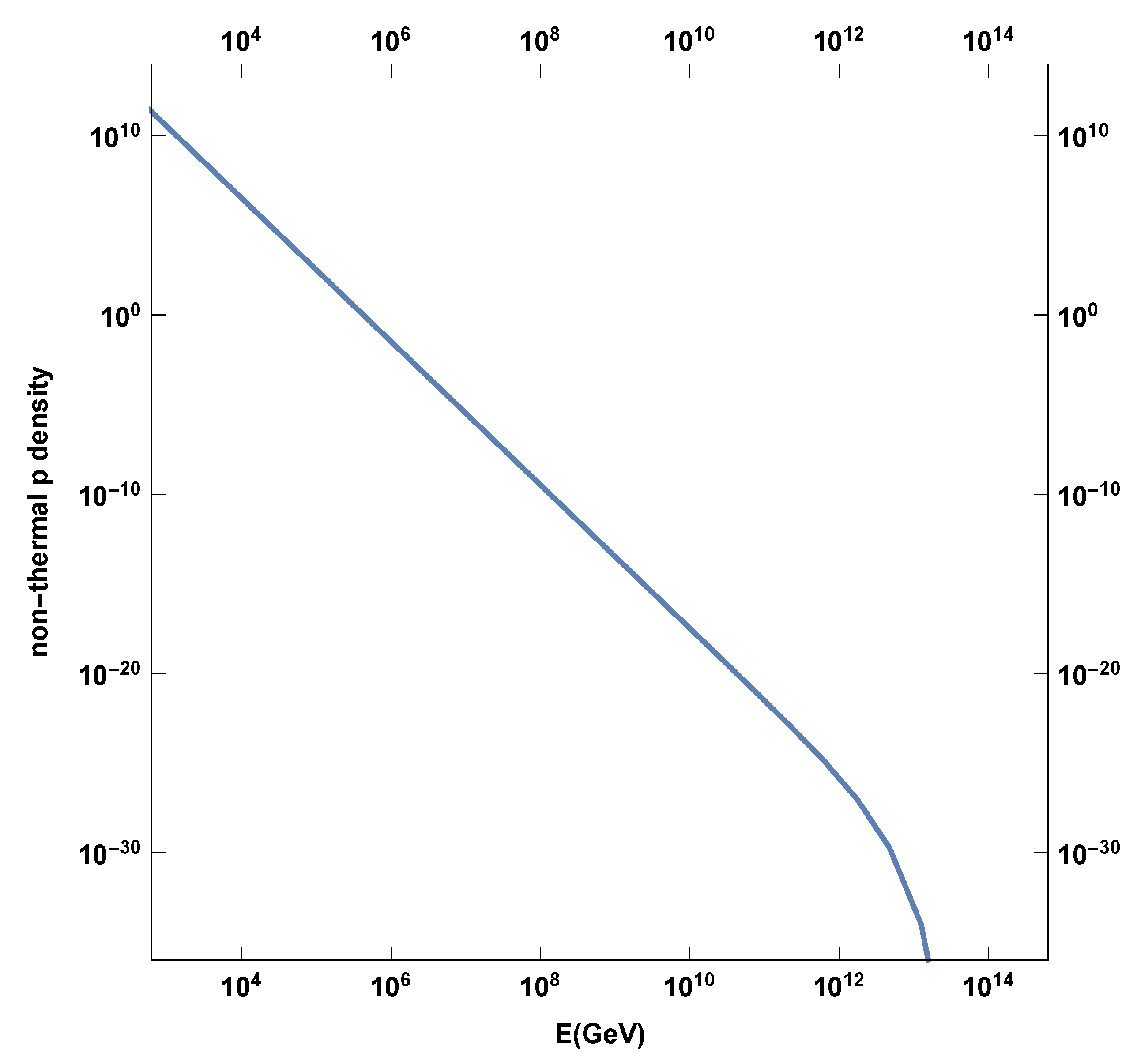
Figure 2.
Pion energy distribution function , plotted versus x=, from single proton–proton collisions at three proton energies.
Figure 2.
Pion energy distribution function , plotted versus x=, from single proton–proton collisions at three proton energies.
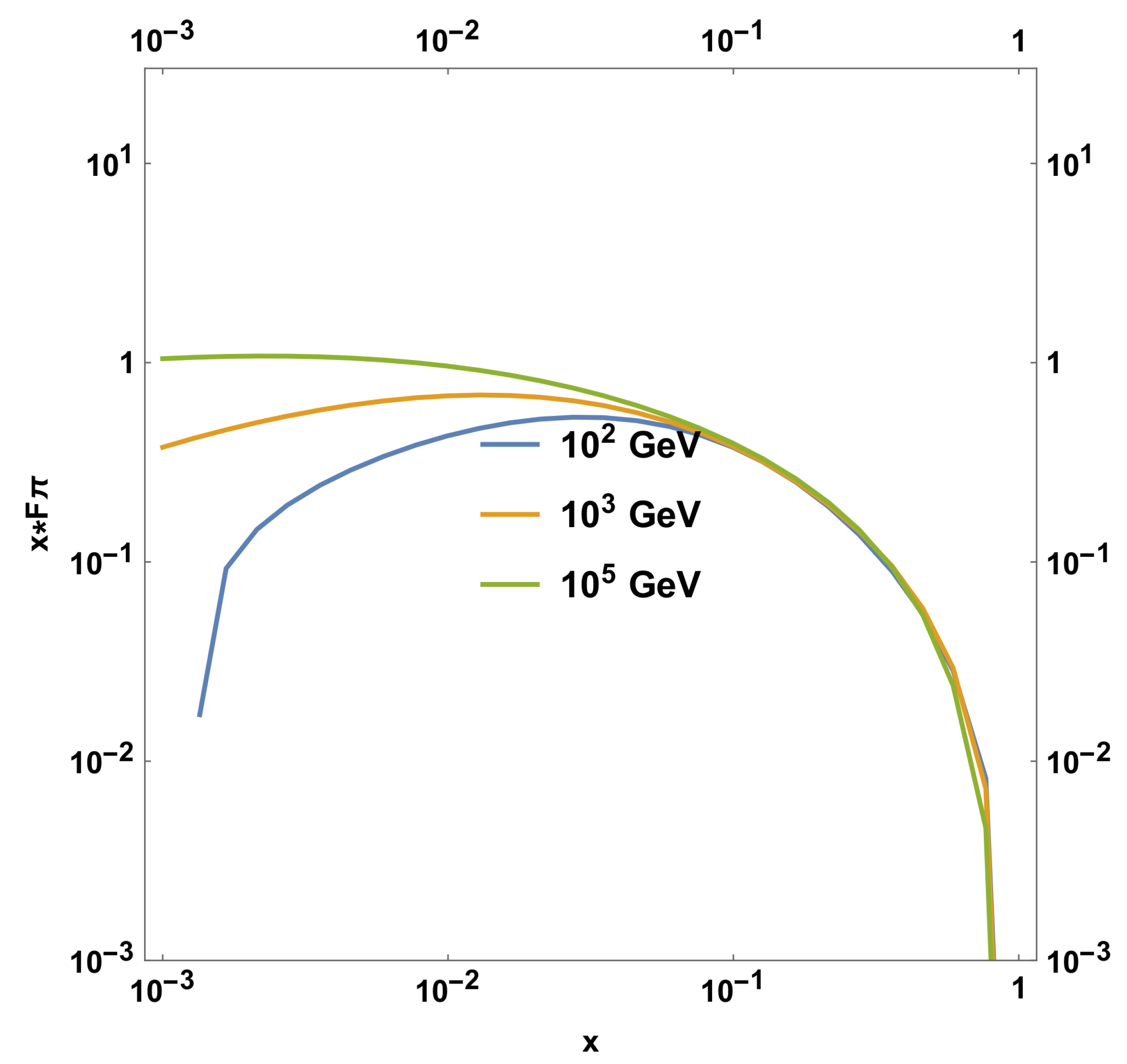
Figure 3.
Pion injection function , from multiple proton–proton collisions, showing an energy-dependent spectrum with a high-energy cutoff.
Figure 3.
Pion injection function , from multiple proton–proton collisions, showing an energy-dependent spectrum with a high-energy cutoff.
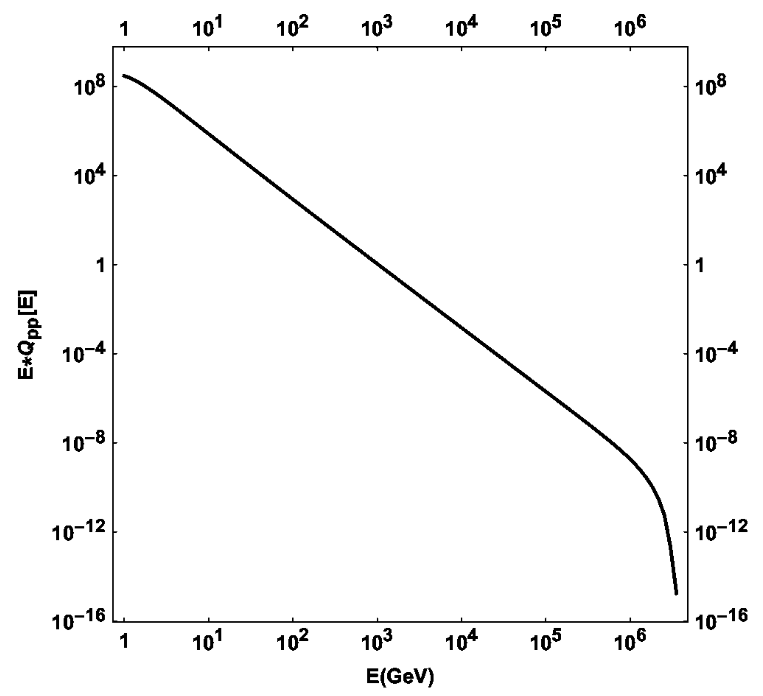
Figure 4.
PLUTO RMHD 3D density rendering of intermittent twin jet plasmoids interacting with stellar and disk winds, producing dynamic equatorial structures.
Figure 4.
PLUTO RMHD 3D density rendering of intermittent twin jet plasmoids interacting with stellar and disk winds, producing dynamic equatorial structures.
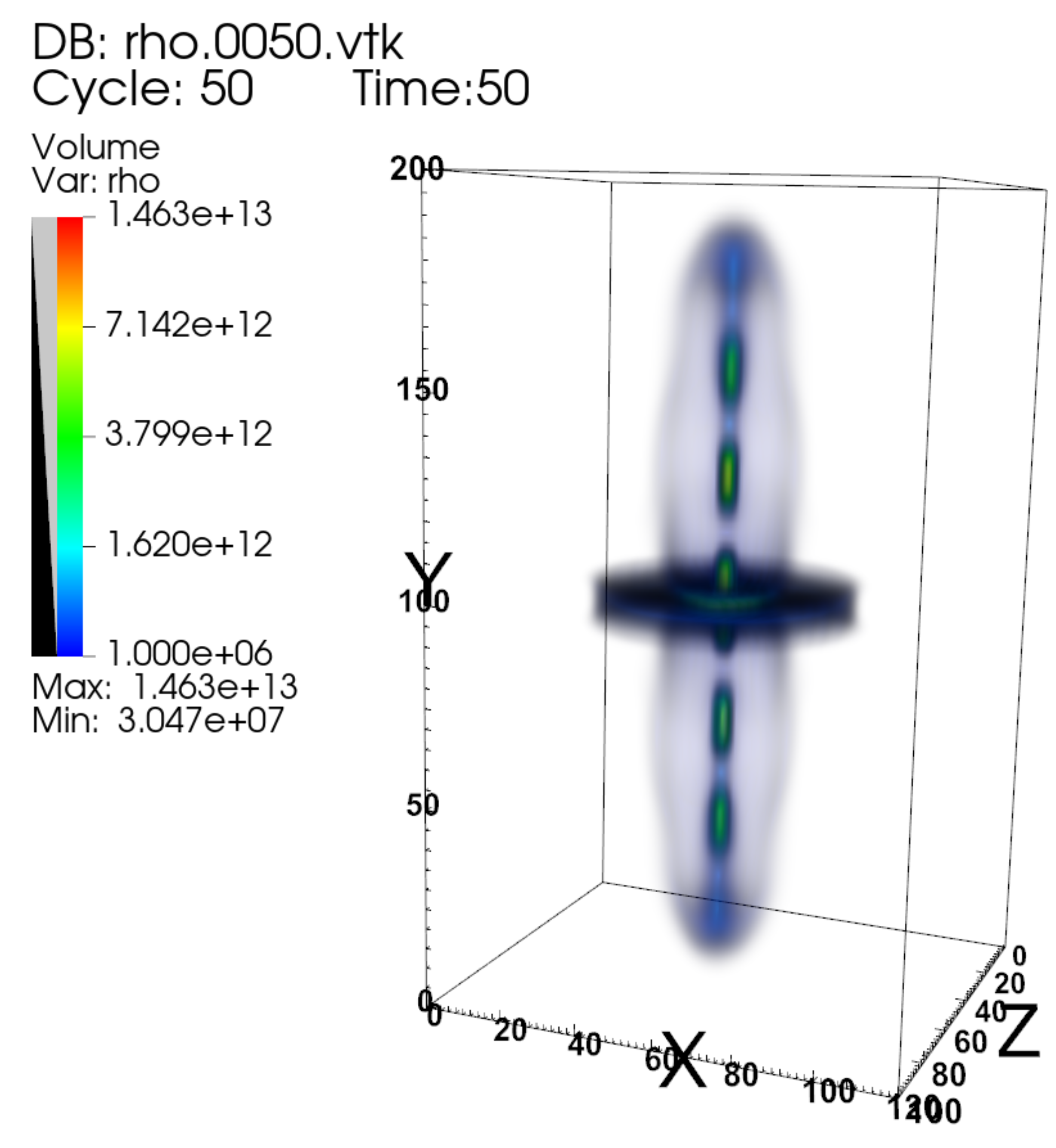
Figure 5.
Synthetic neutrino image at model time 30 s and energy GeV. Velocity and direction filtering highlight plasmoid emission and side beaming.
Figure 5.
Synthetic neutrino image at model time 30 s and energy GeV. Velocity and direction filtering highlight plasmoid emission and side beaming.
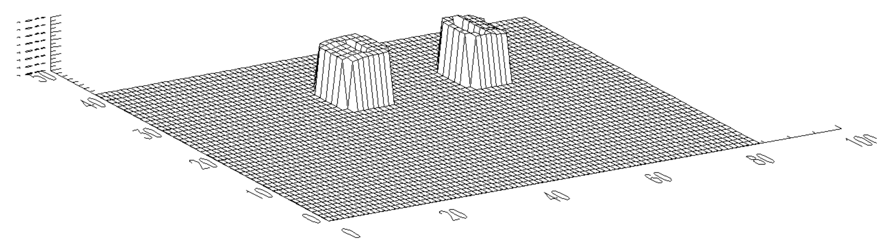
Figure 7.
Neutrino spectra for the different emission cases considered, shown in physical flux units (i.e. expressed in GeV cm−2 s−1). Cases (a)–(c) correspond to spectra obtained from combined and interactions under different collision and emission conditions. Case (d) represents a baseline -only model, computed using a reduced set of representative collision points, and is shown for comparison with the more densely sampled cases. s−1) assuming a source distance of kpc. The curves correspond to the three Doppler prescriptions for the target photon field used in the channel (Case (a), Case (b), Case (c); see Section 3.3) and the total combined emission including both and contributions. Sensitivity curves for IceCube, IceCube-Gen2, KM3NeT, and Baikal-GVD are overlaid for reference.
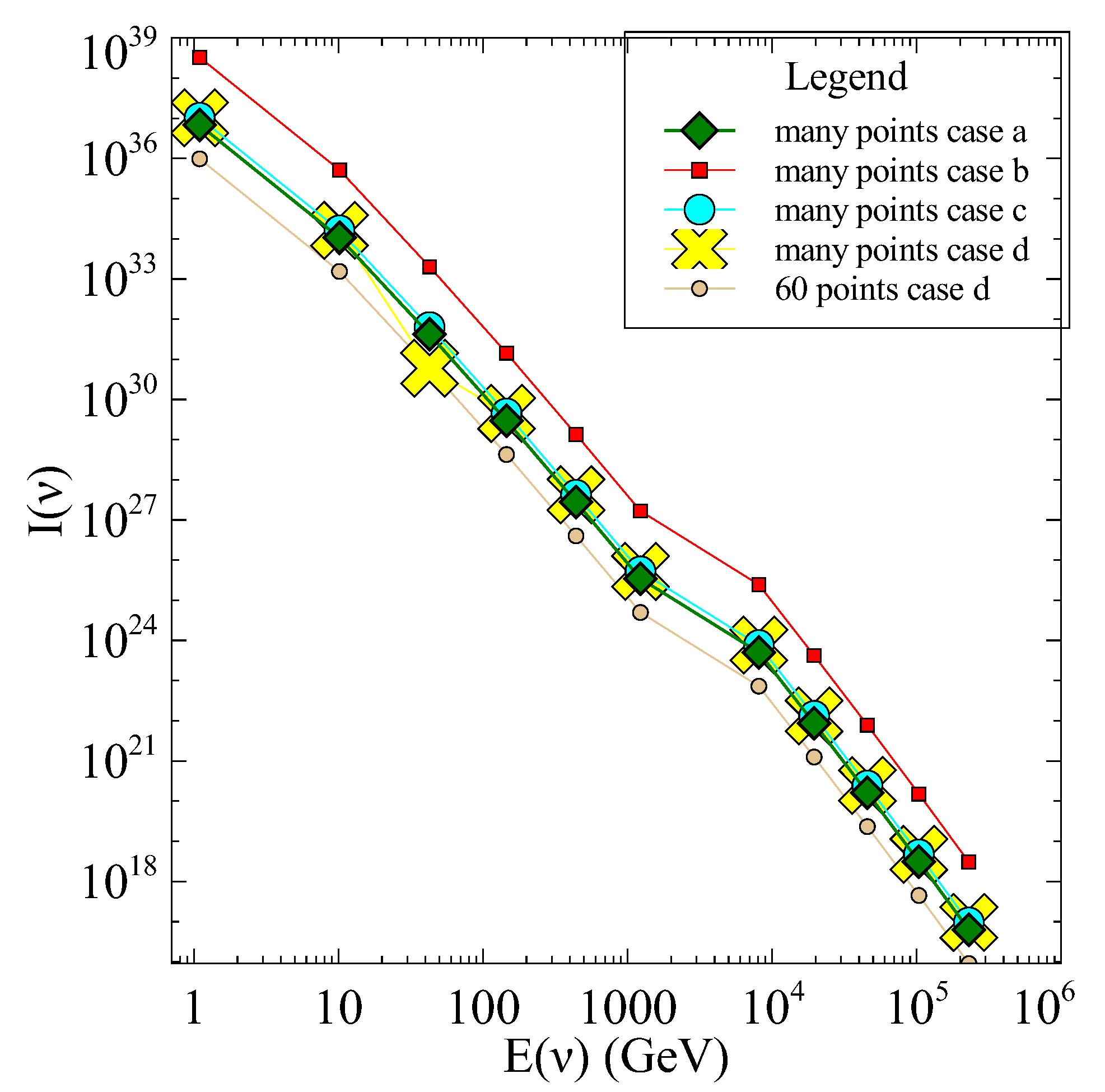
Figure 8.
Example distance-dependent detectability: horizon distance for selected instruments, derived from the model flux at and instrument sensitivities.
Figure 8.
Example distance-dependent detectability: horizon distance for selected instruments, derived from the model flux at and instrument sensitivities.
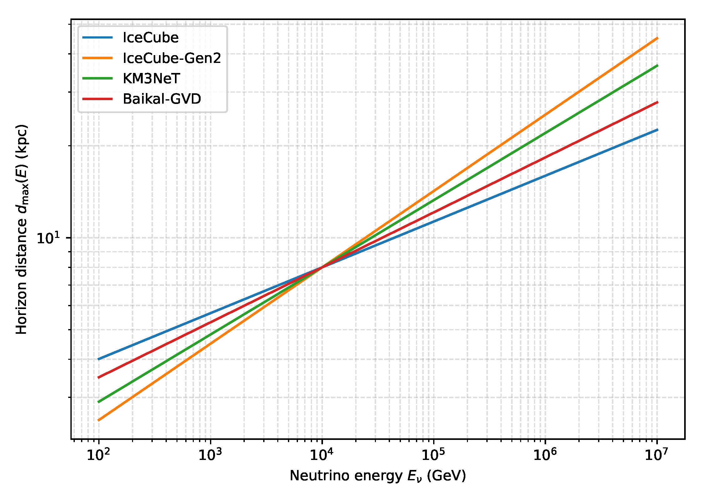
Figure 9.
Total neutrino emissivity versus model time at 1.096 GeV neutrino energy. Transient behavior corresponds to consecutive jet plasmoid injections and exits.
Figure 9.
Total neutrino emissivity versus model time at 1.096 GeV neutrino energy. Transient behavior corresponds to consecutive jet plasmoid injections and exits.
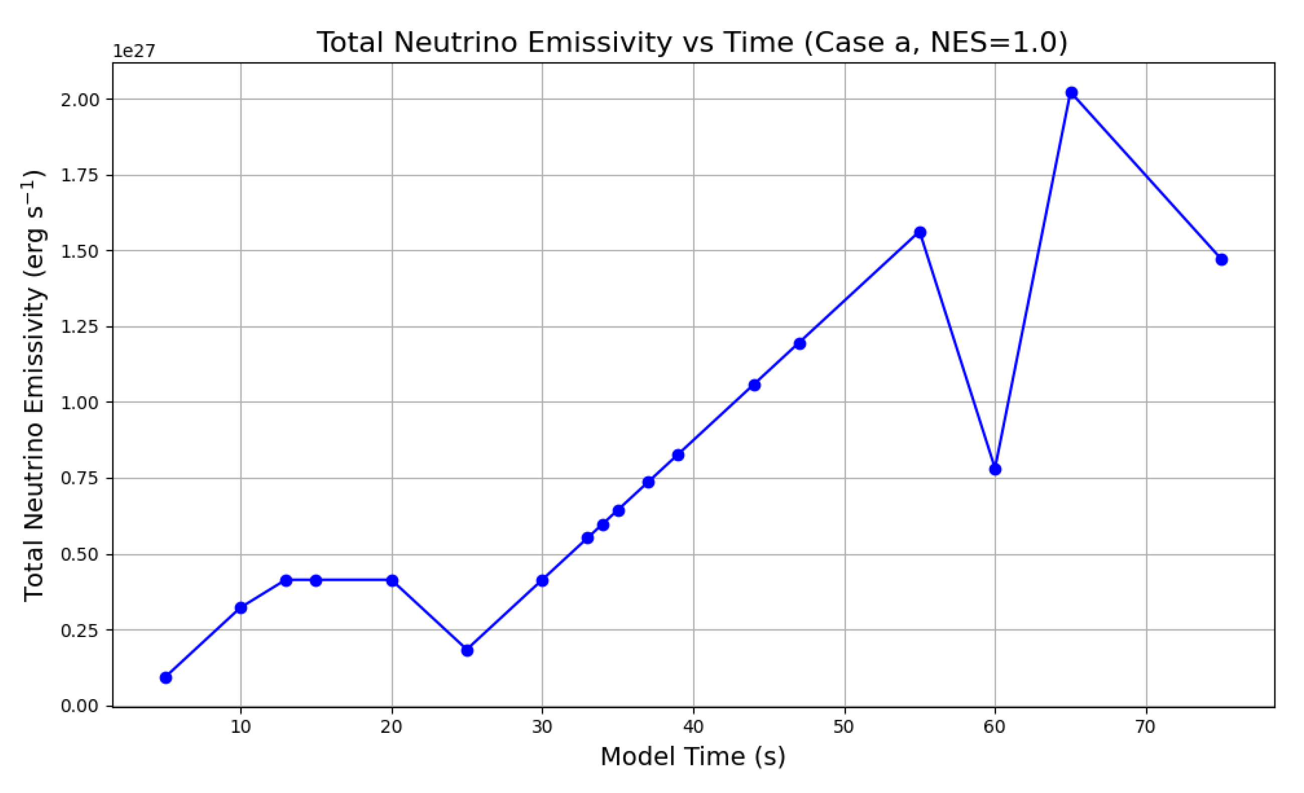

Table 1.
Simulation and Model Parameters.
| Parameter | Value | Comments |
| Cell size | cm | PLUTO cell length |
| Jet density | Jet proton density | |
| Wind max density | Max ambient wind density | |
| Disk wind max density | Max disk wind density | |
| Time unit | 1 s | Model time scale |
| Max run time | 204 s | Total simulation time |
| Integrator | MUSCL-Hancock | PLUTO scheme |
| Physics | Special Relativistic MHD | RMHD setup |
| Initial magnetic field | G | Toroidal field |
| Binary separation | cm | |
| Jet kinetic luminosity | erg/s | Jet power |
| Jet speed | 0.8 | Jet velocity fraction of c |
| Grid size | PLUTO mesh size | |
| Imaging method | Focused beam | rlos configuration |
| Imaging plane | YZ plane | Fiducial screen orientation |
| Emission type | Neutrinos | Synthetic emission mode |
Disclaimer/Publisher’s Note: The statements, opinions and data contained in all publications are solely those of the individual author(s) and contributor(s) and not of MDPI and/or the editor(s). MDPI and/or the editor(s) disclaim responsibility for any injury to people or property resulting from any ideas, methods, instructions or products referred to in the content. |
© 2026 by the author. Licensee MDPI, Basel, Switzerland. This article is an open access article distributed under the terms and conditions of the Creative Commons Attribution (CC BY) license (http://creativecommons.org/licenses/by/4.0/).
Copyright: This open access article is published under a Creative Commons CC BY 4.0 license, which permit the free download, distribution, and reuse, provided that the author and preprint are cited in any reuse.


