Submitted:
16 January 2026
Posted:
19 January 2026
You are already at the latest version
Abstract
This work presents the development and validation of a 1D, co-flow, finite-volume model for the simulation of planar SOFCs, developed for integration in more complex systems and process simulations. The model is calibrated and validated using experimental SOFC polarization curves in a wide range of operating conditions in terms of H2 and H2O molar fraction in the fuel, temperature, and fuel utilization factor, demonstrating good accuracy and the possibility to simulate the most relevant physical processes occurring within an SOFC and to investigate its internal operating conditions in terms of temperature, current density, and gas composition profiles.
Keywords:
solid oxide fuel cell
; 1D SOFC model
; channel-level model
; finite-volume model
1. Introduction
Solid oxide fuel cells (SOFCs) and solid oxide electrolysis cells (SOECs) are emerging energy conversion technologies that can support the energy transition. Their use can improve the efficiency of existing energy conversion concepts, like in the case of an SOFC used for cogeneration applications, or prompt the development of new concepts, like multi-energy systems based on reversible solid oxide cells (rSOCs) [1], or hybrid power generation systems integrating an SOFC with gas or steam cycles [2]. Modern SOCs operate at a high temperature between 600 °C-800 °C using in most cases a solid yttria-stabilized zirconia (YSZ) electrolyte. On the one hand, the high temperatures bring several advantages compared to similar electrochemical devices based on polymeric or alkaline electrolytes, including higher efficiency, the possibility of thermal integration at system level, fuel flexibility, and absence of expensive catalysts. On the other hand, the main drawbacks include a faster degradation of the cell main components and the need to carefully manage internal thermal gradients.
Using accurate models to predict the performance of SOFC (or SOEC) is a crucial aspect for the development of energy systems based on this technology. In general, a stationary SOFC model includes mass and energy balances to find the internal gas composition and temperature profiles, and an electro-chemical model to calculate the local rate of electrochemical and chemical reactions. The model dimensionality and complexity can vary substantially, including 1D approaches developed along the main direction of the gas flows [3], 1D+1D or 2D models with a refined description of the processes occurring within the electrodes [4] and at the cell layer boundaries, and 3D models of the solid oxide cell (or stack) using commercial software like COMSOL [5] and CFD (computational fluid-dynamics) approach. The review work of Wu et al. [6] provides an in-depth description of the available SOFC models, highlighting strengths, weaknesses, and field of application for each of them. In particular, 1D models can be more easily integrated into wider system simulations due to the significant computational burden of 2D and 3D models, allowing the system optimization while retaining a good description of physical processes occurring within the stack. Two- and three-dimensional models provide additional insights on the stack internal operating conditions and can improve the performance estimation, especially at high current density [7].
This work presents an updated version of a 1D, co-flow, finite-volume model for the simulation of planar SOFCs, that has been already validated and used in several works [3,8]. Differently from previous versions, the model is developed to allow running within Aspen Plus® for wider system and process simulations; the Aspen environment provides built-in functions for the calculation of physical and thermodynamic properties of gases and facilitates the model integration.
The model developed is calibrated and validated using experimental polarization curves of an SOFC, covering a wide range of operating conditions in terms of H2 and H2O molar fraction in the fuel, temperature, and fuel utilization factor (exceeding 90%), which is not common for relatively simple 1D models. The experimental data are reported in ref. [4], which also includes a numerical investigation using a 1D+1D model integrating the dusty gas model (DGM) for species diffusion in the electrode, and a distributed electrochemical model applied throughout the electrode thickness. One of the aims of this work is to demonstrate that the same set of data can be described by a simpler 1D model over a wide range of operating conditions, drastically reducing complexity and computational time, facilitating the grid convergence, while retaining a good accuracy.
2. Model Description
The model developed is designed for the simulation of standard solid oxide cells using Y-doped zirconia as electrolyte. The electrochemical reactions (1) and (2), representing the hydrogen oxidation reaction (HOR) and the oxygen reduction reaction (ORR), occur at the fuel and air electrode, respectively. In fuel cell mode, H2 is oxidized to H2O, consuming an oxygen ion in the electrolyte and producing two electrons in the electronic-conducting phase (e.g., nickel). Electrons flow through an external resistance towards the positive electrode (air electrode), where they combine with oxygen to produce an oxygen ion in the electrolyte. The HOR and the ORR proceed forward and backward in fuel cell and electrolysis mode, respectively.
Figure 1 (left) shows a generic solid oxide cell stack made of multiple planar cells stacked on top of each other, each cell containing several gas channels as the one shown in the right-hand side of Figure 1. The model developed in this work considers a single channel as geometric domain, assuming that the whole stack (or cell) can be represented by a number of identical channels, which significantly limits the model complexity. The finite-volume model developed is one-dimensional in the direction of the channel; it assumes steady-state operation, co-flow arrangement, and it can be used to model both fuel cell and electrolyzer modes. The model is implemented in Aspen Plus® environment, which allows exploiting a built-in equations solver and accurate datasets for the calculation of thermodynamic and physical properties of gas mixtures.
The model inputs are the channel geometry, the conditions of the inlet streams (temperature, composition, pressure, and mass flow rate), several parameters required to model the physical processes, and the cell voltage, which is assumed to be constant throughout the channel (electrode equipotential assumption). The main outputs of the 1D model are the distribution along the axial direction of:
- The composition () and temperatures ( and ) of the gas streams;
- The temperature () of the Positive-Electrolyte-Negative (PEN) structure (i.e., assembly including the electrodes and the electrolyte);
- The temperature of the interconnect at the fuel side and air side ( and );
- The current density () and the electrochemical overpotentials ().
Figure 2 shows the main dimensions defining the channel geometry, which also allow to define the relevant geometrical parameters shown in Table 1.
The finite-volume solution algorithm includes the division of the channel in N small pieces as the one shown in Figure 3 (left), which will be called control volume (CV). Assuming that the cell voltage is fixed throughout the channel, the electrochemical model allows to calculate the local current density , which is equal to the small (but finite) current () flowing through the interconnects of the CV divided by the active area contained in it (), as shown in Eq. (3).
The electrochemical model developed is zero-dimensional, meaning that electrochemical reactions are assumed to only occur at the interface between the electrode and the bulk of the electrolyte. Coherently with the use YSZ as electrolyte, short-circuit electronic currents in the electrolyte are neglected, hence the current collected by the interconnects is equal to the ionic current flowing in the electrolyte.
As shown in Figure 3 (right), each CV is further divided into 5 sub-volumes enclosing the fuel and air channels, the interconnects, and the PEN structure. Mass and energy balances are solved for each of these 5 x N sub-volumes to find the temperature and gas composition along the channel. A uniform temperature is defined for the solid parts (interconnects and PEN sub-volumes) of each CV, resulting in 3 x N unknown temperatures. The fuel and air temperatures at the outlet interface of each CV are also unknown, resulting in 5 x N unknown temperatures in total, which is equal to the number of energy balance equations.
Axial heat conduction in the direction is considered for the PEN and the interconnects, while it is neglected for gas streams due to the low thermal conductivity of the gases. In the direction, only the convective heat exchange between gases and interconnects is considered (with exchange area per unit length equal to ). The heat exchange in the direction includes the convective heat transfer between gases and solid parts, the conductive heat transfer between PEN and interconnects, and the heat loss which is assumed to be uniformly distributed on the external interconnect surfaces. The radiative heat exchange between PEN and interconnects is neglected since the temperature of the solid parts are always found to be very similar in the and directions even when radiative heat exchange is not considered, while the view factors are very small in the direction.
The main equation used for the calculation of the local current density is the voltage balance shown in Eq. (4). The cell voltage () is fixed (if the total current is fixed, instead of the voltage, the same model can be run iteratively to find the voltage which matches the required current), and is the ideal maximum (minimum) cell voltage in fuel cell (electrolysis) mode. The term depends on temperature, and a simple correlation can be derived by fitting thermodynamic data [3]. The partial pressures of hydrogen and steam ( and used in Equation (5) are those found locally in the fuel channel; similarly, the local oxygen partial pressure in the air channel () is used. The overpotentials shift the cell voltage from the ideal value, decreasing its performance. In the model developed, both the overpotentials and the current density are positive in fuel cell mode and negative in electrolysis mode. All the overpotentials depend on the current density, and Eq. (4) is used to implicitly calculate .
Equation (6) is used to calculate , which accounts for the fact that the measured open-circuit voltage (OCV) is typically slightly lower compared to the ideal value calculated with Equation (5), even if the external current is null [4,9]. This might be due to small gas leaks or a short-circuit electronic current within the electrolyte. In fuel cell (or electrolysis) mode the maximum current density is calculated assuming that all the equivalent hydrogen (or steam) is consumed, generating a corresponding faradaic current. Therefore, the leakage loss is important near the OCV and tends to zero when the current density is large (in absolute value).
The concentration overpotential, which is calculated with Eq. (7), accounts for the fact that the ideal voltage should be calculated using the species partial pressures in the proximity of the reaction site (i.e., , , and ), here assumed located at the electrode-electrolyte interface. Assuming that the total pressure is constant throughout the electrodes, the partial pressures in Eq. (7) can be replaced by molar fractions.
The molar fractions of H2, H2O, and O2 at the electrode-electrolyte interfaces are calculated using Eqs. (8), (9), and (10) [10]. The coefficient is included to account for the fact that the reference surface for the diffusion process is lower than the active area.
The binary diffusion coefficients are calculated according to the Fuller method, which is valid for pressures below 35 bar [11]. The effective molecular diffusion coefficients in the gas mixture are then calculated with Eq. (11), which assumes that the species diffuses in subsequent gas layers, where each layer has a thickness proportional to and a binary diffusion coefficient . The effective Knudsen diffusion coefficient is calculated with Eq. (12), and the overall diffusion coefficient in the porous electrode is calculated using Eq. (13), which assumes that molecular and Knudsen diffusion occur in series. The parameter is the average pore radius, and is the molar mass of species .
The ohmic loss is calculated with Eq. (14), where the main contribution is due to the oxygen ion conductivity () along the electrolyte thickness (), and is a calibration parameter that can be used to fit the data, representing an additional electric contact resistance which includes the effect of the interconnects (material electric resistance and contact resistance) and other contributions that are not (or cannot be) explicitly considered in the model.
The activation overpotentials in the fuel electrode () and air electrode () are calculated using Butler-Volmer equations (16) and (18), and their sum is equal to the overall activation overpotential (). The form of the Butler-Volmer equations is taken from [4], and both and are referred to the active area of the cell.
The mass balance equation for each species can be written in differential form as shown in Equation (20), accounting for possible chemical or electrochemical reactions and the stoichiometric coefficient of species in reaction . The reaction rate (mol s-1 m-2) is specific to the active area of the cell. The sum of the HOR and the ORR can be considered as a single overall reaction whose reaction rate is calculated as in Eq. (21), with stoichiometric coefficients equal to -1, 1, and -0.5 for H2, H2O, and O2, respectively.
Concerning water gas shift (WGS) and methane steam reforming (MSR) reactions, a global reaction approach described by Eqs. (22) and (23) is used. In this work, the WGS reaction is assumed to be equilibrated throughout the channel. In particular, the forward kinetic constant is fixed to an arbitrarily large value, the partial pressures in Eq. (22) are those at the outlet of each CV, and is calculated using the fuel temperature at the outlet of each CV. In this way, the species partial pressures are guaranteed to satisfy the WGS equilibrium condition throughout the channel. Assuming that the inlet fuel composition is already in equilibrium, which is typically the case for pre-reformed gas mixtures, using the fuel temperature to calculate also allows to avoid a step-wise change in composition that would arise in case the PEN temperature was used.
Regarding the MSR reaction, the kinetic model reported by Timmermann et al. is selected [12]. This model is valid in the range 600 °C-750 °C, which is in line with the operating temperature of modern SOFCs; the temperature at cell outlet might be even larger, but methane is typically consumed near the inlet section of the cell. The pre-exponential factor appearing in the kinetic constant , which is equal to 1483 mol s-1 m-2 in the original reference, is scaled by a factor 1.73 to refer to the active area instead of the surface touched by the gas. The scaling factor is derived from the channel width () and interconnect thickness () stated in ref. [12], equal to 1.5 mm and 0.55 mm, respectively. Note that both and are calculated using the local PEN temperature.
Equations (24)-(28) represent the energy balances for the fuel channel, air channel, PEN assembly, fuel-side interconnect, and air-side interconnect, respectively. The energy exchanges between gas and solid parts are further detailed in Table 2. The left-hand side of Eqs. (24) and (25) represents the variation of enthalpy flow along the axial coordinate, where and are the overall molar flow rate at the fuel and air side, respectively, and the specific enthalpy, which is calculated using Peng-Robinson correlations imported from Aspen Plus®, is a function of the local gas composition and temperature. The left-hand side of Eqs. (26), (27), and (28) accounts for the axial conduction of the solid parts. A heat loss term , expressed in W m-2, is also included in Eqs. (28) and (29), and it is specific to the interconnects surfaces facing adjacent cells. All other external surfaces of the channel are assumed to be adiabatic.
The local convective heat transfer coefficients () for the fuel and air streams are calculated from the local gas thermal conductivity and the hydraulic diameter of the channels, and assuming constant Nusselt numbers. The PEN thermal conductivity is calculated as shown in Eq. (30).
3. Results and Discussion
3.1. Model Calibration and Validation
The experimental data on commercial 5 x 5 cm2 (4 x 4 cm2 active area) cells, reported by Neri et al. [4], is used to validate the model. The cell is manufactured by Elcogen and it is composed by a thick Ni-YSZ composite electrode (400 μm), a thin YSZ electrolyte (1.5 μm), a GDC (Ce0.9Gd0.1O2-δ) barrier layer (1.6 μm), and a LSC (La0.6Sr0.4CoO3-δ) single-phase cathode (15 μm). The experimental polarization curves used for the model validation cover a wide range of operating conditions:
- 7% humidified fuel gas mixtures with 21%-93% H2 fraction and N2 balance at 750 °C;
- 50% H2 fuel gas mixtures with 10%-50% steam content and N2 balance at 750 °C;
- 7% humidified fuel gas mixture with 93% H2 fraction at 550 °C-700 °C.
A large excess of air (assumed composition is 21% O2 and 79% N2) is always used at the cathode side of the cell. Note that the limiting current density is approached when the H2 fraction is low, allowing to evaluate the model performance at large fuel utilization factors typical of real applications. More detailed information on the cells, the experimental setup, and the experimental procedures are available in ref. [4].
Since the cell was placed in a furnace with a fixed setpoint temperature, the temperature distribution is assumed uniform throughout the channel length for all gas and solid parts. As demonstrated by Neri et al., this hypothesis can be justified by the inconsistent results stemmed from the assumption of adiabaticity, and the large thermal conductivity of the nickel current collector, which efficiently dissipates the heat produced by electrochemical reactions.
Table 3 summarizes the main parameters used for model validation. Most of the values are derived from ref. [4], while several parameters are calibrated. The ohmic parameters and are calibrated from EIS data shown in ref. [4]; note that the contact resistance grew significantly as a consequence of a blackout (15 min) when passing from experiments at low temperature to 750 °C, therefore, two values of are calculated (the blackout only affected the ohmic resistance of the cell). The remaining 8 parameters are calibrated using the polarization curves, and include the activation loss parameters, the anode tortuosity, and the inlet fuel flow rate. Note that there is uncertainty about the fuel flow rate that actually reaches the cell due to leakages on the fuel pathway and in the fuel distributor (the experimental setup avoids using sealings, which may damage the cells during disassembling), which justifies its inclusion in the set of calibrated variables. The calibrated inlet fuel flow rate is equal to 5.486 Nml min-1 cm-2, which is similar to the 6.25 Nml min-1 cm-2 value indicated in ref. [4].
Figure 4 shows the experimental polarization curves and the model predictions for different H2 and H2O concentrations (panels a and b), and different temperatures (panel c). At each cell voltage, the average current density is calculated by the model with Eq. (31).
Considering the wide range of operating conditions investigated in terms of reactants concentrations, temperature, and fuel utilization, the good matching between model and experiments demonstrates the generality of the model developed. Notably, the model accuracy is not significantly worse compared to the results shown in ref. [4], where the same set of data is described using a 1D+1D model which couples the dusty gas model with a distributed electrochemical model along the electrode thickness for a better representation of ohmic and activation overpotentials.
The measured OCV is always 6-24 mV lower compared to the theoretical value . Therefore, the leakage loss calculated with Eq. (6) is limited. The limiting current is approached for the case with 21% H2, as 95.6% of the available hydrogen is consumed near 0.7 V. Notably, the model correctly predicts the cell performance also in this extreme case, where concentration losses plays a major role.
Figure 5 shows the average overpotentials, calculated using Eq. (32), in different selected operating conditions. Note that since the overpotentials represent the exergy lost per unit charge (J C-1), they are weighted by the local current produced. The oxygen concentration loss is not shown in the figure since it is negligible in all cases, and the anode concentration loss includes contributions from both H2O and H2 diffusion processes in the electrode.
Panel a shows the overpotentials for the case with 7% H2O and 21% H2 (N2 balance) at 750 °C, and suggests that the concentration loss always dictates the cell performance. Although it is not shown, most of the anode concentration loss is due to steam diffusion in the low current density region since its concentration in the channel is low compared to hydrogen. In other words, if or in the channel are low, or can be very different from their channel values percentage-wise, significantly increasing the concentration polarization (see Eqs. (7), (8), and (9)). The H2 concentration polarization becomes dominant only above 125 mA cm-2 due to the fuel depletion, and it grows exponentially at larger current densities. Since the calibrated H2 exponent (coefficient in Table 3) is equal to 0.5, the anode activation loss grows significantly at large current densities. The anode tortuosity has been calibrated by closely matching the cell performance at low current densities due to the dominance of concentration losses in this region.
Panel b shows the overpotentials calculated for the case with 50% H2 and 50% H2O at 750 °C. Concentration losses are limited due to the large channel concentration of both H2 and H2O. Hydrogen and steam diffusion processes contribute approximately equally to the anode concentration loss, since is large even at low current densities, and the H2 utilization factor is limited in the high current region (78% at 0.7 V). Anode activation and ohmic overpotentials have the greatest impact on the cell performance.
Panel c shows the polarization losses for the case with 93% H2 and 7% H2O at 550 °C. The concentration overpotential gives the smallest contribution to the cell polarization due to the relatively weak dependence of diffusion processes on temperature. Contrarily, the cathode activation overpotential grows significantly, being the most important contributor together with the anode activation loss.
In general, the trends discussed and the overpotentials calculated are similar to those shown in ref. [4], suggesting that both models can be used for the simulation of solid oxide fuel cells.
Note that there are instances where the sum of the molar fractions of steam () and hydrogen () in the reaction site is above 1 (e.g., in the case with 50% H2 and 50% H2O at high current density), which could raise concerns on the modified Fick’s model used (Eqs. (8) and (9)) compared to the rigorous dusty gas model approach employed in more sophisticated SOFC models. Nevertheless, the model remains consistent since and shall not be intended as accurate estimations of the molar fractions in the reaction site, but only be used to calculate the partial pressures and . The sum of the partial pressures at the reaction site is indeed allowed to exceed the total pressure in the channel (i.e., the total pressure in the electrode can be larger compared to the channel value), and their values are in good agreement with those found with the DGM model, as discussed with more detail in the Appendix A.
3.2. Adiabatic Model with Reformate Fuel
In order to test the adiabatic model (which also includes energy balances) in a condition representative of a real application, the operating conditions calculated in ref. [2] are considered. In particular, Table 4 shows the operating conditions of an SOFC integrated in a hybrid power generation system which also includes a bottoming steam cycle.
The global heat loss assumption is used to calculate (see Eqs. (28) and (29)), which is equal to 40 W m-2. The investigated operating conditions are peculiar because of the low inlet fuel temperature equal to 521 °C, which might cause significant thermal gradients near the SOFC entrance. All parameters shown in Table 3 are used for the simulation, with some exceptions:
- The inlet fuel and air mass flow rates at channel inlet are derived to match the fuel utilization factor and the outlet cell temperature stated in Table 4;
- The channel length is set to 9 cm, which is a value in line with applicative cells, the channel width is fixed to 3 mm for the same reason;
The parameter
- is fixed to 464167 S K m-1 (used for the simulations in Figure 4c).
The thermal conductivity of the anode, cathode, and electrolyte (, , ) is fixed to 2 W m-1 K-1, while the interconnect conductivity () is equal to 20 W m-1 K-1. The Nusselt number is fixed to 3.6 and 5.0 in the fuel and air channels, respectively [3].
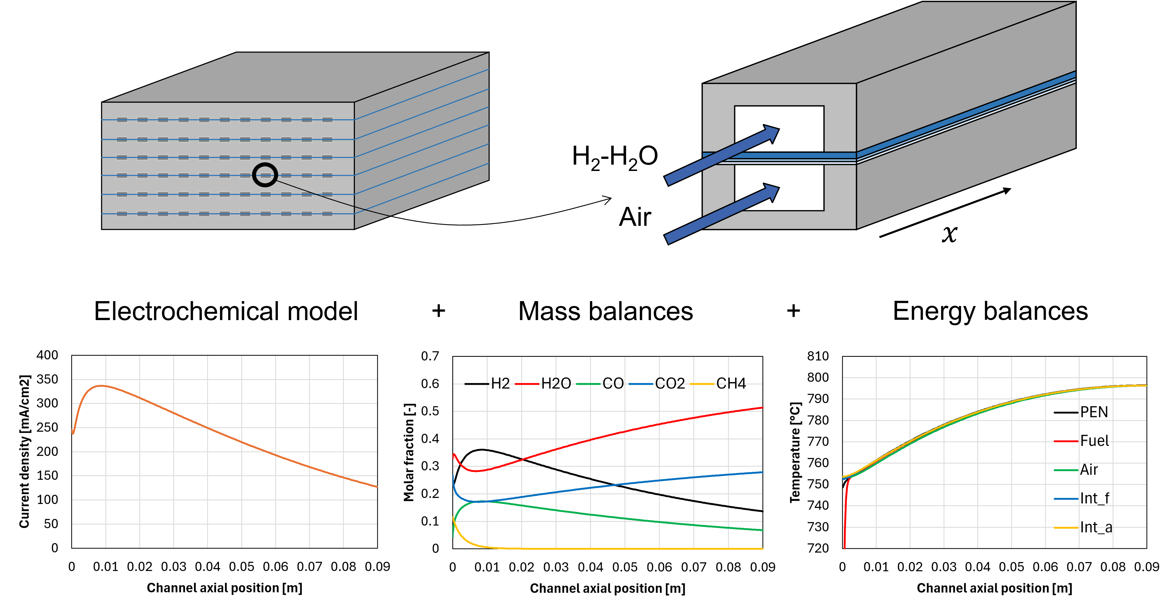
Figure 6 shows the results of the adiabatic simulation. Panel a shows the temperature profiles calculated for the PEN, interconnects, and gas streams. Although the fuel inlet temperature is equal to 521 °C, the minimum value of the temperature axis is fixed to 720 °C for clarity.
The fuel reaches a temperature close to that of the air stream almost instantly, which is due to its relatively low thermal inertia (the inlet air molar flow rate is 5.42 times larger). The PEN temperature near the channel inlet seems to be the only one slightly affected by the low fuel temperature; this is attributed to its relatively large resistance to axial conduction, since the temperature of the fuel interconnect is higher despite having a larger contact surface with the fuel stream. The PEN temperature remains large due to the heat exchange with the air stream and the interconnects, but there is a very small region where the PEN temperature gradient reaches 4 °C mm-1, which is a large value if compared with the one calculated in the middle of the channel, equal to 0.5 °C mm-1.
Panel b shows that the current density reaches a maximum value near the channel entrance, which corresponds to the H2 concentration peak shown in panel c. After this point, the current density decreases due to H2 depletion and H2O formation, despite the increasing temperature trend. Panel c shows that methane is rapidly consumed producing H2, overcompensating the H2 consumed by electrochemical reactions up to the peak already mentioned. The existence of a H2 concentration peak near the channel inlet is typical of SOFCs operating with reformate, as also demonstrated in other modelling works [3,8].
Panel d shows the effect of grid refinement on the PEN temperature distribution. Since the PEN temperature frequently appears both in the electrochemical, chemical, and energy balance models, it is considered representative of the status of all other calculated variables. The sensitivity analysis suggests that dividing the channel into 100 control volumes is sufficient to achieve the grid independence.
Overall, the model developed correctly simulates the most relevant physical processes occurring within a SOFC, elucidating the internal operating conditions like the temperature, current density, and gas composition profiles.
It shall be noted that the model is also flexible by the point of view of the cell operating mode, since its extension to the case of electrolysis operation (not sown here for brevity) is straightforward and does not require any mathematical modification; in the electrolysis case, the cell voltage assigned in input is larger than the Nernst voltage, resulting in a negative current density calculated by the electrochemical model.
4. Conclusions
This work presented the development and validation of a 1D, co-flow, finite-volume model for the simulation of planar SOFCs. The model is developed to facilitate the SOFC simulation in wider system and process simulations in Aspen Plus®, which provides built-in functions for the calculation of physical and thermodynamic properties of gases.
The model allows to simulate the most relevant physical processes occurring within an SOFC and to investigate its internal operating conditions in terms of temperature, current density, and gas composition profiles. The model is calibrated and validated using experimental SOFC polarization curves covering a wide range of operating conditions in terms of H2 and H2O molar fraction in the fuel, temperature, and fuel utilization factor. The discussion demonstrates that the dataset can be described by the 1D model over a wide range of operating conditions, drastically reducing complexity and computational time compared to more complex multi-dimensional models, facilitating the grid convergence, while retaining a good accuracy. The same model can also be used in the case of electrolysis operation without substantial modifications.
Author Contributions
Conceptualization, A. C., P. C., S. C.; methodology, software, validation, formal analysis, investigation, data curation, writing—original draft preparation, visualization, A. C.; writing—review and editing, A. C., P. C., and S. C.; supervision, project administration, funding acquisition, resources, P. C. and S. C. All authors have read and agreed to the published version of the manuscript.
Funding
This research received no external funding.
Data Availability Statement
Data is contained within the article or supplementary material.
Conflicts of Interest
The authors declare no conflicts of interest.
Abbreviations
| CV | Control Volume |
| DGM | Dusty Gas Model |
| EIS | Electrochemical Impedance Spectroscopy |
| HOR | Hydrogen Oxidation Reaction |
| MSR | Methane Steam Reforming |
| OCV | Open Circuit Voltage |
| ORR | Oxygen Reduction Reaction |
| PEN | Positive-Electrolyte-Negative |
| SOC | Solid Oxide Cell |
| SOEC | Solid Oxide Electrolysis Cell |
| SOFC | Solid Oxide Fuel Cell |
| WGS | Water Gas Shift |
| YSZ | Yttria-Stabilized Zirconia |
Appendix A
Calculation of H2 and H2O partial pressure at cell reaction site
Estimating the quantity of reacting species reaching the cell reaction sites is one of the key steps in the solid oxide cell model; in particular, the partial pressures of hydrogen and steam directly influence the concentration overpotential (Eq. (7)) and the activation overpotential (Eq. (17)).
The most referenced approach to evaluate the variation of partial pressure from the bulk region of the cell channels to the actual reaction sites, due to the diffusion process in the porous electrode structure, is the Dusty Gas Model (DGM).
Diffusion of each species through the porous electrode according to the DGM can be expressed by Eq. (33). In Eq. (33), the terms are the species molar fluxes (mol m-2 s-1), and is the electrode permeability; both molecular and Knudsen diffusion coefficients are intended as effective coefficients, meaning that they are already multiplied by .
This set of equations cannot be solved analytically in its complete form. Assuming a H2-H2O fuel gas mixture (), equimolar counter-diffusion (), and neglecting the term including the electrode permeability, it is possible to derive Eqs. (34) and (35):
The integration along the fuel electrode thickness ( direction) then gives Eqs. (36) and (37), where the molar fluxes are expressed in terms of current density.
Equations (8) and (9) for the estimated molar fractions and can then be derived assuming that the total pressure along the electrode is equal to the channel total pressure, introducing an approximation error (the error derives from neglecting the total pressure derivative term which appears from the expansion of the right-hand side of Eqs. (34) and (35)). However, when and calculated with Eqs. (8) and (9) are multiplied by the channel total pressure, the partial pressures found are the same as the ones calculated with Eqs. (36) and (37). Therefore, and calculated with Eqs. (8) and (9) should only be used for the calculation of and by multiplying by the channel total pressure, and they should not be intended as accurate estimations of the molar fractions in the reaction site.
For multi-component gas mixtures, the functional form of Eqs. (36) and (37) is assumed to remain the same, but and are calculated using and (calculated with Eq. (11)) instead of .
Figure A1 shows , , , and calculated with the rigorous DGM and with the Fick’s model (Eqs. (8) and (9) assuming equal to 1), for different H2 molar fractions in the fuel (balance H2O). Since atmospheric pressure (1.01 bar) is assumed in the channel, molar fractions and partial pressures are almost the same in the Fick’s model, hence only molar fractions are shown in the figure. The current density is always assumed equal to 1000 mA cm-2, and the fuel electrode parameters shown in Table 3 are used for the calculations. The permeability is equal to 7.84 x 10⁻¹⁷ m2, which is estimated based on the electrode porosity, tortuosity, and particle diameter (assumed equal to 1 μm) [13]. The temperature is assumed equal to 750 °C.
Figure A1.
Molar fractions and partial pressures in the reaction site estimated using the DGM and the Fick’s model, for different H2 fractions in the channel (H2O balance).
Figure A1.
Molar fractions and partial pressures in the reaction site estimated using the DGM and the Fick’s model, for different H2 fractions in the channel (H2O balance).
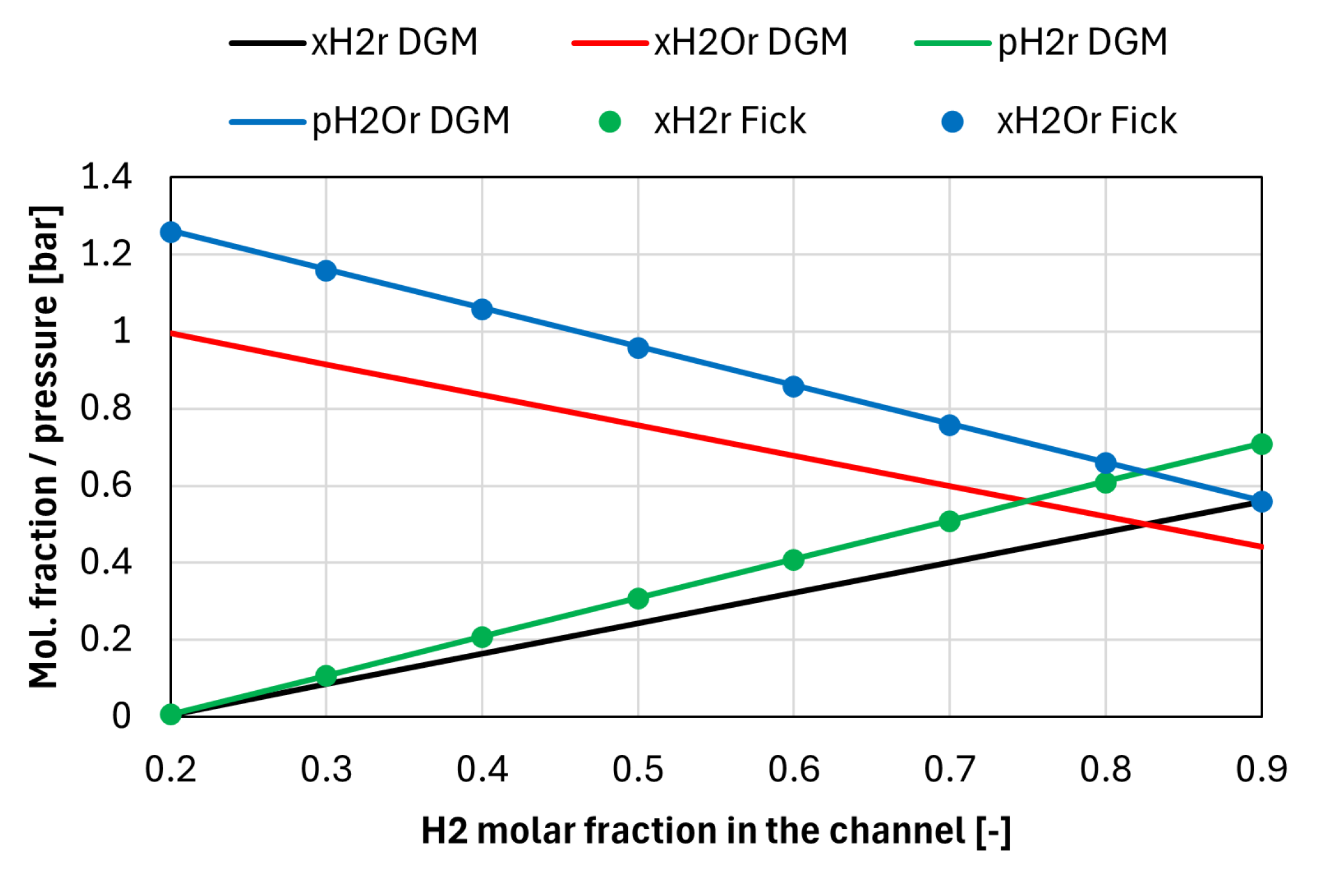
It can be noted that the molar fractions estimated with Eqs. (8) and (9) (represented by the dots in the figure) are by themselves inconsistent since their sum exceeds 1 in all conditions. Therefore, these values should only be used to calculate the partial pressures of H2 and H2O in the reaction site, which yields results having very good agreement with the DGM model, as shown in Figure A1. Note that the total pressure calculated in the reaction site is always equal to about 1.27 bar; indeed the sum of the partial pressures at the reaction site is allowed to exceed the total pressure in the channel (i.e., the total pressure in the electrode can be larger compared to the channel value).
References
- Ficili, M.; Colbertaldo, P.; Campanari, S.; Guandalini, G. Investigating the Partial Load of Reversible Solid Oxide Cell Systems : A Focus on Balance of Plant and Thermal Integration. Appl. Energy 2025, 391, 125876. [CrossRef]
- Campanari, S.; Mastropasqua, L.; Gazzani, M.; Chiesa, P.; Romano, M.C. Predicting the Ultimate Potential of Natural Gas SOFC Power Cycles with CO2 Capture – Part A: Methodology and Reference Cases. J. Power Sources 2016, 324, 598–614. [CrossRef]
- Campanari, S.; Iora, P. Comparison of Finite Volume SOFC Models for the Simulation of a Planar Cell Geometry. Fuel Cells 2005, 5, 34–51. [CrossRef]
- Neri, J.; Cammarata, A.; Donazzi, A. Experimental and Model Investigation of a Solid Oxide Fuel Cell Operated Under Low Fuel Flow Rate. J. Electrochem. Soc. 2023, 170, 124506. [CrossRef]
- Razbani, O.; Assadi, M.; Andersson, M. Three Dimensional CFD Modeling and Experimental Validation of an Electrolyte Supported Solid Oxide Fuel Cell Fed with Methane-Free Biogas. Int. J. Hydrogen Energy 2013, 38, 10068–10080. [CrossRef]
- Wu, Z.; Zhu, P.; Huang, Y.; Yao, J.; Yang, F.; Zhang, Z.; Ni, M. A Comprehensive Review of Modeling of Solid Oxide Fuel Cells: From Large Systems to Fine Electrodes. Chem. Rev. 2025, 125, 2184–2268. [CrossRef]
- Koksharov, A.; Jahnke, T. 3D Modelling of Electrolyzer and Fuel Cells with NEOPARD-X Framework: Dimensionality Effects. In Proceedings of the Proceedings of the European Fuel Cells and Hydrogen Conference; 2025.
- Spallina, V.; Mastropasqua, L.; Iora, P.; Romano, M.C.; Campanari, S. Assessment of Finite Volume Modeling Approaches for Intermediate Temperature Solid Oxide Fuel Cells Working with CO-Rich Syngas Fuels. Int. J. Hydrogen Energy 2015, 40, 15012–15031. [CrossRef]
- Zhu, H.; Kee, R.J. A General Mathematical Model for Analyzing the Performance of Fuel-Cell Membrane-Electrode Assemblies. J. Power Sources 2003, 117, 61–74. [CrossRef]
- Campanari, S.; Iora, P. Definition and Sensitivity Analysis of a Finite Volume SOFC Model for a Tubular Cell Geometry. J. Power Sources 2004, 132, 113–126. [CrossRef]
- Poling, B.E.; Prausnitz, J.M.; O’Connell, J.P. The Properties of Gases and Liquids; 5th ed.; McGraw-Hill Education, 2001;
- Timmermann, H.; Sawady, W.; Reimert, R.; Ivers-tiffée, E. Kinetics of (Reversible) Internal Reforming of Methane in Solid Oxide Fuel Cells under Stationary and APU Conditions. J. Power Sources 2010, 195, 214–222. [CrossRef]
- Zhu, H.; Kee, R.J.; Janardhanan, V.M.; Deutschmann, O.; Goodwin, D.G. Modeling Elementary Heterogeneous Chemistry and Electrochemistry in Solid-Oxide Fuel Cells. J. Electrochem. Soc. 2005, 152, A2427–A2440. [CrossRef]
Figure 1.
Figure 1. Left: solid oxide cell stack made by several cells. Right: single channel within a solid oxide cell. The model developed in this work considers a single channel as the geometrical domain.
Figure 1.
Figure 1. Left: solid oxide cell stack made by several cells. Right: single channel within a solid oxide cell. The model developed in this work considers a single channel as the geometrical domain.
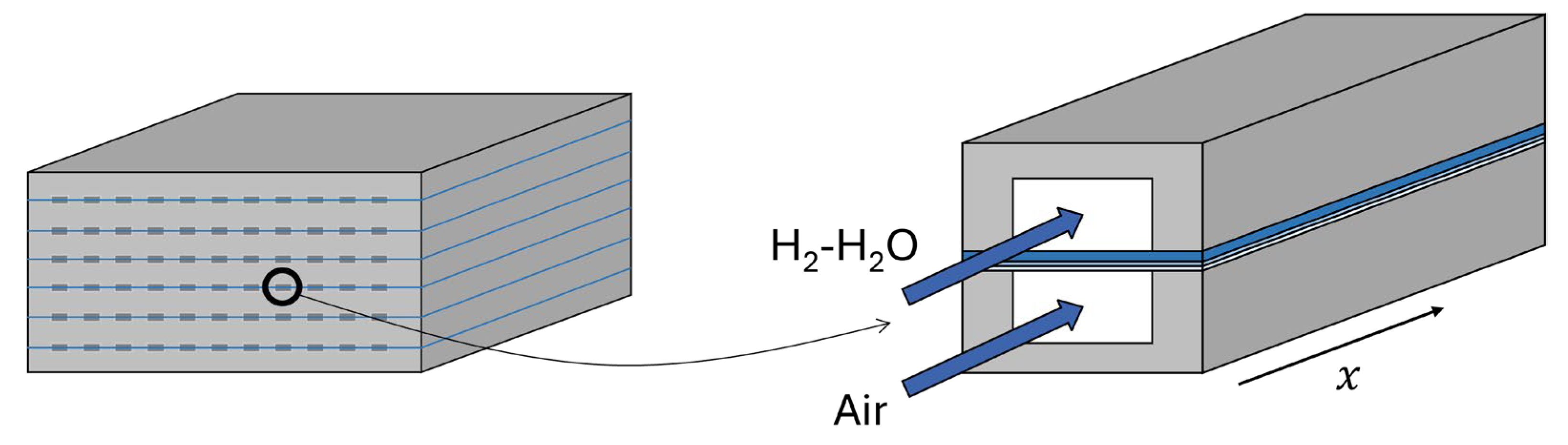
Figure 2.
Figure 2. Main geometrical dimensions of the SOFC channel.
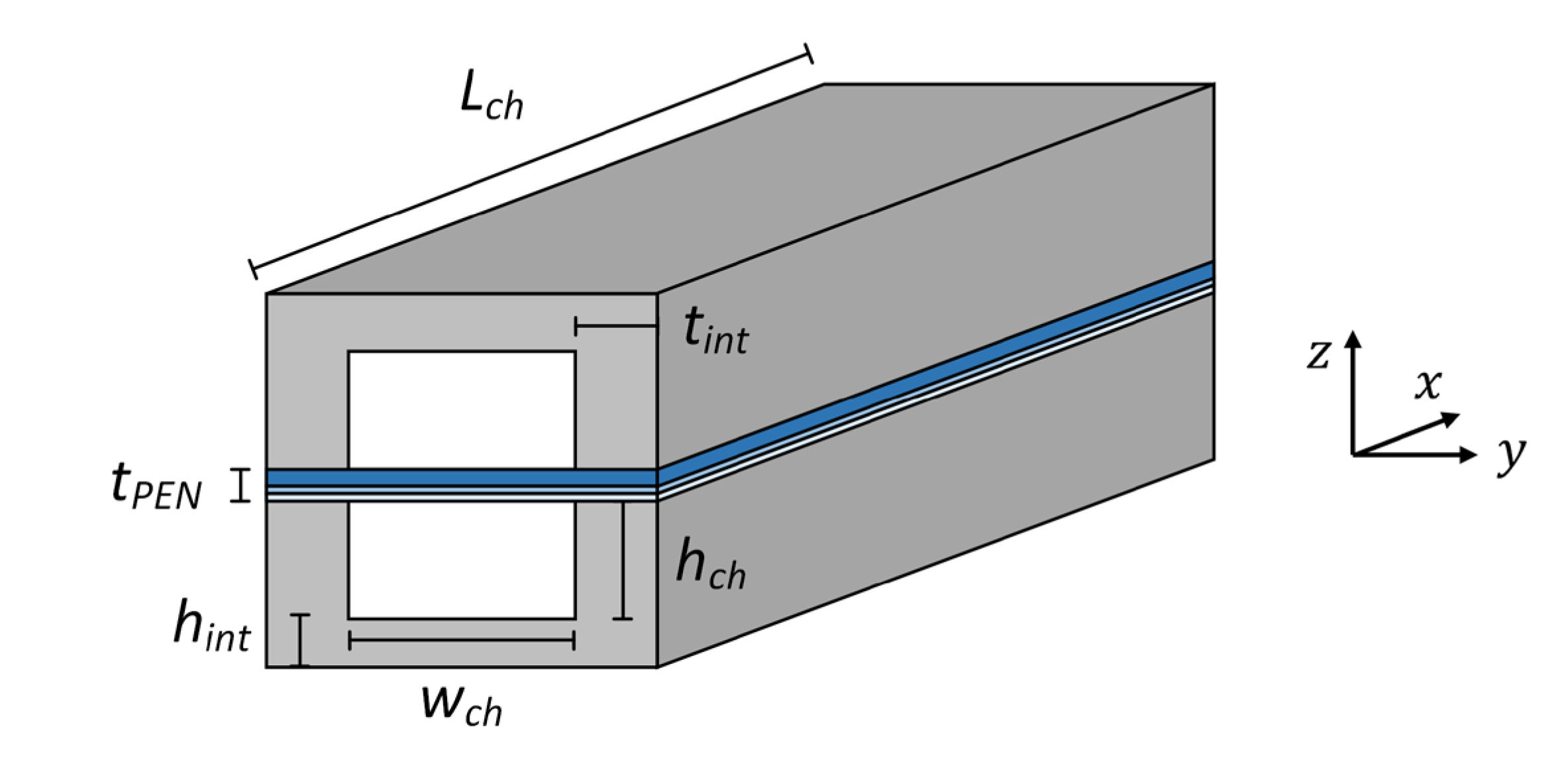
Figure 3.
Figure 3. The channel is divided into N control volumes (left). Each control volume is further divided into 5 sub-volumes (right). The current density is calculated for each control volume, while the energy balances are solved for all 5 x N sub-volumes. Mass balances are solved for the 2 x N sub-volumes enclosing the fuel and air streams.
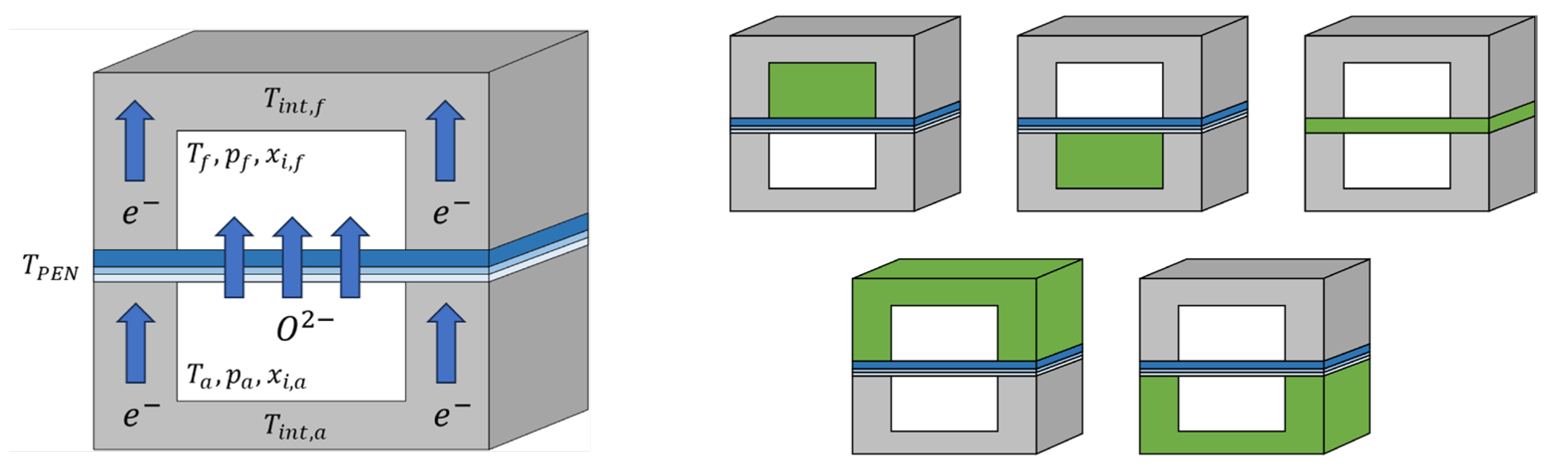
Figure 4.
Figure 4. Experimental polarization curves (dots) and model predictions (lines) at different operating conditions: (a) 7% H2O and 21%-93% H2 (N2 balance) at 750 °C (b) 50% H2 and 10%-50% H2O (N2 balance) at 750 °C (c) 7% humidified H2 at 550 °C-700 °C.
Figure 4.
Figure 4. Experimental polarization curves (dots) and model predictions (lines) at different operating conditions: (a) 7% H2O and 21%-93% H2 (N2 balance) at 750 °C (b) 50% H2 and 10%-50% H2O (N2 balance) at 750 °C (c) 7% humidified H2 at 550 °C-700 °C.
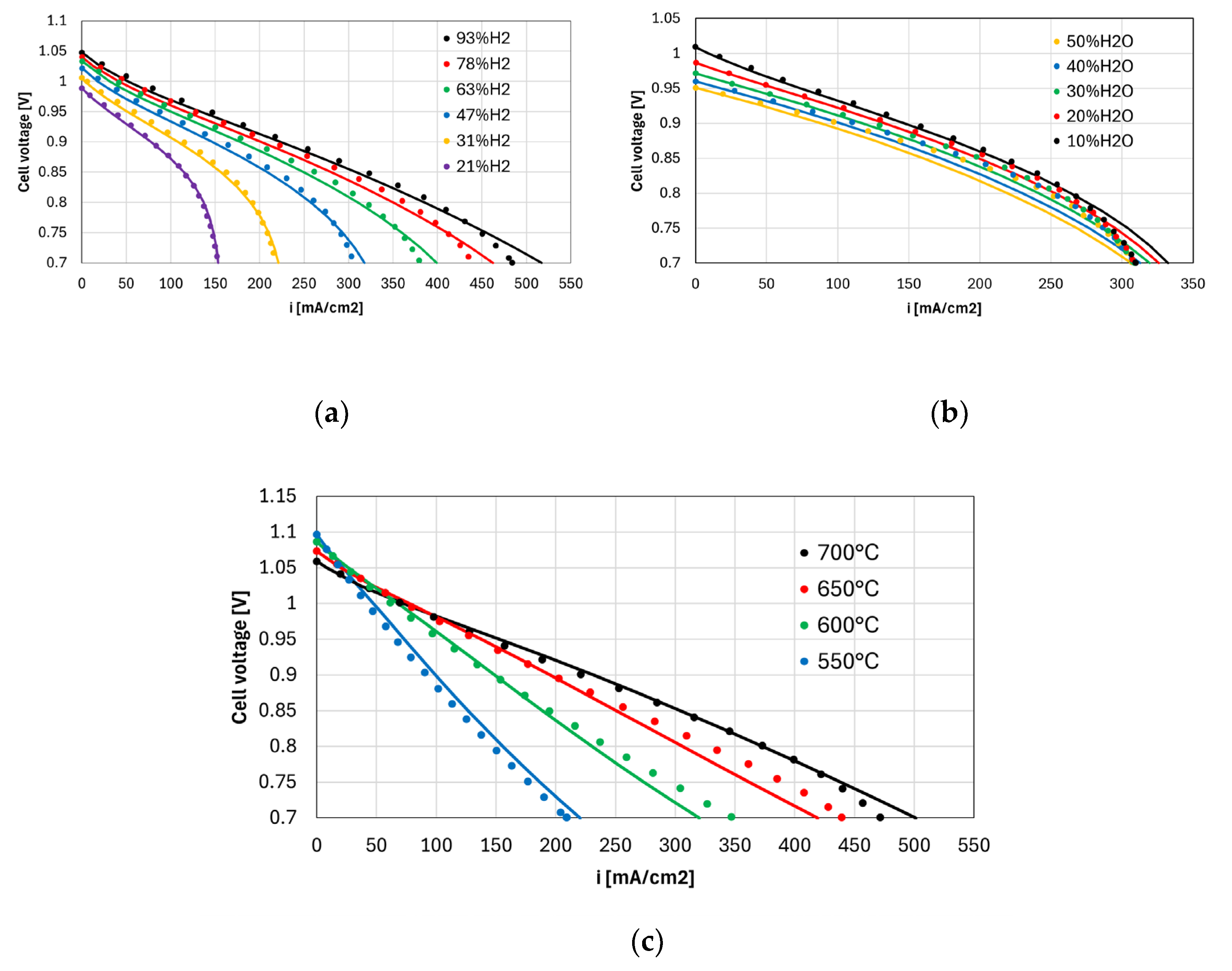
Figure 5.
Figure 5. Polarization losses calculated in selected operating conditions: (a) 7% H2O and 21% H2 (N2 balance) at 750 °C, (b) 50% H2 and 50% H2O at 750 °C, (c) 7% humidified H2 at 550 °C.
Figure 5.
Figure 5. Polarization losses calculated in selected operating conditions: (a) 7% H2O and 21% H2 (N2 balance) at 750 °C, (b) 50% H2 and 50% H2O at 750 °C, (c) 7% humidified H2 at 550 °C.
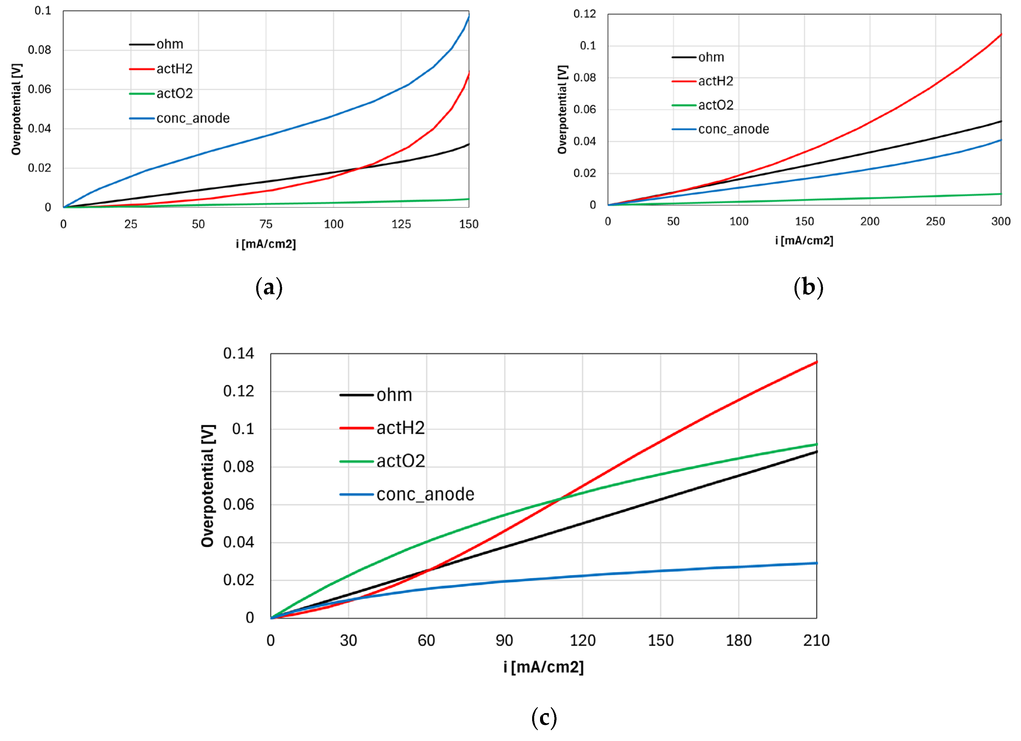
Figure 6.
Figure 6. Results of the adiabatic simulation: (a) temperature distribution of PEN, interconnects, and gas streams, (b) current density profile, (c) fuel stream composition along the channel, (d) effect of grid refinement on PEN temperature distribution.
Figure 6.
Figure 6. Results of the adiabatic simulation: (a) temperature distribution of PEN, interconnects, and gas streams, (b) current density profile, (c) fuel stream composition along the channel, (d) effect of grid refinement on PEN temperature distribution.
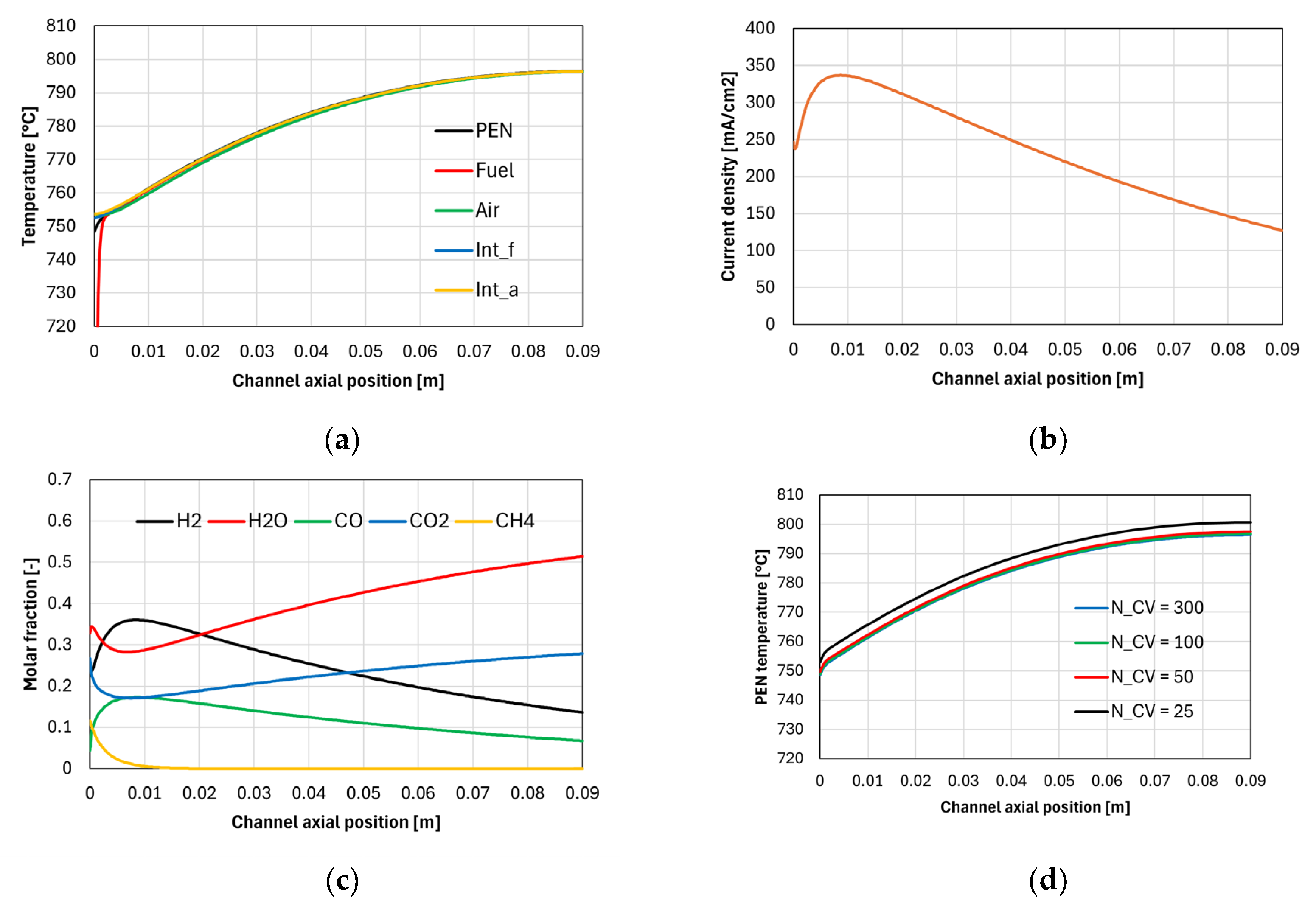

Table 1.
elevant geometrical parameters derived from the input channel geometry.
| Symbol | Equation | Description |
| Active area per unit length | ||
| PEN thickness | ||
| Cross-sectional area of the interconnect | ||
| Cross-sectional area of the fuel electrode | ||
| Cross-sectional area of the air electrode | ||
| Cross-sectional area of the electrolyte | ||
| Cross-sectional area of the PEN assembly |
Table 2.
Summary of heat and enthalpy exchanges between gas and solid parts.
| PEN | Interconnect (fuel and/or air side) | |
| Gas channel (fuel or air) |
||
| PEN | - |
1 is the enthalpy of the pure species calculated with the local PEN or gas temperature in case is positive or negative, respectively.
Table 3.
Input parameters used for the model validation.
| Parameter | Value | Source |
| Channel | ||
| 4 cm | [4] | |
| 2 mm | [4] | |
| 2 mm | [4] | |
| 1 mm | [4] | |
| 1 mm | [4] | |
| 1.6 cm2 | ||
| 5.486 Nml min-1 cm-2 | fitted | |
| 93.75 Nml min-1 cm-2 | [4] | |
| 100 | ||
| Fuel electrode | ||
| 400 μm | [4] | |
| 0.28 | [4] | |
| 7.5 | fitted | |
| 0.16 μm | [4] | |
| 100 kJ mol-1 | fitted | |
| 3.2 x 10⁸ A m-2 | fitted | |
| 0.5 | fitted | |
| -1 | fitted | |
| 0.5 | [4] | |
| Air electrode | ||
| 15 μm | [4] | |
| 0.2 | [4] | |
| 3.0 | [4] | |
| 0.25 μm | [4] | |
| 135.0 kJ mol-1 | fitted | |
| 2.2 x 10¹¹ A m-2 | fitted | |
| 0.22 | [4] | |
| 0.65 | [4] | |
| Electrolyte | ||
| 3.1 μm | [4] | |
| 61.1 kJ mol-1 | fitted from EIS [4] | |
| 1 | 261945 S K m-1 | fitted from EIS [4] |
| 0.0 |
1 This value is valid for experiments with varying and performed at 750 °C. For experiments at 700 °C, 650 °C, 600 °C, and 550 °C, 464167 S K m-1.
Table 4.
Operating conditions of the SOFC in the hybrid system with a bottoming steam cycle [2].
Table 4.
Operating conditions of the SOFC in the hybrid system with a bottoming steam cycle [2].
| Parameter | Value | Description |
| General | ||
| 0.8 V | Cell voltage | |
| 66.4% | Single-pass H2 utilization factor | |
| Heat loss | 2% | Heat loss (fraction of fuel LHV) |
| 800 °C | Outlet cell temperature | |
| Fuel inlet | ||
| 521 °C | Inlet fuel temperature | |
| 1.15 bar | Inlet fuel pressure | |
| 24.16% | Inlet H2 fraction | |
| 32.83% | Inlet H2O fraction | |
| 4.45% | Inlet CO fraction | |
| 26.66% | Inlet CO2 fraction | |
| 11.55% | Inlet CH4 fraction | |
| 0.35% | Inlet N2 fraction | |
| Air inlet | ||
| 754 °C | Inlet air temperature | |
| 1.15 bar | Inlet air pressure | |
| 20.73% | Inlet O2 fraction | |
| 77.28% | Inlet N2 fraction | |
| 1.03% | Inlet H2O fraction | |
| 0.96% | Inlet Ar fraction |
1 Reference [2] shows 0.86 V, but this value is too large to guarantee a significant current density near the channel exit.
Disclaimer/Publisher’s Note: The statements, opinions and data contained in all publications are solely those of the individual author(s) and contributor(s) and not of MDPI and/or the editor(s). MDPI and/or the editor(s) disclaim responsibility for any injury to people or property resulting from any ideas, methods, instructions or products referred to in the content. |
© 2026 by the authors. Licensee MDPI, Basel, Switzerland. This article is an open access article distributed under the terms and conditions of the Creative Commons Attribution (CC BY) license (http://creativecommons.org/licenses/by/4.0/).
Copyright: This open access article is published under a Creative Commons CC BY 4.0 license, which permit the free download, distribution, and reuse, provided that the author and preprint are cited in any reuse.


