1. Introduction
The collective motion of animal swarms, flocks, and schools has fascinated researchers since the earliest systematic observations of natural behavior. Only in the past two decades, however, has this interest extended beyond biology and ethology to disciplines such as robotics and computer science. It has been widely observed that natural swarms are capable of complex cooperative behaviors (including obstacle avoidance, collective defense, and efficient resource gathering) without relying on centralized coordination or leadership. Such systems exhibit remarkable robustness, as their homogeneous structure ensures that no individual agent represents a single point of failure. Inspired by these properties, swarm-based paradigms have been extensively investigated in robotics [
1,
2,
3,
4], and more recently have attracted growing attention within the space community as well [
5,
6]. Future space missions may involve large groups of small autonomous agents, such as cooperative flying robots for planetary exploration, swarms of probes for asteroid belt reconnaissance, or distributed formations in low Earth orbit (LEO) for remote sensing applications [
7,
8]. The authors have previously explored the application of swarming concepts to spacecraft systems for tasks such as autonomous self-assembly and orbital migration [
9,
10].
A foundational contribution to swarm modeling was introduced by Reynolds [
11], who proposed three heuristic interaction rules to reproduce collective behavior: cohesion (attraction toward neighboring agents), alignment (velocity matching), and separation (collision avoidance). One of the central challenges in swarm control design lies in providing rigorous stability guarantees for such decentralized systems. In this context, Olfati-Saber [
12] developed a theoretical framework for distributed flocking algorithms that incorporate all three of Reynolds’ principles and yield structured quasi-crystalline formations.
The implementation of these simple interaction laws depends strongly on the operating environment. In this work, their application is investigated in the context of spacecraft formations. Specifically, the focus is on large swarms of microsatellites tasked with maintaining a cohesive formation while ensuring collision safety. Related work addressing decentralized drift mitigation under communication constraints can be found in [
13], where only satellites within a limited communication region participate in relative motion estimation. However, that study does not explicitly consider collision avoidance nor the impact of relative navigation uncertainties.
In the present study, ground intervention is assumed to be unavailable and onboard computational resources are considered severely constrained. The objective is therefore to achieve autonomous swarm maintenance using only minimal onboard sensing, provided by a single monocular camera. As explained in [
14], different missions were conducted focusing on angles-only navigation, such as AVANTI [
15] and ARGON [
16], focused primarily on relative state estimation and relied on external absolute orbit knowledge (e.g., GNSS measurements) to guarantee convergence. More recently, the Starling Formation-flying Optical eXperiment (StarFOX) has aimed to overcome these limitations by implementing a fully autonomous angles-only absolute and relative trajectory measurement system.
In contrast to these approaches, behavioral strategies do not require explicit target identification, as all swarm agents are considered equivalent. Although each spacecraft observes only a small subset of the swarm at any given time, an appropriately designed behavioral guidance law enables autonomous and fuel-efficient swarm maintenance while preserving collision safety. Particular emphasis is placed on the role of relative navigation accuracy, which directly affects guidance quality and control effort.
The remainder of this paper is organized as follows.
Section 2 introduces the orbital dynamics models employed in the study.
Section 3 describes the mission scenario and the adaptation of the behavioral laws to the space environment.
Section 4 presents simulation results assuming ideal relative-state knowledge, while
Section 5 investigates the impact of navigation uncertainties associated with a rough vision-based estimation scheme. Finally, conclusions are drawn in
Section 6.
2. Relative orbital dynamics: hypothesis and models
A detailed and long-term evaluation of the control performance of a swarm of satellites require the development of a high precision orbital propagator (HPOP), including at least the first zonal harmonics of the Earth potential and a model of the atmosphere with time varying density. However, the nature of this study is purely qualitative, with the task of showing the feasibility and limitations of the behavioural control; therefore, a HPOP would just slow-down the simulation time without changing the general conclusions. The relative motion of the satellites is computed by using a simplified model, illustrated for example in [
17], which is a linear model able to include the effects of J2 and drag perturbation in quite an easy and straight forward way. According to this model, the relative motion is described by a vector of differential mean orbital elements:
With
where subscript
T and
C stand for Target (the reference satellite) and Chaser, respectively;
a is the mean semimajor axis,
e the mean eccentricity
, i the mean inclination,
the mean argument of perigee, Ω the mean Right Ascension of the Ascending Node (RAAN),
u the mean argument of latitude. It must be noted that in the case of swarms, there is not a real Target satellite: the group is composed by homogeneous satellites with no special roles, so Target just indicates the satellite that at a given time is taken as reference.
For the case of interest (nearly circular orbits), the dynamics follows a simple linear propagation law:
Where
are the control accelerations in a LVLH frame. The state matrix
A(t) can contain both the gravity gradient effects (i.e. the equivalent of the classic HCW dynamics) and J2 gradient effects, depending of course on the chief orbital elements. Atmospheric drag effects can also be easily added by increasing the state vector and including the variation of the semimajor axis. Description of the matrix can be found in [
17]. For the sake of simplicity, due to the very qualitative and high-level nature of the study, only Keplerian forces are here considered. The input matrix
B reads as:
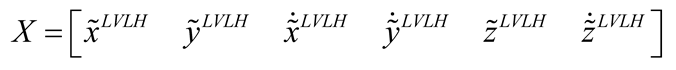
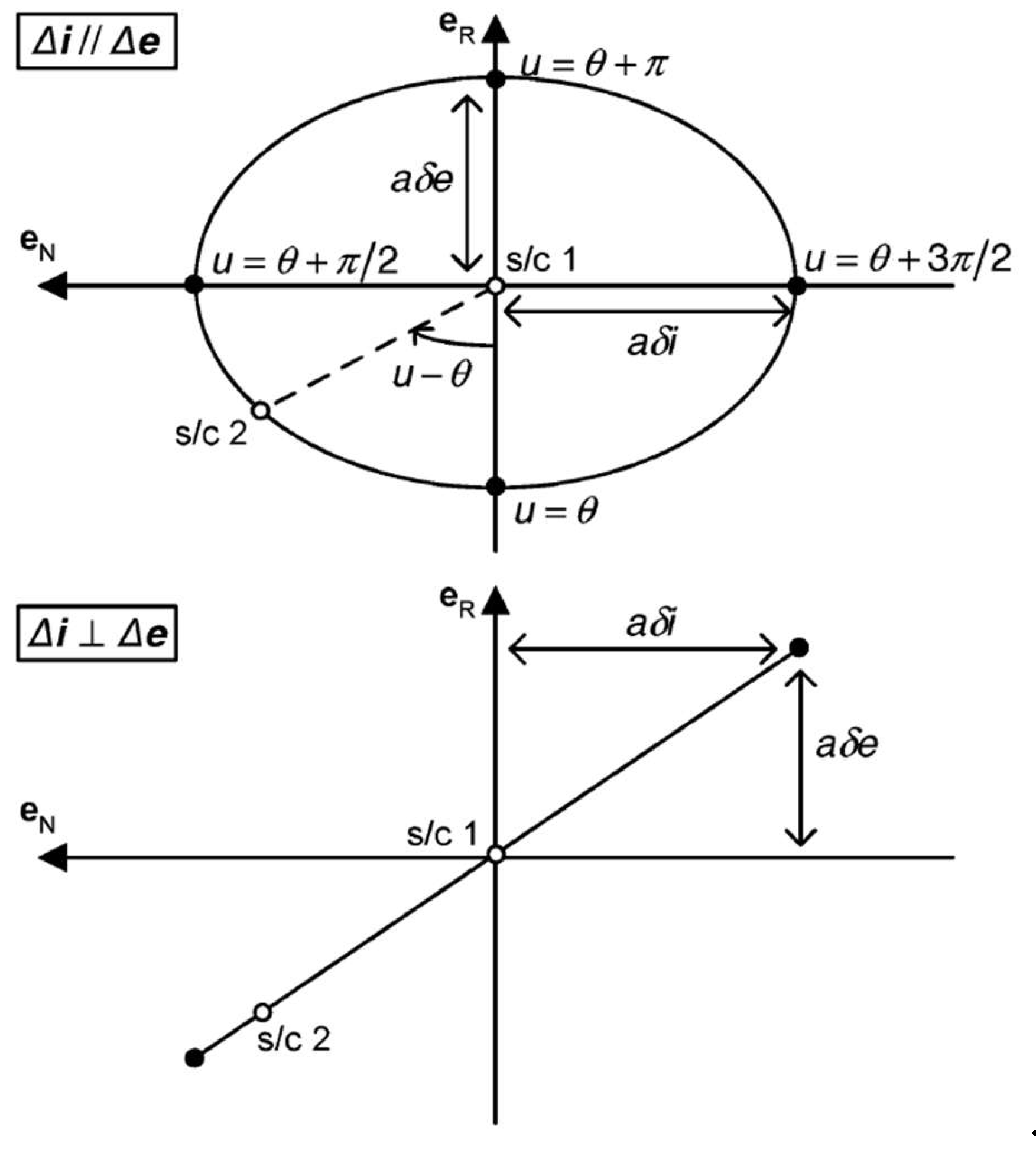
Even though relative coordinates in the Local Vertical Local Horizontal (LVLH) frame are maybe easier and more immediate to interpret – and in fact they will be used in the following to plot the relative trajectories, with x being the radial direction, z the out-of-plane trajectory and y forming a right-handed frame), the physical meaning of the differential mean orbital elements has been also clearly explained (for example in [
18]), and briefly pictured in
Figure 1.
The differential semimajor axis is of course connected to a drift in the formation; differential eccentricity and differential inclination are connected to the in-plane and out-of-plane dimension of the relative motion ellipse.
3. Behavioural laws in a space scenario
In this paper, we will try to adapt the general behavioural laws to the space scenario, with its peculiar limitations (in particular, in the satellite maneuvering capabilities) and in the environmental forces.
3.1. The mission scenario
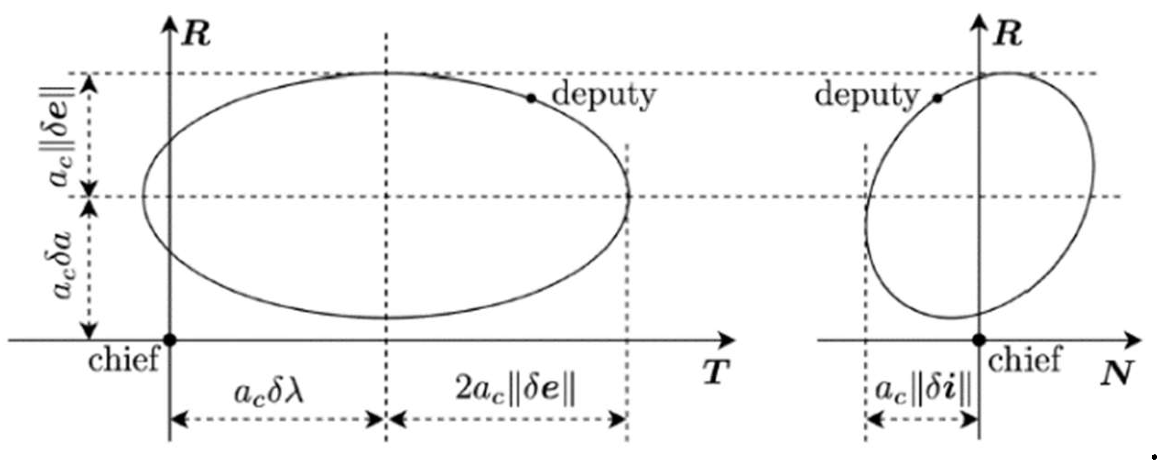
The mission scenario considered in this study consists of a fleet, or swarm, of spacecraft acting as autonomous agents. Each spacecraft is equipped with a single monocular camera rigidly aligned with the along-track direction. The sensor features a 60° field of view (FOV) and a resolution such that targets located beyond 500 m cannot be reliably detected.
As introduced earlier, the behavioral control framework is based on three elementary interaction rules: repulsion from nearby neighbors to ensure collision avoidance, attraction toward distant neighbors to preserve cohesion, and alignment with agents at intermediate range to regulate the overall formation geometry. The control input applied by each
j-th agent is obtained by superimposing the contributions computed with respect to all visible
k-th agents. Only spacecraft lying within the sensor FOV and detection range are considered in the control process. The implications of partial knowledge of the swarm state have been investigated, for instance, in [
19]. As shown in
Figure 2, in the proposed space scenario another spacecraft can be detected only if it is inside the FOV, at a distance less than the maximum possible for the sensor characteristics (therefore, considering
Figure 2, only spacecraft A and B are detected and contributes to the computation of the control action).
3.2. Definition of the threshold distances
When designing the control actions, not only swarm cohesion (i.e., prevention of relative drift) and safety (i.e., collision avoidance) must be ensured, but also persistent mutual visibility. Accordingly, three key distance parameters are introduced:
: minimum distance in the radial or out-of-plane direction (for collision avoidance issues);
: minimum distance in the along-track direction (for collision avoidance issues);
: maximum distance to detect another spacecraft (for visibility issues).
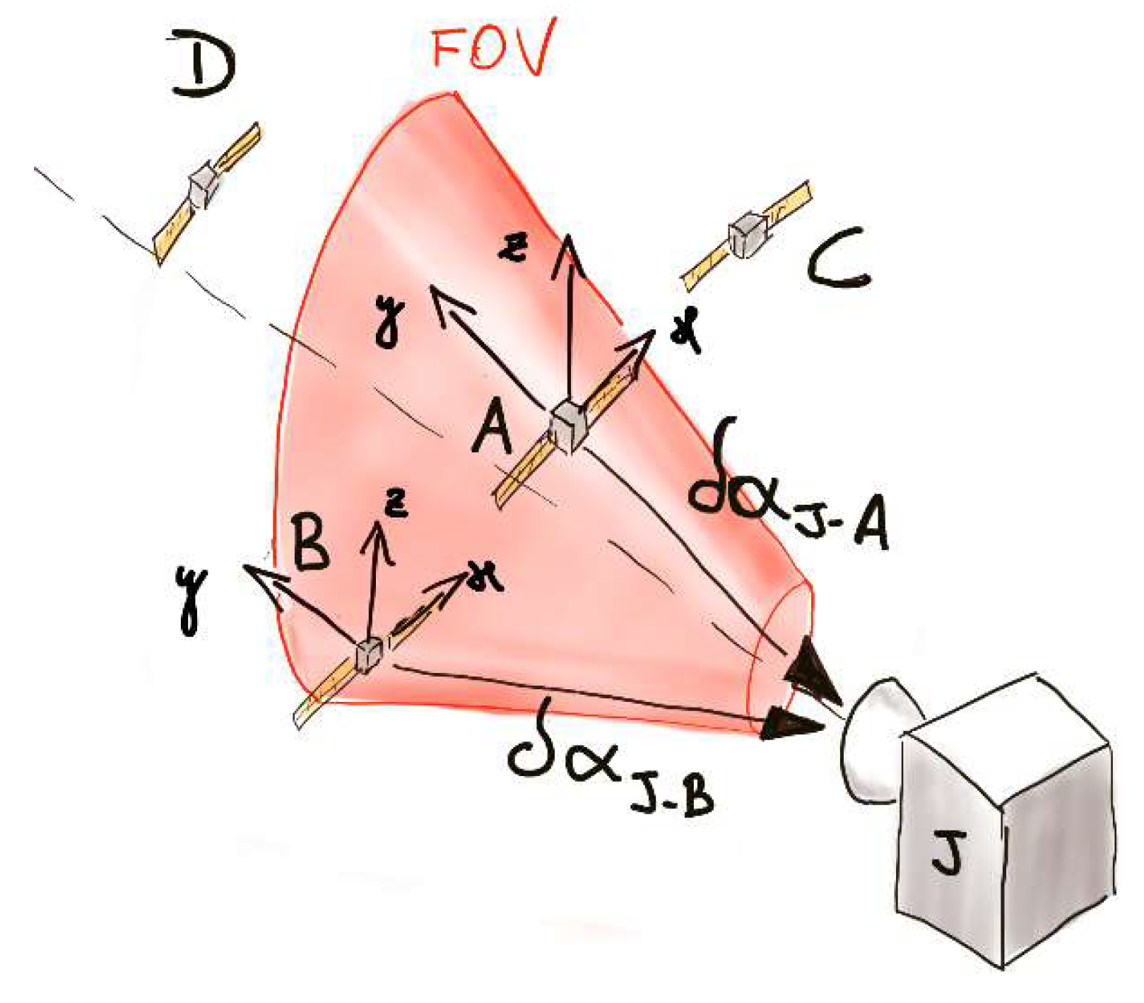
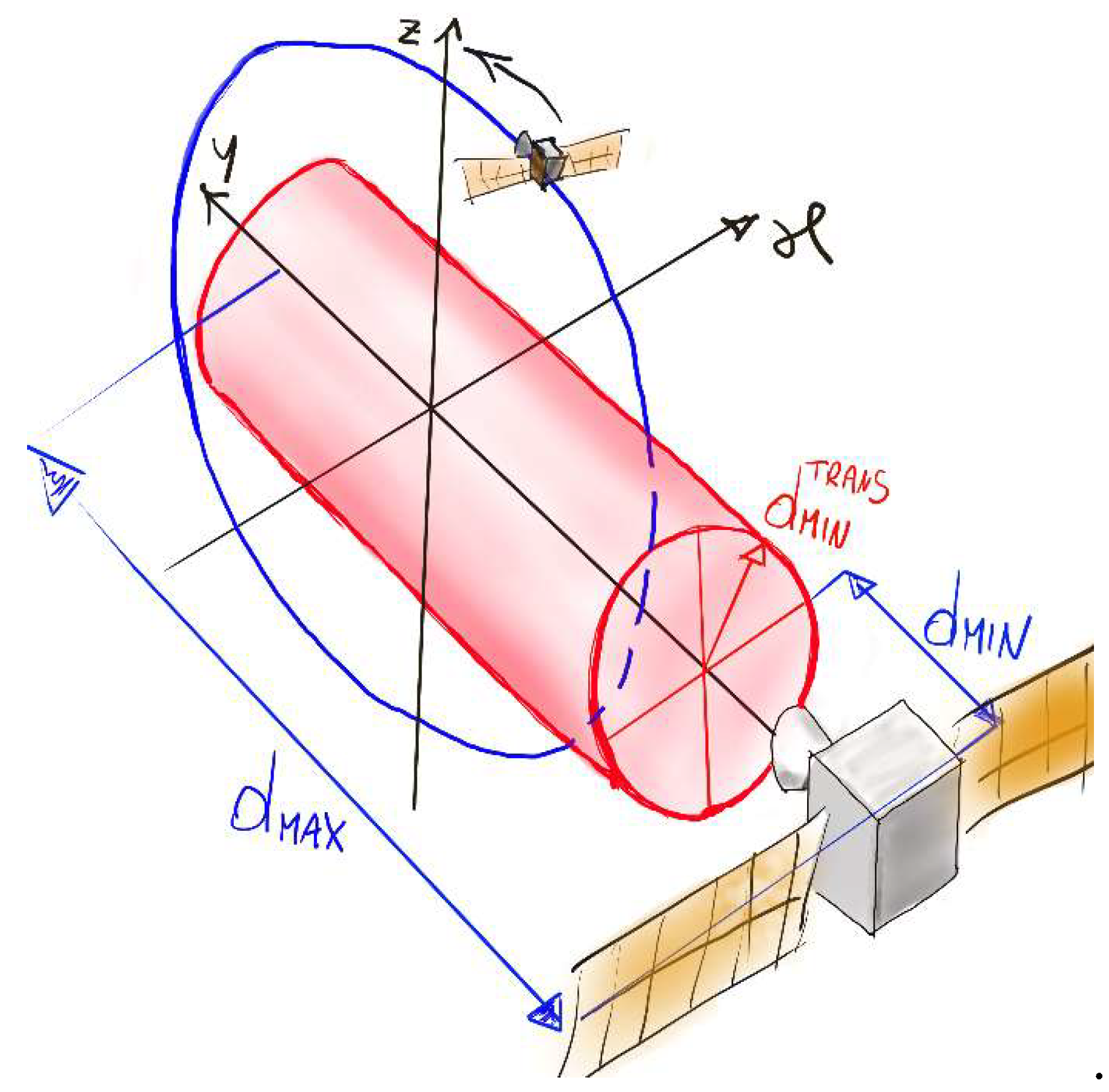
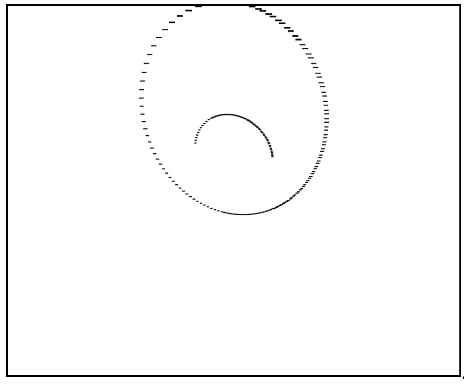
Within this framework, the ideal relative trajectory of a satellite
k-th with respect to a satellite
j-th is the one depicted in
Figure 3. The desired motion is a bounded, periodic relative ellipse with no secular drift, confined between prescribed minimum and maximum separations. Moreover, the cross-track and out-of-plane components are shaped so as to avoid interception of the along-track axis, thereby providing an additional safety margin: in the event of a failure, the resulting relative drift would not lead to a collision. While such configurations may result in locally dense regions within large swarms, the role of the behavioral control laws is precisely to establish and maintain a globally stable and safe configuration through purely decentralized decision-making.
In order to achieve this behavior, the regions and the respective actions of attraction, alignment and repulsion must be carefully defined.
3.3. Definition of the decision distances
The selection of the appropriate control action among repulsion, alignment, and attraction is governed by the intersatellite separation. A straightforward choice would be to define this distance as the Euclidean norm of the relative position vector. However, both the in-plane and out-of-plane components of the relative motion exhibit periodic behavior, which may lead to correct decisions being triggered at inappropriate times. For instance, a satellite may be dangerously close when it lies outside the field of view, or it may appear to be at a safe distance at a given instant while approaching a critical configuration within less than one orbital period.
For this reason, the decision metric is not based solely on instantaneous relative distance, but instead relies on the mean differential orbital elements. These parameters capture the geometry and long-term evolution of the relative trajectory, thereby enabling predictive decision-making and allowing corrective actions to be initiated before unsafe or undesirable configurations develop.
At each decision sample time (not necessarily short: 10 seconds between two successive measurements is selected for the following simulations) the j-th satellite detects a certain number of k-th satellite, places a reference upon each of them and finally it computes the relative state . The navigation issue is for the moment skipped and we suppose perfect knowledge the vector.
In a stationary condition, the differential semimajor axis will be small; the shape of the relative trajectory is a walking ellipse with limited drift. Upon an orbital period, it is meaningful to consider that the minimum relative distances will be determined by (see
Figure 1):
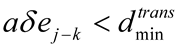
The repulsion, or collision avoidance (CA), area will be entered if . The attraction area will be entered if . The alignment zone is in between.
3.4. Control laws
The selection of the control algorithm of course affects the performance of the behavioral guidance, but it is not the core objective of the present research. A Linear Quadratic Regulator [
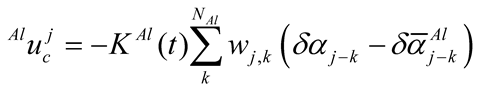
20] based on the linear dynamics equations (2) is used. Since the state matrix and the input matrix are time-dependent, the Differential Riccati equations must be used instead of usual Algebraic Riccati Equation; this means that the resulting gain are time-dependent as well. The control action, independently from the behavioral law, reads as:
The gain K(t) and the reference state change according to the difference behavioral law. The error with respect to the reference state is summed up over all Nvis visible satellites, and can be weighted according to the relative distance (see paragraphs 3.5, 3.6, 3.7).
3.5. Collision avoidance algorithm
When the j-th agent is too close with respect to a k-th agent, it is considered a very dangerous situation, and therefore the objective is to perform a fast maneuver for increasing the relative distance and guiding the satellites to a safe configuration.
It has been shown in [
21] that parallel differential eccentricity and inclination vectors offers maximum safety with respect to collision avoidance; in fact, a failure of one satellite with consequent along-track drift would not lead to a collision, as shown in
Figure 4.
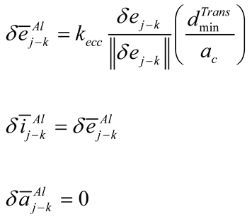
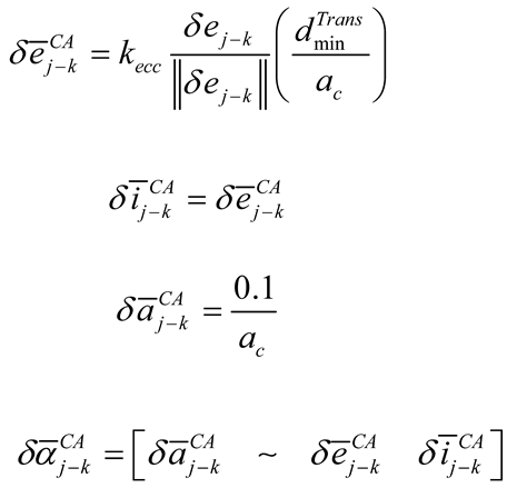
The desired relative state is specified by assigning a differential eccentricity vector that preserves the direction of its current value while increasing its magnitude to a level exceeding the minimum allowable threshold
by a prescribed factor
(set to
in the simulations). The desired differential inclination vector is chosen to be equal to the desired eccentricity vector, thereby enforcing their parallelism. Finally, the desired differential semimajor axis is set to a positive offset of 100 m, which induces a controlled negative along-track drift.
The control weight matrix of the LQR, is set to R = 104I3x3 a value which, as shown in the next paragraphs, is one or two orders of magnitude less than in the alignment and attraction cases, leading to a much larger control action.
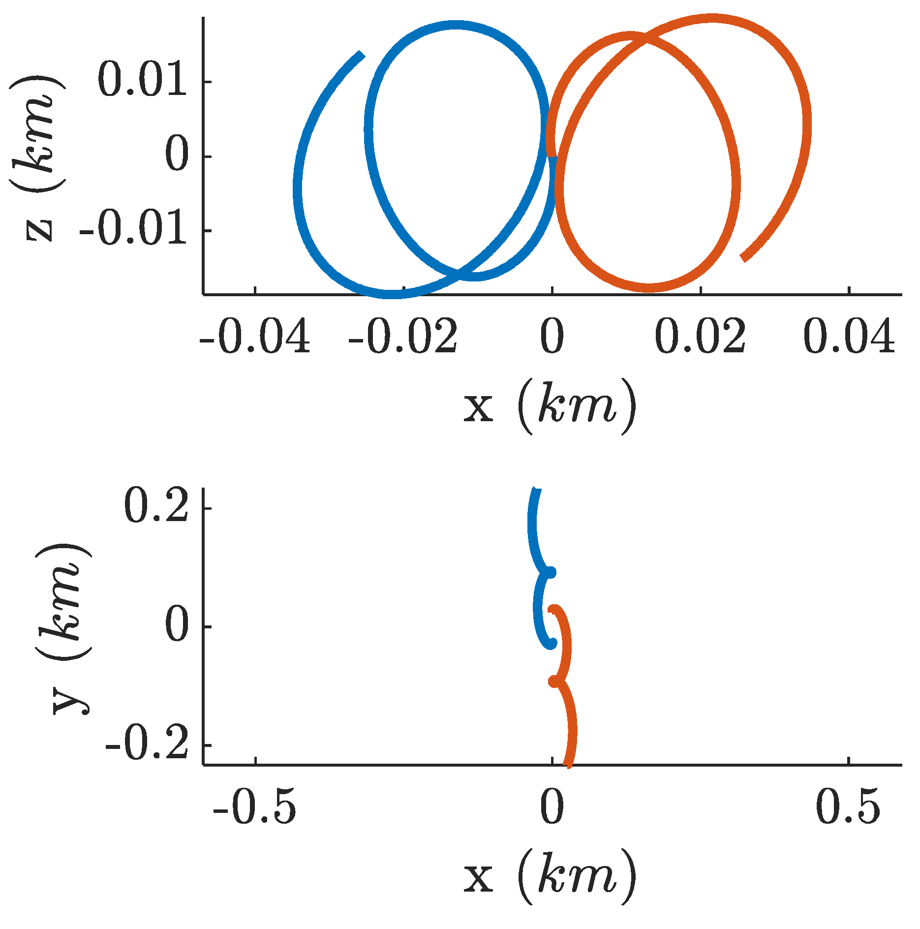
As an initial validation of the collision-avoidance (CA) maneuver, a simplified scenario involving only two satellites is considered. The initial conditions are selected such that the follower satellite detects a neighboring agent at an unsafe distance and consequently activates the CA control law, while the alignment and attraction behaviors are temporarily disabled. As shown in
Figure 5, the along-track separation between the two spacecraft is successfully increased to a safe value. The apparent motion of both satellites is a consequence of expressing the relative trajectories in a reference frame centered at the swarm center of mass, which is adopted here and throughout the remainder of the paper.
In the collision-avoidance regime, no weighting is applied to the tracking error between the relative state vector and the corresponding reference state of the
satellites located within the CA region (
wj,k = 1).
3.6. Alignment algorithm
Within the alignment region, the primary objectives are to suppress relative drift and to maintain a cross-track separation that is sufficiently large to ensure collision avoidance, yet small enough to guarantee persistent mutual visibility.
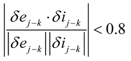
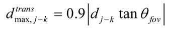
Table 1 reports the main steps of the algorithm. First the dimension of the cross-track relative trajectory is evaluated, and compared both to
(to check if the dimension is too small) and to
, a maximum transverse dimension that is computed to preserve the k-th satellite inside the FOV (specifically, 90% of the maximum transverse distance to be inside the FOV). Finally, the parallelism between the differential eccentricity and differential inclination is checked. If one of the three conditions is met (
TooSmall,
TooLarge,
NotParallel) the alignment control action
is computed.
At the scope, the relative desired state is defined similarly to the collision avoidance case, with the difference that desired differential semimajor axis is zero.
In the alignment regime, the tracking error is weighted so as to assign greater importance to the closest neighboring agents; the weight parameter wj,k scales linearly from 1 when to 0 when dmin = 0.6LMAX (a the borders of the alignment region). The gain KAL(t) is computed with a control weight matrix R = 106I3X3. NAl is the number of satellites in the alignment area of the j-th satellite.
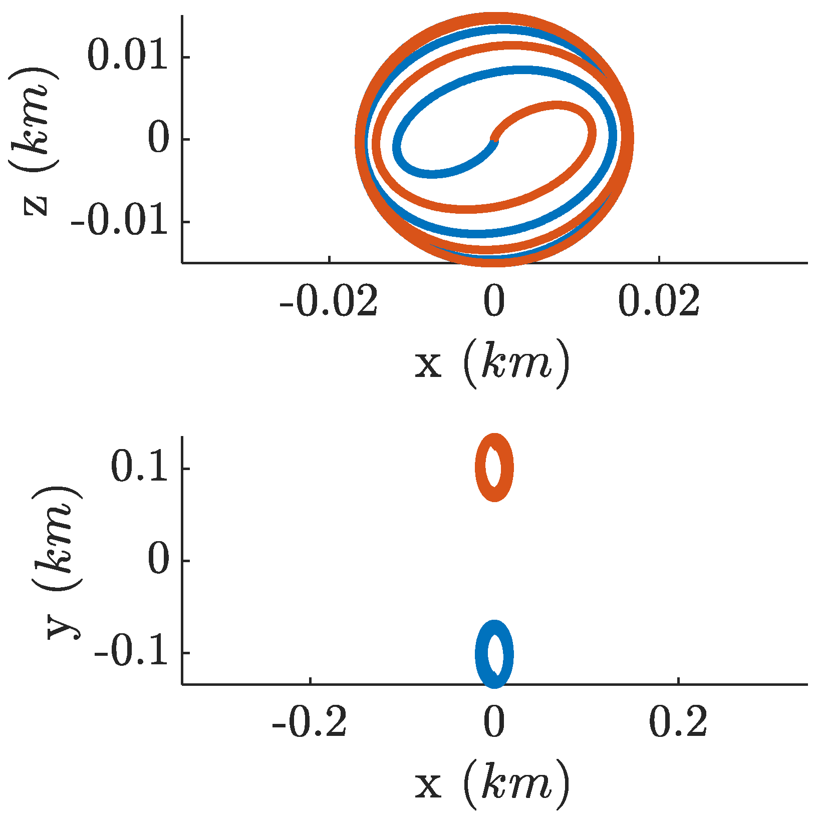
To validate the correctness of the alignment algorithm, a simplified two-satellite scenario is considered. The spacecraft are initially separated by a distance that places them within the alignment region, i.e., neither excessively close nor excessively far. However, the initial conditions include a relative drift and an improper transverse separation, characterized by an insufficient cross-track distance and non-parallel differential eccentricity and inclination vectors.
As it is possible to see from
Figure 6, the two satellites move to a safe relative orbit in which the relative motion in the cross-track plane is a circumference and there is a safe along-track separation.
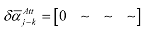
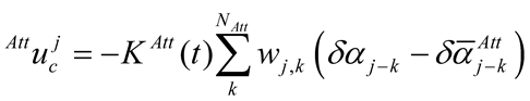
3.7. Attraction algorithm
When the satellite j-th detects a k-th satellite that is still visible but with a range that is so far that it risks exiting the visibility region, the only interest is preventing a further separation. Therefore, the reference state is just set as the differential semimajor axis being zero.
The control gain is computed is computed with a control weight matrix
R = 10
5I3X3.
NAtt is the number of satellites in the attraction area of the j-th satellite. The weighting parameter is
wj,k = 1:
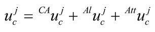
3.8. Control action computation
As mentioned, each j-th satellite computes the actions with respect to all k-th visible satellites, sums them up and applies them.
Unlike the previously considered two-satellite scenarios, each maneuver in a multi-agent swarm is inherently suboptimal with respect to any specific -th neighbor, since each spacecraft simultaneously reacts to multiple agents, each of which is executing its own independent control actions. The resulting collective behavior is therefore uncoordinated, nonlinear, and difficult to predict analytically. Nevertheless, the simulations presented in the following section demonstrate that, under the ideal assumption of perfect relative-state reconstruction, the swarm rapidly converges to a stable and safe configuration in a fully autonomous manner.
4. Simulation set-up
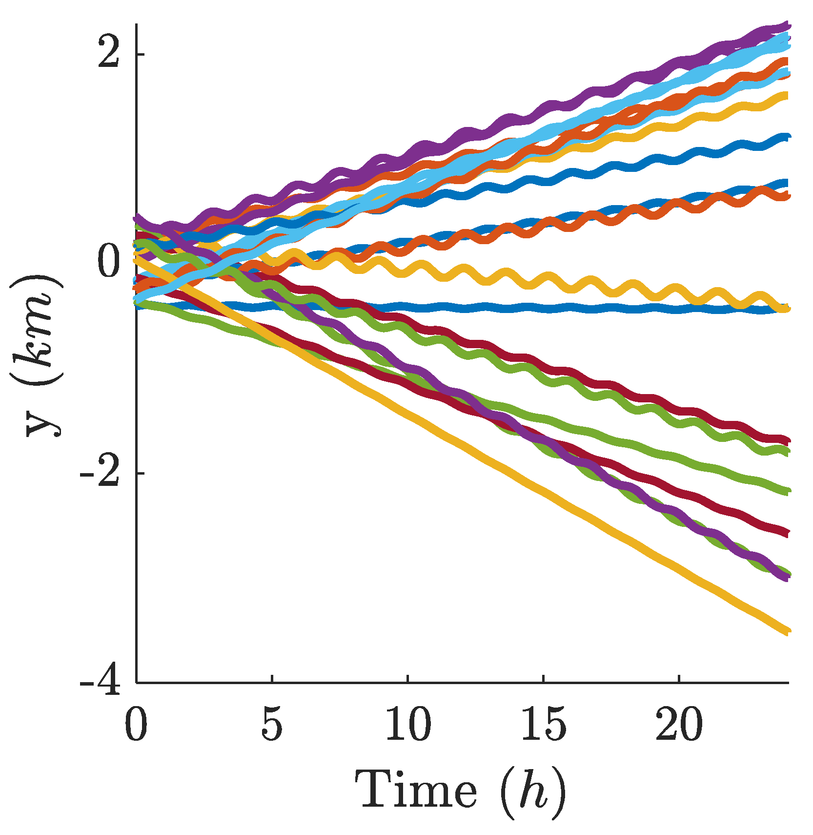
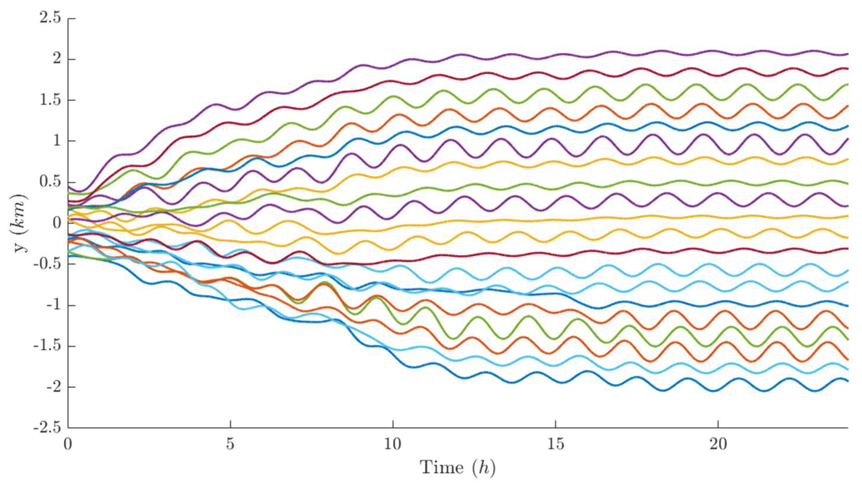
The following simulations consider a swarm composed of 20 spacecraft. The initial conditions are deliberately selected such that, in the absence of control actions, the swarm would rapidly disperse and potentially experience collisions, as illustrated in
Figure 7. It should be noted that the system behavior is highly sensitive to the initial configuration. For instance, if a spacecraft initially neither observes any neighbors nor is observed by others, it will inevitably drift away from the swarm. In behavioral systems, the loss of individual agents may be regarded as an inherent characteristic, since the overarching objective is the survival of the collective rather than that of any single unit. Nevertheless, for space applications, a more conservative approach is adopted here by assuming initial conditions that allow all spacecraft to actively participate in the control process.
Under this assumption, the initial relative orbital elements of the swarm are randomly generated to emulate deployment from a common launch vehicle, with orbital dispersions consistent with the values reported in
Table 2.
4.1. Basics of graph theory
To quantitatively assess the integrity of the swarm, a basic graph-theoretic framework is introduced. A graph is a mathematical structure used to represent pairwise relationships among entities and is composed of vertices (in this case, the satellites) and edges (or links), which indicate that a given -th satellite is visible to a -th satellite. In the present scenario, these relationships are inherently directional: if a -th satellite detects a -th satellite within its field of view, the converse is not true. As a result, the swarm is more appropriately modeled as a directed graph (digraph), in which each edge represents a one-way interaction.
A digraph may be classified as disconnected, strongly connected, or weakly connected. In a strongly connected digraph, every vertex can be reached from any other by following the direction of the edges, whereas in a weakly connected digraph, connectivity is achieved when edge directions are ignored. For the purposes of swarm integrity, weak connectivity is sufficient, as it ensures that every satellite either observes, or is observed by, at least one other member of the swarm.
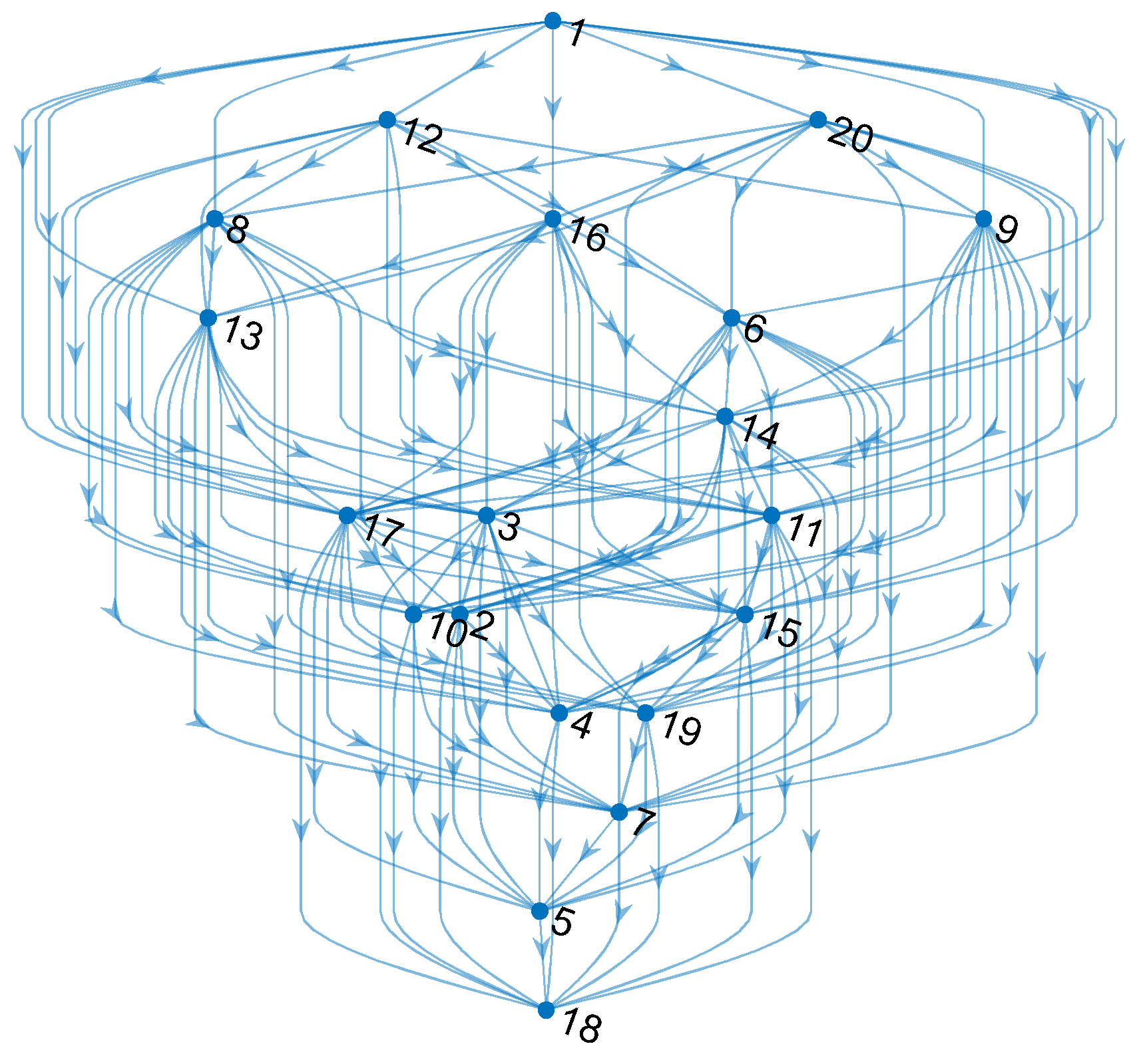
As an illustrative example,
Figure 8 depicts an initial configuration of a 20-spacecraft swarm, where dotted lines indicate visibility links between satellites. In order to determine the integrity of the swarm, the connected components of graph
G are computed as bins (using the MATLAB
conncomp function). For a weakly connected digraph, only one is present, with twenty elements. If more bins are present, it means that the swarm is split in two or more connected subgraphs. The corresponding graph representation at the initial time is shown in
Figure 9, where it can be observed that the swarm is weakly connected, with no isolated nodes. While initial connectivity is necessary, it must be regarded as a dynamic property: a swarm that is initially connected may evolve into a disconnected configuration, either temporarily or permanently. In such cases, the behavioral control laws would fail to preserve swarm integrity.
4.2. Simulation results
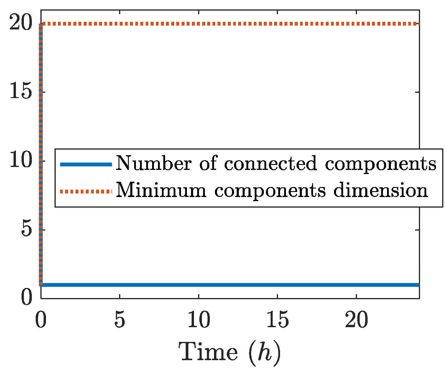
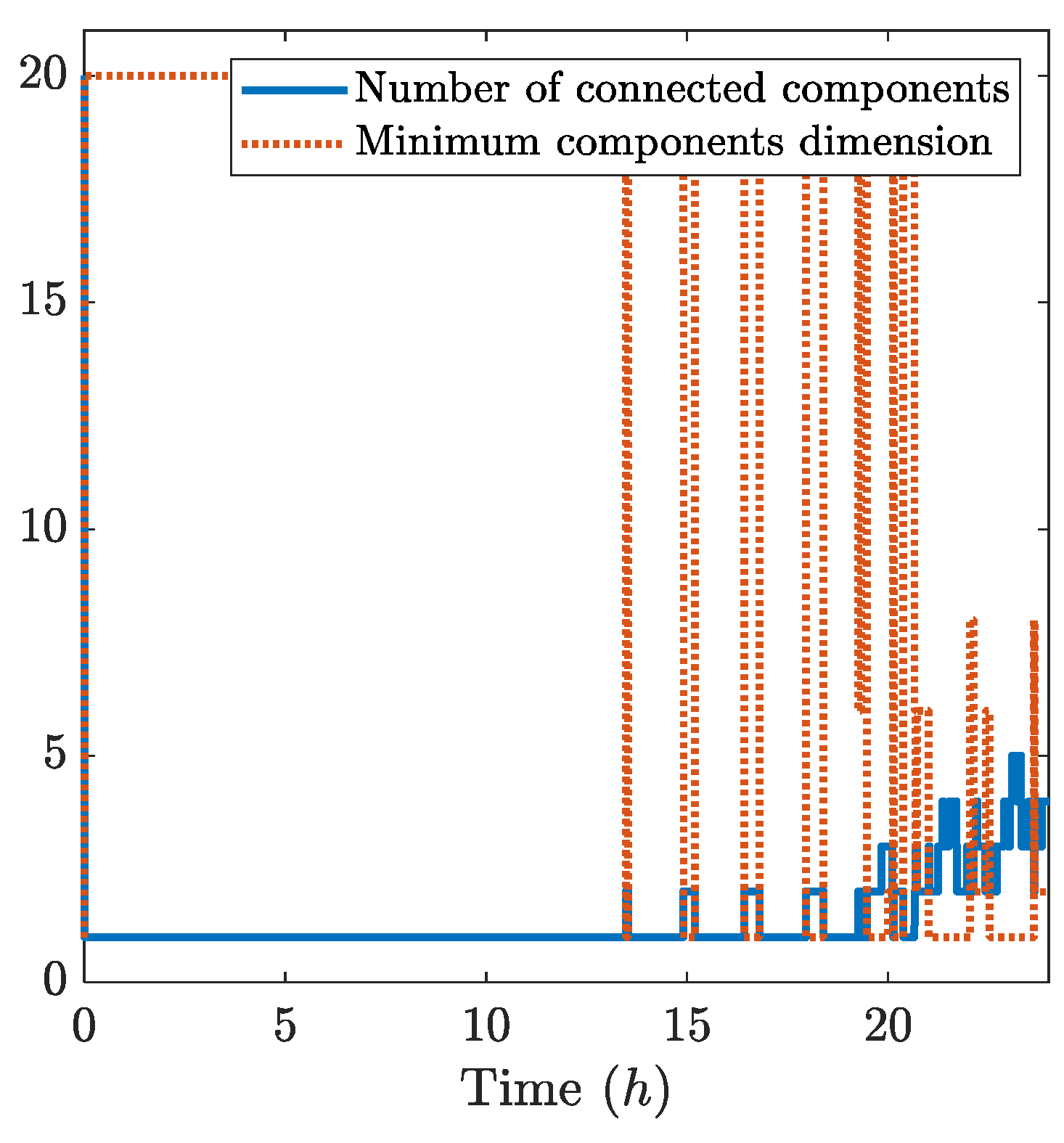
The simulation time is set to 24 hours, and it has been repeated for many different random initial configurations, obtaining (qualitative) similar results: only one sample simulation is here reported for brevity and clarity of the plots. As it is possible to see from
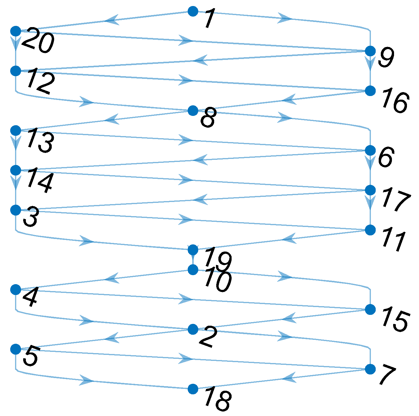
Figure 10, during all simulations there is only one connected component, of course of dimension equal to 20 (i.e., the swarm is always connected). At final time the digraph is represented by
Figure 11, where it is possible to see that no agent is isolated; the only satellite that does not detect other agents is No. 18, which is the spacecraft that preceeds all others.
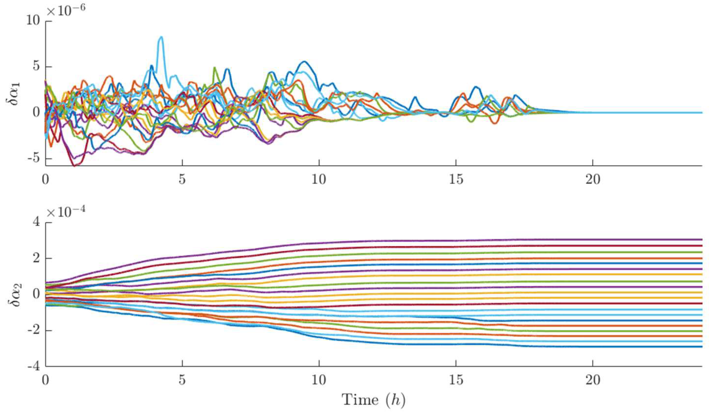
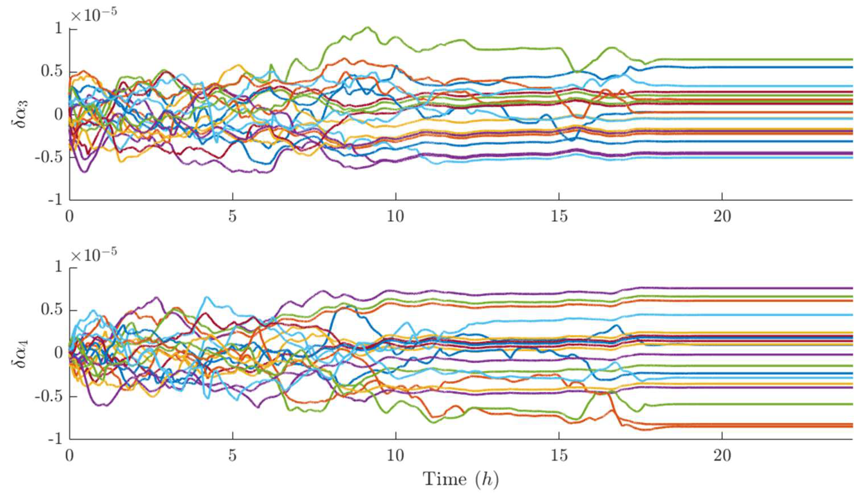
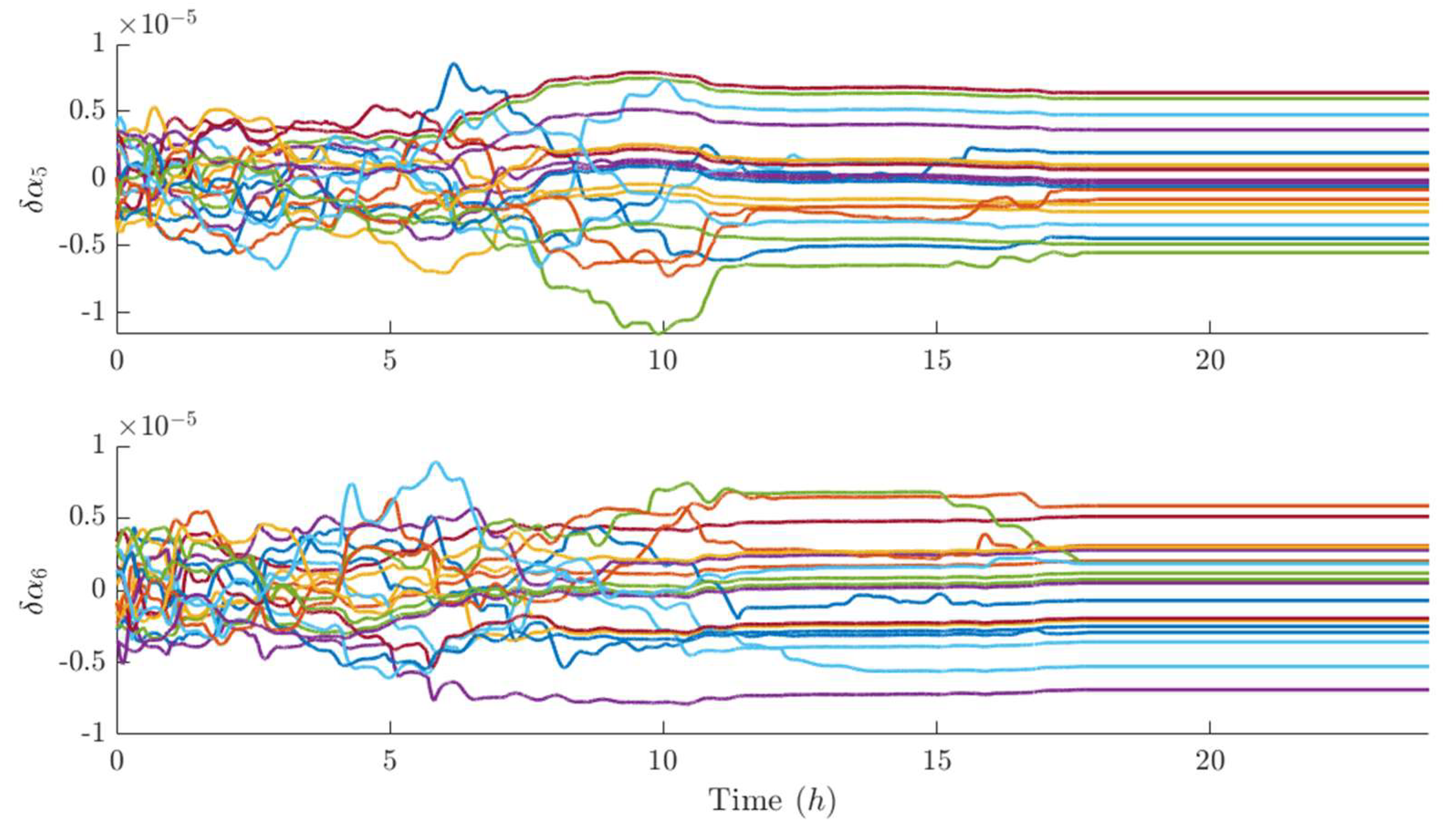
Figure 12,
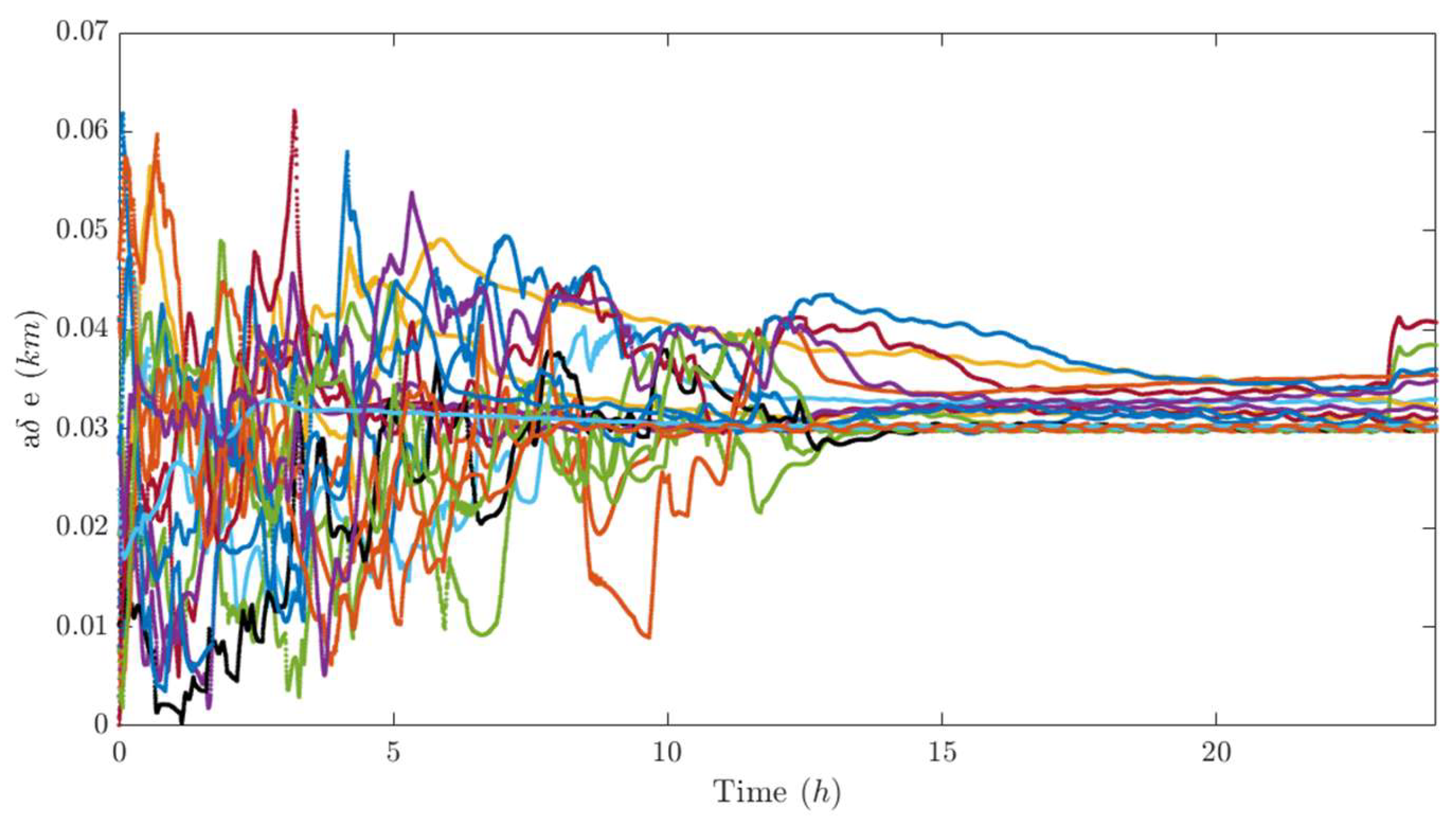
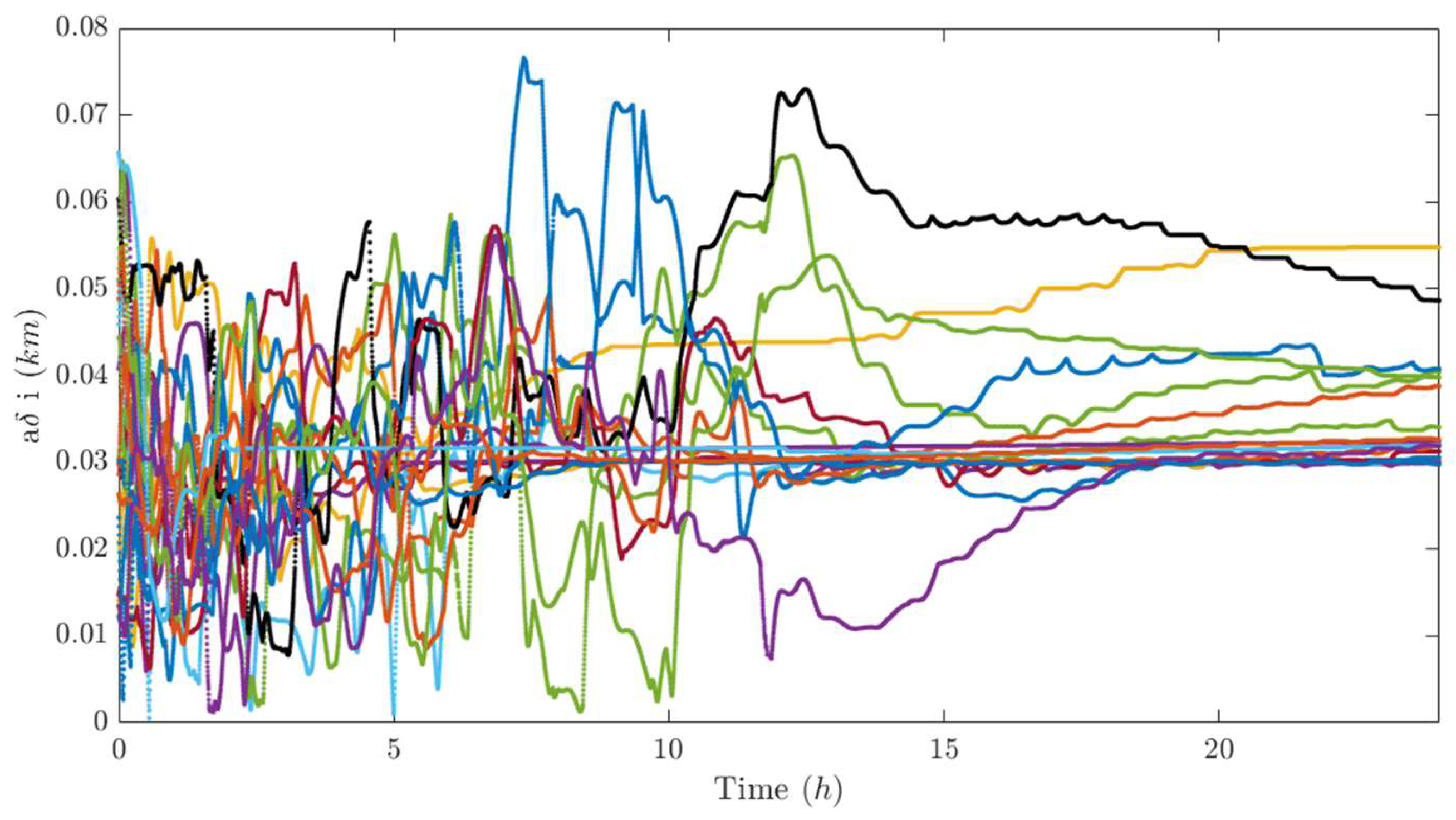
Figure 13 and
Figure 14 reports the components of the differential element vector
δαk of each satellite with respect to the center of mass of the swarm. It can be seen that the differential semimajor axis is set to zero in less than 20 hours (
Figure 12 upper subplot) and the longitudinal separation of the swarm is fairly regular (
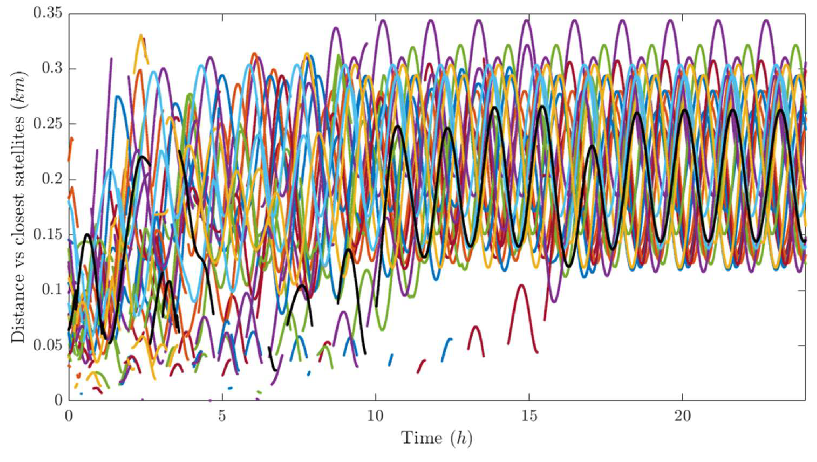
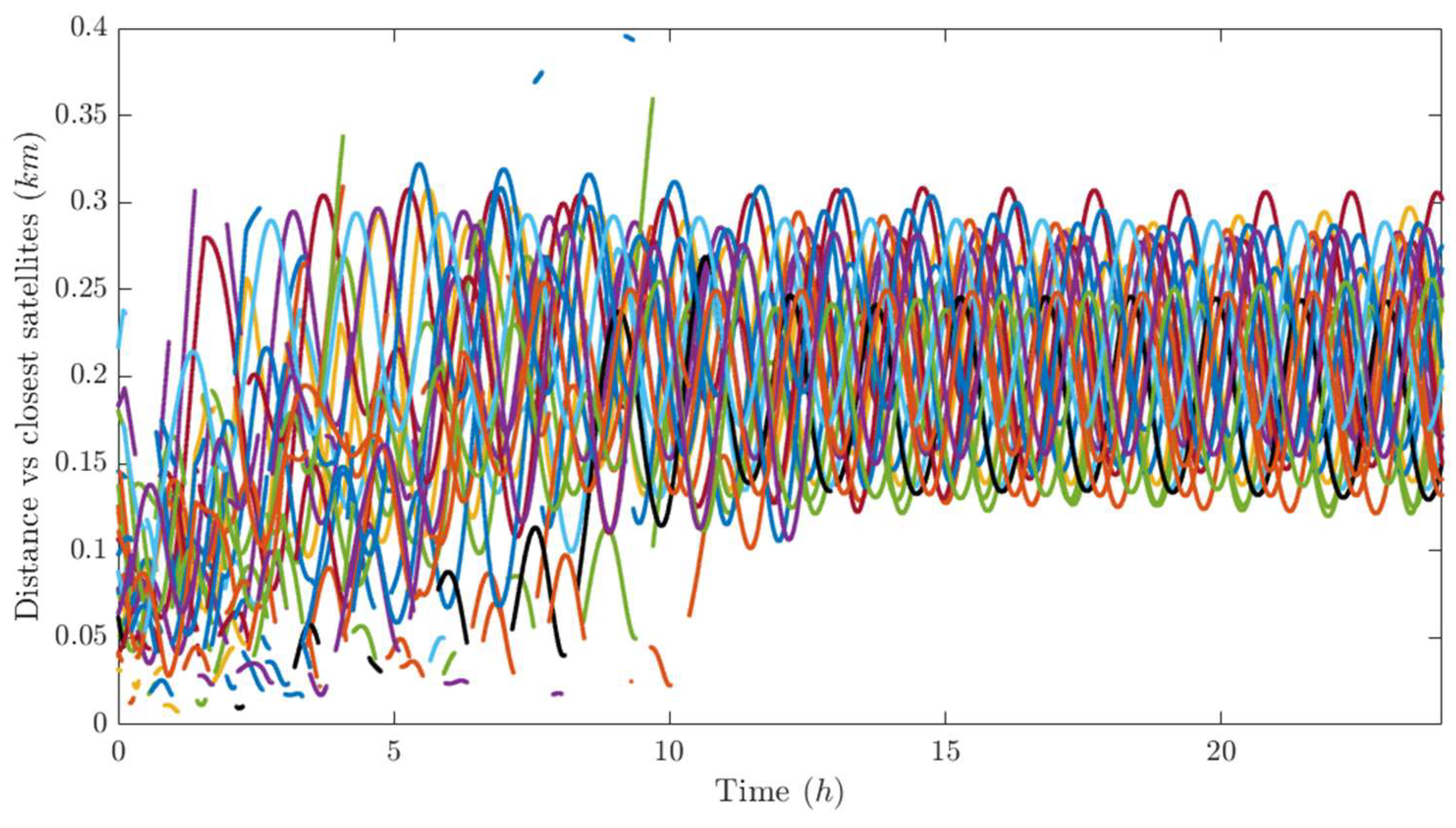
Figure 12 lower subplot). Also, the differential eccentricity and inclination reach a stationary value, which however is difficult to interpret if we do not analyze the performance indices of each j-th satellite with respect to each k-th satellite in visibility. In this sense, the longitudinal distance of each satellite with respect to the closest visible agents is plotted in
Figure 15, and it is greater than the minimum fixed value
dmin at stationary, the out-of-plane and radial dimension of the relative ellipse (
Figure 16 and
Figure 17, respectively) are greater than the minimum transverse distance
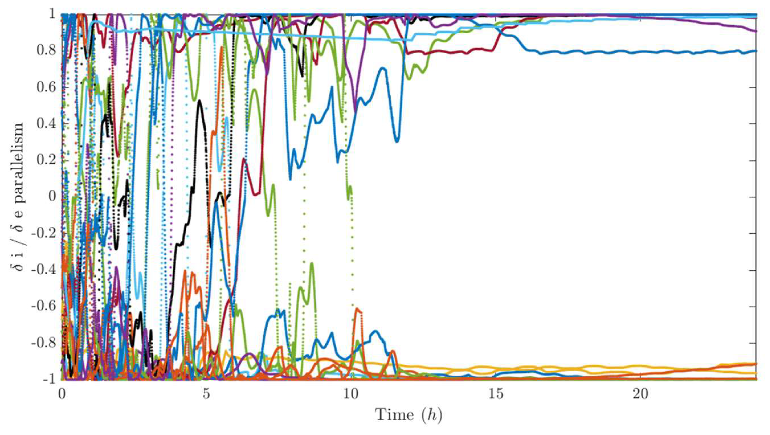
at stationary, and finally the parallelism between relative inclination and relative eccentricity vector is greater (in module) than 0.8 at stationary (
Figure 18).
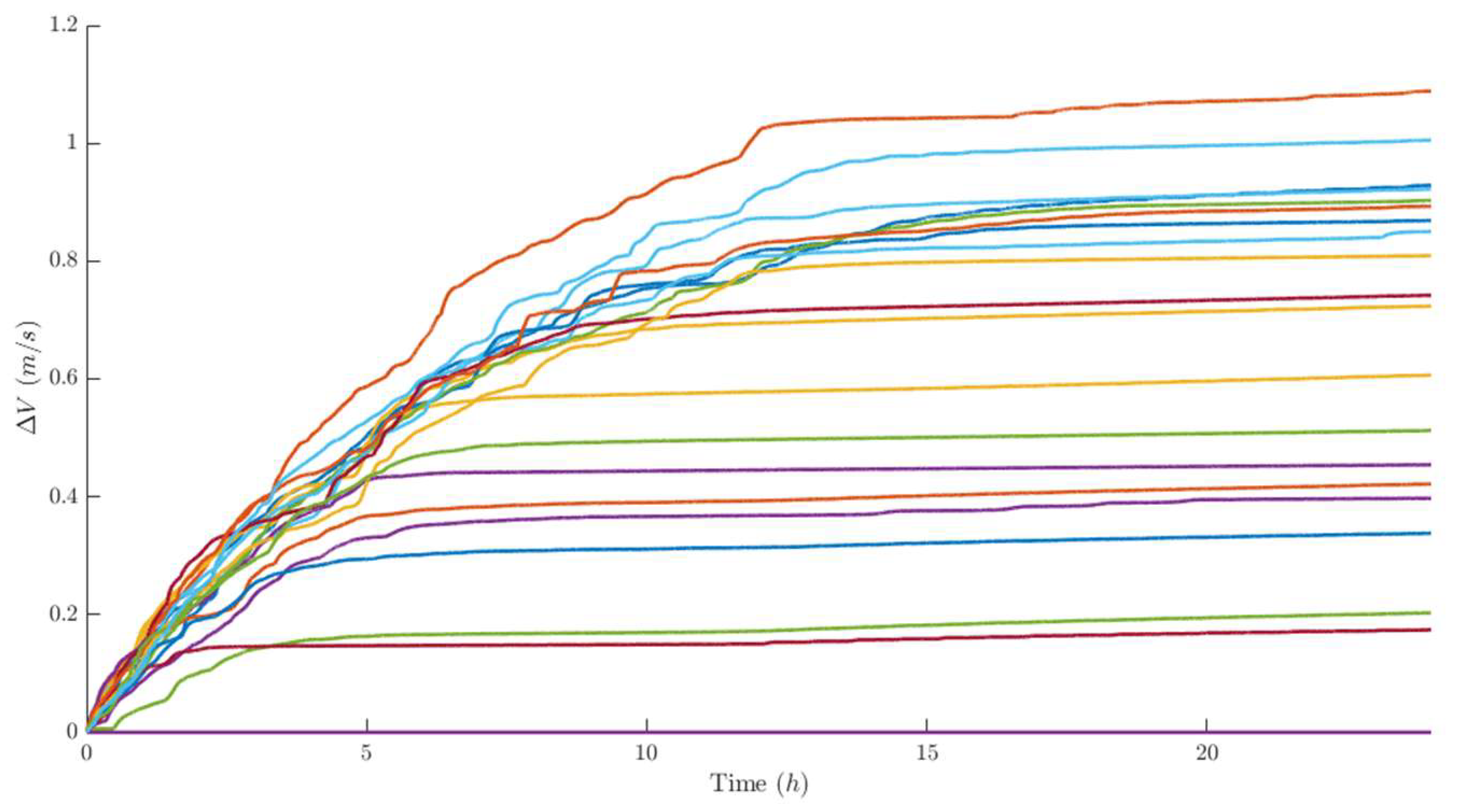
The control effort, summarized by the Δ
V reported in
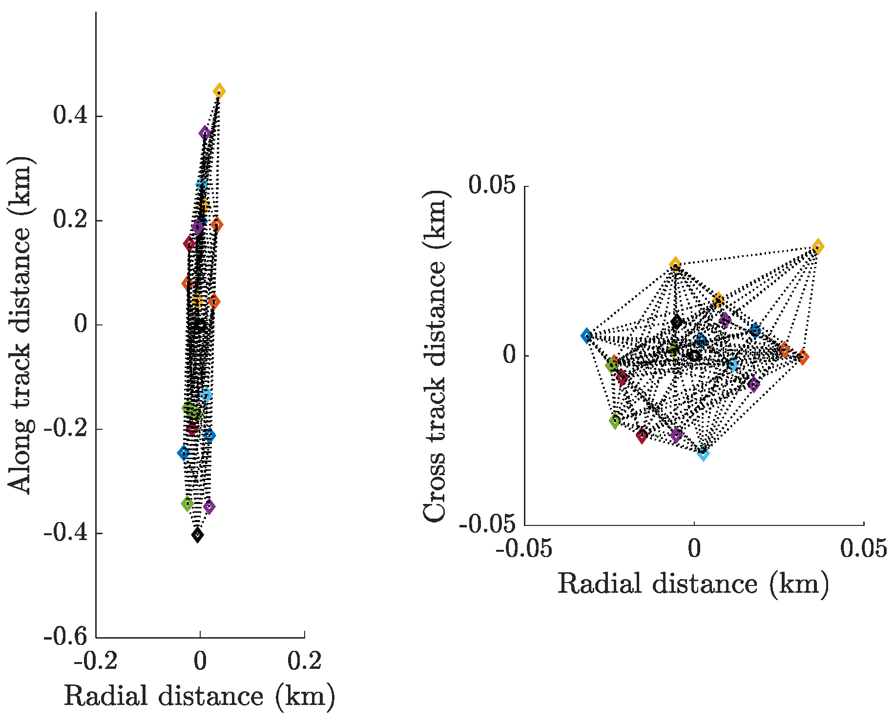
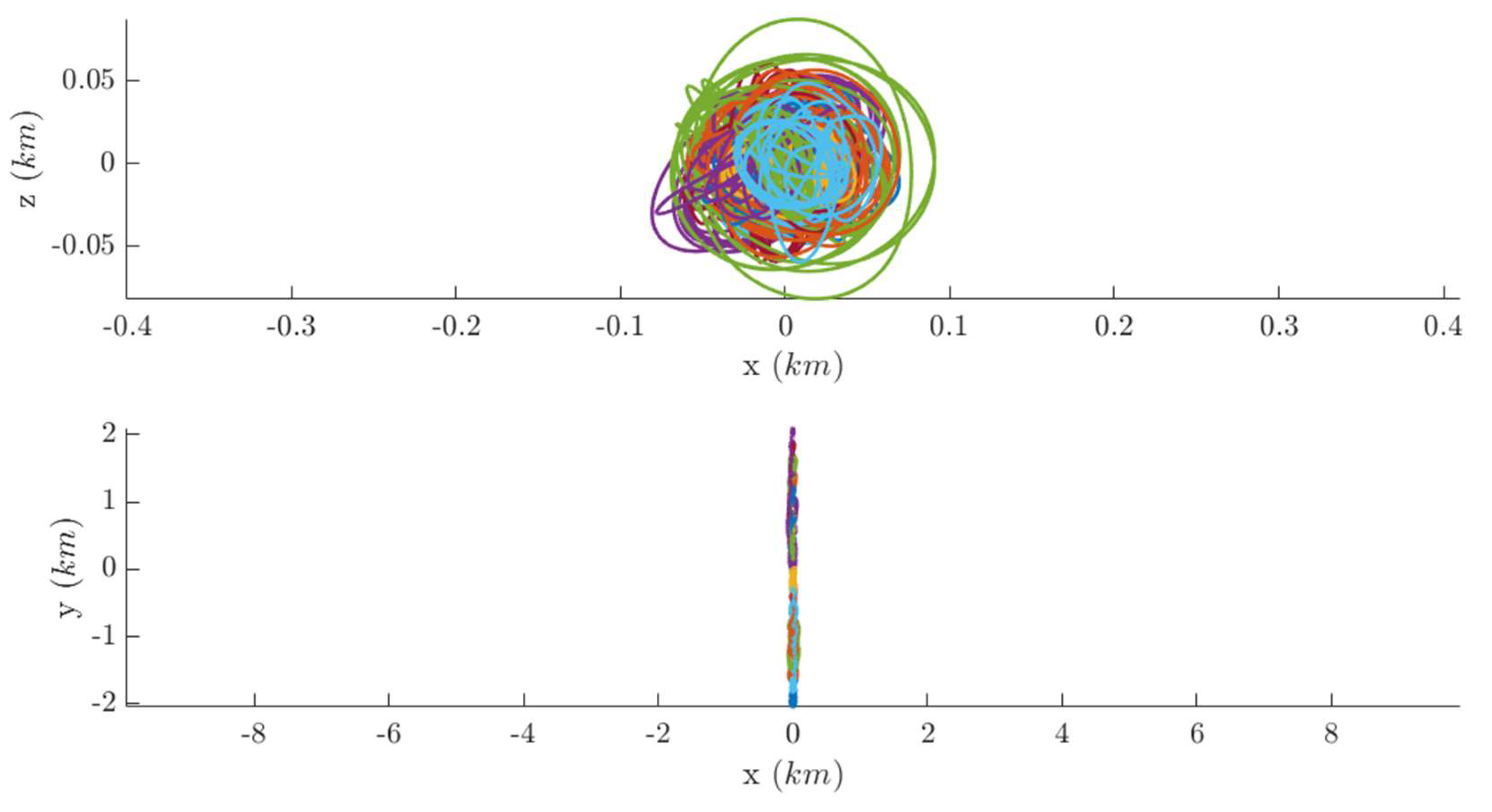
Figure 19 can be considered affordable and, more importantly, it reaches a stationary value, showing that the swarm behaviour is able to reach a stationary configuration where no more corrections are needed. In order to have a clearer view of the actual swarm dynamics, also the trajectories in the LVLH frame are reported in
Figure 20 (where the along-track behavior suggest a uniform distribution of the agents) and
Figure 21 (where it is possible to appreciate the XZ and XY projections of the trajectories).
5. A rough relative navigation system
One of the main objectives of this study is to assess whether behavioral control strategies can be effectively implemented using a highly simplified relative navigation system based on a single monocular camera and the comparison of successive image frames, without resorting to complex image processing, filtering, or target identification techniques. This approach is motivated by the need to minimize onboard computational requirements, which are particularly constrained on microsatellite platforms.
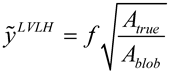
To this end, a blob-based image processing method [
22] is adopted to extract the apparent area (in pixels) of each visible satellite and the coordinates of its centroid in the image plane. These two quantities, evaluated over two consecutive image frames, provide sufficient information, in principle, to estimate the key relative parameters required by the behavioral control strategy. Of course, noise associated with real images must be considered, since they deeply affect the performance.
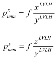
Assuming a pinhole model of the camera [
23], the coordinates in the image plane are proportional to the actual coordinates in the LVLH frame following the relation:
Where
,
are the blob coordinates in the image plane,
f is the focal length and
,
are the radial, along-track and cross-track distance, which is unknown but could be measured by a range sensor, or estimated with more sophisticated angles only navigation. In this paper, in the optics to keep the algorithm as simple as possible, the range is roughly computed considering the ratio between the area in the image plane and the real area.
The satellites are modeled as a central body (a square of 20 cm side) with two lateral solar panels (50 cm each). In
Figure 22, the B/W images of the satellites acquired and processed by another agent during a certain time lapse are represented as black blobs on a white background, as an example. When the satellites are not plotted, it means that at that time it is not in visibility (because it is too far or outside the FOV).
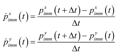
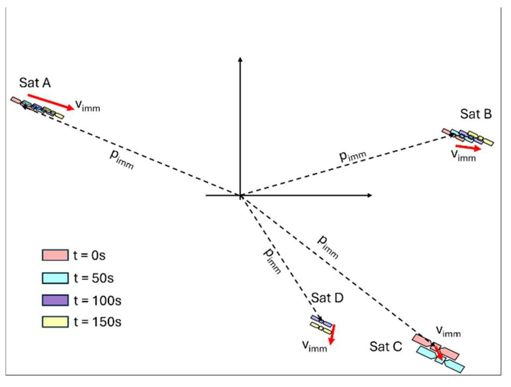
Considering two successive images, it is possible to easily associate the blobs to the same satellite by means of a nearest neighbor criterium. Therefore, a velocity in the image plane can be computed by finite difference of the recorded position in the image plane (see
Figure 23 for an explicative sketch).
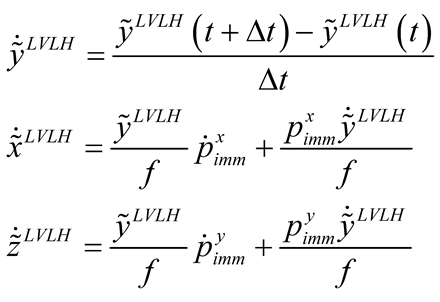
From these computations, the along-track, out-of-plane and cross-track velocities can be estimated:
The relative coordinates in the LVLH frame and the differential mean orbital elements are related by the following equations [
16]:
Running the same simulation of
Section 4.2 while taking this rough estimation of relative state
X into account, and analyzing the performance indices, it is possible to see that they are not greatly degraded: the integrity of the swarm is always achieved, the distance (
Figure 24) among the satellite in visibility confirms that no collision happens, and the minimum along-track distance of 100m is always respected. Concerning the transverse behavior,
Figure 25 and
Figure 26 are encouraging, being always greater than the minimum of 30 m, and the parallelism is respected in all cases, as shown in
Figure 27. The control cost, represented by the required
, is not qualitatively different: in fact, a total value of 12.84 m/s for the 20 members is required, while 11.42 m/s is requested in the ideal case of perfect knowledge. The real and important difference is that in the ideal case the control of the swarm reaches a stationary condition in which no further actions are needed (flat
behavior of
Figure 19), while using images there is a slight increase of the
required also in the last phases of the simulation (
Figure 28).
This satisfactory performance is due to the fact that here the ideal hypothesis that area and center of mass of the observed satellite is perfectly measured in the image plane is assumed; therefore, the only error is in the computation of the velocities as finite differences.
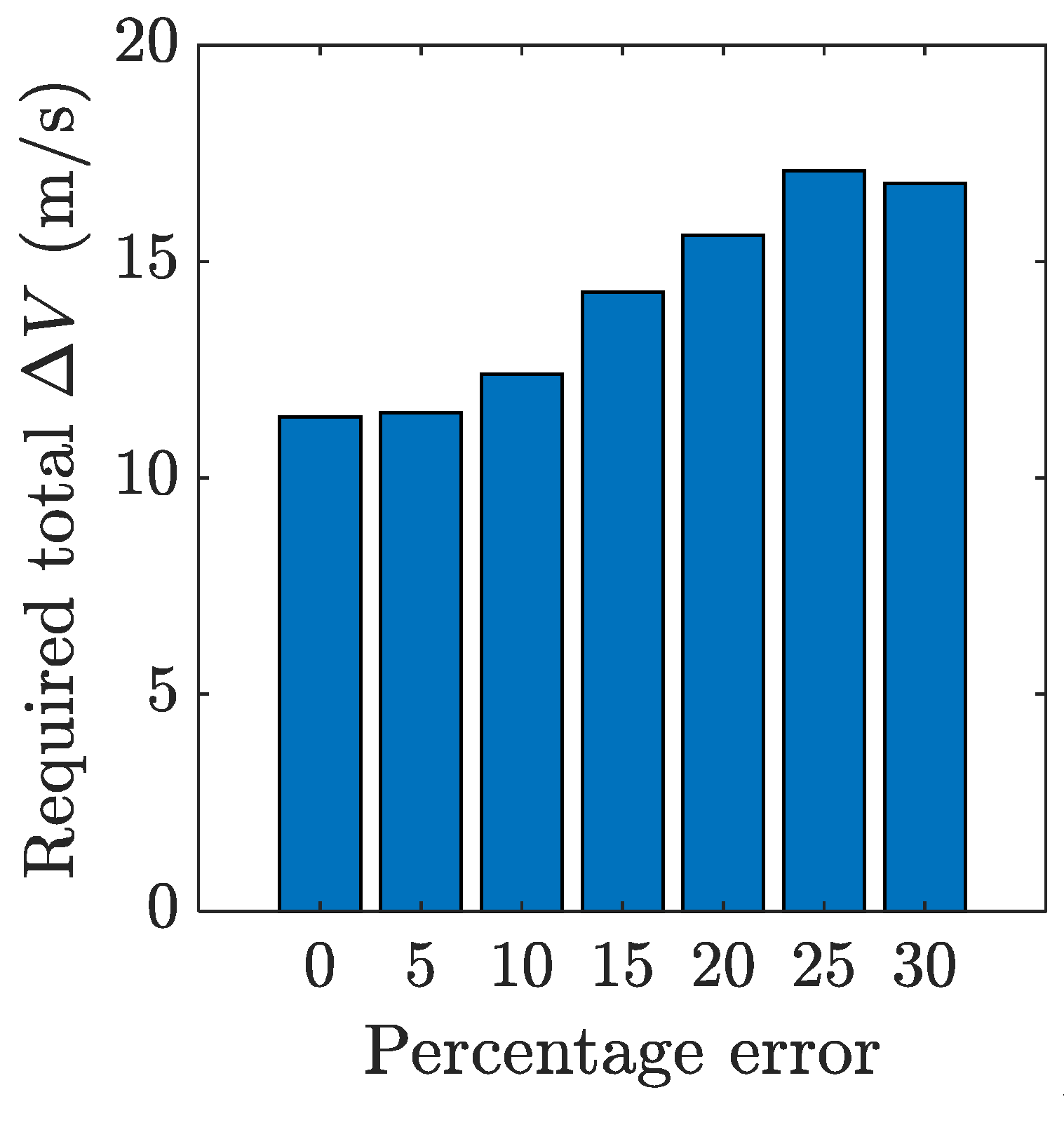
In order to give a qualitative information about the performance that a navigation system should have to implement the behavioral strategy, the simulation is now re-run by using differential orbital elements with additional gaussian noise equal to a certain percentage of its true value (from 0% (ideal) to 30 %).
Figure 29 shows how the global Δ
V required grows considerably with the navigation error. For a value of 30% noise level, the swarm loses its integrity, and therefore it must be considered an upper-bound (see
Figure 30).
6. Final remarks
This work has investigated the applicability of behavioral control strategies, originally developed in the field of robotics, to the autonomous maintenance of satellite swarms. The objective is to achieve a cohesive, drift-free formation with inherent collision safety, without relying on centralized supervision or coordination.
The results demonstrate that, under favorable initial conditions (specifically, when the swarm is initially connected), stable and safe configurations can be attained using simple, fully decentralized control actions computed onboard each spacecraft from a minimal sensor suite consisting essentially of a monocular camera.
At the same time, relative navigation remains a critical challenge. The analysis shows that inaccuracies in relative state estimation can degrade control performance and increase control effort. An upper bound on the admissible navigation error has therefore been identified, providing a quantitative requirement for the navigation algorithms (e.g., angles-only approaches) used to estimate the relative motion. Importantly, this bound is shown to be relatively permissive, indicating that behavioral strategies do not require highly sophisticated or computationally demanding navigation solutions.
Overall, the behavioral control framework presented in this study, although evaluated at a qualitative level, exhibits promising characteristics that motivate further investigation and development toward practical on-orbit implementation.
References
- Desai, J.P.; Ostrowski, J.P.; Kumar, V. Controlling formations of multiple mobile robots. In Proceedings of the 1998 IEEE International Conference on Robotics & Automation, Leuven, Belgium, May 1998.
- Gazi, V. Swarm aggregations using artificial potentials and sliding mode control. In Proceedings of the 42nd IEEE Conference on Decision and Control, Maui, HI, USA, December 2003. [CrossRef]
- Gazi, V.; Passino, K.M. Stability analysis of swarm. IEEE Trans. Autom. Control 2003, 48, 692–697. [CrossRef]
- Dorigo, M.; Trianni, V.; Sahin, E.; Groß, R.; Labella, T.H.; Baldassarre, G.; Nolfi, S.; Deneubourg, J.L.; Mondada, F.; Floreano, D.; Gambardella, L.M. Evolving self-organized behaviours for a swarm-bot. Auton. Robots 2004, 17, 223–245. [CrossRef]
- Ayre, M.; Izzo, D.; Pettazzi, L. Self-assembly in space using behaviour-based intelligent components. In Towards Autonomous Robotic Systems (TAROS), Imperial College, London, UK, September 2005.
- Izzo, D.; Pettazzi, L. Autonomous and distributed motion planning for satellite swarm. J. Guid. Control Dyn. 2007, 30, 449–459. [CrossRef]
- Clark, P.E.; Curtis, S.A.; Rilee, M.L. ANTS: Applying a new paradigm for lunar and planetary exploration. In Proceedings of the Solar System Remote Sensing Symposium, Pittsburgh, PA, USA, September 2002.
- Vane, D.; Stephens, G.L. The CloudSat mission and the A-Train: A revolutionary approach to observing Earth’s atmosphere. In Proceedings of the IEEE Aerospace Conference, Big Sky, MT, USA, 1–8 March 2008.
- Sabatini, M.; Reali, F.; Palmerini, G.B. Autonomous behavioral strategy and optimal centralized guidance for on-orbit self-assembly. In Proceedings of the IEEE Aerospace Conference, Big Sky, MT, USA, 7–14 March 2009.
- Sabatini, M.; Palmerini, G.B. Collective control of spacecraft swarms for space exploration. Celest. Mech. Dyn. Astron. 2009, 105, 229–244. [CrossRef]
- Reynolds, C.W. Flocks, herds, & schools: A distributed behavioural model. Comput. Graph. 1987, 21, 25–34. [CrossRef]
- Olfati-Saber, R. Flocking for multi-agent dynamic systems: Algorithms and theory. IEEE Trans. Autom. Control 2006, 51, 401–420. [CrossRef]
- Monakhova, U.; Ivanov, D.; Mashtakov, Y.; Shestakov, S.; Ovchinnikov, M. Communication area estimation for decentralized control of nanosatellites swarm. Acta Astronaut. 2023, 211, 49–59. [CrossRef]
- Kruger, J.; Hwang, S.S.; D’Amico, S. Starling Formation-Flying Optical Experiment: Initial operations and flight results. In Proceedings of the 38th Small Satellite Conference, Logan, UT, USA, 3–8 August 2024.
- D’Amico, S.; Ardaens, J.-S.; Gaias, G.; Benninghoff, H.; Schlepp, B.; Jørgensen, J.L. Noncooperative rendezvous using angles-only optical navigation: System design and flight results. J. Guid. Control Dyn. 2013, 36, 1576–1595. [CrossRef]
- Gaias, G.; Ardaens, J.-S. Flight demonstration of autonomous noncooperative rendezvous in low Earth orbit. J. Guid. Control Dyn. 2017, 41, 1337–1354. [CrossRef]
- Gaias, G.; Ardaens, J.-S.; Montenbruck, O. Model of J2 perturbed satellite relative motion with time-varying differential drag. Celest. Mech. Dyn. Astron. 2015, 123, 411–433. [CrossRef]
- Steindorf, L.M.; D’Amico, S.; Scharnagl, J.; Kempf, F.; Schilling, K. Constrained low-thrust satellite formation-flying using relative orbit elements. Adv. Astronaut. Sci. 2017, 160.
- Sabatini, M.; Palmerini, G.B.; Gasbarri, P. Control laws for defective swarming systems. In Proceedings of the Dynamics and Control of Space Systems (DyCoSS), Rome, Italy, 2014.
- Lewis, F.L.; Vrabie, D.L.; Syrmos, V.L. Optimal Control, 3rd ed.; John Wiley & Sons: Hoboken, NJ, USA, 2012; Chapter 3.
- D’Amico, S.; Montenbruck, O. Proximity operations of formation-flying spacecraft using an eccentricity/inclination vector separation. J. Guid. Control Dyn. 2006, 29. [CrossRef]
- Sabatini, M.; Volpe, R.; Palmerini, G.B. Centralized visual-based navigation and control of a swarm of satellites for on-orbit servicing. Acta Astronaut. 2020, 171, 323–334.
- Sturm, P. Pinhole camera model. In Computer Vision; Springer: Berlin/Heidelberg, Germany, 2014; pp. 610–613.
Figure 1.
Physical meaning of the relative orbital parameters. In-plane motion (left) and out-of-plane motion (right) illustrated in the Radial-Tangential-Normal (RTN) orbital frame (from [
18]).
Figure 1.
Physical meaning of the relative orbital parameters. In-plane motion (left) and out-of-plane motion (right) illustrated in the Radial-Tangential-Normal (RTN) orbital frame (from [
18]).
Figure 2.
Sketch of a j-th agent acquiring the position of only two satellites.
Figure 2.
Sketch of a j-th agent acquiring the position of only two satellites.
Figure 3.
Regions of repulsion (CA), alignment, and attraction.
Figure 3.
Regions of repulsion (CA), alignment, and attraction.
Figure 4.
Relative motion for parallel (top) and orthogonal (bottom)
δe/
δi vectors (from [
21]).
Figure 4.
Relative motion for parallel (top) and orthogonal (bottom)
δe/
δi vectors (from [
21]).
Figure 5.
Cross-track (above) and in-plane (below) behavior of two satellites performing a CA maneuver (blue: satellite 1, red: satellite 2): reference frame on COM of the swarm.
Figure 5.
Cross-track (above) and in-plane (below) behavior of two satellites performing a CA maneuver (blue: satellite 1, red: satellite 2): reference frame on COM of the swarm.
Figure 6.
XZ and XY coordinated plane projection of the relative motion under alignment action.
Figure 6.
XZ and XY coordinated plane projection of the relative motion under alignment action.
Figure 7.
Along-track separation of the uncontrolled swarm.
Figure 7.
Along-track separation of the uncontrolled swarm.
Figure 8.
Example of random initial configuration of the swarm.
Figure 8.
Example of random initial configuration of the swarm.
Figure 9.
Graph plot representing the swarm connectedness in the initial time.
Figure 9.
Graph plot representing the swarm connectedness in the initial time.
Figure 10.
Connectedness of the swarm.
Figure 10.
Connectedness of the swarm.
Figure 11.
Graph plot representing the swarm connectedness in the final time.
Figure 11.
Graph plot representing the swarm connectedness in the final time.
Figure 12.
First two differential mean elements of the ten satellites.
Figure 12.
First two differential mean elements of the ten satellites.
Figure 13.
Third and fourth differential mean elements of the ten satellites (differential eccentricity).
Figure 13.
Third and fourth differential mean elements of the ten satellites (differential eccentricity).
Figure 14.
Fifth and sixth differential mean elements of the ten satellites (differential inclination).
Figure 14.
Fifth and sixth differential mean elements of the ten satellites (differential inclination).
Figure 15.
Along-track distance of all satellites with respect to all respective closest visible satellites.
Figure 15.
Along-track distance of all satellites with respect to all respective closest visible satellites.
Figure 16.
Out-of-plane distance of all satellites with respect to all respective closest visible satellites.
Figure 16.
Out-of-plane distance of all satellites with respect to all respective closest visible satellites.
Figure 17.
Minimal radial distance of all satellites with respect to all respective closest visible satellites.
Figure 17.
Minimal radial distance of all satellites with respect to all respective closest visible satellites.
Figure 18.
Parallelism of all satellites with respect to all respective visible satellites.
Figure 18.
Parallelism of all satellites with respect to all respective visible satellites.
Figure 19.
Control performance in terms of ΔV required by each swarm member.
Figure 19.
Control performance in terms of ΔV required by each swarm member.
Figure 20.
Along-track position of the spacecraft with respect to the swarm center of mass.
Figure 20.
Along-track position of the spacecraft with respect to the swarm center of mass.
Figure 21.
Cross-track (upper subplot) and in-orbit (lower subplot) projections of the relative trajectories with respect to the swarm center of mass.
Figure 21.
Cross-track (upper subplot) and in-orbit (lower subplot) projections of the relative trajectories with respect to the swarm center of mass.
Figure 22.
Example of sequence of images recorded by a satellite of the swarm, observing two satellites on different trajectories.
Figure 22.
Example of sequence of images recorded by a satellite of the swarm, observing two satellites on different trajectories.
Figure 23.
Sketch of a scenario in which a certain agent is able to observe four satellites, some of them for all the time (Sat A, Sat B) and some others exiting the FOV (Sat C, Sat D).
Figure 23.
Sketch of a scenario in which a certain agent is able to observe four satellites, some of them for all the time (Sat A, Sat B) and some others exiting the FOV (Sat C, Sat D).
Figure 24.
Along-track distance of all satellites with respect to all respective visible satellites (rough navigation case).
Figure 24.
Along-track distance of all satellites with respect to all respective visible satellites (rough navigation case).
Figure 25.
Minimum radial distance of all satellites with respect to all respective visible satellites (rough navigation case).
Figure 25.
Minimum radial distance of all satellites with respect to all respective visible satellites (rough navigation case).
Figure 26.
Out-of-plane distance of all satellites with respect to all respective visible satellites (rough navigation case).
Figure 26.
Out-of-plane distance of all satellites with respect to all respective visible satellites (rough navigation case).
Figure 27.
Parallelism of all satellites with respect to all respective visible satellites (rough navigation case).
Figure 27.
Parallelism of all satellites with respect to all respective visible satellites (rough navigation case).
Figure 28.
Control performance in terms of ΔV required by each swarm member (using images).
Figure 28.
Control performance in terms of ΔV required by each swarm member (using images).
Figure 29.
Control performance in terms of total ΔV required for different errors affecting the navigation system.
Figure 29.
Control performance in terms of total ΔV required for different errors affecting the navigation system.
Figure 30.
Connectedness of the swarm for a noisy measurement (35% standard deviation).
Figure 30.
Connectedness of the swarm for a noisy measurement (35% standard deviation).
Table 1.
Alignment algorithm.
Table 2.
Initial conditions in terms of relative orbital elements.
Table 2.
Initial conditions in terms of relative orbital elements.
| Differential o.e. |
Expression |
Standard deviation σ (m) |
| Semimajor axis, a
|
σa |
50 |
| Eccentricity, e
|
σe/a |
50 |
| Inclination, i
|
σi/a |
50 |
| Argument of perigee, w |
σw/a |
50 |
| RAAN, Ω |
σΩ/a
|
50 |
| True anomaly |
σan/a |
1000 |
|
Disclaimer/Publisher’s Note: The statements, opinions and data contained in all publications are solely those of the individual author(s) and contributor(s) and not of MDPI and/or the editor(s). MDPI and/or the editor(s) disclaim responsibility for any injury to people or property resulting from any ideas, methods, instructions or products referred to in the content. |
© 2026 by the authors. Licensee MDPI, Basel, Switzerland. This article is an open access article distributed under the terms and conditions of the Creative Commons Attribution (CC BY) license (http://creativecommons.org/licenses/by/4.0/).

 (7)
(7)

 or
or 
 or
or