
Submitted:
15 January 2026
Posted:
19 January 2026
You are already at the latest version
Abstract
Previous studies have found that interaural cross-correlation (IACC) and lateral energy fraction (LF) can serve as objective measures to predict apparent source width (ASW). However, there is a lack of literature regarding how well objective measurements correlate with subjective evaluation in a context-dependent scenario. Expanded upon a prior work, this study looked to examine the extent to which commonly assumed predictors of ASW remain valid when applied to real concert hall measurements across listener positions. ASW ratings were obtained through psychoacoustic tests employing both stereo loudspeakers and headphones to assess the perceived width of a symphony orchestra produced with different recording techniques and ensemble sizes. Key room acoustic parameters were calculated from impulse response measurements conducted in the EMPAC concert hall in Troy, NY, where the orchestral recordings were made. Results show that the existence and emergence of ASW is based on the opposite perceptual mappings between the two reproduction conditions, even though stereo loudspeakers resembled real hall listening more closely. The findings also suggest that assuming a fixed role of binaural decorrelation for enhancing ASW is impractical because ASW is governed by context-dependent object integration, where binaural decorrelation is only beneficial when it supports rather than disrupts object unity.
Keywords:
apparent source width
; auditory spatial impression
; room acoustics
; binaural hearing
; aural architecture
; sound field reproduction
1. Introduction
30 years ago, Leo Beranek and his colleagues published a series of crucial works in linking listening experience in concert halls with quantifiable measures and in underpinning what comprises a quality spatial perception of musical performances [1,2]. Auditory spatial impression (ASI), an official term to characterize how listeners perceive the acoustical quality of performance spaces, is formed by identifying spatial attributes among other psychoacoustic attributes (such as clarity and warmth) as the determining factor of the impression of an aural architecture. Among the spatial attributes that contribute to auditory spatial impression, as argued by Beranek et al., apparent source width (ASW) and listener envelopment (LEV) are of major interest. Since then, abundant writings and professional applications followed the trend of evaluating lateral reflections, binaural correlation and decorrelation, and ensemble width in aiding both architectural design and sound design [3,4,5,6,7,8,9,10,11,12,13,14].
After Wallace Clement Sabine concluded his law of reverberation [15], researchers realized that not only the time for the precise auditory localization of the sound source to remain unaffected if the direct and the reflected sound could arrive completely to the ears is short, but also the perception of the direct sound could be enhanced, whether with increased loudness, richness, or clarity, if the reflected sound within that short time range is boosted [16,17,18,19]. Consequently, as an outcome of more interest put on the early signal structure rather than the entire decay tendency a room presents, defining room acoustical descriptors other than reverberation time (RT) have emerged, which now become the internationally standard parameters [20].
These parameters characterize the room by the perceived clarity, the early sound decay behavior, the average arrival time of the sound energy, the lateral strength of the sound energy, and the degree of binaural similarity. Although the concept of reverberation time assumes a diffuse sound field in which other parameters that emphasize the early short time window do not, there are prominent similarities in why reverberation time and the other ones always appear together in modern room acoustical practices. First, all the parameters mentioned, including reverberation time, are now calculated from an impulse response of the room in which a linear time-invariant system (LTI) becomes the common assumption. Second, both RT and the early-field descriptors reduce the wave field to an energy-time representation, where the former presents the probabilistic energy mixing and the latter portrays the deterministic energy transport. Third, both sets of parameters express the macroscopic acoustic behavior above the Schroeder frequency [21] without solving the wave equations that describe the instantaneous pressure variations, the phase-coherent interference, the diffraction, the boundary conditions, and the standing wave patterns.
As a dominating factor for auditory spatial impression, apparent source width is believed to be tied closely to two of the aforementioned objective acoustical measures—interaural cross-correlation coefficient (IACC) and lateral energy fraction (LF). The explanation is that, in the early short time window (0 to 80 milliseconds), where major auditory processing, such as localization, intelligibility, and source widening, is formed, reflections from the sides cause binaural time and level differences that result in the fluctuations of the binaural similarity, affecting the final perception of the source image. Thus, the belief is that the more side reflections represented by the spatial structure, the more the binaural effect of signal decorrelation (lower IACC), which controls the increased apparent source width as a final perceptual outcome. Profoundly, as a description of how the room delivers energy to the listener in time, direction, and spectrum, room acoustic parameters reveal the direct consequences the physical room structure produced on the binaural cues in which apparent source width sits on top. The perceptual width of a musical entity is the result of binaural encoding through the integration of the energy structure constructed in the auditory system. There is a broader connection to the relationships between apparent source width and these physical and binaural acoustic mechanisms that is yet to be discovered.
In a previous study, the author mentioned how important the perception of an apparent wideness of the performing entity is to what is commonly considered “listening sensitive” scenarios [22]. Though seldom stated explicitly, the desire for a counterintuitive comprehension in which a perceived “enlargement” is able to be delivered to the sensory, nervous, and cognitive system through a mismatch between the auditory and the visual input in a positive way is the core that generates satisfaction in a composition, a record, or a performance space. For architects, this percept directly influences how listeners judge the quality of a concert hall. Griesinger in 1997 has pointed out that the quantification processes done by different scholars for spatial impression, particularly for apparent source width, have been inconsistent [23]. In fact, this inconsistency continued over the decades.
After the established view proposed by Leo Beranek et al., Matthias Blau examined three objective measures for apparent source width. He found that in situations where single reflections dominate, (a binaural impulse response with respect to the angle of incidence predominately in the frontal plane) may describe apparent source width more precisely, although the potential may occur when outperforms the other measures when a criterion is set upfront for dividing the sound fields according to its level of diffusiveness [24]. In the context of reproducing a sound field with reliable attributes of auditory spatial impression, Hyunkook Lee studied the importance of distance between source and receiver with respect to both apparent source width and listener envelopment. Lee’s results agreed with Barron and Marshall’s and with Leo Beranek’s findings on how sound pressure level (SPL), or sound strength (G), affects spatial impression (including both ASW and LEV), but less agreed with the findings on whether interaural cross-correlation (IACC or 1-IACC) or lateral energy fraction (LF) are major factors on affecting apparent source width and listener envelopment [25]. However, in studying the effects of two-channel stereo reproduction on apparent source width, Johannes Kasbach et al. proved that the inter-channel correlation (IC), or the interaural crosstalk, has an inverse relationship to apparent source width, and interaural cross-correlation (IACC) can agree with ASW data when inter-channel correlation (IC) is low, although the opposite is not true [26]. This finding was partially in line with the widely held view that a high degree of apparent source width demands a low correlation between the ears. Consequently, the idea of increasing apparent source width by decreasing the interaural correlation has been applied by Guillaume Potard and Ian Burnettin [27] and by Carlotta Anemuller et al. [13] in designing sound effects to improve the perceived naturalness of the sound sources. Another finding that aligned with scholars mainly investigating concert hall acoustics was obtained by Arthi S. and T. V. Sreenivas, that low frequency signals help broaden the width of a perceived sound source, and a continuing signal may elicit a wider width of the source compared to a transient signal [12]. Furthermore, Olli Santala and Ville Pulkki provided some insight into auditory perception of spatially distributed sources based on different source distribution arrangements and different signal bandwidths [28]. Santala and Pulkki confirmed that a certain amount of evenly distributed sound sources helps the auditory system to form a whole in the perception of source width, and the narrower the signal bandwidth is, the harder it is for the auditory system to discriminate its location.
Nevertheless, apparent source width should not inherently be considered as a single modal percept. Indeed, the studies conducted by Daniel Valente and Jonas Braasch over the years have attested to the strong inverse relationship between vision and auditory perception that the more visual cues involved in the judgment of an auditory event in the context of spatial impression, the less correct the auditory judgment will be for a given enclosed space with a given number of performers [29,30,31]. As stated earlier, while this audio-visual mismatch may be interpreted as a negative, it could more likely be regarded as an evaluating point for the magic played by a pleasantly wide perceived source width. Whether implicitly as an integrated sensory product from multiple modalities or as a definition baffled by methodological inconsistency, the percept of apparent source width certainly requires deeper understanding and more comprehensive evidence.
Built upon a previous study investigating how stereo recording and reproduction and physical source width impact the spatial perception of the sound source, this paper aims to take a further look into how ASW emerges from acoustical and binaural structure and to evaluate the extent to which commonly assumed predictors of ASW remain valid when applied to real concert hall measurements across listener positions. Thus, this study brings a coherent comparative framework with a dataset that contains room acoustic measurements and psychoacoustic experiments, and looks to contribute in a layered way in which the links across physical, binaural, and perceptual levels are explicitly examined.
2. Method
A psychoacoustic experimental dataset, collected from the author’s previous study [22], was used in the current research. Room impulse response measurements were conducted across 16 different seating locations at EMPAC concert hall. 4 seats were selected for data analysis in this paper to correspond to the orchestral recording positions in the front and middle rows. At each seat, a 4-channel impulse response was captured under consistent measurement conditions.
2.1. Psychoacoustic Experiment
2.1.1. Test Stimuli
A total of 30 recording clips were produced by rendering an anechoic orchestral record through wave field synthesis (WFS) linear array in EMPAC concert hall, and capturing it using five microphone techniques: spaced omni, ORTF, mid-side (MS), Blumlein, and binaural. The virtual orchestra was presented in three ensemble settings—orchestral, stereo, and mono—to represent different physical source widths on stage. All recordings were made at two distances away from the stage: front row and mid row. The recording clips were excerpts (25 seconds each) from the first movement of Beethoven’s Symphony No. 8, bars 45 to 72.
2.1.2. Playback
Two playback methods were used: stereo loudspeakers and headphones. For stereo loudspeakers, playback took place in a small, professionally treated room (dimensions: 3.76 m × 3.0 m × 2.45 m) equipped with JBL 308P MKII monitors arranged in an equilateral triangle configuration relative to the listener. Loudspeakers were connected to a FocusRite 4i4 audio interface. No crosstalk cancellation was applied to binaural recordings. For headphones, playback was conducted using a Beyerdynamic DT 770 Pro headphone in the same listening environment.
2.1.3. Participants
A total of 11 male participants with normal hearing took part in the study: 7 subjects for the loudspeaker experiment and 4 subjects for the headphone experiment. All participants were undergraduate students enrolled in audio and acoustics courses at Rensselaer Polytechnic Institute, aged between 19 and 21.
2.1.4. Test and procedure
Listeners were asked to rate the perceived width of the orchestra for each recording clip using a 7-point Likert scale, where 1 indicated a very narrow source width, and 7 indicated an extremely wide source width. Stimuli were presented in a graphical user interface (see Figure 1) with randomized order on a program in Python which allowed subjects to listen and submit responses interactively. No visual cues or scores were provided, and participants were not informed of the recording technique or ensemble configuration.
2.2. Impulse Response Measurements
2.2.1. Sending
The room excitation system included 3 loudspeakers placed on stage to cover the full audible frequency range. These consisted of a high-band omnidirectional loudspeaker, a mid-band omnidirectional loudspeaker, and a subwoofer for low-band content. Each loudspeaker was used to radiate a logarithmic sine-sweep signal into the room in sequence, making sure that the measured response reflected the room’s behavior across the entire spectrum.
2.2.2. Receiving
At each of the 16 receiver positions, a 4-channel measurement setup was used. This setup consisted of one omnidirectional microphone, one figure-8 microphone, and one binaural dummy head. Together, these three devices allowed for the collection of mono and binaural impulse responses from each seating location. The omni channel was used to derive conventional room acoustic metrics, such as reverberation time (T10, T20, and T30), early decay time (EDT), clarity (C50 and C80), definition (D50), center time (Ts), while the binaural channels and figure-8 were used to calculate spatial parameters such as lateral fraction (LF) and interaural cross-correlation (IACC).
2.2.3. Center Control
All measurements were performed using the EASERA software (Electronic and Acoustic System Evaluation and Response Analysis). The excitation signal was first generated in the computer and sent through an audio interface, which connects both the signal senders and the receivers. From there, the signal was routed to a speaker amplifier, which then drove the three loudspeakers (high-band, mid-band, and subwoofer) used as sound sources. The microphones picked up the room response and transmitted it through the audio interface to convert the signal into digital form. The signal processing chain is showed in Figure 2. Each measurement duration is 5 seconds at 48k Hz sampling rate, consistent across all measurement positions.
2.3. Room Acoustic Parameters
Following ISO-3382-1 [20], 14 standard room acoustical parameters were calculated in MATLAB from the room impulse responses measured in EASERA, described below.
2.3.1. Peak-to-Noise Ratio
Unlike Signal-to-Noise Ratio (SNR), which compares the power of the signal to the power of the noise, Peak-to-Noise Ratio (PNR) compares the peak amplitude of the signal to the root mean square amplitude of the noise, and takes rather than consequently (see Equation (1)). Thus, while SNR provides a general description of the validity of the room acoustic measurement, PNR provides more insights into how valid a transient signal maintains its integrity under a particular measurement system.
Where is the peak amplitude of the measured impulse response , and is the average noise power, which is defined as:
2.3.2. Clarity Indices
Also known as sound energy ratios, the clarity indices (C50 and C80) compare two parts of sound energy based on two time windows (see Equations 2 and 3). For example, the time windows for C50 are 0 ms to 50 ms (early time window) versus 50 ms to the last millisecond of the impulse response (late time window). The result of the ratio tells which part of the sound energy in the impulse response dominates and is expressed in decibels. C50 is used typically for speech signals, and C80 is used for orchestral music signals.
2.3.3. Definition
Definition (D50) is also a type of energy ratio that compares the sound energy in the early time window versus the sound energy in the entire time window of the impulse response. Different from clarity indices, definition is used exclusively for speech signals and is expressed as a percentage (see Equation (4)).
2.3.4. Center Time
Analogous to the center of gravity in mechanics, where the average position of a mechanical system is weighted by its mass distribution, center time (Ts) reveals the average arrival time of sound energy of an acoustical system, namely, a room. In a room impulse response measurement, stronger sound energy pulls the average temporal position toward it, resulting in a shorter or longer arrival time that indicates a clearer or more reverberant room acoustic. The center time can be measured in seconds or milliseconds (see Equation (5)).
2.3.5. Reverberation Time
After Schroeder proposed the groundbreaking new method to measure reverberation time in 1965 [32], the calculations for reverberation time (T10, T20, T30 approximation) and early decay time (EDT) use directly the sound energy integrated backwards of an impulse response to correspond to how much sound energy are left in the room as a function of time if the sound source stopped vibrating. This integration is then normalized to 0 dB to show the sound energy decay (switch-off decay in the historical context) on which the reverberation time is based (see Equation (6)). The slopes (decay rates) from different ranges of the energy decay curve (EDC) are extrapolated to approximate the reverberation time T60 in different temporal perspectives for analytical precision and comparisons (see Table 1).
2.3.6. Lateral Energy Fraction
As another type of energy ratio, lateral fraction (LF) compares the early sound energy that comes from lateral directions, such as from the sides, to the energy that comes from all directions. Correspondingly, one omni microphone and one figure-8 microphone should be applied in the measurement for the LF calculation, and the direct sound that comes from the front should be excluded from the lateral energy time window for data clarity. (see Equation (7)) It is believed that the value of LF correlates directly with auditory spaciousness. The higher the value, the greater the early lateral energy, the wider image the sound source, and thus the more sense of spaciousness. Lateral fraction is unitless with values ranging from 0 to 1 (or to ).
2.3.7. Lateral Energy Fraction Calibrated
A calibrated version of lateral fraction was brought up because Mendel Kleiner [33] believed that in order to keep the original resolution of the figure-8 radiation pattern, the numerator of the LF equation (see Equation (7)) should not be the squared impulse response received in the figure-8 pattern which is equivalent to because of the distortion of the radiation pattern (see Figure 3). Instead, Kleiner proposed to multiply the two amplitude responses from the omni and figure-8 channels as a cross-term to better address how much the lateral signal has projected onto the omni field (see Equation (8)). The sound source, regardless of its size, radiates acoustical energy from the stage to the audience area with countless reflections from the sides, whether specular or diffuse, directed toward the audience. While LF informs how strong the early reflections from the sides are, LFC may tell more about how well-directed those early side reflections are toward the target audience.
2.3.8. Interaural Cross-Correlation
In room acoustics, interaural cross-correlation measures the degree of similarity a signal is perceived by our left and right ears, described in Equation (9). While the general cross-correlation function in signal processing reveals the relationship between two signals in a diagnostic manner, telling information about the delay time, the similarity strength, the secondary peaks, and the polarities of one another, the interaural cross-correlation function focuses on how much the left and right ear signals resemble each other within the range that the human head allows (usually between -1 and +1 millisecond as the maximum range of interaural time difference). Furthermore, instead of having its value fall between -1 and +1 as a typically normalized result of a correlation function which is widely applied in DSP, the more interested part for interaural cross-correlation coefficient is the maximum absolute magnitude that falls between 0 and 1 to correspond to the nature of human hearing in which time and level difference is more sensitive than polarity and phase difference.
3. Results
3.1. Calculated Room Acoustic Parameters
Table 2 shows all the parameter values for each seat calculated in broadband. The table as a whole denotes a sound field with fairly well-distributed sound energy diffused from the room reflections that tend to be ideal. The Peak-to-Noise Ratio goes down with the increase in distance, which is common sense, but not to a point where the sound energy is dissipated at the end of the distance because the hall reflections enhanced it. The C80 values represent a typical concert hall where the musical details (instrument locations, timbre differences, notes) are preserved at farther seats, although the direct sound and the early reflections lose dominance at these positions. Similarly, the C50s and D50s indicate that listeners are certainly able to distinguish a speech signal coming from the stage with more or less unintelligibility depending on the spectrum of the voice, because the hall is not initially designed for speech after all. The temporal parameters (Ts, EDT, T10, T20, T30) tended to increase with the increase of distance, yet this tendency stopped at seat 3, and then it dropped back as distance continued to go forward.
Meanwhile, it seems clear that the differences between the reverberation times across the receiving positions are not much, and the data follows a progression tendency in which EDT < T10 < T20 < T30, signifying a balanced room with smooth transition from early to late energy decay. According to the lateral energy fraction equations (see Equations (7) and (8)), it is highly expected that every LFC value is lower than or equal to its corresponding LF value, which is the case in this measurement data, because will hardly exceed unless is significantly larger than . These LF and LFC data showed a fair amount of early lateral energy, which is a sign of a strong sense of spaciousness, but only starting from a certain distance (seat 3) and beyond.
However, the IACC values complemented the LF data by which the low early lateral fractions presented in the front seats are an indication of a somewhat focused but not narrowly localized sound field, rather than a dead or dry field with poor sense of spaciousness. Furthermore, as spatial parameters, both LF and IACC showed no sign of a shrinking sound image with the increase of distance, which is often considered plausible. Overall, while the temporal parameters (specifically reverberation time and early decay time here) may indicate an ideal diffuse field due to their high similarities, the energy ratios and spatial parameters reveal a gradually changing sound field with distinct auditory spatial image for each seat that is hardly to be “equal”.
3.2. Correlation Between and C80, EDT, T30, and LF
Scatter plots and correlation coefficients r are applied to understand the relationship within parameters, specifically, between interaural cross-correlation () and early decay time (EDT), reverberation time (T30), lateral energy fraction (LF), and clarity (C80), showed in Figure 4. The result of a correlation is displayed separately with different color-coding to see a paired visualization with spatial and spectral emphasis. Taking the vs. EDT as an example, one plot is showing the correlation with seat information being explicit, and the other one is showing the same correlation with explicit frequency information. The number of data points on these two plots are exactly the same, which is 21 3rd octave band center frequencies times 4 seats equals 84 data points, because essentially, they are one plot in different presentation forms that has the same data pattern as well.
From an overall look, the temporal correlations ( vs. EDT and vs. T30) presented ascending trends with r values being positive, and the energy ratio correlations ( vs. C80 and vs. LF) presented descending trends with r values being negative. For the temporal correlations, T30 showed stronger positive relationship to than EDT did. Note that one should not mix up these correlation results with the broadband parameter results (showed in Table 2) because they are due to different mechanisms even though they appear plausibly contradictory. For example, the scatter plots for and T30 here represent the within-seat frequency-dependent relationship, showing that higher T30 leads to higher per seat across frequency, while Table 2 represents the between-seat comparison, showing that longer T30 tends to have lower across different seats. The reason for EDT to be correlated less with than T30 does is that even though uses only the early portion of the impulse response, it is still influenced by the shape of the entire room’s early–mid decay structure, which often aligns more with the slope seen in T30 than with the very first 10 dB of decay. In other words, within the 80 millisecond window, factors such as the energy build-up, the diffusion quality, and the lateral reflection density are capable enough to influence , and these factors symbolize the early-to-late transition of the decay curve, which is the region covered by T30 instead of EDT. Because T30 tracks more of the room’s reflected energy, features signifying spatial hearing, such as the early lateral reflection density, the perceived envelopment, and the binaural correlation, are in turn influenced more. Hence, the correlation between T30 and tightens. Meanwhile, the scatters also reveal that EDT varies dramatically with seat location under the influence of direct sound arrival angle and local early reflections while T30 presents more global reverberant field characteristics, suggesting a more seat-dependent fact for EDT versus a more room-dependent T30.
Furthermore, the complementary frequency content scatters show that not only EDT exhibits substantially greater variability across seat positions compared to T30, but it also varies much more with frequency than T30 does. For both T30 and EDT, as both time and increase, frequencies become lower. For example, frequencies lower than 400 Hz have above 0.8 and T30 above 2.5 seconds, while frequencies higher than 4000 Hz mostly have below 0.6 and T30 below 2 seconds. Overall, the T30 result scatters less widely horizontally than the EDT one, and the low-mid range (below 400 Hz) forms a stronger monotonic trend with a less chaotic high range (above 2000 Hz).
For the energy ratio correlations, the negative r values in both C80 and LF plots indicate the part of the sound field that reduces , in which the greater early energy and the more lateral fraction lead to less binaural coherence. Strong early and lateral reflections presented in C80 and LF create large interaural time and level differences which are crucial for decorrelating a signal between the ears. Meanwhile, C80 correlates with more strongly than LF does, especially at further seats. The reason is that, compared to what C80 captures, LF has a more specific and constrained energy portion to concern about. This means that LF aligns less with due to its exclusion of the direct sound, the frontal, ceiling, and backward reflections, leading to a limited geometrical variability and a tighter spectrum cluster. For example, front seats showed nearly flat slopes and little frequency movements in the 3rd octave bands in LF. On the other hand, C80 aligns much better with with more fluctuations across frequencies and space and stronger slopes for further seats, implying the dominance of is the buildup of early reflections where directionally uneven, band-wise diverse early-to-late balance affects binaural differences strongly with even a small change.
In the frequency-coded complementary plots, both C80 and LF presented a difference between the high and the low frequency regions when correlate with . For C80, tight clusters occurred around positive values in the high bands (1600 Hz to 8000 Hz) where is moderately low (0.2 to 0.6), implying a stable downward trend where increasing the early energy decreases the binaural coherence. For LF, the majority of the high bands fell between 0.1 to 0.5, where these points nearly formed a strong negative line, showing specifically how lateral reflections decorrelate the ears at high frequencies. In the mid and low regions (below 1000 Hz), C80 spanned from -15 dB to +5 dB, and LF also ranged widely from 0.1 to 1, both with an increased threshold from 0.2 to 1 and a much more scattered pattern indicating a more diffused relationship. This means that because the head cannot create strong binaural asymmetry, both C80 and LF lose predictive power of at low frequencies.
3.3. Correlation Between ASW and and LF
The ASW correlation analysis, showed in Table 3, was performed by first computing mean ASW ratings across subjects for each recording clip and subsequently aggregating these values according to listener distance, corresponding to front and middle seating regions in the concert hall. The resulting aggregated ASW values were then associated with the receiver positions for which broadband parameters had been calculated, such that each measured seat was assigned a single ASW value. Pearson correlation coefficients were then computed across receiver positions between normalized ASW values and the corresponding and LF values. Unlike the within-parameter correlations in section 3.2, which were evaluated on a per-seat and per-frequency basis, the ASW correlations were conducted across-seat that resulted in a single correlation coefficient for each reproduction condition. In this context, the correlation coefficient reflects whether across the set of seats, ASW discriminate seating positions in the same direction as the objective spatial descriptors. For both loudspeaker and headphone reproduction conditions, the correlation presented strong linear relationships between mean ASW ratings and their corresponding objective measures.
While the strong magnitude of the correlations remained identical between the two reproduction conditions, the signs of the correlations differed consistently between conditions, such that ASW showed a negative correlation with and a positive correlation with LF under loudspeaker playback, whereas the opposite sign pattern was observed under headphone playback. In addition, the correlation between ASW and LF reached statistical significance in both reproduction conditions, whereas the correlation between ASW and did not meet the same significance criterion. In the ASW vs. correlation, the loudspeaker playback presented what classic literature have been believed: lower leads to wider apparent source whereas higher leads to narrower source perception, and thus listeners’ ASW judgements follow the binaural decorrelation of the signal a room displays. However, this belief is no longer valid for headphone playback conditions, as listeners may not believe a higher is equivalent to a narrower source, but rather to an impression that is “stable” or “spatially coherent”. Subsequently, when ASW correlate with LF, the mirrored story occurred again. The loudspeaker condition conforms to the fundamental assumption that strong lateral reflections lead to strong binaural decorrelation, which causes broader spatial impression. For headphones, however, lateral energy seemed no longer correspondent to the externalized spatial source width, but instead, it may interfere with the internalized source clarity.
This flipped perceptual mapping implies that ASW is not directly tied to or LF in an absolute sense, but rather is tied closer to how listeners interpret binaural cues under a given reproduction context. When the performance was reproduced through stereo loudspeakers, the existence of the physical lateral reflections in the hall was retained, causing a consistently effective interaural decorrelation and spatial aural image perception. But, the perception of the lateral energy has different expectations on headphones, so much so that what is considered dissimilar between the ears might become more of a spectral clutter than apparent width. The measured objective data presented a stable spatial acoustics structure that contrasts the front and the mid listening regions. This contrast was not erased even though binaural cues were interpreted differently through externalized loudspeakers and internalized headphones. Instead, it survived strong enough to drive a perception that not only acknowledged the sound field distinction, but also changed the polarity of the meaning. Thus, the identical absolute value of r here signifies how the human auditory system reinterprets spatial information in which a solid contrast of the sound field is passed through different perceptual mappings, under the measure of how consistently the perceptual outcome preserves the physical ordering of listening positions, regardless of direction.
4. Discussion
4.1. Distance, Perspective, and the Formation of a Coherent Auditory Object
Enclosed performance space mediates listener’s musical experience not only through geometry and material, but also through an observation point, a distance that governs how what’s on the stage is perceived as an integrated entity rather than a collection of details. When listeners are positioned very close to a sound source, the dominance of direct sound and excessive timbre information of individual instruments can overwhelm perceptual integration, causing the auditory image to feel either too compact or too fragmented due to the collapse of spatial cues, despite high clarity. At the opposite extreme, the performing object risks losing its identity and definition if the source-receiver distance is too much when the late reverberant energy becomes predominate, even though the effect of the room may at the moment reach the maximum on the listener’s perception, and thus, the sense of immediacy and object stability will be deteriorated due to the disruption of spatial continuity. Between these extremes lies an intermediate listening location, a perspective in which early reflections remain perceptually fused with the direct sound while contributing spatial breadth, allowing the sound source to be perceived as both unified and extended.
This interpretation is manifested in the author’s earlier findings [22], where ASW judgments were shown to depend on listening perspective and reproduction context. Apparent source width was neither maximized simply by proximity to the source nor by increased reverberant distance, but rather under listening conditions that supported perceptual integration across space. Notably, this study found that these observed subjective trends, particularly reproduced under stereo loudspeaker conditions, closely resembled binaural characteristics commonly associated with real concert hall listening, including reduced early interaural coherence and increased early lateral energy. These combined findings suggest that, as a perceptual organization, ASW emerges at an optimal distance that regulates how the auditory system forms an object that is neither overloaded by detail nor impoverished by loss of structure, more than it regulates how loud or clear the sound source is perceived.
4.2. From Diffuse-Field Uniformity to Spatial Structure
Besides the effect of “enlargement”, one common ground that architectural acousticians and mixing engineers come across is to concede the degree to which a performing space or a music production is somehow imperfect, although whether that imperfection becomes a uniqueness is at the listener’s discretion. A detailed look into the 3rd-octave band room acoustic descriptors, showed in Figure 5, confirms this structural inevitability for a design by demonstrating what appears to be a global acoustic success is not representative enough for spatial perception. Even though nowadays both the measurement and the calculation applied to obtain reverberation time have updated to a room impulse response and a smooth energy decay curve after Schroeder’s work, the fundamental assumption for quantifying the sound decay rate of a room has never changed: a diffuse sound field where sound energy behaves like a random variable when reflections are numerous.
As the decay portrait in Figure 5g–j, reverberation time T10 exposed large low-frequency variability (below 250 Hz) and more separations across the listening positions, though the curves tend to cluster more tightly from the mid bands and onward. T20 obtained the decay curves much closer together than T10 did, which made the room acoustic characteristic overt: longer RT at low frequencies (around 3 seconds), moderately flat at mid bands (around 2.5 seconds), and shorter at high frequencies (below 2 seconds). Then, the fairly homogeneous mid decay behavior from T20 received further confirmation from T30, where the four measured curves are almost on top of each other across the spectrum, classifying the acoustic property of the hall by showing how long the energy consistently lasted in the late reverberant field across the space.
But even without needing a different T30, the early decay time (EDT) and the center time (Ts) can tell how sensitive the very first auditory impression of a space is. Both Ts and EDT plots disclosed an accentuation of the front regions (relative to the stage where the sound source is), where energy arrived the earliest and low frequencies deviated the most. The noticeably more spread of how late the energy centroid is across the spectrum and spatial regions indicated a clear location-dependent early-to-late energy balance where variability is embedded in the early reflection patterns. The peak-to-noise ratio across the bands ratified this stronger variability in the low frequencies that all the temporal parameters displayed due to uneven modal energy distribution and the spectrally ascending inherency of the noise floor. Nevertheless, the spatially uniform, directionally randomized, and exponentially decayed sound field is successfully illustrated by the energy decay curves with remarkably similar decay envelopes and length across locations (Figure 5a). However, the seat-dependent and frequency-selective nature of the spatial listening experience a hall shapes can be revealed by the energy ratio plots (Figure 5d–f). Whether for music clarity or speech clarity, the early-to-late field division became discernible.
The hall delivers plenty of useful spectral content when the reflection density is not high, the reflection direction is not lost, and the reflected energy is not mixed enough, as shown in the C50 and C80 plots, where the mid-high ranges (from 500 Hz and above) fell between -5 and +5 dB. Yet, the low-mid (below 500 Hz) and the bass content tend to stay longer when the sound field turns into a mature mix, as shown by the strongly negative dB range compared to the mid-high frequencies. Geometrically, in a similar fashion, the listening region closest to the direct sound gets led by the early sound energy throughout the spectrum, while the other spatial areas receive the reflected energy arrived later with a constantly changing timbre. Whether the time structure demonstrated by the room impulse response, or the spatial structure exhibited by the seat difference, it is clear in the result that uniform decay across the space hardly yields a uniform listening experience, which is an important reason why binaural and perceptual metrics are needed.
4.3. Binaural Spatial Structure
One finding shows that increased with the increase of RT in the correlation result (Figure 4) but decreased with the increase of RT in the broadband calculation table (Table 2). This tells that there are two different patterns as the influential mechanisms in which the binaural effect is shaped by spectrum and space: a within-seat relationship and a between-seat relationship. Within each seat, more reverberation caused more binaural coherence because diffuse buildup dominated the early signal, whereas across the seats, more reverberation led to less binaural coherence because lateral reflections dominated the seat-to-seat differences.
At one fixed location where there is no geometrical change from the distance and the angle from sidewalls, canopy, balcony, and reflectors, the lateral reflection strength is also fixed, and only the spectral content of the early and late energy changes. This means that frequencies where the late reverberant field is more diffuse produce higher , and frequencies where the early lateral energy is strong yield lower , delineating the frequency dependence of diffuseness where RT and often move in the same direction, creating a “diffuseness effect”. Contrarily, when lateral early reflections change dramatically across space, the direct-to-reverberant ratio also decreases when moving farther from the sound source, but RT and diverge, in which the binaural coherence tends to correspond more with the angular distribution of the early reflections than with how much the reverberant energy is received. This is showing a clear spatial dependence of the binaural system when perceiving the crucial early sound structure in which regional variations can override the global reverberance, leading to a “geometry effect”.
4.4. ASW, ASA, and MSI
One logic mixing engineers apply is that it is more important to unify an auditory event rather than separate it, bringing together different sonic elements to one time and space, regardless of the production type: a hard rock band, a pop mix, a hip-hop dance, or a classical orchestra. This logic could also be applied to architectural acousticians when creating the auditory spatial impression of a performance space so that the orchestra, no matter what size it is, can be spatially unified to perception as one sound image.
According to Helmut Haas [17], the echo threshold can differ between signal types. Speech has a longer echo threshold (30 to 50 ms) than a click (1 to 5 ms), and music has longer echo threshold (50 to 80 ms or more) than speech. Besides temporal masking, the spectral content of music is a key contributor to the highest echo threshold of binaural hearing. The harmonicity of music signals in which regular, clean overtones (integer multiples between partials) shape the spectral structure makes the brain interpret it as pleasant and beautiful timbres, so that a reflection of a harmonic signal still activates the same harmonic structure due to extended fusion tolerance, resulting in a higher echo threshold. But furthermore, signals with coherent spectral structure (harmonics) are grouped as one sound source, and reflections that reinforce the same harmonic pattern remain part of that sound object, because the human auditory system does object-binding first, localization second.
What seems like an engineering intuition that the ear first computes direction and then builds objects may, in fact, work the other way around, because for the two pressure waveforms at the left and right ears, there is no label saying that an interaural time difference belongs to a violin, a particular reflection belongs to a hall, or a reflected energy belongs to the same trombone. Instead, the auditory system must first answer how many sound sources exist, and then it can answer where each one is. If localization happened first, the system would be trying to localize everything, including reflections, noise, and reverberation, which would be disastrous. For example, the lagging sound from the early reflections has valid ITD and ILD cues which could be localized elsewhere in the physical sense, but it is not perceptually. The precedence effect demonstrated that the auditory system has already decided that this lagging energy belongs to the same object as the leading sound, which made its spatial cues suppressed once grouped. This fusion process is the core of auditory scene analysis (ASA) that came after [34].
ASA uses grouping cues such as spectral similarity, temporal synchrony, and common amplitude modulation, which means that when reflections are early, spectrally similar, and not too loud, the auditory system will group them with the direct sound as a single auditory object. Only after determining whether it is one sound or two, or whether certain sonic components belong together, can the brain meaningfully apply spatial cues for localization. For example, a sustained violin note in a hall has a left-front direct sound and an early reflection 20 milliseconds later on the right side, which makes the “sound source” physically possess two locations with two valid spatial cues, but in fact, there is one violin perceived regardless, as a wider source coming from the same direction. If localization came first, however, the system would hear one violin on the left and another violin on the right. The reason this never happens is that the system first decides “this is one violin”, and then it asks, “what are the spatial properties of this object?”, which leads to an answer that describes the sound source as broader, less point-like, but still directionally stable–the percept of apparent source width. Thus, ASA determines how many sound sources the auditory system believes exist, and ASW emerges when that single auditory object is fed with multiple coherent spatial cues that is intentionally not resolved into multiple sources. This is why reflections increase ASW only when they remain fused with the primary source, because if ASA decided they were separate sound events that fall into the echo region in the precedence effect, audible echoes would appear instead of ASW. Therefore, when ASA groups sonic elements as one source, the binaural system measures the lateral sound energy and the degree to which the source is decorrelated at the ears, a process that expands the perceived width of the source but does not break fusion, a dual effect of grouping the sound source as one object but make it spatially broad which is what essentially matters for the auditory impression of a space.
The idea of unity over separation may be more evident when visual information is included in the sound picture. Concert hall listening is never exclusively auditory, which means that the brain integrates auditory width from the binaural cues with its visual extent present in the stage width and performer distribution. This makes ASW inherently a multi-modal percept that is largely neither a direct readout of the binaural decorrelation nor a purely acoustic property of the room. Rather, ASW is a perceptual solution through a judgement of a performing entity seen as one sound source that aurally occupies the space, a process of multi-sensory integration (MSI) [35] which concretes ASW as a unified percept formed by a unified brain in a unified environment.
4.5. Listening Context and Adaptation
What is more pivotal for the emergence of ASW other than sensory integration, may be the context in which this perceptual outcome is mapped onto. This mapping rule, which denotes how the auditory system weights, reinterprets, and reassigns meaning to binaural cues, is conditioned on how sound is reproduced. As two classic sound field reproduction approaches for binaural hearing, stereo loudspeakers and headphone differ in the listener’s expectations. An externalized sound scene (phantom image) is expected for loudspeakers where space, distance, and body interaction resemble the original sound field, whereas an internalized auditory object is expected for headphone, with spatial cues interpreted in a different way, even though the auditory imagination for space is more unconfined. Due to the different expectations and cue hierarchies activated, these two listening modes are inequivalent perceptual situations when MSI reweights available information.
The present finding provided compelling evidence to this argument in which the perceived spatial impression where a sound object is embedded went in the direct opposite direction of each other between the two reproduction modes. The reason why the same quantitative metrics for auditory spatial experience ( and LF) did not map identically to ASW between reproduction modes, when one of them aligned with in-situ spatial hearing, is that MSI allowed the brain to reorganize the sensory input in the process of context adaptation when visual grounding is absent, enhancing the reliability of remaining modalities attempting a coherent perception, through compensation [36]. This also explained why the ASW correlations in the result section are rather logical than contradictory where the release of imagination made the same binaural structure yield different ASW judgements.
5. Conclusions
This paper examined how apparent source width (ASW) is shaped under a layered structure of room acoustics, binaural hearing, and architectural experience. Combinations of room acoustic parameters and psychoacoustic responses were evaluated across listening contexts from a real concert hall to stereo reproductions. Chief findings are 1) ASW is an emergent percept informed by multiple sensory channels where auditory cues are dominant but not exclusive. 2) ASW exists when localization cues are interpreted within already-formed auditory objects. 3) Assuming a fixed role of binaural decorrelation for enhancing ASW is impractical because ASW is governed by context-dependent object integration where binaural decorrelation is only beneficial when it supports rather than disrupts object unity. 4) Diffuse-field acoustic practices should be contextualized with early-field frequency-dependent behaviors toward an object-based, unity-preserving spatial perceptual integration in architectural design.
Author Contributions
Conceptualization, R.G. and H.A.; methodology, R.G. and H.A.; software, R.G.; validation, R.G. and H.A.; formal analysis, R.G.; investigation, R.G.; writing—original draft preparation, R.G.; writing—review and editing, R.G. and H.A.; visualization, R.G. and H.A.; supervision, H.A.; All authors have read and agreed to the published version of the manuscript.
Funding
This research received no external funding.
Data Availability Statement
The data that support the findings are available from the authors upon request.
Conflicts of Interest
The authors declare no conflicts of interest.
References
- Hidaka, T.; Beranek, L.L.; Okano, T. Interaural cross-correlation, lateral fraction, and low-and high-frequency sound levels as measures of acoustical quality in concert halls. J. Acoust. Soc. Am. 1995, 98, 988–1007. [CrossRef]
- Okano, T.; Beranek, L.L.; Hidaka, T. Relations among interaural cross-correlation coefficient (IACCE), lateral fraction (LFE), and apparent source width (ASW) in concert halls. J. Acoust. Soc. Am. 1998, 104, 255–265. [CrossRef]
- Marshall, A.H.; Barron, M. Spatial responsiveness in concert halls and the origins of spatial impression. Appl. Acoust 2001, 62, 91–108. [CrossRef]
- Rumsey, F. Spatial quality evaluation for reproduced sound: Terminology, meaning, and a scene-based paradigm. J. Audio Eng. Soc. 2002, 50, 651–666.
- Pätynen, J.; Tervo, S.; Robinson, P.W.; Lokki, T. Concert halls with strong lateral reflections enhance musical dynamics. Proc. Natl. Acad. Sci. USA 2014, 111, 4409–4414. [CrossRef]
- Pätynen, J.; Lokki, T. Concert halls with strong and lateral sound increase the emotional impact of orchestra music. J. Acoust. Soc. Am. 2016, 139, 1214–1224. [CrossRef]
- Nowak, J.; Klockgether, S. Perception and prediction of apparent source width and listener envelopment in binaural spherical microphone array auralizations. J. Acoust. Soc. Am. 2017, 142, 1634–1645. [CrossRef]
- Barron, M. Basic design techniques to achieve lateral reflections in concert halls. In Proceedings of the International Symposium on Room Acoustics, Amsterdam, Netherlands, Sep. 15-17 2019.
- Azad, H.; Meyer, J.; Siebein, G.; Lokki, T. The Effects of Adding Pyramidal and Convex Diffusers. Acoustics (MDPI) 2019, 1, 618–643.
- Johnson, D.; Lee, H. Perceptual threshold of apparent source width in relation to the azimuth of a single reflection. J. Acoust. Soc. Am. 2019, 145, EL272–EL276. [CrossRef]
- Xiang, N.; Trivedi, U.; Xie, B. Artificial enveloping reverberation for binaural auralization using reciprocal maximum-length sequences. J. Acoust. Soc. Am. 2019, 145, 2691–2702.
- Arthi, S.; Sreenivas, T. Multi-loudspeaker rendering of musical ensemble: Role of timbre in source width perception. In Proceedings of the IEEE Region 10 Conference (TENCON), Kochi, India, Oct. 17-20 2019; pp. 1319–1323. [CrossRef]
- Anemüller, C.; Adami, A.; Herre, J. Efficient binaural rendering of spatially extended sound sources. J. Audio Eng. Soc. 2023, 71, 281–292. [CrossRef]
- Antoniuk, P.; et al. Blind estimation of ensemble width in binaural music recordings using ‘spatiograms’ under simulated anechoic conditions. In Proceedings of the Audio Engineering Society Conference: Spatial and Immersive Audio, Huddersfield, UK, Aug. 23-25 2023.
- Sabine, W.C. Collected Papers on Acoustics; Harvard University Press: Cambridge, MA, USA, 1922.
- Wallach, H.; Newman, E.B.; Rosenzweig, M.R. The Precedence Effect in Sound Localization. Am. J. Psychol. 1949, 62, 315–336. [CrossRef]
- Haas, H. The influence of a single echo on the audibility of speech. J. Audio Eng. Soc 1972, 20, 146–159.
- Blauert, J. Spatial hearing: the psychophysics of human sound localization; MIT press: Cambridge, MA, USA, 1997.
- Litovsky, R.Y.; Colburn, H.S.; Yost, W.A.; Guzman, S.J. The precedence effect. J. Acoust. Soc. Am. 1999, 106, 1633–1654.
- ISO3382-1. Acoustics - Measurement of room acoustic parameters - Part 1: Performance spaces. International Organization for Standardization 2009.
- Schroeder, M.R. Statistical parameters of the frequency response curves of large rooms. J. Audio Eng. Soc. 1987, 35, 299–306.
- Guo, R.; Jonas, B. Influence of Recording Techniques and Ensemble Size on Apparent Source Width. In Proceedings of the 29th International Conference on Auditory Display (ICAD 2024), Troy, NY, USA, Jun. 24-28 2024.
- Griesinger, D. The psychoacoustics of apparent source width, spaciousness and envelopment in performance spaces. Acta Acust. united Acust. 1997, 83, 721–731.
- Blau, M. Correlation of apparent source width with objective measures in synthetic sound fields. Acta Acust. united Acust. 2004, 90, 720–730.
- Lee, H. Apparent source width and listener envelopment in relation to source-listener distance. In Proceedings of the Audio Engineering Society Conference: Sound Field Control—Engineering and Perception, Guildford, UK, Sep. 2–4 2013.
- Käsbach, J.; Marschall, M.; Epp, B.; Dau, T. The relation between perceived apparent source width and interaural cross-correlation in sound reproduction spaces with low reverberation. In Proceedings of the 39th German Annual Conference on Acoustics (DAGA), Merano, Italy, Mar. 18-21 2013.
- Potard, G.; Burnett, I. Decorrelation techniques for the rendering of apparent sound source width in 3D audio displays. In Proceedings of the 7th International Conference on Digital Audio Effects (DAFx’04), Naples, Italy, Oct. 5-8 2004.
- Santala, O.; Pulkki, V. Directional perception of distributed sound sources. J. Acoust. Soc. Am. 2011, 129, 1522–1530. [CrossRef]
- Valente, D.L.; Myrbeck, S.A.; Braasch, J. Matching perceived auditory width to the visual image of a performing ensemble in contrasting multi-modal environments. In Proceedings of the 127th Audio Engineering Society Convention, New York, NY, USA, Oct. 9-12 2009.
- Valente, D.L.; Braasch, J. Subjective scaling of spatial room acoustic parameters influenced by visual environmental cues. J. Acoust. Soc. Am. 2010, 128, 1952–1964. [CrossRef]
- Valente, D.L.; Braasch, J.; Myrbeck, S.A. Comparing perceived auditory width to the visual image of a performing ensemble in contrasting bi-modal environments. J. Acoust. Soc. Am. 2012, 131, 205–217. [CrossRef]
- Schroeder, M.R. New method of measuring reverberation time. J. Acoust. Soc. Am. 1965, 37, 409–412.
- Kleiner, M. A new way of measuring the lateral energy fraction. Appl. Acoust. 1989, 27, 321–327. [CrossRef]
- Bregman, A.S. Auditory scene analysis: The perceptual organization of sound; MIT press: Cambridge, MA, USA, 1994.
- Stein, B.E.; Meredith, M.A. The merging of the senses; MIT press: Cambridge, MA, USA, 1993.
- Bavelier, D.; Neville, H.J. Cross-modal plasticity: where and how? Nat. Rev. Neurosci. 2002, 3, 443–452. [CrossRef]
Figure 1.
Graphic user interface for the psychoacoustic experiment.
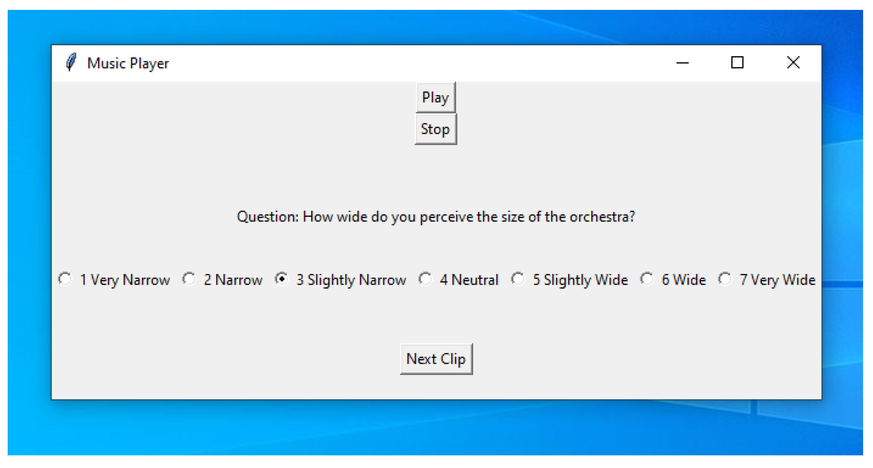
Figure 2.
Signal workflow for RIR measurement.
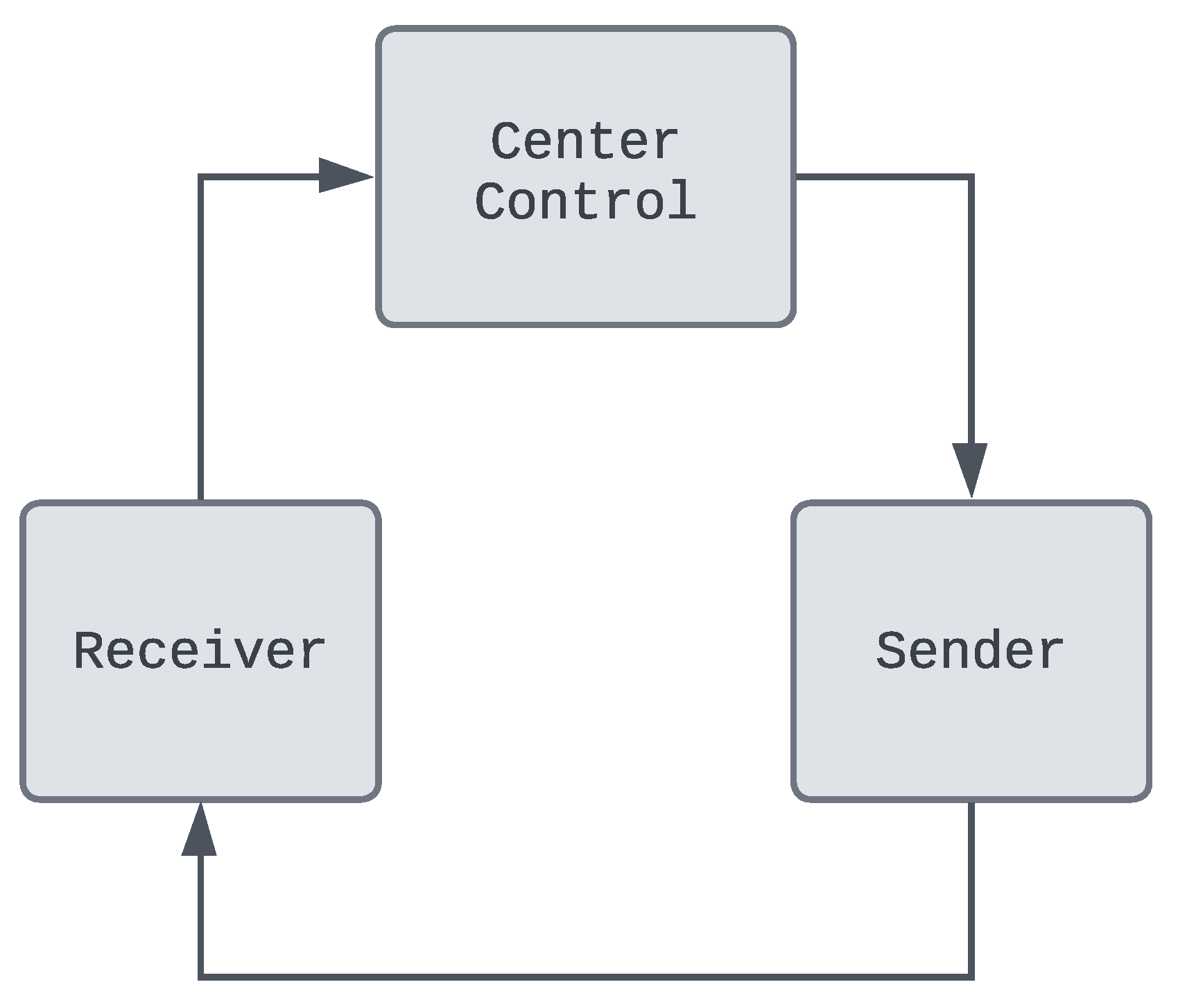
Figure 3.
Omni and figure-8 polar patterns. (Left: . Right: .)
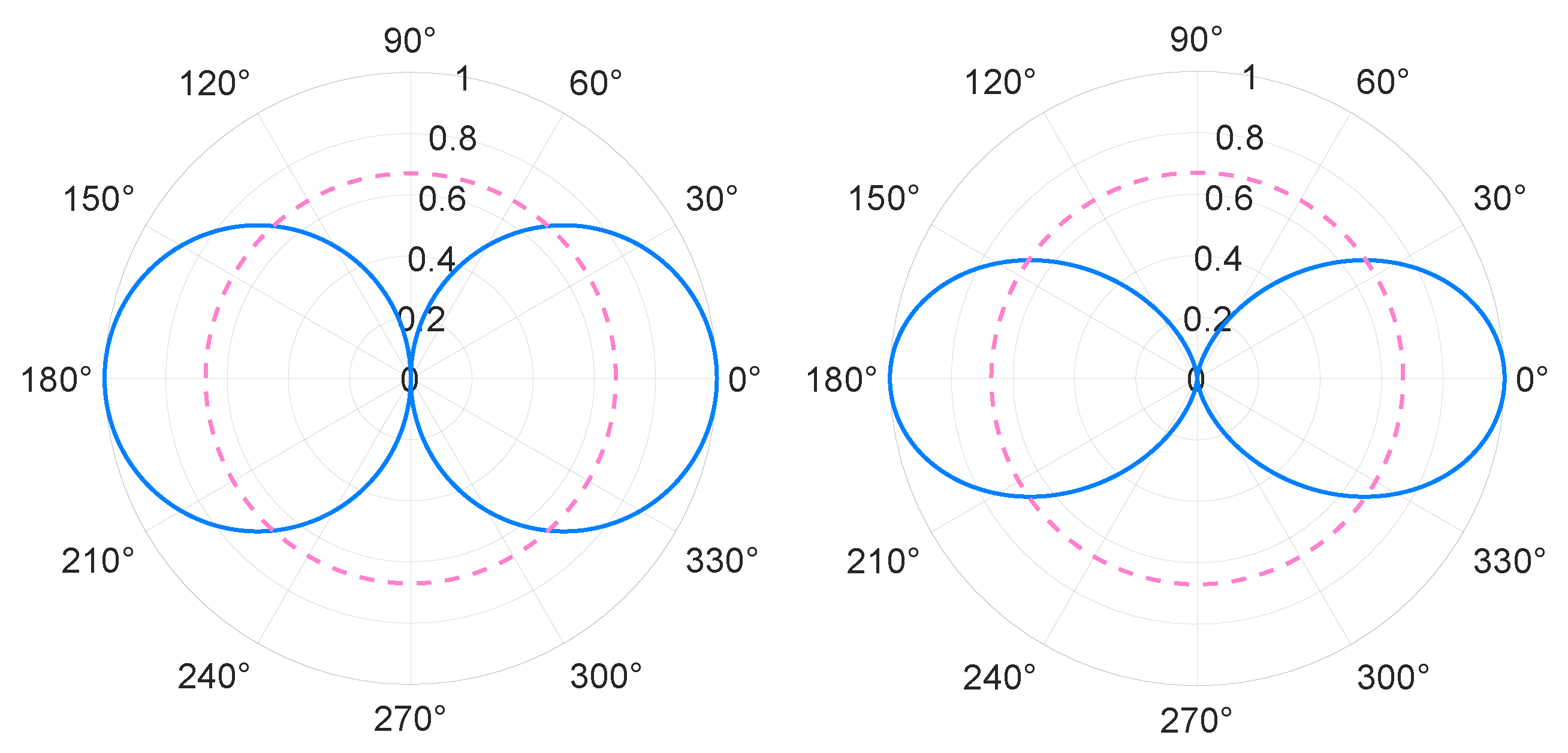
Figure 4.
Seating chart of EMPAC concert hall; spatial and spectral scatter plots for vs. EDT, T30, C80, and LF. The selected seats are represented by 4 colors: blue (Seat 1), red (Seat 2), yellow (Seat 3), and purple (Seat 4).
Figure 4.
Seating chart of EMPAC concert hall; spatial and spectral scatter plots for vs. EDT, T30, C80, and LF. The selected seats are represented by 4 colors: blue (Seat 1), red (Seat 2), yellow (Seat 3), and purple (Seat 4).
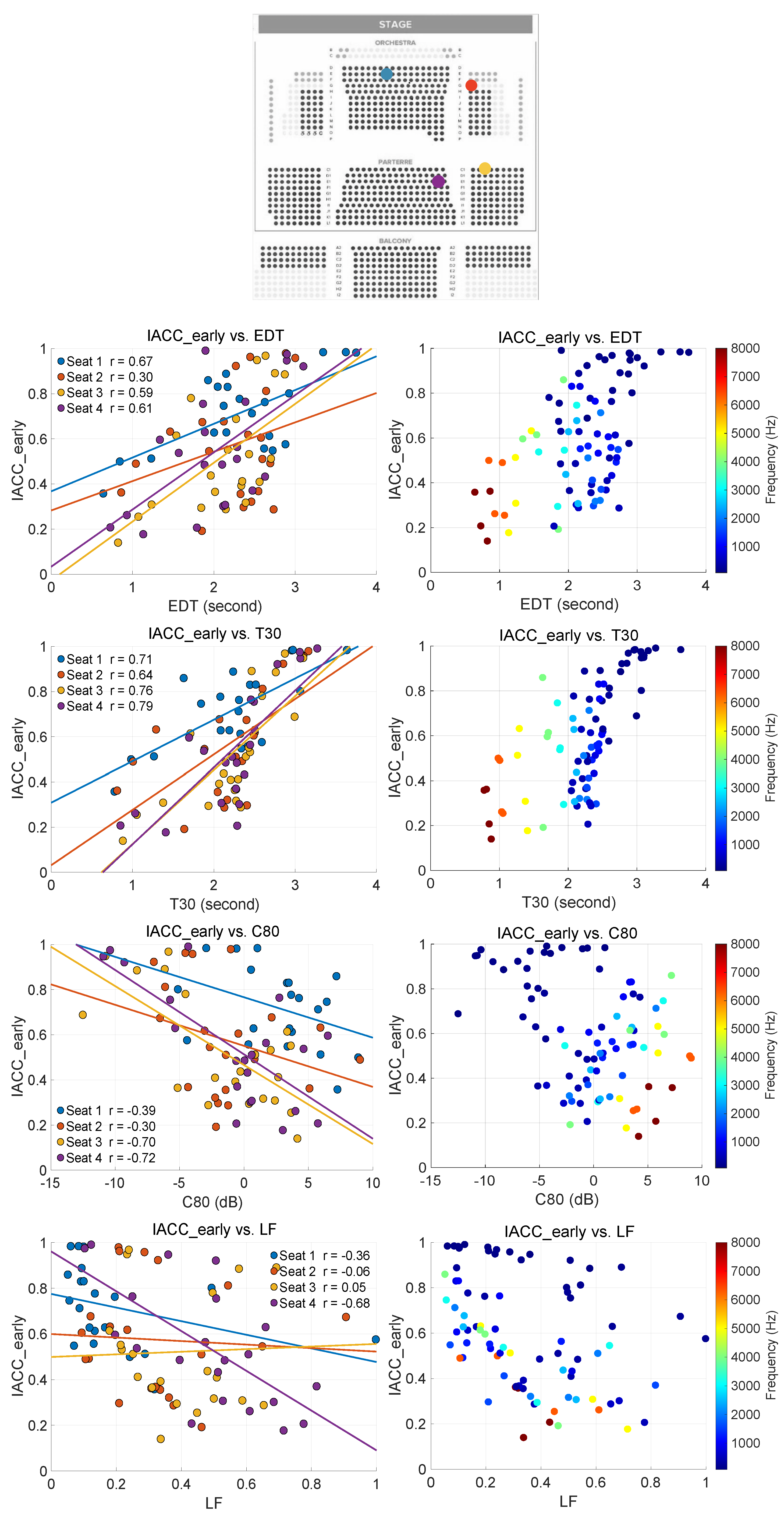
Figure 5.
Measurement results for 14 parameters and energy decay curves with reverberation time line fits.
Figure 5.
Measurement results for 14 parameters and energy decay curves with reverberation time line fits.
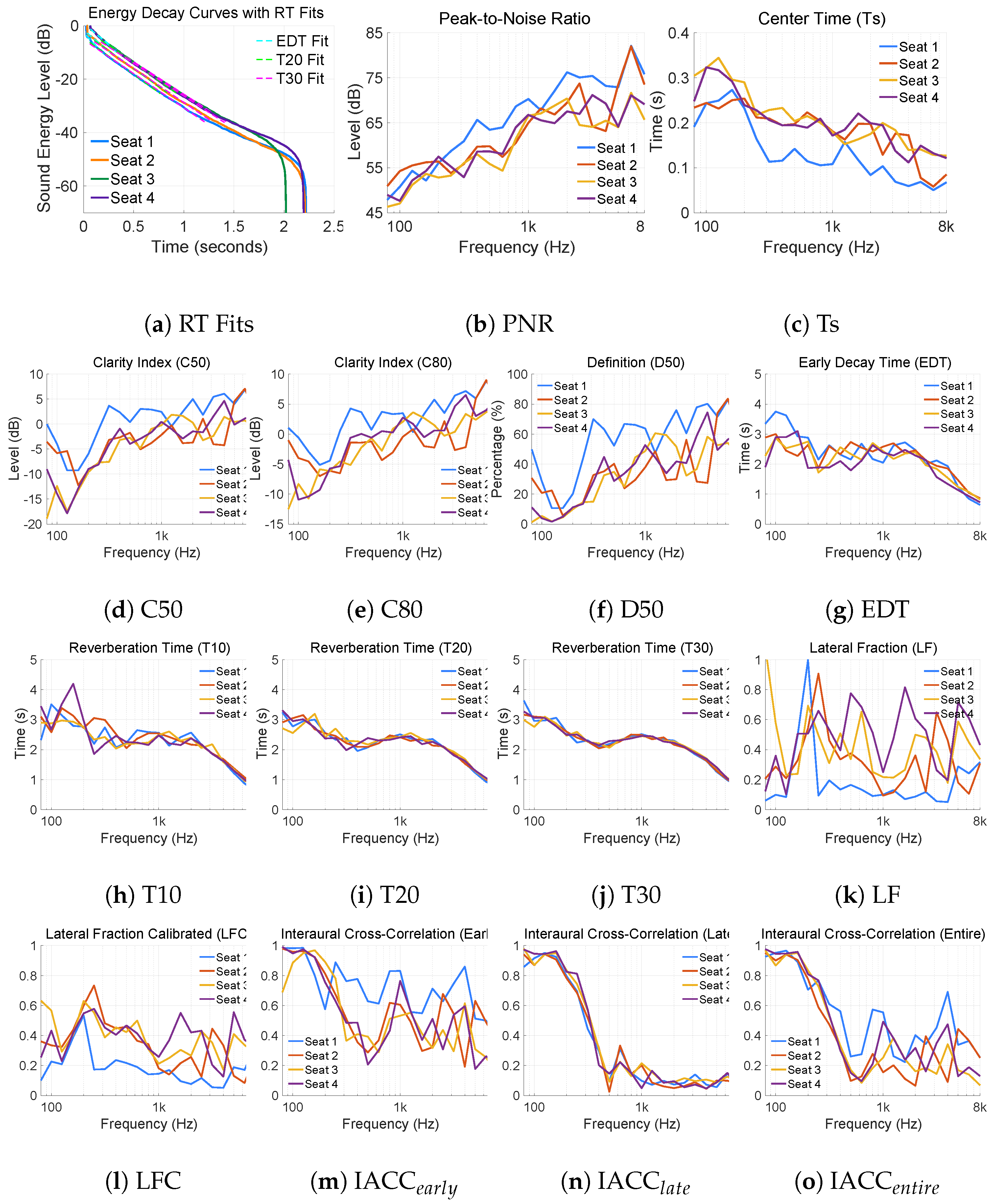

Table 1.
Decay ranges in decibels corresponding to early decay time (EDT) and reverberation time estimations (T10, T20, T30).
Table 1.
Decay ranges in decibels corresponding to early decay time (EDT) and reverberation time estimations (T10, T20, T30).
| EDT | to |
|---|---|
| T10 | to |
| T20 | to |
| T30 | to |
Table 2.
Broadband parameter values per seat.
| Parameter | Seat 1 | Seat 2 | Seat 3 | Seat 4 |
|---|---|---|---|---|
| PNR (dB) | 76.34 | 70.67 | 64.53 | 68.73 |
| C50 (dB) | 4.67 | 2.33 | -0.97 | -0.43 |
| C80 (dB) | 6.01 | 3.58 | 1.22 | 1.81 |
| D50 (%) | 75 | 63 | 44 | 48 |
| Ts (s) | 0.08 | 0.11 | 0.18 | 0.17 |
| EDT (s) | 1.51 | 1.91 | 2.00 | 1.80 |
| T10 (s) | 1.98 | 2.08 | 2.22 | 2.19 |
| T20 (s) | 2.21 | 2.24 | 2.34 | 2.29 |
| T30 (s) | 2.35 | 2.36 | 2.48 | 2.45 |
| LF | 0.16 | 0.16 | 0.35 | 0.45 |
| LFC | 0.14 | 0.14 | 0.31 | 0.33 |
| IACCearly | 0.50 | 0.41 | 0.34 | 0.38 |
| IACClate | 0.13 | 0.13 | 0.18 | 0.19 |
| IACCentire | 0.36 | 0.29 | 0.24 | 0.29 |
Table 3.
Correlation results between mean ASW ratings and spatial parameters for loudspeaker and headphone reproduction conditions.
Table 3.
Correlation results between mean ASW ratings and spatial parameters for loudspeaker and headphone reproduction conditions.
| Condition | ASW vs. IACCearly | ASW vs. LF |
|---|---|---|
| Loudspeaker | ||
| Headphone |
Disclaimer/Publisher’s Note: The statements, opinions and data contained in all publications are solely those of the individual author(s) and contributor(s) and not of MDPI and/or the editor(s). MDPI and/or the editor(s) disclaim responsibility for any injury to people or property resulting from any ideas, methods, instructions or products referred to in the content. |
© 2026 by the authors. Licensee MDPI, Basel, Switzerland. This article is an open access article distributed under the terms and conditions of the Creative Commons Attribution (CC BY) license (http://creativecommons.org/licenses/by/4.0/).
Copyright: This open access article is published under a Creative Commons CC BY 4.0 license, which permit the free download, distribution, and reuse, provided that the author and preprint are cited in any reuse.


