
Submitted:
15 January 2025
Posted:
16 January 2025
You are already at the latest version
Abstract
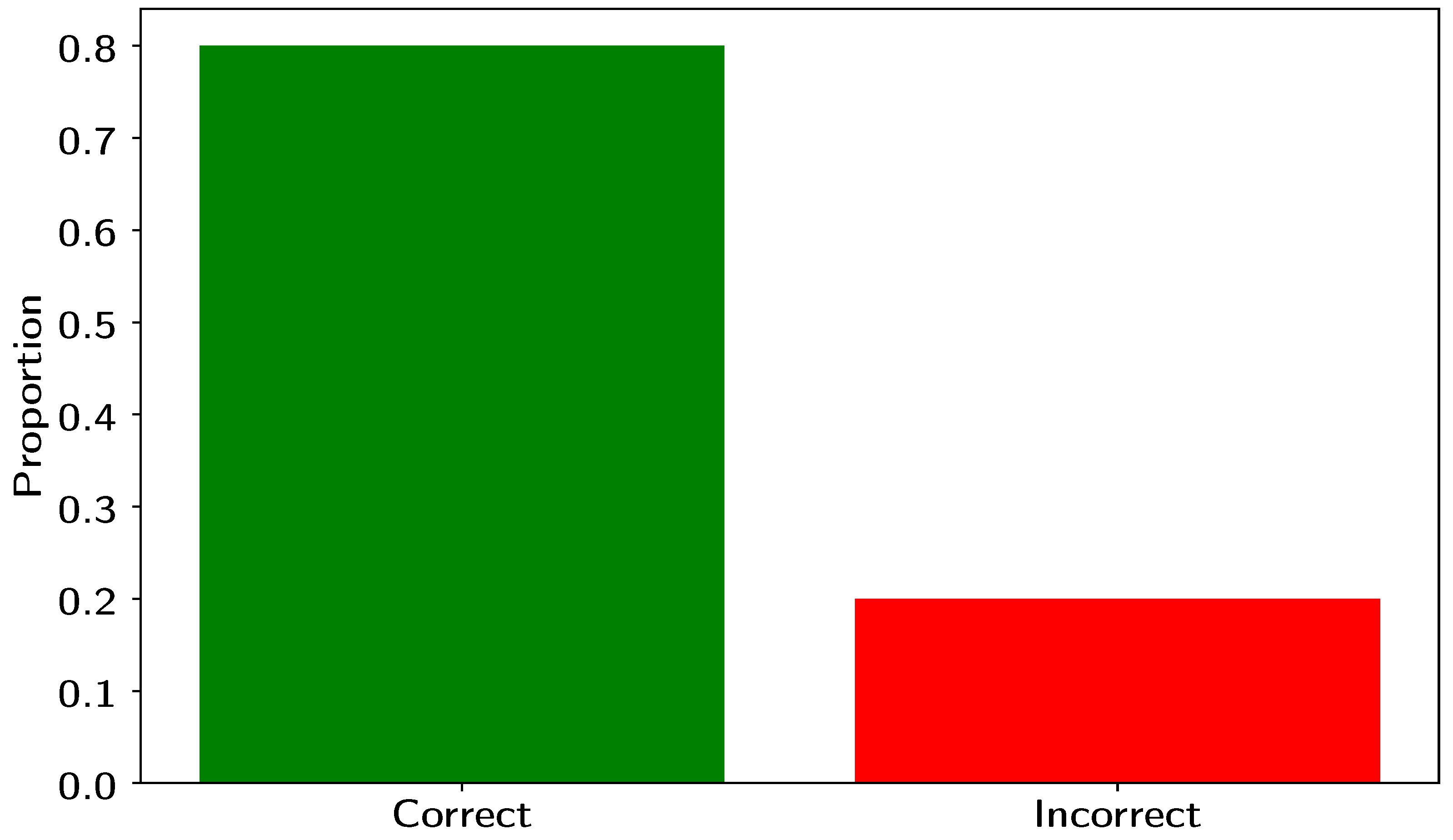
This paper presents a comprehensive evaluation using a Z-test to assess the 1 effectiveness of an adaptive Least Mean Squares (LMS) filter driven by the Steepest Descent 2 Method (SDM). The study utilizes a male voice recording, captured in a controlled studio 3 environment, to which persistent Gaussian noise was intentionally introduced, simulating 4 real-world interference. All signal processing methods were implemented accordingly 5 in MATLAB. The adaptive filter demonstrated a significant improvement of 20 dB in 6 Signal-to-Noise Ratio (SNR) following the initial optimization of the filter parameter μ. 7 To further assess the LMS filter’s performance, an empirical experiment was conducted 8 with 30 young adults, aged between 20 and 30 years, who were tasked with qualitatively 9 distinguishing between the clean and noise-corrupted signals (blind test). The quantitative 10 analysis and statistical evaluation of the participants’ responses revealed that a significant 11 majority, specifically 80%, were able to reliably identify the noise-affected and filtered 12 signals. This outcome highlights the LMS filter’s potential—despite the slow convergence of 13 the SDM—for enhancing signal clarity in noise-contaminated environments, thus validating 14 its practical application in speech processing and noise reduction
Keywords:
1. Introduction
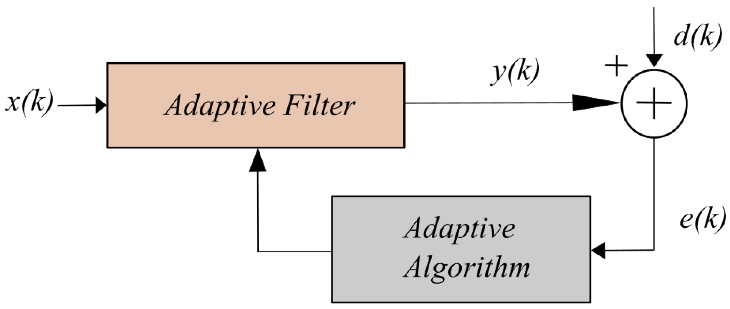
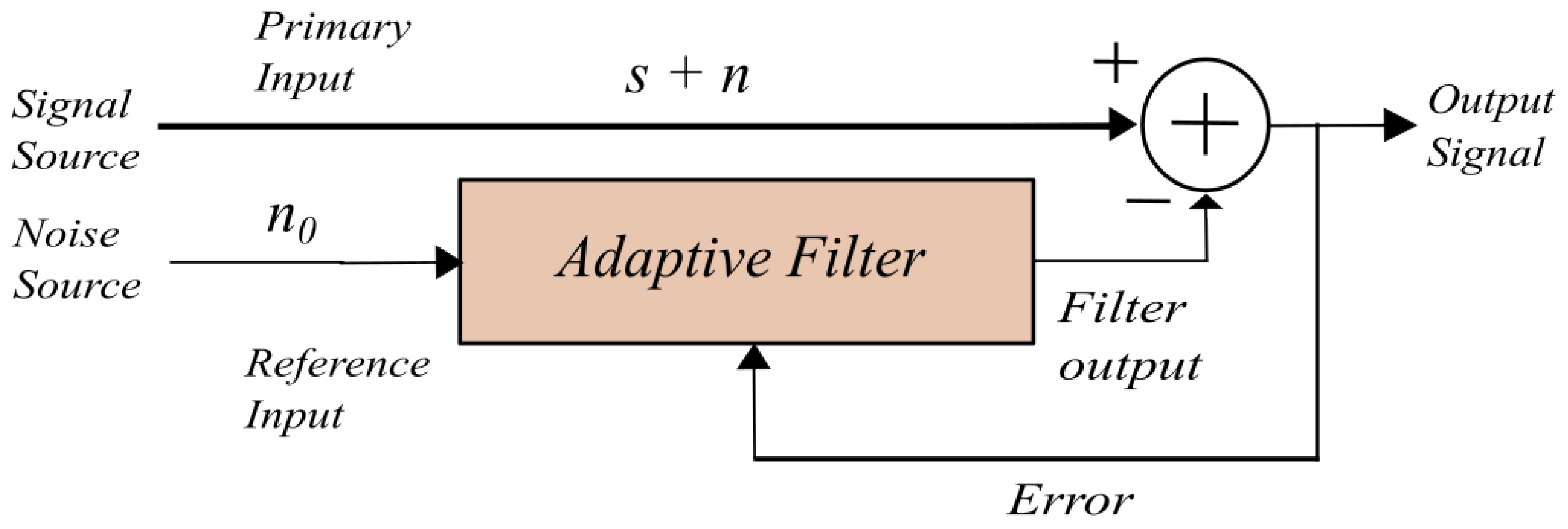
- Gaussian Noise: often referred to as "white noise," is characterized by a flat spectral density across the frequency spectrum. This type of noise is particularly useful for simulating real-world conditions, as it encompasses all frequencies with equal intensity. The power spectral density of Gaussian noise is uniform, which means that it contains equal amounts of noise power across all frequencies. In practice, this makes it a valuable tool for testing the performance of noise cancelation algorithms. The term "Gaussian" refers to the statistical distribution of the noise, where the amplitude of the noise follows a normal (Gaussian) distribution. This is in contrast to other types of noise, such as impulsive noise, which is characterized by brief, high-intensity spikes. Gaussian noise is often used in simulations as it represents a wide variety of natural noise sources, from thermal noise in electronic components to environmental noise in real-world settings. Its use in this research provides a controlled yet representative form of interference to evaluate the effectiveness of the LMS filter in improving signal clarity and noise reduction. Why LMS? The Least Mean Squares (LMS) algorithm provides an adaptive filter algorithm that minimizes the difference between the desired signal and the filtered signal. By iterative adjustment of the filter coefficients, LMS is able to optimize the filter in real-time, making it an ideal solution for adaptive noise cancellation applications. The basic operation of LMS relies on the principle of gradient descent, where the filter coefficients are updated in the direction of the steepest decrease in the error signal, thus minimizing the Mean Squared Error (MSE) between the desired and actual outputs. LMS is computationally efficient and straightforward to implement, making it particularly useful in applications with limited computational resources. Despite its relatively slow convergence rate, especially compared to other adaptive algorithms such as recursive least squares (RLS), LMS remains widely adopted due to its simplicity and efficiency [21]. In this study, the LMS filter is driven by the Steepest Descent Method (SDM), a foundational optimization technique that iteratively adjusts parameters to minimize an objective function, in this case, the MSE. Although SDM can converge slower than other optimization methods, its effectiveness and practicality in real-time systems make it an attractive choice for active noise cancellation systems [13,22,23]. Optimization of LMS filters is especially useful for applications that involve persistent noise. For example, in audio recordings, where unwanted noise (often added in an additive manner) needs to be reduced or eliminated, LMS can be employed to dynamically adjust its coefficients(see Figure 1) to match the noise profile and filter it out. The filter adaptation to noise is determined by the parameter , which controls the rate of adaptation. Proper tuning of is crucial, as a small value may result in slow convergence, while a large value can cause instability in the filter.
2. Materials and Methods
- Least Mean Squares (LMS) Algorithm:
- Signal Processing:
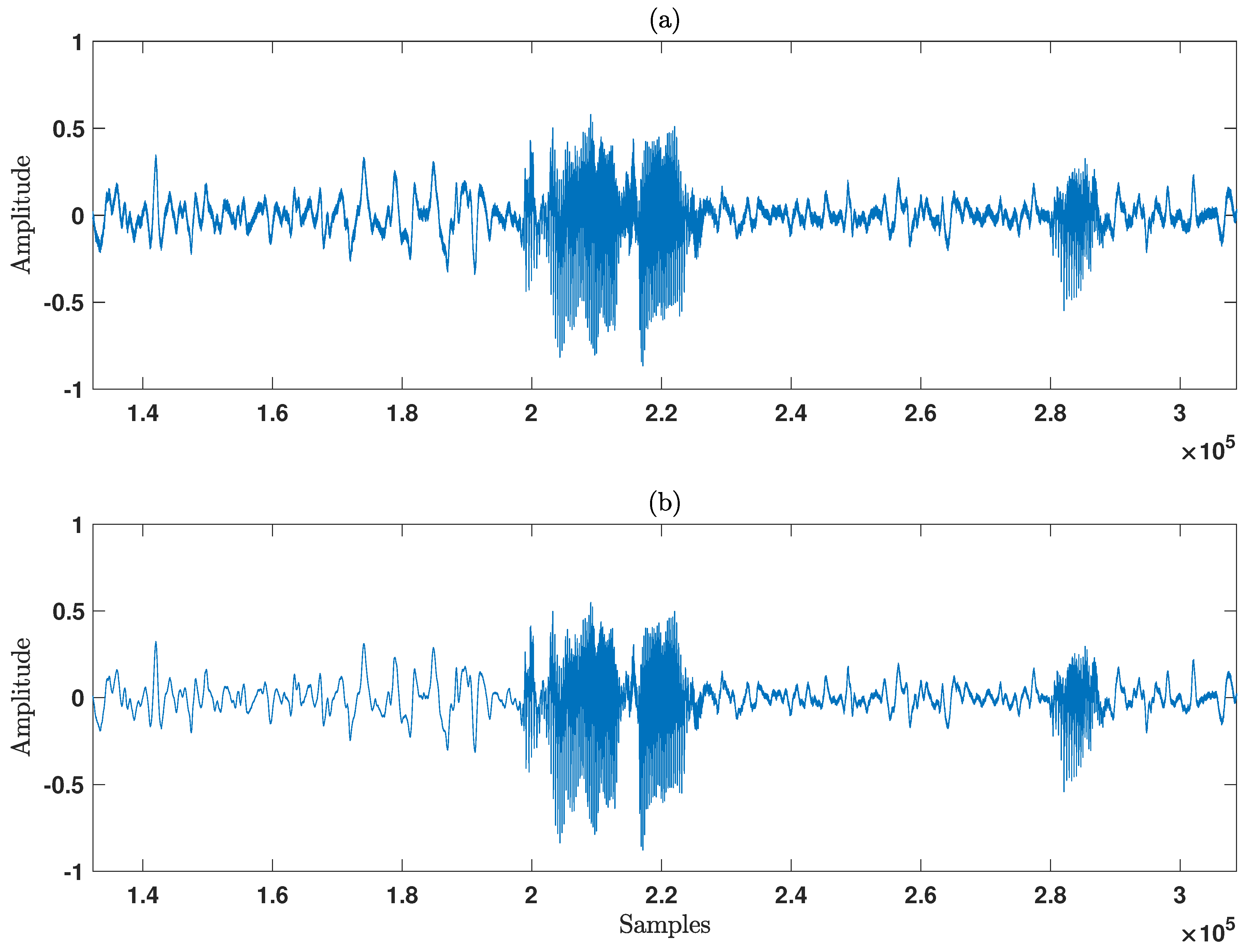
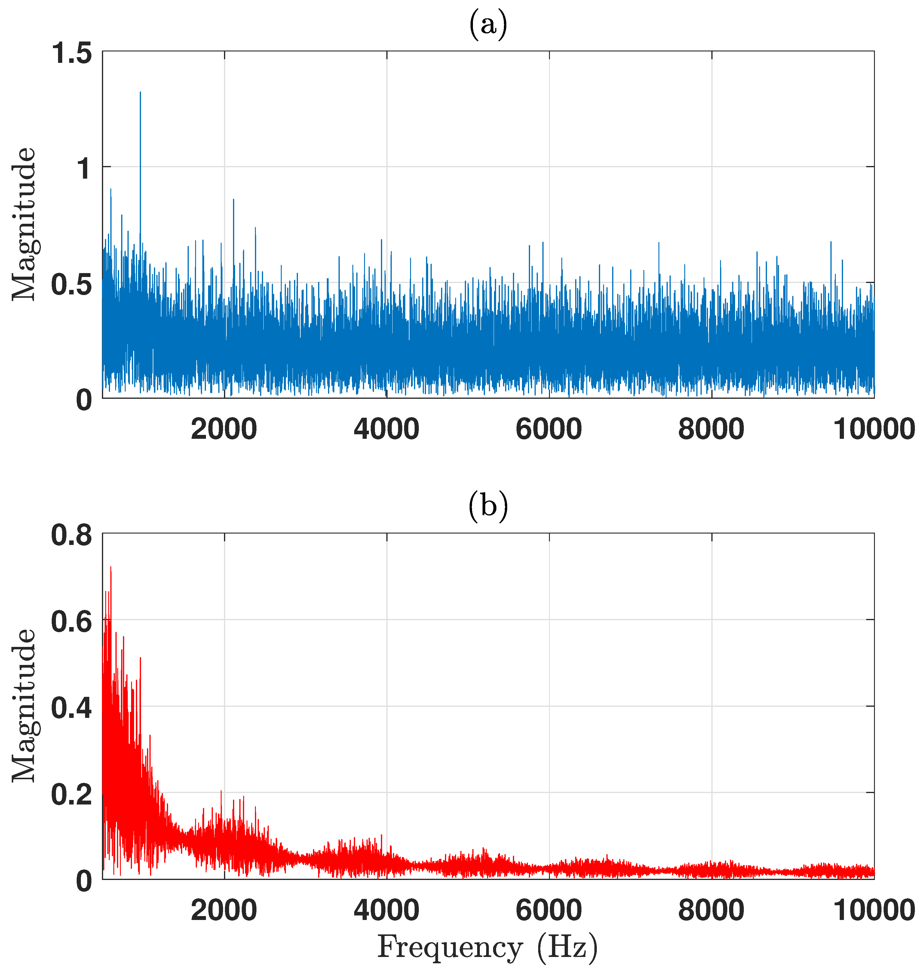
- Signal processing was performed using the Least Mean Squares (LMS) algorithm implemented in MATLAB. The algorithm was applied to a male voice recording that had been corrupted with Gaussian noise, resulting in a signal with a degraded Signal-to-Noise Ratio, corrupted signal level was 10 dB SNR. The noise reduction achieved by the LMS filter improved the SNR by 20 dB (for the detailed equation used to calculate the SNR improvement, please refer to the appendix). To visualize the effects of the noise reduction, the Fast Fourier Transform (FFT) of both the corrupted signal and the filtered signal were computed.
- Blind Test Design:
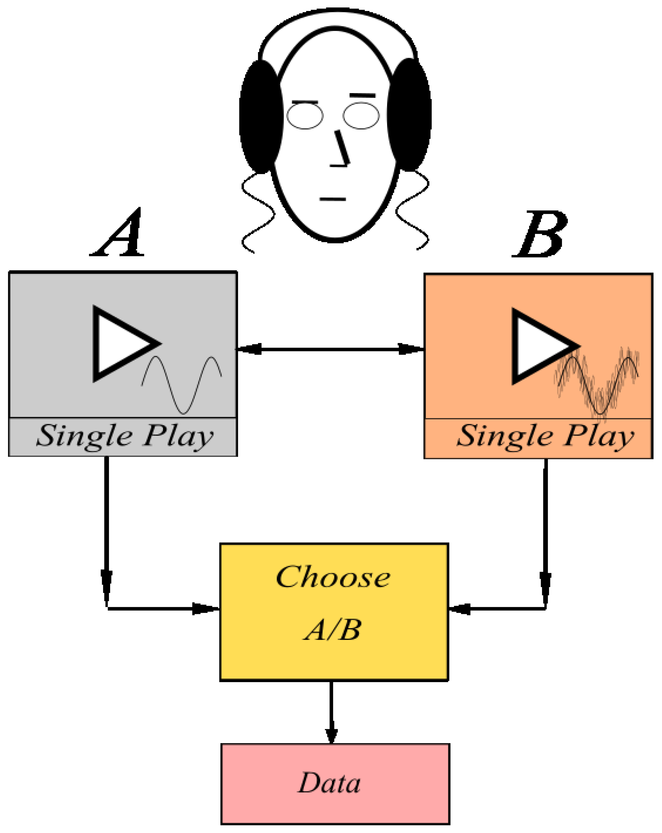
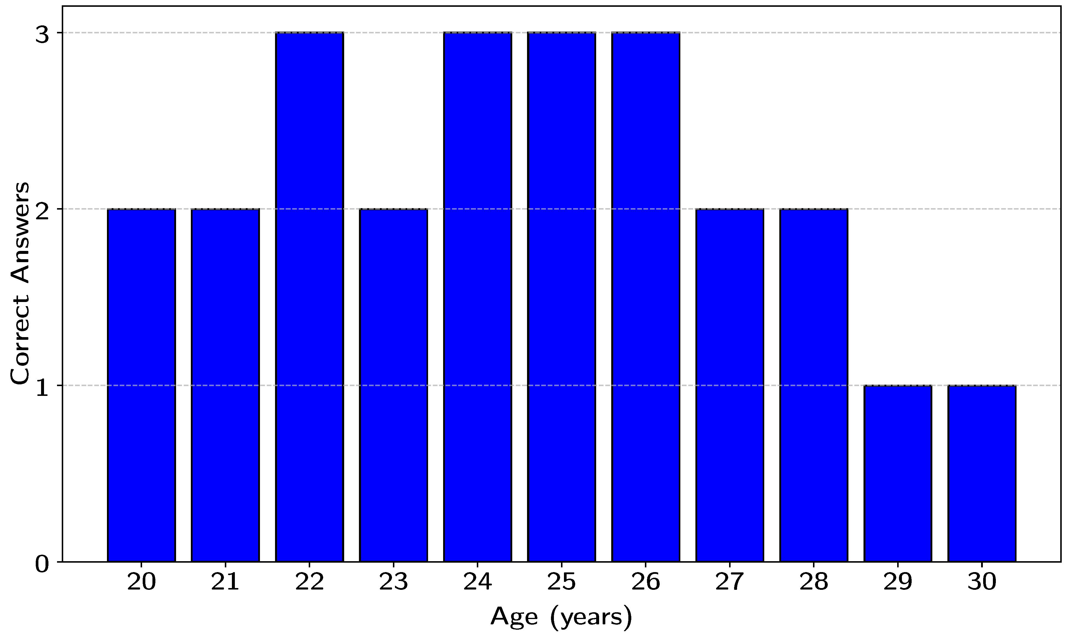
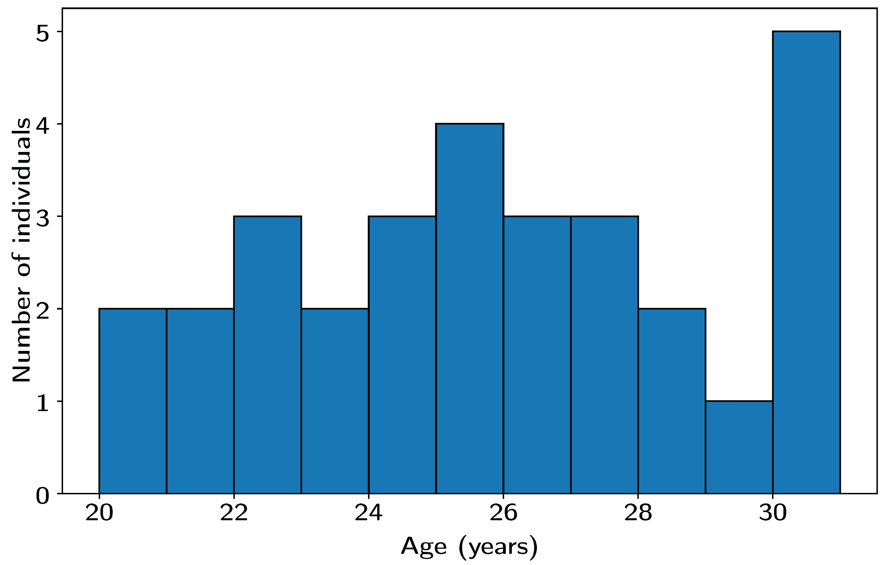
- To assess the effectiveness of the LMS filter on human perception, a blind test was designed. A total of 30 young adult participants, aged between 20 and 30 years, were recruited for the study. Each participant was provided with a pair of earphones and a mobile phone to listen to the audio signals. They were presented with two signals, labeled A and B, and were asked to identify which signal had undergone noise reduction. The order of presentation was randomized, and participants were unaware of which signal was the filtered version, ensuring the integrity of the blind test. Their responses were recorded for later analysis. The test was conducted in a controlled environment inside a soundproof recording booth to prevent external noise interference. This setting ensured that the only noise present was the Gaussian noise initially introduced into the signal. A schematic of the experimental setup is presented in Figure 3, detailing the experiment design.
- Data Collection:
- The responses of the participants were categorized into two options: "A" for the noise-reduced signal and "B" for the noise-corrupted signal. The frequency of correct and incorrect identification was recorded for each participant. The results were then compiled and analyzed to assess the overall effectiveness of the LMS filter in improving the perception of the signal. For all collected data refer to Appendix A
- Statistical Analysis:
- The data obtained from the blind test were analyzed using a Z-test for proportions to make statistical inferences regarding the effectiveness of the noise reduction. This test was applied to compare the proportion of correct identifications of the filtered signal with the proportion expected by chance (50%). A significance level of 0.05 was used to determine whether the LMS filter produced a statistically significant improvement in the participants’ ability to correctly identify the noise-reduced signal. In this study, the effectiveness of the LMS filter in improving the perception of the noise-reduced signal was analyzed using a Z-test for proportions. The Z test for proportions is a statistical test used to determine whether the proportion of correct identifications is significantly different from the proportion hypothesized of 50%(ie, random guessing in the absence of noise reduction). The null hypothesis () states that the proportion of correct identifications is equal to the hypothesized value, while the alternative hypothesis () posits that the proportion is greater than the hypothesized value [29] (i.e., the LMS filter improves the perception of the signal).
- Hypotheses:
- Null Hypothesis (): The proportion of correct identifications, p, is equal to 0.5 (i.e., no improvement, random guessing).
- Alternative Hypothesis (): The proportion of correct identifications, p, is greater than 0.5 (i.e., the filter improves the perception). The Z-test statistic for proportions is calculated using the formula:Where:
- Confidence Interval
- In addition to the Z-test, the 95% confidence interval for the true proportion of correct identifications is calculated to provide a range of plausible values for the population proportion. This confidence interval is given by the following equation:is the confidence interval for the proportion.
- is the observed proportion of correct identifications.
- is the Z-value for a 95% confidence level (typically 1.96)[29].
- n is the sample size (30 participants in this study). If the calculated Z-value exceeds the critical value (1.96 for a 95% confidence level), the null hypothesis is rejected, indicating that the LMS filter significantly improved the perception of the signal. The confidence interval provides an estimate of the range in which the true proportion of correct identifications is likely to fall, with 95% certainty.
3. Results
- Statistical Analysis and Interpretation.
- A Z-test for proportions was conducted to assess the effectiveness of the LMS filter in enhancing the ability of participants to correctly identify the filtered signal as compared to the corrupted signal. The test was designed to determine whether the proportion of correct responses, observed in the experiment, was significantly greater than what would be expected by random guessing.
- Test Results:
- Statistical Significance:
-
The null hypothesis () posited that the observed proportion of correct responses is equal to 0.5, representing random guessing. This can be expressed as:The alternative hypothesis () stated that the observed proportion is greater than 0.5, implying that the LMS filter had a significant effect on improving the perception of the filtered signal:
- Confidence Interval:
- The 95% Confidence Interval for the true proportion of correct responses was calculated to be:(0.6569, 0.9431).This interval does not include 0.5, further supporting the conclusion that the proportion of correct responses is significantly higher than expected by chance. This suggests that the LMS filter had a positive effect on the ability of participants to distinguish the filtered signal from the noisy one.
4. Discussion
5. Conclusions
Appendix A

| Subject | Age | A Signal | B Signal | Signal Selected |
|---|---|---|---|---|
| P1 | 20 | Filtered | Corrupted | A |
| P2 | 20 | Filtered | Corrupted | A |
| P3 | 20 | Filtered | Corrupted | A |
| P4 | 21 | Corrupted | Filtered | B |
| P5 | 21 | Filtered | Corrupted | A |
| P6 | 22 | Corrupted | Filtered | B |
| P7 | 22 | Filtered | Corrupted | A |
| P8 | 22 | Corrupted | Filtered | B |
| P9 | 22 | Corrupted | Filtered | B |
| P10 | 24 | Corrupted | Filtered | B |
| P11 | 24 | Filtered | Corrupted | A |
| P12 | 24 | Filtered | Corrupted | A |
| P13 | 25 | Filtered | Corrupted | A |
| P14 | 25 | Filtered | Corrupted | B |
| P15 | 25 | Corrupted | Filtered | B |
| P16 | 25 | Corrupted | Filtered | B |
| P17 | 26 | Corrupted | Filtered | B |
| P18 | 26 | Filtered | Corrupted | A |
| P19 | 26 | Corrupted | Filtered | B |
| P20 | 27 | Filtered | Corrupted | A |
| P21 | 27 | Corrupted | Filtered | A |
| P22 | 28 | Corrupted | Filtered | B |
| P23 | 28 | Filtered | Corrupted | A |
| P24 | 28 | Corrupted | Filtered | B |
| P25 | 29 | Filtered | Corrupted | B |
| P26 | 30 | Corrupted | Filtered | A |
| P27 | 30 | Corrupted | Filtered | A |
| P28 | 30 | Corrupted | Filtered | A |
| P29 | 30 | Filtered | Corrupted | B |
| P30 | 30 | Filtered | Corrupted | B |
Appendix B
Mathematical Derivation of the Steepest Descent Method
Objective Function to Minimize
Gradient of the Function
Update Rule
- is the vector of parameters at iteration k.
- is the step size (learning rate), which determines how much the parameters should change at each iteration.
- is the gradient of the function at iteration k.
In the Context of the LMS Filter
- is the desired signal at time k.
- is the vector of filter coefficients.
- is the input vector (features or signals) at time k.
Summary of the Mathematical Development
- Objective Function: The error function is defined, which we aim to minimize.
- Gradient of the Function: The gradient of the error function is computed, indicating the direction of steepest increase.
- Update Rule: The filter coefficients are updated in the opposite direction of the gradient, applying a step size to control the speed of convergence.
Appendix C
Appendix C.1. MATLAB script for LMS and SDM Implmentation
References
- Agnew, J. Audible circuit noise in hearing aid amplifiers. The Journal of the Acoustical Society of America 1997, 102, 2793–2799.
- Keizer, G. The unwanted sound of everything we want: A book about noise; PublicAffairs, 2010.
- Kim, S.; Arzac, S.; Dokic, N.; Donnelly, J.; Genser, N.; Nortwich, K.; Rooney, A. Cortical and Subjective Measures of Individual Noise Tolerance Predict Hearing Outcomes with Varying Noise Reduction Strength. Applied Sciences (2076-3417) 2024, 14.
- Ding, T.; Yan, A.; Liu, K. What is noise-induced hearing loss? British Journal of Hospital Medicine 2019, 80, 525–529.
- Mueller, B.J.; Liebl, A.; Herget, N.; Kohler, D.; Leistner, P. Using active noise-cancelling headphones in open-plan offices: No influence on cognitive performance but improvement of perceived privacy and acoustic environment. Frontiers in Built Environment 2022, 8, 962462.
- Alvarsson, J.J.; Wiens, S.; Nilsson, M.E. Stress recovery during exposure to nature sound and environmental noise. International journal of environmental research and public health 2010, 7, 1036–1046.
- Münzel, T.; Sørensen, M.; Schmidt, F.; Schmidt, E.; Steven, S.; Kröller-Schön, S.; Daiber, A. The adverse effects of environmental noise exposure on oxidative stress and cardiovascular risk. Antioxidants & redox signaling 2018, 28, 873–908.
- Frühholz, S.; Belin, P. The science of voice perception; Vol. 1, Oxford University Press Oxford, 2018.
- Wang, X.; Xu, L. Speech perception in noise: Masking and unmasking. Journal of Otology 2021, 16, 109–119.
- Masullo, M.; Yamauchi, K.; Dan, M.; Cioffi, F.; Maffei, L. Influence of Infotainment-System Audio Cues on the Sound Quality Perception Onboard Electric Vehicles in the Presence of Air-Conditioning Noise. In Proceedings of the Acoustics. MDPI, 2024, Vol. 7, p. 1.
- Ballou, G. Handbook for sound engineers; Taylor & Francis, 2013.
- Cheng, H.L.; Han, J.Y.; Chu, Y.C.; Cheng, Y.F.; Lin, C.M.; Chiang, M.C.; Wu, S.L.; Lai, Y.H.; Liao, W.H. Evaluating the hearing screening effectiveness of active noise cancellation technology among young adults: A pilot study. Journal of the Chinese Medical Association 2023, 86, 105–112.
- Zacharov, N.; Ramsgaard, J.; Le Ray, G.; Jørgensen, C.V. The multidimensional characterization of active noise cancelation headphone perception. In Proceedings of the 2010 Second International Workshop on Quality of Multimedia Experience (QoMEX). IEEE, 2010, pp. 130–135.
- Jurado, C.; Gallegos, P.; Gordillo, D.; Moore, B.C. The detailed shapes of equal-loudness-level contours at low frequencies. The Journal of the Acoustical Society of America 2017, 142, 3821–3832.
- Rasetshwane, D.M.; Trevino, A.C.; Gombert, J.N.; Liebig-Trehearn, L.; Kopun, J.G.; Jesteadt, W.; Neely, S.T.; Gorga, M.P. Categorical loudness scaling and equal-loudness contours in listeners with normal hearing and hearing loss. The Journal of the Acoustical Society of America 2015, 137, 1899–1913.
- Glasberg, B.R.; Moore, B.C. Prediction of absolute thresholds and equal-loudness contours using a modified loudness model. The Journal of the Acoustical Society of America 2006, 120, 585–588.
- Motlagh Zadeh, L.; Silbert, N.H.; Sternasty, K.; Swanepoel, D.W.; Hunter, L.L.; Moore, D.R. Extended high-frequency hearing enhances speech perception in noise. Proceedings of the National Academy of Sciences 2019, 116, 23753–23759.
- Kreiman, J.; Gerratt, B.R. Perceptual interaction of the harmonic source and noise in voice. The Journal of the Acoustical Society of America 2012, 131, 492–500.
- Titze, I.R.; Palaparthi, A. Vocal loudness variation with spectral slope. Journal of Speech, Language, and Hearing Research 2020, 63, 74–82.
- Tait, B.L. Applied Fletcher-Munson curve algorithm for improved voice recognition. International Journal of Electronic Security and Digital Forensics 7 2012, 4, 178–186.
- Chen, Y.; Gu, Y.; Hero, A.O. Regularized least-mean-square algorithms. arXiv preprint arXiv:1012.5066 2010.
- McKenzie, T.; Armstrong, C.; Ward, L.; Murphy, D.T.; Kearney, G. Predicting the colouration between binaural signals. Applied Sciences 2022, 12, 2441.
- Ang, L.Y.L.; Koh, Y.K.; Lee, H.P. The performance of active noise-canceling headphones in different noise environments. Applied Acoustics 2017, 122, 16–22.
- Hayes, M.H. Statistical Digital Signal Processing and Modeling; John Wiley & Sons, 1996.
- Lee, J.H.; Ooi, L.E.; Ko, Y.H.; Teoh, C.Y. Simulation for noise cancellation using LMS adaptive filter. In Proceedings of the IOP Conference Series: Materials Science and Engineering. IOP Publishing, 2017, Vol. 211, p. 012003.
- Ferdouse, L.; Akhter, N.; Nipa, T.H.; Jaigirdar, F.T. Simulation and performance analysis of adaptive filtering algorithms in noise cancellation. arXiv preprint arXiv:1104.1962 2011.
- He, Y.; He, H.; Li, L.; Wu, Y.; Pan, H. The applications and simulation of adaptive filter in noise canceling. In Proceedings of the 2008 International conference on computer science and software engineering. IEEE, 2008, Vol. 4, pp. 1–4.
- Foley, J.; Boland, F. Comparison between steepest descent and LMS algorithms in adaptive filters. In Proceedings of the IEE Proceedings F (Communications, Radar and Signal Processing). IET, 1987, Vol. 134, pp. 283–289.
- Martagón, V.L.; et al. Bioestadística; Editorial El Manual Moderno, 2014.
- Yoshizawa, T.; Hirobayashi, S.; Misawa, T. Noise reduction for periodic signals using high-resolution frequency analysis. EURASIP Journal on Audio, Speech, and Music Processing 2011, 2011, 1–19.
- Suzuki, Y.; Takeshima, H.; Kurakata, K. Revision of ISO 226" Normal Equal-Loudness-Level Contours" from 2003 to 2023 edition: The background and results. Acoustical Science and Technology 2024, 45, 1–8.
- Stevens, S. Calculation of the loudness of complex noise. The Journal of the Acoustical Society of America 1956, 28, 807–832.
- Narayan, S.S.; Peterson, A. Frequency domain least-mean-square algorithm. Proceedings of the IEEE 1981, 69, 124–126.
- Rao, H.I.; Farhang-Boroujeny, B. Fast LMS/Newton algorithms for stereophonic acoustic echo cancelation. IEEE Transactions on Signal Processing 2009, 57, 2919–2930.
- Carlile, S.; Hyams, S.; Delaney, S. Systematic distortions of auditory space perception following prolonged exposure to broadband noise. The Journal of the Acoustical Society of America 2001, 110, 416–424.
- Srivastava, D.; Narayanan, V.; Singh, B.; Verma, A. A Novel Steepest Descent Least Mean Square Control for Smooth Mode Transfer of a Single-Stage SPVA-BES Hybrid Microgrid. IEEE Transactions on Industry Applications 2024.
- Schäffer, B.; Pieren, R.; Schlittmeier, S.J.; Brink, M. Effects of different spectral shapes and amplitude modulation of broadband noise on annoyance reactions in a controlled listening experiment. International journal of environmental research and public health 2018, 15, 1029.
Disclaimer/Publisher’s Note: The statements, opinions and data contained in all publications are solely those of the individual author(s) and contributor(s) and not of MDPI and/or the editor(s). MDPI and/or the editor(s) disclaim responsibility for any injury to people or property resulting from any ideas, methods, instructions or products referred to in the content. |
© 2025 by the authors. Licensee MDPI, Basel, Switzerland. This article is an open access article distributed under the terms and conditions of the Creative Commons Attribution (CC BY) license (http://creativecommons.org/licenses/by/4.0/).


