Submitted:
05 January 2026
Posted:
16 January 2026
You are already at the latest version
Abstract
We provide generalizations of the conventional logistic population dynamics models suitable for periodic breeders, such as migratory birds, occupying varied habitats during the breeding cycle. These models require separate density dependencies for the birth and death rates, which may be habitat specific. Some analytical functional forms for the density dependencies are discussed where the population controlling mechanisms are each characterized by a distinct carrying capacity and saturation power. Multiple mechanisms might be operative simultaneously with the smallest carrying capacity usually dominating, but subject to influence from the others. We compare the dynamics and applicability for corresponding continuous differential and discrete difference population models. Generally, the differential models are stable, but exhibit repetitive seasonal variations for periodic breeders. The inherent delays in the discrete models may yield instabilities for large birth rates, as is known for single habitats, and may lead to significant discrepancies from the differential models for periodic breeders. The discrete models are also applicable to the life cycles of metamorphic and spawning species with non-overlapping generations. Threshold effects are also considered.
Keywords:
population dynamics
; density dependence
; sequential habitats
; carrying capacity
; saturation mechanisms
; threshold effects
; migratory birds
; metamorphic species
1. Introduction
Fretwell (1972) has discussed many of the factors influencing the selection and dispersal among various habitats for populations in seasonal environments. A number of studies of neotropical migrant birds, such as reviewed by Rappole et al. (1983), Rappole (1995) and Sherry and Holmes (1995), have suggested that limited and deteriorating resources in the wintering habitats have contributed to population declines for several species. Sutherland (1996) has provided an estimate of the decline in equilibrium populations from reduction of the breeding or non-breeding habitats based on the density dependencies of the respective birth and death rates. Seasonal population dynamics models addressing the problem of variable habitats are customarily based on the classical logistic differential equation of Verhulst (1845,1847),
describing the density-limited rate of growth of a population. Here, is the population density, N, relative to the carrying capacity, K, of the habitat, and r is the ”intrinsic” growth rate, usually associated with the difference between the birth and death rates, . The factor represents the density dependence of r, moderating otherwise exponential Malthusian growth. This expression has the analytical solution (Pearl 1927, Maynard Smith 1968, Pielou 1969, Acheson 1997),
where is the initial population density. For , this solution starts out with nearly exponential growth, but eventually saturates exactly at the carrying capacity, , exhibiting the well-known ”sigmoidal” shape. Pearl (1927) demonstrated the utility of the logistic curve in fitting the growth of laboratory-cultured yeast, but similar logistic projections of the US population (saturating at ~200 million in year ~2000) from historic census data (Pearl, Reed and Kish 1940) have not been realized. Though extrapolation of any model fit to limited, noisy data is always risky, such failure likely results from inadequacies of the model.
The Verhulst logistic, Equation , is a deterministic, single-species, single-mechanism, single-isolated-habitat, age-independent, spatially-homogeneous, instantaneous-response, first-order density-dependent model. These assumptions may restrict its applicability, and the literature is replete with extensions for statistical fluctuations of the parameters, predator-prey and competitive species interactions, age-specific birth and death rates, spatial diffusion, delayed response, and nonlinear density dependencies (see texts: Lotka 1956, Maynard-Smith 1968, 1974, Pielou 1969, Royama 1992, Krebs 1994, Kot 2001, Caswell 2006, and references therein). In this work, we primarily consider generalizations for multiple habitats and mechanisms encountered by migratory or resident seasonal breeders. We also examine threshold effects and possible instabilities due to the delayed response inherent in substituting discrete difference equations for differential equations, such as Equation . In a companion paper (Pine and Rappole 2008), we discuss the requirements for the validity of overall density-dependent population dynamics models for periodic breeders that exhibit age-structured birth and death rates.
2. Generalized Single-Habitat Logistic Models
The Verhulst logistic model, Equation , has only two parameters, r and K, available to fit data, and K is just a scale factor. For increased flexibility, Richards (1959) and Gilpin and Ayala (1973) introduced an additional ”asymmetry parameter”, p, to the density dependence, in the form, . Herein, we refer to this p parameter as the ”saturation power”, since it affects the abruptness of the population saturation, as shown below. However, this modification, as well as the standard case, may have some difficulties for populations that exceed the carrying capacity because of the negative-going density-dependent factor. In particular, if the birth rate is less than the death rate, then extinction is predicted for , as expected, but anomalous growth occurs for . Indeed, for and , the denominator in Equation vanishes at , leading to a population singularity (Kuno 1991, Royama 1992). For this reason, the range of validity is often restricted to . However, for multiple sequential habitats as considered here for periodic breeders, the population out of one habitat may exceed the carrying capacity of the next. To eliminate such anomalous growth for non-breeding seasons, we modify the logistic by simply allowing for separate density dependencies for the birth and death rates,
Here, the birth-rate density-dependent factor, , is constructed to be unity for and to vanish or be greatly reduced at the carrying capacity, whereas the death-rate density-dependent factor, , increases with density from unity at . Separation of the density dependencies of the birth and death rates is not a new idea of course (Williamson 1972, Sutherland 1996), but it is critical to the periodic breeder problem. Fretwell (1972) avoided the anomaly for ”short generation” species by ignoring the seasonal change in the intrinsic growth rate, r. Kuno (1991) and Royama (1992) invoked a negative effective K for , which is unphysical, but reflects the dominance of over when deaths exceed births.
Some illustrative functional forms for and are considered here,
and
In these expressions, q is the ratio of any particular birth or death carrying capacity to an arbitrary K (usually the minimum value), and p is again the saturation power. Equation is basically the Richards-Gilpin-Ayala expression, with the physical provision that the birth rates cannot be negative. Equations are continuous positive functions for all , and have been studied previously in discrete-time, single-habitat population dynamics models (Ricker 1954, May and Oster 1976, Royama 1992, Leslie 1948, Beverton and Holt 1957, Thomas et al. 1980). Equation is a hyperbola for , piecewise continuous with unity for , assuring the physical requirement that . Functions for are essentially the reciprocals of the corresponding functions for , with prevention of a vanishing or negative denominator in . Although Equations and appear to be artificial constructs, they actually have a fairly straightforward biological interpretation. For example, if there are nest sites (assuming mating pairs) and any excess population is non-productive, but benign, then with simply represents the reduction of the per capita birth rates. Higher values of p represent a faster reduction of birth rates, perhaps due to competition for the available nest sites or territories. If the excess population leaves in search of a better habitat, then can be represented by Equation with p interpreted as the ratio of the emigration rate to death rate. Note that emigration in this case is equivalent to death for the habitat of interest. By contrast, immigration cannot be treated similarly to birth, as it need not depend on the existing population. The other functions may represent a distribution of quality or availability of nest sites or resources (Royama 1992). The factor in the Verhulst model is sometimes referred to as the ”available space” or ”unutilized opportunity” (Krebs 1994), and in the analogous ”epidemic” model (Acheson 1997) as the ”uninfected”.
Equation can be integrated for the population density at any time, provided an initial value, . In general, the integration can be carried out numerically, very accurately using the fourth-order Runge-Kutta method (Press et al. 1992, Acheson 1997). For the special case when and , and when the parameters are constant for a given time, t, there is an analytical solution to Equation in the form,
where and . This solution follows by integrating the partial fraction after substituting and . The standard analytical solution to the Verhulst logistic, Equation , is a special case of Equation for . In the lower panel of Figure 1, we plot the time development of the population from Equation for several values of p with and and the corresponding density-dependent and shown in the upper panel. Note that the saturations occur where the net growth rates vanish at the crossings of the respective birth and death rates in the upper panel, below the nominal carrying capacity in this case. As p increases, the saturation approaches the carrying capacity, K, with a more abrupt inflection, and the growth portion more closely follows the density-independent exponential Malthusian curve.
Numerical integration for a birth density dependence given by Equation and death by Equation yields the results shown in Figure 2. In this case, the saturations occur at the crossings above the nominal carrying capacity, but again an increase in the saturation power, p, more closely approaches both the Malthusian growth and the limits with a more abrupt transition. For the factors given by Equations or , saturation may occur above or below the carrying capacity, depending on whether crosses the birth rates below or above or , respectively. The saturation value is then the ”effective” or ”combined” carrying capacity, which depends not only on K, but on contributions from the distinct birth and death factors, F and G.
As indicated above, there may be more than one density-dependent mechanism operating simultaneously in the same habitat, controlling either the birth or the death rates. For example, birth rates may be limited by nesting sites and territorial behavior; death rates by food, water, shelter, predators, and communicable disease. Each of these mechanisms may be characterized by a different functional form, such as Equations or , with specific carrying capacities and saturation powers. The overall effective density dependence is then given by the product of the various functions of the operative mechanisms. As might be expected, the mechanism with the minimum carrying capacity dominates, but the other mechanisms generally reduce the saturation population and may inhibit the growth rate. A reduced saturation value is evident from the upper panels of Figure 1 and Figure 2 since additional limiting resources increase the upward (downward) curvature of the death (birth) rates, thereby lowering the crossing density. Slower growth may be inferred from Figure 1 where it is seen that the population deviates from the Malthusian curve well below saturation for any saturation power, the anticipation being greater for lower p. For the mechanisms represented by Equation shown in Figure 2 or by Equation , there is no deviation from Malthusian growth for , where or , so there is no anticipation, and any other simultaneous mechanism would be manifest only very near saturation.
3. Multiple-Habitat Models
In the above discussion, the parameters representing the birth and death rates, carrying capacities and saturation powers have been assumed to be constant in time. In general, though, they may vary explicitly with time, perhaps randomly due to weather, gradually due to habitat deterioration, or periodically due to seasonal breeding or migration. If the time dependence is known or is predictable, then it may be incorporated easily into the numerical integration of Equation (Press et al. 1992, Acheson 1997).
In the case of periodic breeders, the time dependence of the parameters generally may be expressed as a Fourier series. For example, Skellam (1966) has discussed a ”periodic normal distribution” of the form, , which has a single peak at of width scaled by T in a total period of . However, here we take the parameters to be a sequential series of steps, being constant throughout the seasonal occupation of a particular habitat. This latter approach also permits a seasonal change of the density dependence functional form, e.g. Equations and , if desired. In this case, we give a seasonal index label, m, to the parameters, , , , , and functions, and , and integrate Equation over each season of duration separately, with an initial seasonal value obtained from the final value of the previous season (using for the first season). If there are M seasons in the total period time, (e.g. one year), then , and the m label is cyclical, . Here, we refer to a ”season” as the dwell time in a habitat of substantially constant parameters, such habitats being geographically separate for migratory species, but which may coincide or overlap for resident species. We assume that the entire population either migrates or not, in order to avoid the complications associated with partial migration (Kaitala et al. 1993).
In Figure 3, we show the time development of the population using the generalized logistic, Equation , for the case of two sequential habitats with , but only one breeding season. Here we have taken the birth rate to have the controlling density dependence (smallest carrying capacity) with the functions in Equations as noted; Equation is chosen for the density dependence of the death rates in both seasons. The sawtooth curves given by the solid lines represent the seasonal variations of the populations. The equilibrium population, , which is the average population over the cycle once saturation or steady state has been achieved, is given by
This is a generalization for multiple habitats of arbitrary duration of the graphical analysis for a single season shown in the upper panels of Figure 1 and Figure 2 and for two seasons of equal duration with breeding in just one given by Sutherland (1996). Here, we see that saturation occurs over a wide range below and above the nominal carrying capacity, depending on the form of . If the density-dependent mechanism controlling the growth is dominated by the death rates, then the functional form for the birth rates makes little or no difference. If the death rate carrying capacity is lower in the breeding season, the seasonal population variations are proportionally smaller than shown in Figure 3, whereas if death in the non-breeding season dominates, the variations are larger.
4. Discrete Models
The above age-independent differential equation models imply that the progeny have the same fertility and mortality at birth as their progenitors. This is unrealistic for most complex organisms, and Fretwell (1972) has also considered the equilibrium populations for ”long-generation” species where the newborns are infertile during their birth season. In this case and for many species that abandon their eggs, the birth rate depends more on the adult population at the beginning of the breeding season than the total density at birth. In such circumstances, it may be appropriate to replace the derivative in Equation with a seasonal difference relation, , yielding an iterative expression,
where represents the seasonal survival,
Here, , is the density at the beginning of season m in breeding cycle n. Again, if there are M seasons per cycle, then . The density-dependent factors, and , may still be given by Equations and , by substituting the seasonal carrying capacities, , and saturation powers, , and the for x. This approximation simplifies and speeds up the computations dramatically over the integration of the differential Equation . Of course, this model also implies that the death rate depends on the initial seasonal population, rather than the existing density, which is more difficult to justify biologically. Also, Equation may lead to unphysical negative populations if . These difficulties may be alleviated if we replace Equation with
which represents the probability of survival and is always positive. Equation approximates if the probability of dying during the season is small, that is if . Moreover, this approximation is compatible with the well-known discrete age-structured single-habitat population model of Leslie (1945,1948), either in the limit of age-independent birth and death rates or in the circumstance of a stable age distribution. The generalizations for multiple habitats under which this correspondence holds are examined in a following paper (Pine and Rappole 2008).
In Figure 3, we superimpose the population dynamics for the discrete model, Equations , for comparison with the continuous differential model, Equation , for the same seasonal parameters and functions. The unconnected symbols show the discrete results. Generally, the discrete points lag the changes in the comparable continuous curve, which tends to slow the early growth, but which may overshoot and exceed the saturation values somewhat. These lags result from the inherent delay in births and deaths in response to initial seasonal populations. If we make the same comparison for the single habitat case, shown in Figure 4, we find that saturation values for the discrete models are slightly higher than for the differential models owing to the approximation of Equation . However, such smooth monotonic behavior in a single habitat is not necessarily the consequence of this discrete model.
We show in Figure 5 the dynamics predicted for a four times larger birth rate with the same density factors as in Figure 4. Here we obtain steady, complex oscillation when is given by Equation , damped oscillation for Equation , and aperiodic fluctuations for Equation . We note that the seasonal variations observed for multiple habitats, as seen for example in Figure 3, have a completely different physical origin than the ”inductive” oscillations seen in Figure 5. These inductive fluctuations are a consequence of overshoot due to the delayed response in the discrete model, and have been well studied for non-overlapping generations in a single habitat (q.v. May 1973, 1976, May and Oster 1976, Krebs 1994, Acheson 1997, Weisstein 1999). Here we see similar behavior for overlapping generations (May and Oster 1976, Kot 2001), with a significant qualitative dependence on the functional form of the density dependence.
The single-habitat fluctuations seen in the upper trace of Figure 5 for are not entirely chaotic since the displacements above and below the differential saturation value show a high degree of symmetry. These fluctuations require, not only a high birth rate, but the strong density dependence of the death rate. A constant death rate for the same high birth rate produces monotonic saturation. Also, such inductive instabilities may be repressed for multiple sequential habitats because of the shorter delays involved with seasonal updates. In fact, a large number of very short seasons would better approximate the continuous differential model in Equation . Here we are ignoring explicit delayed density regulation effects (Maynard Smith 1968, 1974, Royama 1992, Kot 2001) which may arise, for example, for species with gestation, egg incubation, or seed dormancy longer than the cycle period. Arbitrary delay due to age-structured fertility is considered in the following paper (Pine and Rappole 2008).
5. Metamorphic and Spawning Species with Non-Overlapping Generations
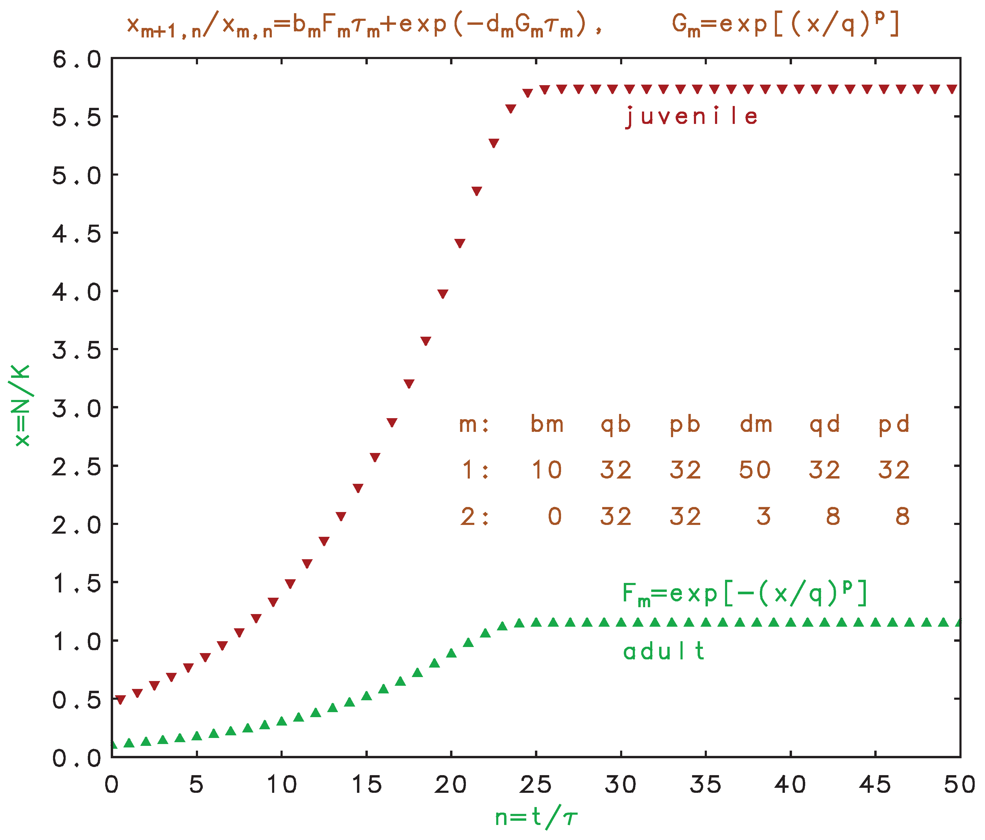
Equations can also represent discrete non-overlapping generations for metamorphic or spawning species if we let m count the life stages, such as larva, pupa, adult, and set for the breeding phase. Here, the prodigious output of many spawners is typically balanced by the low probability of survival of the pre-adult phases. This is consistent with the prior single-habitat, non-overlapping generations models, where the survival of the non-breeding phases is incorporated into the effective birth rate (sometimes denoted as the ”biotic potential”) in the adult phase. Splitting out the pre-adult phases, as done here, allows us to apportion the carrying capacities and mechanisms to the appropriate phases. In Figure 6, we show a hypothetical two-stage metamorphic species where the high death rate of the adults is sufficient to eliminate breeding survivors, but enough juveniles survive to allow overall growth until a saturation is reached near the non-breeder carrying capacity. We note that the differential model, Equation , with a higher death than birth rate, just leads to extinction, so is not valid for metamorphic species. The life stage problem has been addressed previously using matrix formulations (Leslie 1945, DeAngelis et al. 1980, Caswell 2006), but this is not necessary if all births transition to the next stage in the cycle, as shown here for metamorphic species.
6. Threshold Effects
Some species may require a critical density, , to survive or thrive, as discussed by Allee et al. (1949). This critical density could arise from the necessity to find a mate, establish a breeding colony, hunt cooperatively, school or flock, etc. Such threshold effects can be incorporated into the multi-habitat models above if the appropriate birth or death rates, or , are respectively multiplied or divided by another density-dependent factor, , that increases from a small residual value, , to 1 as x transitions through . should be chosen so that the death rate exceeds the birth rate, for example, for breeding thresholds or for survival thresholds. Some standard functions with this property are given by
Equation is a step function at , representing a sharp, definite threshold. This modification does not change the dynamics discussed above except when the populations dip below , whereupon they eventually go extinct. Equation represents a more gradual transition, characterized by the parameter. Equations are more probabilistic descriptions of this viability, representing a spread of effective critical densities given by a Lorentzian distribution, , or a Gaussian, , respectively. Because the modifying functions in Equations extend beyond the critical density, they may have a quantitative effect on the population dynamics, but the qualitative features discussed above remain. Such threshold effects may select against species whose population fluctuates wildly due to overbreeding (May and Oster 1976, Thomas et al. 1980).
7. Conclusions
We have shown, by the simple expediency of separating the density dependencies of the birth and death rates, that we can avoid the anomalous, unphysical behavior of the customary logistic model, Equations , for populations in excess of the carrying capacity. This procedure is essential for modeling the effects of sequential habitat variation encountered by seasonal breeders. The biological interpretation of the controlling density-dependent birth and death mechanisms is thereby more transparent, even in a single habitat. Simultaneously operative limiting mechanisms, including threshold effects, can be treated by multiplicative density-dependent functions. The disadvantages include numerical integration in place of analytical solutions and a great increase in the number of model parameters, some of which may be indeterminate in fitting population dynamics measurements. Some parameters can be specified independently by methods such as sampling, tagging and tracking. We have also demonstrated the deviations between continuous differential and discrete difference models, leading to time lags and possible inductive instabilities in the latter case.
These models may be useful to evaluate the factors limiting the abundance and distribution of migrating and resident seasonal species. In particular, they indicate how populations of migratory birds may be limited by non-breeding season habitat availability. More realistic behavior may require the inclusion of several other phenomena neglected here, such as immigration, stochastic processes and multi-species interactions. Application of the models for age-structured breeders may also be restricted, as shown for periodic breeders in an accompanying study (Pine and Rappole 2008).
References
- Allee, W.C.; Emerson, A.E.; Park, O.; Park, T.; Schmidt, K.P. Principles of animal ecology; Saunders: Philadelphia and London, 1949. [Google Scholar]
- Acheson, D. From calculus to chaos: an introduction to dynamics; Oxford University Press: Oxford, 1997. [Google Scholar]
- Beverton, R.J.H.; Holt, S.J. On the dynamics of exploited fish populations. Fishery Investigations, Series II 1957, 19, 1–533. [Google Scholar]
- Caswell, H. 2006. Matrix population models. Sinauer Assoc. Sunderland MA. DeAngelis, D.L., L.J. Svoboda, S.W. Christensen and D.S. Vaughan. 1980. Stability and return times of Leslie matrices with density-dependent survival: applications to fish populations. Ecological Modeling, 8:149-163.
- Fretwell, S.D. Populations in a seasonal environment; Princeton University Press: Princeton, 1972. [Google Scholar]
- Gilpin, M.E.; Ayala, F. J. Global models of growth and competition. Proceedings of the National Academy of Sciences (USA) 1973, 70, 3590–3593. [Google Scholar] [CrossRef] [PubMed]
- Kaitala, A.; Kaitala, V.; Lundberg, P. A theory of partial migration. American Naturalist 1993, 142, 59–81. [Google Scholar] [CrossRef]
- Kot, M. Elements of mathematical ecology; Cambridge University Press: Cambridge, 2001. [Google Scholar]
- Krebs, C.J. Ecology, the experimental analysis of distribution and abundance; Harper Collins College Publishers: New York, 1994. [Google Scholar]
- Kuno, E. Some strange properties of the logistic equation defined with r and K: Inherent defects or artifacts? Researches on Population Ecology 1991, 33, 33–39. [Google Scholar] [CrossRef]
- Leslie, P.H. The use of matrices in certain population mathematics. Biometrika 1945, 33, 183–212. [Google Scholar] [CrossRef] [PubMed]
- Leslie, P.H. Some further notes on the use of matrices in population mathematics. Biometrika 1948, 35, 213–245. [Google Scholar] [CrossRef]
- Lotka, A.J. Elements of mathematical biology; Dover Publications: New York, 1956. [Google Scholar]
- May, R. M. On relationships among various types of population models. American Naturalist 1973, 107, 46–57. [Google Scholar] [CrossRef]
- May, R.M. Simple mathematical models with very complicated dynamics. Nature 1976, 261, 459–467. [Google Scholar] [CrossRef] [PubMed]
- May, R.M.; Oster, G.F. Bifurcations and dynamic complexity in simple ecological models. American Naturalist 1976, 110, 573–599. [Google Scholar] [CrossRef]
- Maynard Smith, J. Mathematical ideas in biology; Cambridge University Press: Cambridge, 1968. [Google Scholar]
- Maynard Smith, J. Models in ecology; Cambridge University Press: Cambridge, 1974. [Google Scholar]
- Pearl, R. The growth of populations. Quarterly Review of Biology 1927, 2, 532–548. [Google Scholar] [CrossRef]
- Pearl, R.; Reed, L.J.; Kish, J.F. The logistic curve and the census count of 1940. Science 1940, 92, 486–488. [Google Scholar] [CrossRef] [PubMed]
- Pielou, E.C. An introduction to mathematical ecology; Wiley-Interscience: New York, 1969. [Google Scholar]
- Pine, A.S.; Rappole, J.H. Population limits with multiple habitats and mechanisms: II. age-structured periodic breeders. following paper. 2008. [Google Scholar]
- Press, W.H.; Teukolsky, S.A.; Vetterling, W.T.; Flannery, B.P. Numerical recipes in FORTRAN, 2nd ed.; Cambridge University Press: Cambridge, 1992. [Google Scholar]
- Rappole, J.H.; Morton, E.S.; Lovejoy, T.E., III; Ruos, J.S. Nearctic avian migrants in the neotropics; U.S. Dept. of Interior, Fish and Wildlife Service: Washington, 1983. [Google Scholar]
- Rappole, J.H. The ecology of migrant birds: a neotropical perspective; Smithsonian Institution Press: Washington, 1995. [Google Scholar]
- Richards, F.J. A flexible growth function for empirical use. Journal of Experimental Biology 1959, 10, 290–300. [Google Scholar] [CrossRef]
- Ricker, W.E. Stock and recruitment. Journal of Fisheries Research Board of Canada 1954, 11, 559–623. [Google Scholar] [CrossRef]
- Royama, T. Analytical population dynamics; Chapman & Hall: London, 1992. [Google Scholar]
- Sherry, T.W.; Holmes, R.T. Ch. 4 in Ecology and management of neotropical migratory birds; Martin, T.E., Finch, D.M., Eds.; Oxford University Press: Oxford, 1995. [Google Scholar]
- Skellam, J.G. Seasonal periodicity in theoretical population biology. Proceedings 5th Berkeley Symposium on Mathematical Statistics and Probability 1966, 4, 179–205. [Google Scholar]
- Sutherland, W.J. Predicting the consequences of habitat loss for migratory populations. Royal Society Proceedings 1996, B263, 1325–1327. [Google Scholar]
- Thomas, W.R.; Pomerantz, M.J.; Gilpin, M. E. Chaos, asymmetic growth and group selection for dynamic stability. Ecology 1980, 61, 1312–1320. [Google Scholar] [CrossRef]
- Verhulst, P.-F. Recherches mathématiques sur la loi d’accroissement de la population. Nouv. mém. de l’Academie Royale des Sci. et Belles-Lettres de Bruxelles 1845, 18, 1–41. [Google Scholar] [CrossRef]
- Verhulst, P.-F. Deuxième mémoire sur la loi d’accroissement de la population. Mém. de l’Academie Royale des Sci., des Lettres et des Beaux-Arts de Belgique 1847, 20, 1–32. [Google Scholar] [CrossRef]
- Weisstein, E.W. Logistic equation. mathworld.wolfram.com. 1999. Available online: http://mathworld.wolfram.com/LogisticEquation.html.
- Williamson, M. The analysis of biological populations; Edward Arnold Ltd.: London, 1972. [Google Scholar]
Figure 1.
(Color online) Upper panel: density dependence of birth and death rates for , with as noted, and . Lower panel: time development of population for single habitat for birth and death rates above, compared to Malthusian growth.
Figure 1.
(Color online) Upper panel: density dependence of birth and death rates for , with as noted, and . Lower panel: time development of population for single habitat for birth and death rates above, compared to Malthusian growth.
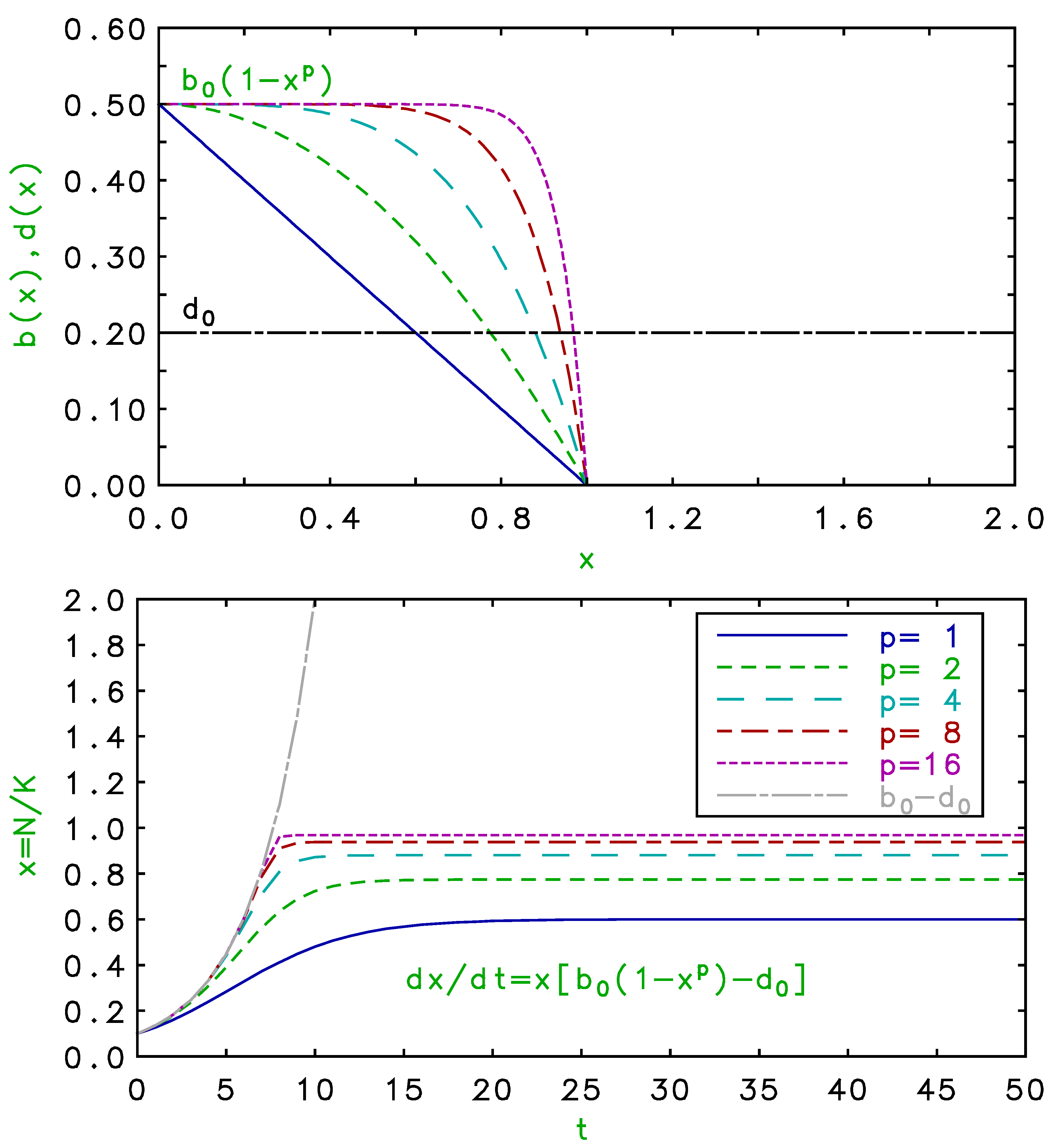
Figure 2.
(Color online) Upper panel: density dependence of birth and death rates for , , with and . Lower panel: time development of population for single habitat for birth and death rates above, compared to Malthusian growth.
Figure 2.
(Color online) Upper panel: density dependence of birth and death rates for , , with and . Lower panel: time development of population for single habitat for birth and death rates above, compared to Malthusian growth.
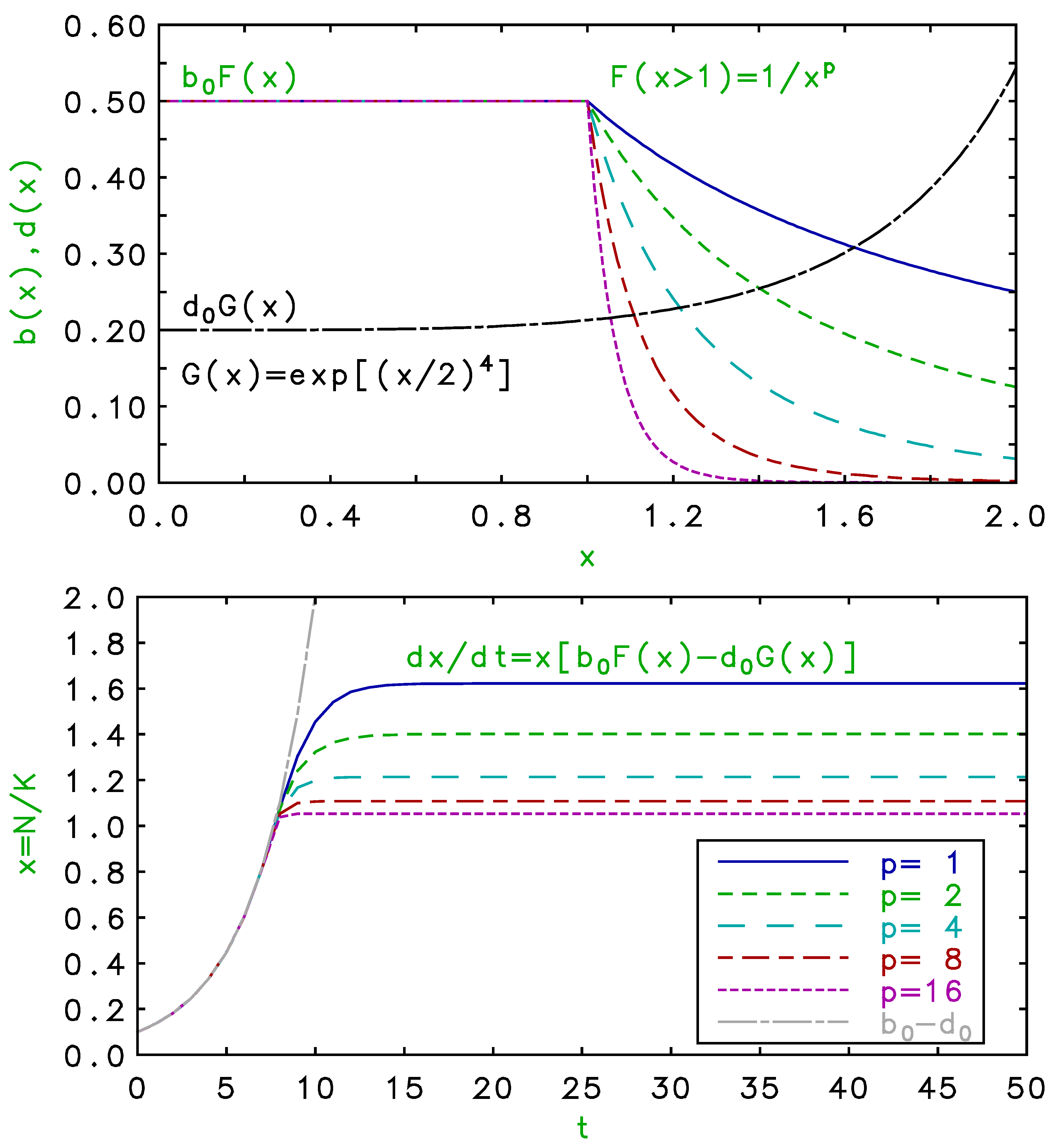
Figure 3.
(Color online) Time development of population for two sequential habitats for in first season only, with noted at right margin, and for both seasons of equal duration. Parameters tabulated on figure. Solid lines for continuous differential model and symbols for discrete difference model.
Figure 3.
(Color online) Time development of population for two sequential habitats for in first season only, with noted at right margin, and for both seasons of equal duration. Parameters tabulated on figure. Solid lines for continuous differential model and symbols for discrete difference model.
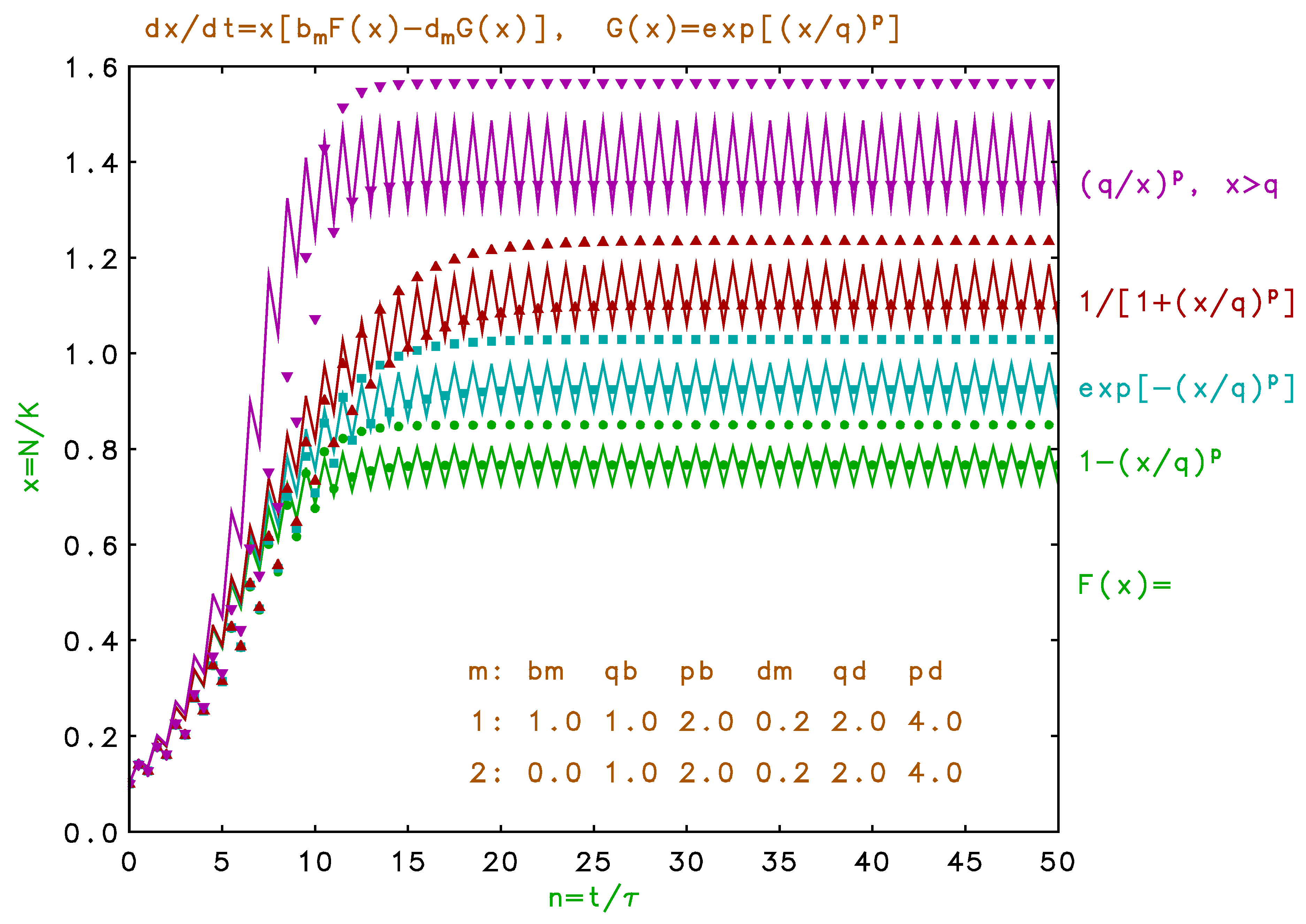
Figure 4.
(Color online) Time development of population for single habitat for , with noted at right margin, and . Parameters tabulated on figure. Solid lines for continuous differential model and symbols for discrete difference model.
Figure 4.
(Color online) Time development of population for single habitat for , with noted at right margin, and . Parameters tabulated on figure. Solid lines for continuous differential model and symbols for discrete difference model.
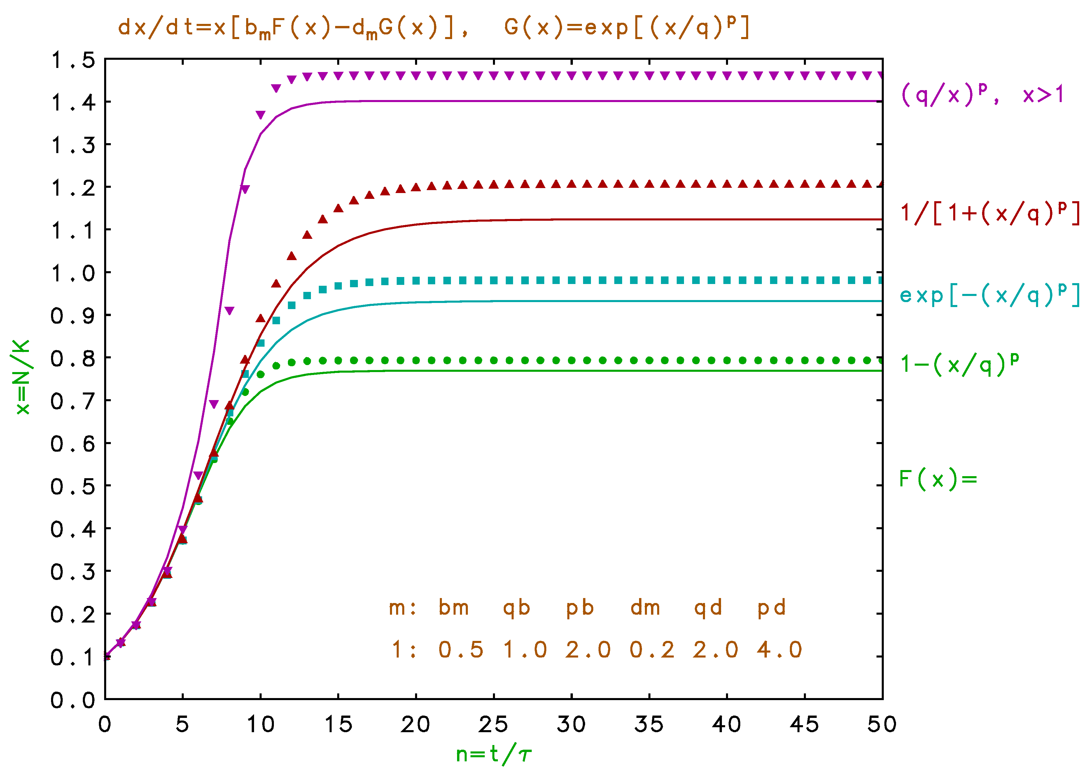
Figure 5.
(Color online) Same as Figure 4 with birth rate four times higher, indicating instabilities from discrete model delays.
Figure 5.
(Color online) Same as Figure 4 with birth rate four times higher, indicating instabilities from discrete model delays.
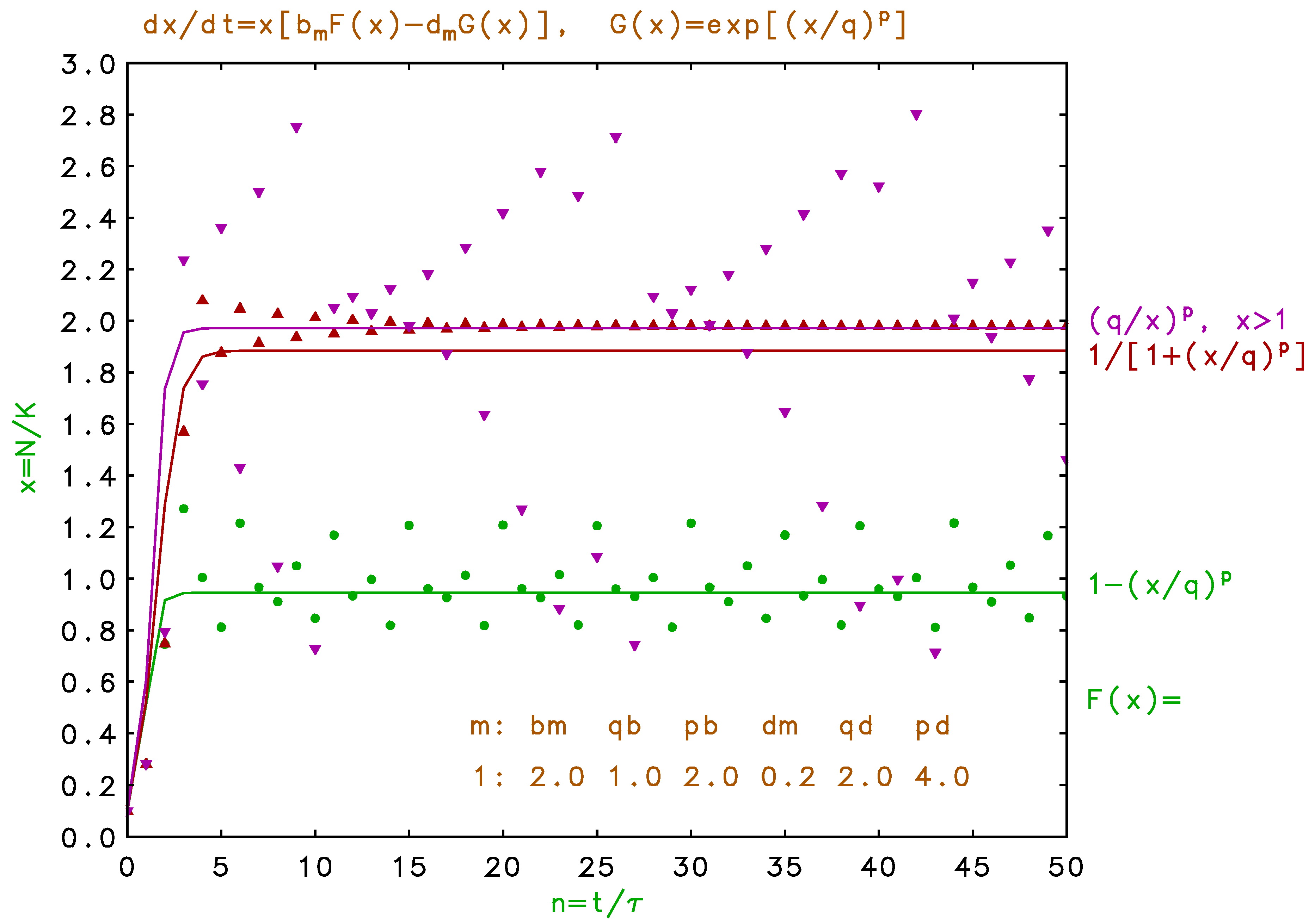
Figure 6.
(Color online) Discrete model time development of metamorphic species with two stages of equal duration. Only adults breed and then die off; enough juveniles survive to eventually approach their carrying capacity.
Figure 6.
(Color online) Discrete model time development of metamorphic species with two stages of equal duration. Only adults breed and then die off; enough juveniles survive to eventually approach their carrying capacity.
Disclaimer/Publisher’s Note: The statements, opinions and data contained in all publications are solely those of the individual author(s) and contributor(s) and not of MDPI and/or the editor(s). MDPI and/or the editor(s) disclaim responsibility for any injury to people or property resulting from any ideas, methods, instructions or products referred to in the content. |
© 2026 by the authors. Licensee MDPI, Basel, Switzerland. This article is an open access article distributed under the terms and conditions of the Creative Commons Attribution (CC BY) license (http://creativecommons.org/licenses/by/4.0/).
Copyright: This open access article is published under a Creative Commons CC BY 4.0 license, which permit the free download, distribution, and reuse, provided that the author and preprint are cited in any reuse.


