Microfluidic Interrogation of Chitin-Induced Calcium Oscillations in the Moss Physcomitrium patens

1. Introduction

The ability of plants to sense and respond to biotic stressors, such as fungal, bacterial, and viral pathogens, is crucial for survival. Mosses share innate immune systems with vascular plants and evolved defense mechanisms that further enable pathogen resistance. For example, during the attack of a fungal predator, moss plants can detect a pathogen-associated molecular pattern (PAMP) at surface-localized pattern-recognition receptors (PRRs) and initiate a PAMP-triggered immune response. Once activated, cells exhibit a simultaneous rapid influx of cytosolic calcium (Ca²⁺) and activation of the mitogen-activated protein kinase (MAPK) phosphorylation cascade. The resulting defense response propagates plant-wide and includes production of reactive oxygen species (ROS), defense gene activation, and hormone synthesis leading to programmed cell death, growth inhibition, and cell wall reinforcement [1,2,3,4]. Many processes modulate pathogen resistance including circadian rhythms; for example, Arabidopsis susceptibility to B. cineria fungus is decreased at dawn when biotrophic predators primarily release spores [5].

Calcium signaling plays a vital role in these responses. Stimulation with chitin oligosaccharides, a component of the fungal cell wall, caused plant-wide cytoplasmic Ca²⁺ oscillations and induction of defense gene expression [3]. Calcium influx alone by ionomycin treatment was sufficient to induce the acute phase of defense gene expression, suggesting a direct role in the process, but not the sustained, elevated level following chitin exposure. The details by which calcium levels and oscillation frequency affect gene expression and other pathogen responses, and how calcium and other signals propagate within and between cells, remain largely undetermined [6].

This study addresses these questions using new experimental methods for the measurement and analysis of pathogen-triggered Ca²⁺ responses at plant-wide, single-cell, and subcellular levels. The moss P. patens is an advantageous model for studying plant-pathogen interactions due to its conserved defense mechanisms, genomic toolset, rapid growth, and small size [7]. In particular, the juvenile protonemal stage of P. patens has a filamentous morphology composed of linear and branching chains of chloronemal (CH) and caulonemal (CA) cells. Chloronemata contain an abundance of chloroplasts for photosynthetic energy production. Caulonemata are longer, thinner, and faster growing than chloronemata [8,9], attributes that are key for building plant mass and for nutrient acquisition. These cell types exhibit different calcium responses related to their position within the filament and growth status. For example, the apical regions of growing caulonema tip cells exhibit Ca²⁺ oscillations that promote the dissipation of actin filaments as required for growth [3,10]. Prior studies utilizing protonemata have focused primarily on these growing tip cells, or on average calcium levels across the entire plant which obscures cell-type variation and signal propagation [6].

To explore individual cell responses across entire plants, we used wide-field fluorescent imaging of plants expressing a genetically-encoded calcium indicator [11,12,13]. Recently, microfluidic devices were fabricated to grow and image plants while keeping them physically within a narrow imaging focal plane [9,14,15]. In addition, microfluidics enables the study of biological phenomena in precise chemical and mechanical microenvironments [16,17,18]. Specifically, laminar fluid flow permits precise and predictable spatiotemporal stimulus patterns, including the ability to rapidly introduce and remove chemicals [19]. Here, we present microfluidic devices capable of dynamically stimulating multiple plants at once during time-lapse calcium imaging. Similar to prior devices, we demonstrated that protonemata housed in microfluidics triggered intracellular calcium waves comparable to studies that stimulated plants on coverslips. Further, we show for the first time how calcium dynamics react to stimulus removal and to repeated stimulation for different durations. We additionally examined the effects of adaptation time within the microfluidic environment, timing of stimulation relative to circadian cycles, and variations among cell types.

In functional imaging studies, data analysis can be a substantial bottleneck. Each timelapse image stack may require manual annotation and corrections to address sample movement or illumination artifacts. To increase experimental throughput, reduce bias, and increase reproducibility, we developed and validated a semi-automatic, unbiased clustering algorithm to locate contiguous regions within the plants exhibiting distinct calcium dynamics. These regions included whole individual cells as well as subcellular regions. We report the spontaneous and chitin-elicited responses across cell types and subcellular regions to long and short chitin exposures, and highlight differences in response due to time of day, adaptation in the device. Together, these microscopy, microfluidic, and data analysis methods enable the broad study of plant responses to dynamic, reversible stimuli and underlying calcium signaling.

2. Results

2.1. Microfluidic Stimulation and Calcium Recording

Plants expressing the cytoplasmic calcium indicator GCaMP6f [3,20] were imaged in a microfluidic flow chamber to visualize spontaneous and chitin-induced responses from multiple plants at once (Figure 1a, b). Plants between 6-8 days old were loaded into the fluid-filled microfluidic channels by syringe (Figure 1b, c) and allowed to adapt to the microfluidic environment for up to 3 h in darkness with continuous flow of plant medium. Calcium levels were recorded at 1 fps by epifluorescence microscopy. The application and removal of stimulus solutions was automated and reversible, switching completely within 2 seconds and remaining stable for minutes to hours (Figure 1c, d).

2.2. Identification of Plant Regions and Calcium Waves

Image stacks were cropped and segmented to automatically identify regions of interest (ROIs), as described in detail in Methods Section 4.8 (Figure 1e). Briefly, k-means clustering grouped individual image pixels by similarity of their fluorescence intensity dynamics, treating each time point as a separate dimension, followed by editing for ROI connectivity and size limits (see Figure 6, below). To assess automatic segmentation quality, plant cell borders were stained after calcium recordings using Direct Yellow 96 and manually segmented (Figure 1f). Typical cells were represented by one to three ROIs, reflecting distinct sub-cellular calcium dynamics.

Observation of tip cells revealed three common calcium oscillation patterns (Figure 1g, Supplementary Video 1). First, the apical tip region initiated a calcium wave, followed by directional propagation to subapical cells over about 1 min. Second, the tip initiation subsided without any propagation to adjacent sub-cellular regions or cells. Third, synchronous activation of cells and regions arose and subsided without directional propagation (Figure 1h). Because directional propagation occurred within plant cells, averaging fluorescent intensity within cell regions could obscure these dynamics (Figure 1i). Therefore, we used the automatically segmented ROIs to investigate plant-wide responses to different chitin stimulation patterns and other experimental conditions.

2.3. Chitin Elicits Distinct Calcium Oscillations Across Plants

In the first experiment set, plants were allowed 3 hr to adapt to the microfluidic arena in darkness after entering the device. Each experiment included a 30 min period exposing plants to plant media, followed by a 30 min period of chitin exposure (Figure 2). A small, representative 11-cell plant is shown in Figure 2a, divided into 14 ROIs with distinct calcium dynamics (Figure 2b, c). Calcium fluorescence remained low during the 30 min buffer flow, followed by a rapid rise upon chitin addition that subsided over 3 to 7 min (see Supplementary Video 2). During the initial response period some cells exhibited a burst of peaks before they transition to regular, repeating calcium waves (Figure 2d). The initial response latency between chitin addition and calcium rise varied from 16 to 32 s across the plant (22.6 ± 4.5 s, mean ± SD to 10% peak level, Figure 2e). The instantaneous probability of calcium waves across all 14 ROIs was low during buffer (5.2 ± 4.7%), reached 100% within 1 min of stimulus onset (Figure 2f), and settled to an average of 44% at any moment during chitin stimulation.

To quantify wave parameters, we identified each calcium wave and analyzed its magnitude and timing, including rise time, fall time, duration, and interval. Calcium fluorescence intensity varies across ROIs (see Methods and Figure 6). However, when normalized to the peak initial chitin response, calcium wave dynamics appeared similar both within and across ROIs (Figure 2d). Calcium oscillations occurred at different intervals, ranging from 1.1 – 4.6 min (63 – 276 s, Figure 2g, h). Within each ROI, interval variance was lower (CV 19.2 ± 11.1%) than across all ROIs (CV 45.4%), indicating that each cell had a characteristic frequency response (Figure 2h). Because the wave interval varied across the plants, adjacent cells did not oscillate in synchrony, as might be anticipated from the diffusion of calcium across plasmodesmata. Instead, only ROIs within the same cell showed high maximal response cross-correlation, a measure of synchrony independent of fixed phase shifts (Figure 2i). Notably, the site of wave initiation and direction of propagation were not static throughout stimulation, even within a single cell.

We next asked whether individual Ca²⁺ wave dynamics (for example, rise and fall times) were stereotyped or scaled with overall oscillation frequency. Calcium wave duration ranged from 30 – 110 s and was only slightly correlated with wave interval (R = +0.14) and its inverse, wave frequency (R = –0.16) (Figure 2j). In contrast, rise and fall times correlated strongly and equally with wave duration (R = 0.79–0.84), reflecting a symmetric, Gaussian wave shape (Figure 2k). Together, these results suggest that calcium waves are initiated in different cells at different intervals, but individual wave dynamics are similar and preserve the bell curve shape as calcium levels rise and fall.

These results were representative across nine plants divided into 213 ROIs. Before chitin addition, spontaneous calcium waves were variable and rare (1.3 ± 3.2 per 30 mins), increasing dramatically and consistently across ROIs during chitin exposure (9.6 ± 3.1 waves per 30 min). Chitin-induced oscillations were four times stronger (ΔF/F₀ = 2.7 vs. 0.7, p<0.0001) than spontaneous Ca²⁺ oscillations and occurred four times more often (Figure 2l). Calcium waves in chitin occurred at an average frequency of 0.8 ± 0.5 min^-1 (interval 159.7 ± 64.5 s, interquartile range 127.5 to 181.0 s) in the microfluidic setup, comparable to prior observations [3]. Individual plants responded similarly, with plant-wide mean chitin-induced wave intervals ranging from 142 to 218 s (Supplementary Figure 1). Chitin-induced waves were ~20% longer in duration (72 s vs. 61 s), exhibited slightly longer rise times (27 s vs. 25 s), and coincided with higher baseline calcium levels preceding and following each oscillation compared to spontaneous waves.

Figure 2. Chitin elicits persistent plant-wide calcium oscillations. (a) Example moss plant in brightfield imaging with cell borders delineated in yellow. (b) Fluorescent image of GCaMP indicating intracellular calcium levels, taken from one frame of a 60-minute timelapse. (c) Automatically segmented ROIs (see Figure 6 for method depiction). Scale bars (a-c), 25 µm. (d) Calcium fluorescence integrated across each ROI, normalized to the peak response at chitin stimulus onset. Plants in the microfluidic device were allowed to adapt for 3 hrs, then imaged for 60 min with 30 min of buffer and 30 min of 2.2 mg/mL chitin stimulus. (e) Expanded timescale of calcium response in (d), showing response latency (stimulus onset to 10% peak intensity). (f) The probability of calcium waves rose at chitin onset, followed by oscillating probability during continuous 30 min stimulation. (g) Heatmap of normalized calcium fluorescence from (d). (h) Intervals between calcium waves varied across ROIs. (i) Maximum cross-correlation heatmap shows little temporal correlation among ROIs, except for ROIs within the same cell (1-2, 3-4, 10-11). (j) Individual normalized calcium waves (n = 133) show symmetric onset and offset within a tight range of FW10 duration. Quartile averages are plotted below. (k) Calcium wave duration was strongly and positively correlated with wave rise and fall times (10% to 90%) but only weakly correlated with wave interval and frequency. (l) Comparison of calcium dynamics before (gray) and after (purple) chitin stimulation for nine plants. Chitin increased the number of waves per 30 mins, the peak calcium fluorescence, the wave frequency, and the baseline calcium signal (relative to wave peak height). Chitin increased the duration of each calcium wave (full-width, 10% maximum, FW10) and, to a lesser extent, the rise time (10% to 90%). (m) ROIs were mapped to six moss ROI types and regions as indicated for the plant in (a-e) and seven additional plants. Caulonema tip cells were divided into the apex tip region (CA*) and the remainder of the cell (CA). Both CA and chloronema (CH) tip cells were distinguished from adjacent subapical cells (CAs and CHs) and branch (B) cells budding from central branch points. (n) Across eight plants, chitin stimulation elicited faster calcium waves in all ROI types except CA*, whose interval increased. Values were log-transformed before one-way ANOVA. Bars represent median, interquartile range, and individual wave data points (number listed at the base of each bar). (o) Calcium wave durations were dependent on cell type and region, plotted as in (g). Differences between groups were analyzed via one-way ANOVA. **, p<0.0001; *, p<0.001; +, p<0.01; ns, not significant.

Figure 2. Chitin elicits persistent plant-wide calcium oscillations. (a) Example moss plant in brightfield imaging with cell borders delineated in yellow. (b) Fluorescent image of GCaMP indicating intracellular calcium levels, taken from one frame of a 60-minute timelapse. (c) Automatically segmented ROIs (see Figure 6 for method depiction). Scale bars (a-c), 25 µm. (d) Calcium fluorescence integrated across each ROI, normalized to the peak response at chitin stimulus onset. Plants in the microfluidic device were allowed to adapt for 3 hrs, then imaged for 60 min with 30 min of buffer and 30 min of 2.2 mg/mL chitin stimulus. (e) Expanded timescale of calcium response in (d), showing response latency (stimulus onset to 10% peak intensity). (f) The probability of calcium waves rose at chitin onset, followed by oscillating probability during continuous 30 min stimulation. (g) Heatmap of normalized calcium fluorescence from (d). (h) Intervals between calcium waves varied across ROIs. (i) Maximum cross-correlation heatmap shows little temporal correlation among ROIs, except for ROIs within the same cell (1-2, 3-4, 10-11). (j) Individual normalized calcium waves (n = 133) show symmetric onset and offset within a tight range of FW10 duration. Quartile averages are plotted below. (k) Calcium wave duration was strongly and positively correlated with wave rise and fall times (10% to 90%) but only weakly correlated with wave interval and frequency. (l) Comparison of calcium dynamics before (gray) and after (purple) chitin stimulation for nine plants. Chitin increased the number of waves per 30 mins, the peak calcium fluorescence, the wave frequency, and the baseline calcium signal (relative to wave peak height). Chitin increased the duration of each calcium wave (full-width, 10% maximum, FW10) and, to a lesser extent, the rise time (10% to 90%). (m) ROIs were mapped to six moss ROI types and regions as indicated for the plant in (a-e) and seven additional plants. Caulonema tip cells were divided into the apex tip region (CA*) and the remainder of the cell (CA). Both CA and chloronema (CH) tip cells were distinguished from adjacent subapical cells (CAs and CHs) and branch (B) cells budding from central branch points. (n) Across eight plants, chitin stimulation elicited faster calcium waves in all ROI types except CA*, whose interval increased. Values were log-transformed before one-way ANOVA. Bars represent median, interquartile range, and individual wave data points (number listed at the base of each bar). (o) Calcium wave durations were dependent on cell type and region, plotted as in (g). Differences between groups were analyzed via one-way ANOVA. **, p<0.0001; *, p<0.001; +, p<0.01; ns, not significant.

2.4. Calcium Wave Dynamics Differ Among Cell Types and Subcellular Domains

We next assessed whether different cell types exhibited distinct calcium dynamics, propagation rates, or directionality within the protonemal filaments. Chloronemal cells regenerate from the protoplast for the first 6 to 7 days, until spatial cues and auxin signaling enable differentiation of the apical cells into caulonemata [9]. The growing apical caulonemal cells exhibit a tipward Ca²⁺ gradient characterized by rapid oscillations (<1 min interval), similar to other tip-growing plants, and the application of chitin oligosaccharides rapidly inhibits growth and dissipates the tip-localized gradient within 1 – 2 min of perception [1,3,10].

The automatic segmentation algorithm extracted 1 to 3 ROIs per cell, whose borders were delineated manually using high-resolution Z-stack images acquired after timelapse acquisition. Caulonemal (CA) tip cells were often separated into multiple ROIs, capturing the distinct dynamics exhibited near the apical tip (CA*) prior to chitin application. Spontaneous calcium waves were rare in most cell types except the CA* apical tip region, which exhibited waves with an median interval of 85.5 s (59.0 – 235.8 interquartile range), consistent with prior reports of moss cultured on cover slips. Chitin addition induced similar calcium waves within the whole plant, oscillating at a mean interval of 156.4 ± 6.7 s across all cell types (Figure 2n). The fast spontaneous calcium waves in the CA* apical tip regions slowed 39% by chitin exposure, but still oscillated slightly quicker (144.6 s) than both chloronemal subapical cells (CHs) and tip (CH) cells (167.7 s and 161.8 s, respectively, p<0.05). Additionally, chitin increased wave duration in both CA* apical tip regions (+26%, p<0.0001) and CH cells (+19%, p<0.001). No other cell types featured a significant change in wave durations when compared to their baseline values (Figure 2o). Interestingly, during chitin stimulation, subapical cells exhibited ~5 s shorter duration waves than tip cells for both chloronemal (CHs 72.4 s vs. CH 79.1 s) and caulonemal (CAs 66.2 s vs. CA 71.4 s, CA* 70.1 s), while branching cell wave durations were similar to their neighboring subapical cell (B 71.8 s).

Figure 3. Calcium waves are modulated by adaptation time and by circadian rhythms. (a) Normalized heatmaps of plant ROIs during 30 min buffer flow and 30 min chitin stimulation. Plants were adapted in the microfluidic device for 3 h or 30 min, and images were taken during daytime (dawn-to-dusk) or nighttime, as indicated by the sun and moon icons. Calcium fluorescence is normalized to the minimum and peak intensity per ROI. Data represent n = 149 – 495 ROIs from 3–9 plants. (b) Mean ROI responses are shown as normalized fluorescence intensity averaged across all ROIs per condition (black line) or as the probability of a calcium wave over time (shading). Bars and shading represent the chitin stimulation time (from 30 – 60 min). (c-g) Comparison of calcium wave dynamics before and after chitin addition across adaptation and day/night conditions. Data represent (c) the number of waves per 30 min period (buffer or stimulus); (d) Peak calcium wave fluorescence, dF/F₀; (e) calcium wave frequency per minute; (f) calcium wave duration (above 10% of maximum prominence, i.e. FW10); and (g) relative calcium fluorescence baseline at the beginning of each wave. **, p<0.0001; *, p<0.001 for buffer vs. stimulus or specified comparison; +, p<0.0001 compared with buffer, 3h adaptation, daytime condition. Data represent mean and SD, n = 91 – 4592 waves. (h) The response delay (sec) between stimulus application and initial response onset (above 10% of maximum prominence). **, p<0.0001; *, p<0.001 compared between both time of day and adaptation time duration. Data represent n = 149 – 407 waves.

Figure 3. Calcium waves are modulated by adaptation time and by circadian rhythms. (a) Normalized heatmaps of plant ROIs during 30 min buffer flow and 30 min chitin stimulation. Plants were adapted in the microfluidic device for 3 h or 30 min, and images were taken during daytime (dawn-to-dusk) or nighttime, as indicated by the sun and moon icons. Calcium fluorescence is normalized to the minimum and peak intensity per ROI. Data represent n = 149 – 495 ROIs from 3–9 plants. (b) Mean ROI responses are shown as normalized fluorescence intensity averaged across all ROIs per condition (black line) or as the probability of a calcium wave over time (shading). Bars and shading represent the chitin stimulation time (from 30 – 60 min). (c-g) Comparison of calcium wave dynamics before and after chitin addition across adaptation and day/night conditions. Data represent (c) the number of waves per 30 min period (buffer or stimulus); (d) Peak calcium wave fluorescence, dF/F₀; (e) calcium wave frequency per minute; (f) calcium wave duration (above 10% of maximum prominence, i.e. FW10); and (g) relative calcium fluorescence baseline at the beginning of each wave. **, p<0.0001; *, p<0.001 for buffer vs. stimulus or specified comparison; +, p<0.0001 compared with buffer, 3h adaptation, daytime condition. Data represent mean and SD, n = 91 – 4592 waves. (h) The response delay (sec) between stimulus application and initial response onset (above 10% of maximum prominence). **, p<0.0001; *, p<0.001 compared between both time of day and adaptation time duration. Data represent n = 149 – 407 waves.

2.5. Device Adaptation Time

Plants introduced into the microfluidic arenas experienced a different local environment compared to cultivation, and some mechanical perturbation during loading into the microfluidic device. For example, moss plants were collected into a loading syringe and gently injected into the device through a loading port. We therefore tested how adaptation time in the device influenced the chitin-induced calcium responses (Figure 3a, b). Plants allowed to acclimate to darkness and the microfluidic environment for only 30 min before imaging showed several prominent spontaneous calcium waves (3.1 ± 2.6 per 30 min) before the addition of chitin, unlike plants acclimated for 3 h (0.2 ± 0.6 per 30 mins, Figure 3c). After stimulation, no difference was noted in the number, frequency, or duration of calcium oscillations, although peak and baseline GCaMP fluorescence levels were reduced with short 30 min adaptation (Figure 3c-g). Thus, the extended 3 hr adpatation time appeared to quiet spontaneous calcium waves and magnify chitin-triggered responses, with no change in stimulated wave dynamics.

2.6. Circadian Modulation of Ca²⁺ Waves

Plants modulate core processes such as defense and growth according to the time of day, due to their reliance on light for energy and its diurnal variation [21]. Moss protonemal cells exhibit a Circadian Clock-Associated 1 (CCA1) homolog whose expression becomes maximized near dawn [22]. We therefore investigated whether chitin-induced calcium wave dynamics were modulated by stimulation time relative to the day/night circadian cycle.

Whereas long-adapted plants stimulated during daytime rarely showed spontaneous calcium waves, stimulation during nighttime elicited strong spontaneous waves (Figure 3a). Remarkably, a strong calcium wave appeared consistently in nighttime stimulated plants within minutes of timelapse acquisition (89% of ROIs active at 85 sec, Figure 3b), coinciding with the first exposure of blue fluorescence excitation light. Following about 10 min of quiescence, about 90% of ROIs displayed additional spontaneous Ca²⁺ waves for the remainder of the baseline period. During this time, Ca²⁺ waves traveled slowly within and between the cells of these plants (Supplementary Video 3).

After chitin stimulation, long-adapted plants exhibited nearly twice as many calcium waves in daytime (7.5 ± 3.2 waves) than in nighttime (3.5 ± 2.4 waves, p<0.001), while no difference was seen for the short-adapted group (7.2 ± 3.0 vs. 7.2 ± 2.1 waves, Figure 3c). The peak fluorescence values increased significantly during stimulation for all experimental groups (Figure 3d, excluding the first wave of the long-adapted nighttime plants which may represent a blue-light sensitivity artifact). Spontaneous wave frequency was lower in nighttime long-adapted plants than daytime, but equal in short-adapted plants, and wave frequency increased in all conditions compared with spontaneous waves (Figure 3e). Faster oscillations were similar across plants, regions, and cell types (Supplementary Figure 2). Calcium waves were ~10s longer during stimulation, and ~20s longer at night than during the day in long-adapted plants, but similar for all conditions in short-adapted plants (Figure 3f). Baseline calcium levels during stimulation were also modulated by time of day (lower at night) only in long-adapted plants (Figure 3g).

In spontaneously-active regions of long-adapted plants at night, the initial chitin-induced response was delayed three-fold (55 ± 32 s) compared with the daytime plants (16 ± 14 s, p<0.001), suggesting that recent calcium activity slowed subsequent stimulus-evoked responses in long-adapted plants (Figure 3h). In short-adapted plants, the response delays were more similar but still longer at night (37 ± 34 s night vs. 29 ± 24 s day, p<0.01). The initial chitin-onset response was more synchronized in daytime-stimulated plants (especially after long adaptation, 14 s SD) and more variable in nighttime (32 – 34s SD).

Taken together, the long 3h adaptation time in the microfluidic environment decreased baseline calcium levels and spontanous oscillations, but did not affect chitin-stimulated activity. Circadian rhythms affected spontaneous activity and stimulated wave frequency after long adaptation, but had little effect in short-adapted plants, suggesting that the experimental microenvironment plays a stronger role in calcium dynamics.

2.7. Calcium Waves Elicited by Repeated Stimuli

A key benefit of microfluidic stimulation is the ability to deliver repeated pulses separated by complete wash out of the stimulus solution. To analyze the repeatability of chitin-elicited calcium signals, we applied five consecutive 5-min stimulus pulses, with 5 min of buffer flow between each stimulation. A similar duration exposure to chitin oligosaccharides was sufficient to upregulate defense gene expression [3,9].

Calcium waves were initiated by each individual chitin application and ceased after each chitin removal, with dynamics that were modulated by adaptation time and by time of day (Figure 4a, b). The long-adapted plants featured little calcium activity in plant medium between pulses, similar to the quiet pre-stimulation period in Figure 3. In the daytime, the first pulse produced a sustained calcium response, as during the first few minutes of the 30-min stimulation. In contrast, later pulses produced calcium waves that were highly synchronized, with nearly all ROIs initiating calcium waves about 1 min after stimulation (Figure 4b). Responses adapted to repeated chitin pulses, with integrated fluorescence (AUC, area under curve) decreasing steadily over time (Figure 4c). Relatedly, the 5-min chitin pulses produced either one or two synchronized calcium waves, with the number of doubled waves decreasing for later repeats (Figure 4d).

Calcium waves also became more delayed and less synchronized for each chitin pulse. Response delay, or the mean time between stimulus application and response initiation, increased three-fold from 25 s to 64 s (Figure 4e). Response synchrony decreased over time, as the standard deviation of the response delays increased from 10 to 16 s (Figure 4e). Wave duration also decreased over repeated pulses, except the first pulse wave appeared shorter as calcium levels remained above baseline (Figure 4f).

At nighttime, the long-adapted plants showed similar trends in response adaptation to daytime. Each 5-min chitin pulse elicited one and occasionally two calcium waves, but less frequently than during daytime, as wave intervals were slightly longer at night (Figure 4d). Nighttime waves had 20 – 30% longer response delays than daytime, increasing from 33 s to 76 s from first to fifth pulse, and less response synchrony (i.e., 30 to 60% increased delay SD), rising from 13 s to 26 s from pulse 1 to 5) (Figure 4e). Wave durations were more consistent across repeats at night (Figure 4f).

Short-adapted plants had more spontaneous calcium waves outside of chitin stimulation (about 1 per 5-min) and more chitin-evoked waves (about 2 per 5-min cycle) than long-adapted plants (Figure 4a ,d). While the number of waves per pulse remained steady across repeats, response adaptation manifested as a steady decline in integrated response (AUC) over time (Figure 4c). Response delays were elevated with short adaptation time, with a mean delay increasing from 35 to 87 s over the 5 repeats during the day, and from 45 to 90 s at night (Figure 4e). Response synchrony was substantially lower in short-adapted plants. Again, time of day played little role in short-adapted plants, with similar calcium wave number, magnitude, onset delay, or duration in day and night experiments.

2.8. Plant-Wide Calcium Oscillations Are Driven by Short-Pulse Stimulation Frequency

Since five-minute duration pulses elicited an initial calcium wave, followed occasionally by a second wave, we reasoned that shorter chitin stimulation should elicit a single, synchronized calcium wave for each brief chitin pulse. Indeed, 1 minute of chitin exposure was sufficient to elicit a calcium wave in nearly every ROI (Figure 5a-c). Over 88% of all ROIs responded to all ten repeated 1-min pulses, and 95% of them initiated calcium waves to the first seven pulses (Figure 5c). Calcium oscillations were effectively driven at chitin stimulation frequency, with a median interval of 244 s (4.07 min), or just 2% above the 4-min chitin pulse interval, and consistent across the ten repeats (Figure 5d). Calcium waves were initiated 47.5 ± 24 s (SD) after chitin addition, with a gradual increase in response latency from the first pulse (39.0 ± 14.8 s) to the last four pulses (56.1 ± 25.7 s) (Figure 5e).

Wave durations averaged 82.1 ± 15.0 s and were consistent for all ten pulses (Figure 5f) and similar to durations for 30 min stimulations (Figure 3f). Chitin removal did not suppress or shorten calcium wave activity; in fact, nearly all (99.8%) waves concluded at least 20 s after chitin was removed (mean 67.8 ± 24.1 s). About 26% of waves were initiated after chitin removal (Supplementary Figure 3). This suggests that the process of wave initiation begins before calcium rises to detectable levels and is not terminated once stimulation ceases.

3. Discussion

This study expands upon prior investigations of calcium oscillations in P. patens moss protonemal cells, combining epifluorescent calcium imaging of plants expressing the GCaMP indicator with microfluidic devices for rapid and reversible chemical stimulation. We demonstrated tip-localized calcium oscillations indicative of tip-growth and plant-wide calcium oscillations upon introduction of chitin oligosaccharides, and measured calcium dynamics that resembled prior studies on agar and in microfluidic growth chambers [1,3]. We further illustrate, for the first time: (1) calcium response variations among different cell types and subcellular regions; (2) response modulation by adaptation time and by experimental time of day relative to circadian rhythms; (3) responses to the sudden removal of chitin stimulus; (4) responses to repeated pulses and response adaptation over repeated stimulation; and (5) the ability to drive plant-wide calcium oscillations at a prescribed frequency. We characterized calcium wave dynamics for each experimental condition across several parameters, including rates, durations, intervals, probabilities, and variabilities, as a baseline for comparison and to inform future experimental designs. We validated an unbiased, pixel-based k-means clustering approach to automatically extract ROIs exhibiting calcium wave dynamics which differ in time of initiation, direction of propagation, or oscillation frequency, and developed data analysis software to extract, summarize, and combine results from multiple individual plants.

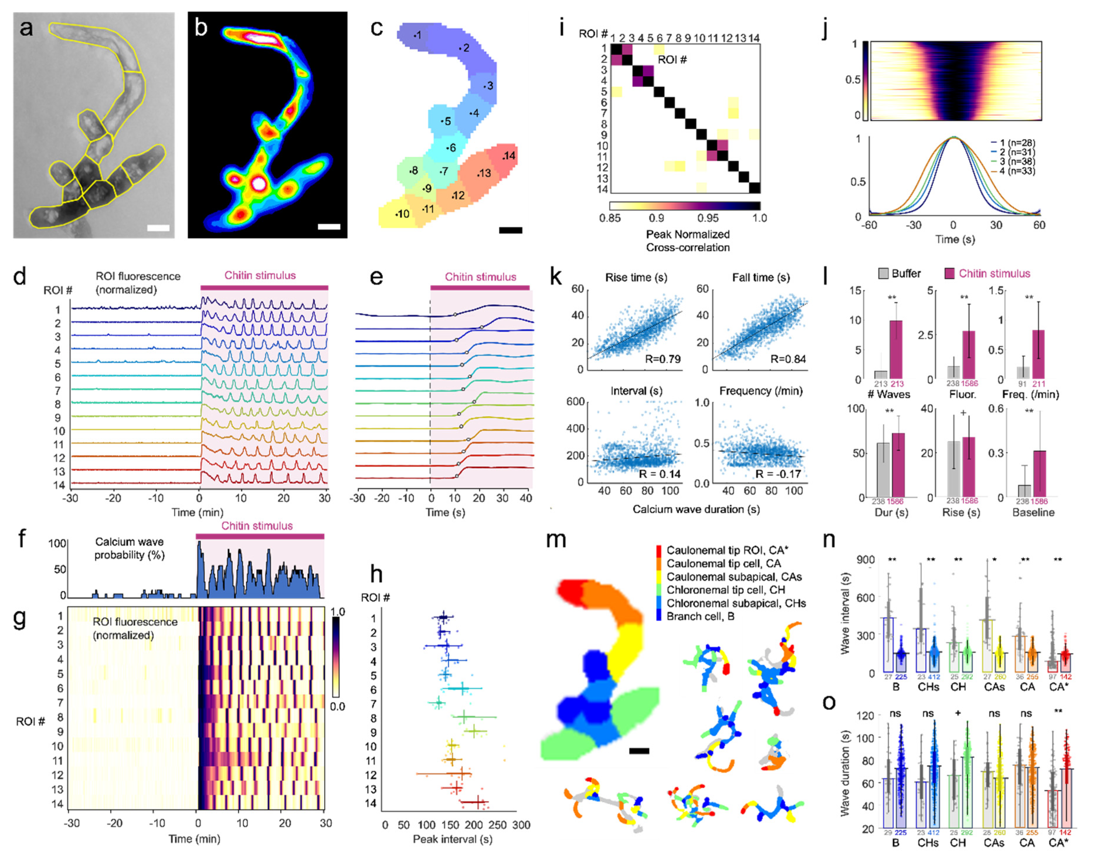
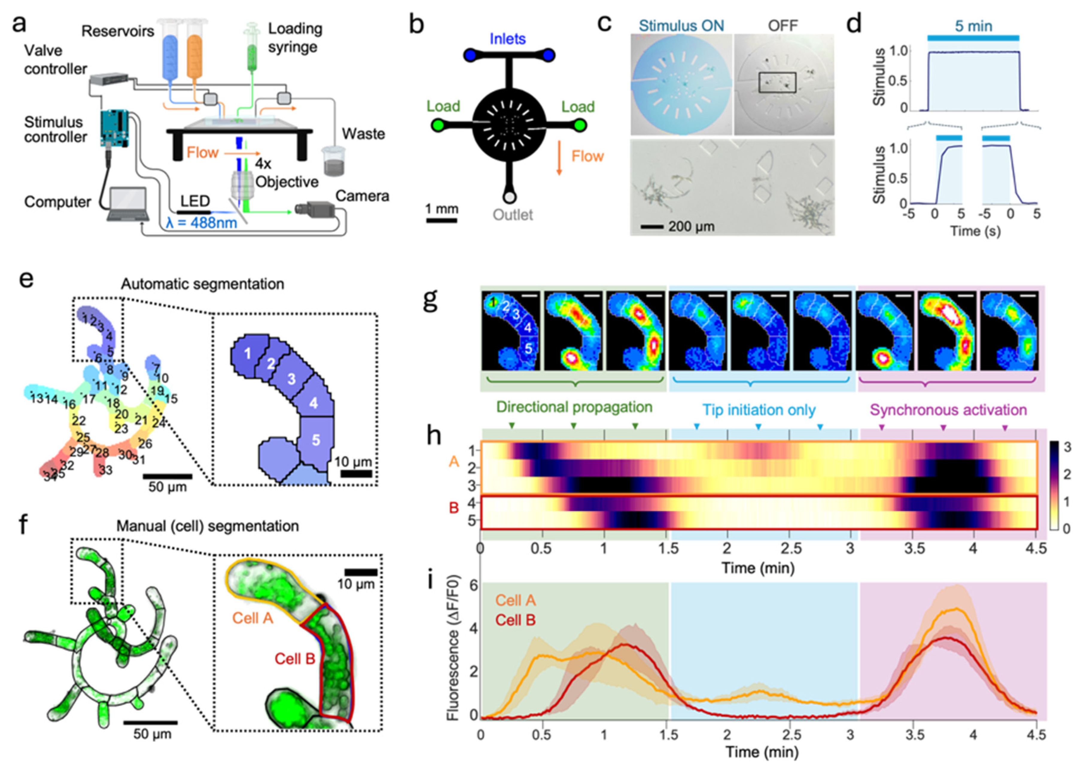
The automatic segmentation algorithm reduced data analysis time 10-fold, from upwards of an hour (for typical sized week-old protonemal plants) to ~5 min, removed bias implicit to manual segmentation, and identified physiologically-relevant subcellular regions that exhibited unique calcium dynamics, such as the apical CA* region versus the rest of the CA tip cell. These regions (for example, ROI #1 in Figure 2), exhibited basal calcium fluctuations prior to chitin addition characteristic of tip growth.

This study validated the use of microfluidic devices for studying chitin-induced Ca²⁺ waves at the plant, cell, and subcellular levels. The prolonged 30 min stimulation experiment most closely matched prior studies exposing moss protonemal tissues on agar pads to a sudden increase in chitin. Here, moss housed in microfluidic arenas demonstrated a similar rapid increase in cytosolic Ca²⁺ and comparable plant-wide oscillation interval (2 – 3 min interquartile range, vs. over 2 min interval on agar [3]). Before stimulation, growing apical regions of the caulonemal cells (CA* region) oscillated at a rate comparable to agar (2.4 – 2.6 per min vs. ~2 per min on agar [3]). We further characterized cell-type differences and found that while the frequency of chitin-induced waves was relatively consistent across all cell types, the waves in chloronemal and branch cells were slower and longer than caulonemal cells. Chloronemal tip cells exhibited Ca²⁺ waves and chitin-induced changes uniformly across the cell, with similar dynamics to those seen in the apical subcellular region of caulonemal tip cells, reflective of growth occurring in both tip cell types but more apically localized in the polarized caulonemal cells [8].

Chitin stimulation induced stereotyped, high amplitude calcium waves with a symmetrical rise and fall that scaled with wave duration, which varied four-fold across all conditions from about 30 to 120 s (mean 77 s; median 79 s; 65 – 91 s interquartile range). These wave dynamics did not correlate with wave interval, suggesting that wave initiation occurred by signaling processes separate from calcium levels. Oscillation intervals were consistent within each cell and ROI, at least over the time scale of an hour. Chitin-induced waves were initiated shortly after stimulus presentation, with an onset delay that varied several-fold (mean 32 s; median 24 s; 14 – 40 s interquartile range). These delays align with the timing of CERK1 activation by chitin and downstream MAPK phosphorylation [1]. Interestingly, initiation delays were longer after recent calcium activity, and shortest after quiescent periods, suggesting a “refractory period” in which components involved in calcium wave initiation accumulate or become sequestered during calcium activity and slowly recover responsiveness. Initiated waves followed their prescribed rise and fall and could not be terminated by removal of the stimulus, again suggesting a disconnect between the initiation (by chitin stimulation) and the progression of each calcium wave.

Circadian rhythms enable plants to manage daily cycles, such as the optimization of photosynthesis, stomatal opening, and metabolic processes to align with diurnal light and dark cycles, boost growth, and enhance fitness. The responsiveness of cells to external stimuli and internal signals is regulated by circadian rhythms though differential gene expression. In P. patens, cryptochrome CRY1 encodes when blue light affects gene expression by translocation into the nucleus, and clock genes such as CCA1 determine how strongly blue light is perceived by modulating blue-light receptors PHOT1/2, which implement phototropic responses at the cellular level [23]. Moss exhibit Ca²⁺ transients shortly after blue light [24], and we found that blue light excitation of the calcium sensor could directly trigger calcium responses under specific conditions.

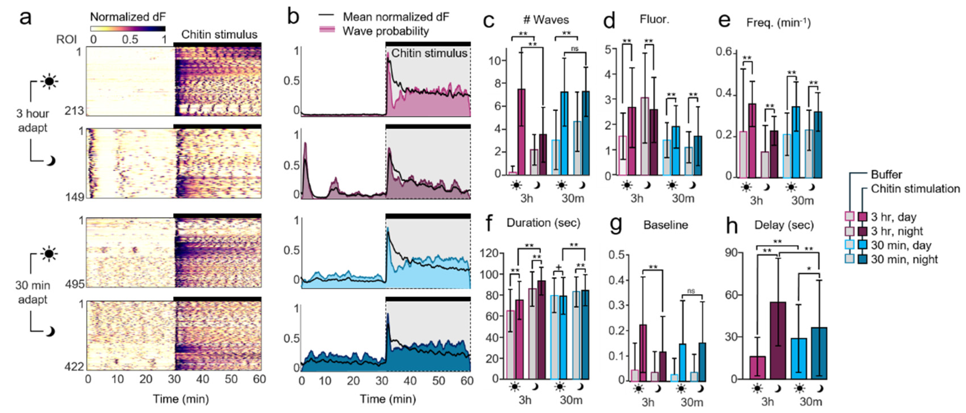
Light sensitivity motivated examination of different adaptation times in darkness prior to calcium recordings, as well as testing at various times during the day and night. The time of day affected calcium dynamics prior to chitin stimulation in long-adapted plants: in daytime, only caulonemal apical tip regions exhibited fluctuations in Ca²⁺ indicative of tip growth, while the rest of the cells remained silent. In contrast, plants stimulated at night exhibited an initial wave of Ca²⁺ during the first minute of imaging, reflecting sensitivity to blue light excitation. Following a brief quiescent period, spontaneous calcium waves propagated within and between adjacent cells, suggesting intercellular communication through plasmodesmata or apoplastic mechanisms [25]. Unlike long-adapted plants, short-adapted plants responded similarly at different times of day, suggesting that adaptation in the microfluidic device is required to observe sensitivity to circadian rhythms. Short-adapted plants also exhibited far more spontaneous Ca²⁺ activity prior to chitin stimulation, regardless of time of day.

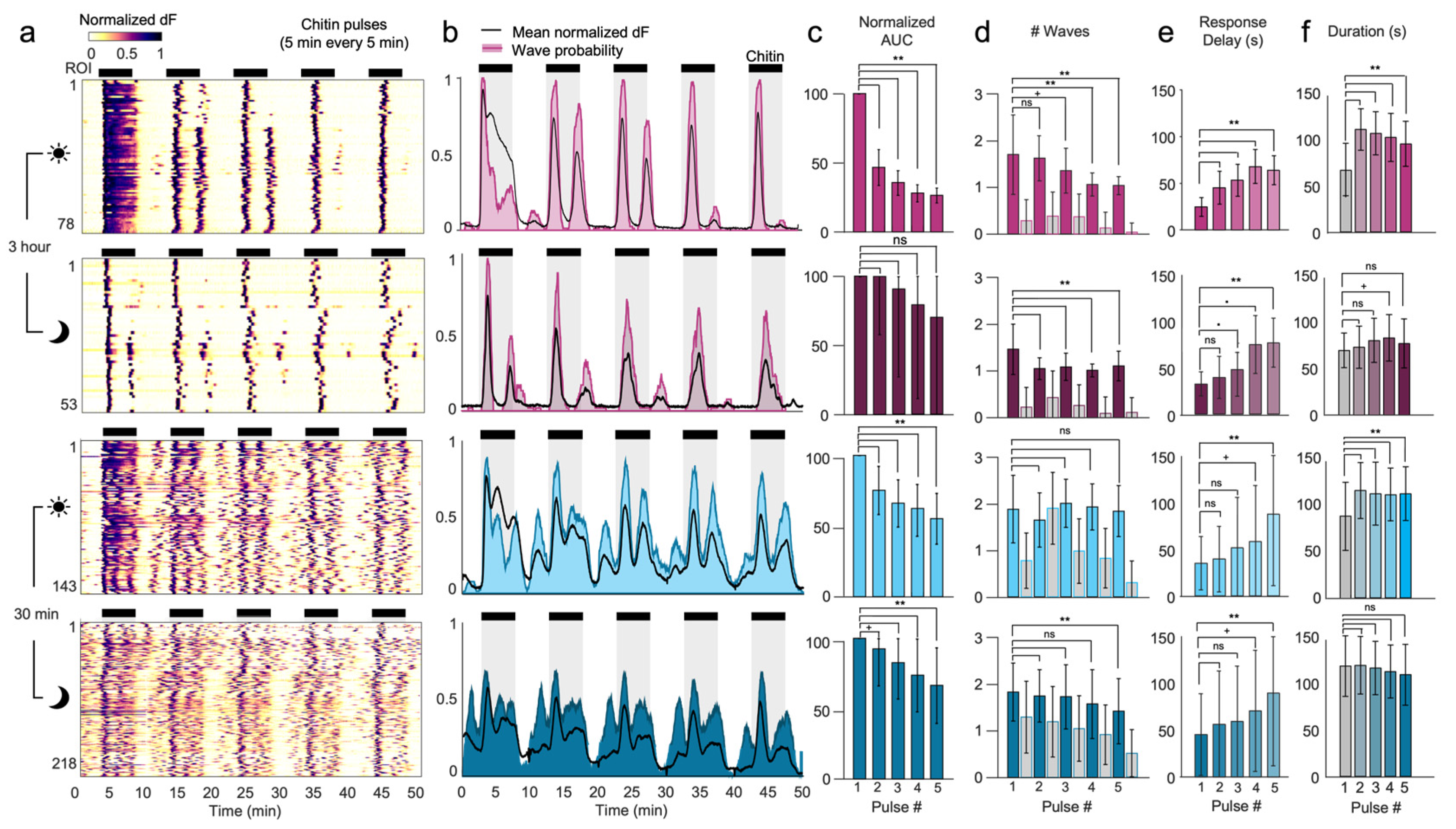
Repeated stimulation of living systems often elicits diminishing responses over time, such as adaptation of internal signals and habituation of organism behavior. A related memory phenomenon, priming, refers to the exogenous application of a substance to plants to enhance their natural defense responses and their tolerance to future stress presentations [26]. Because the microfluidic system can reversibly apply and remove chemical stimuli, we assessed for the first time whether calcium responses would adapt or change over multiple chitin stimulations. Indeed, stimulation with five cycles of 5 min chitin and 5 min of rest revealed a gradual response adaptation, with progressively lower calcium response levels, fewer calcium waves, longer wave intervals, longer onset delays, and decreased wave synchronicity. It is not yet clear how these history- and memory-dependent changes occur.

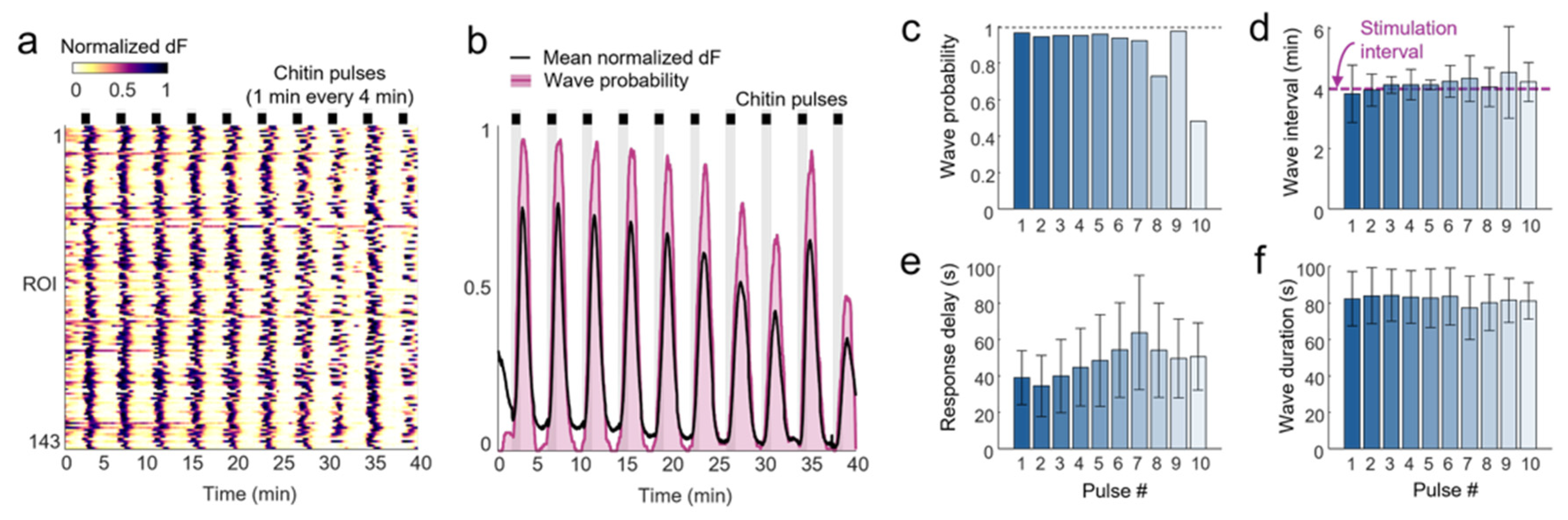
We also demonstrated a novel ability to entrain calcium oscillations to the prescribed frequency of chitin stimulation. As the sudden increase in chitin pulses elicited calcium waves in nearly all ROIs within 1 min, we investigated whether 1 min pulses of chitin could induce singular, synchronized calcium waves across plants. At a stimulation interval of 4 min, we found that nearly all ROIs exhibited single oscillations entrained at the same frequency as chitin stimulation. This external control of calcium wave frequency can be used to decode how wave frequency modulates gene expression.

In this study, all cells of the plant were stimulated equally and simultaneously by a uniform, high concentration of chitin oligosaccharides [3], representing a strong fungal attack. Beyond microfluidic control of chemical timing, devices with multiple inlets can control spatial chemical patterns by exploiting laminar flow physics [28,29]. Future experiments could stimulate a single cell within the plant by directing a narrow, micron-scale stream of chitin stimulus, and then trace signal propagation from the target cell across the plant. It will be interesting to observe the relation of calcium activity in adjacent cells when they are not exposed to the same external stimulus, and whether calcium waves propagate across cell boundaries under these conditions. This experimental setup may better resemble the initial encounter of a pathogen at a local point on the plant.

The characteristics of calcium waves, including symmetry and consistency, onset delays following stimulus addition, and inability to halt waves in progress by stimulus removal, all provide hints to the underlying signaling mechanisms. The lack of direct synchronization or calcium propagation across adjacent cells suggests signaling by other molecules. Dynamic mathematical models that produce simulated responses consistent with experimental data will be useful to investigate and identify these signals and to design perturbation experiments to further interrogate calcium signaling [27]. Together, this toolset should aid in the further study of calcium signaling in plants, including mechanisms of signal propagation, regulation of gene expression, and protection against external challenge.

4. Materials and Methods

4.1. Plant Material and Growth Conditions

All plant lines used in this study were derived from the moss Physcomitrium patens (Gransden strain). Moss lines were cultured in a Percival growth chamber at 25 °C under white light (Fluorescent Light bulbs cool white GE F17-T8 at ~100 µmol/sec/m²) and a 16 h/8 h light-dark cycle for 6-8 days before being used in experiments. Sub-culturing was done with an Omni Tissue Homogenizer (TH) set at half power and using 7 mm hard tissue Omni tip plastic probes. Plants were grown on cellophane disks (AA Packaging Limited, UK) placed on top of 1% agar WPi plant medium (described below) on 10 cm Petri dishes. One plate of one-week-old tissue was ground in 4 ml of water for ~10 sec. Two new plates were inoculated with 1 ml each, and the other two milliliters were sieved with a Falcon disposable cell strainer (70 µm pore size) to select for very small plants. The flow-through was placed onto two plates (1 ml each).

4.2. Solutions

The WPi plant medium was modified from {Ashton and Cove, 1977}: 1 mM MgSO₄· MgSO₄·7H₂O, 1 mM Ca(NO₃)₂·4H₂O, 4 mM KNO3, 89 µM Fe-EDTA, 1.84 mM KH₂PO₄, 9.9 µM H₃BO₃, 220 nM CuSO₄·5H₂O, 1.97 µM MnCl₂·4H₂O, 230 nM CoCl₂·6H₂O, 190 nM ZnSO₄·7H₂O, 168 nM KI, 100 nM NaMoO₄·2H₂O, pH 5.5. A 10X stock solution of 22 mg/ml chitin was prepared in water and stored at -20 degrees Celsius. The chitin stock was thawed and diluted in the media described above to a concentration of 2.2 mg/ml on the day of each experiment. The buffer solution was filtered through a 0.45 μm PES syringe filter (Genessee Scientific, USA; Cat#: 25-245) when creating the stimulus solution and passively before flowing into the microfluidic device to reduce the likelihood of aggregates entering the imaging area. The likelihood of aggregates increases with the length of time the stimulus solution is kept static. To allow the visualization and quantification of the fluid flow dynamics within the chamber and to verify the timing of stimulation, fluorescein was added to either the stimulus or buffer solutions for all experiments at a concentration of 0.1-1 μg/ml.

4.3. Microfluidic Device Design and Fabrication

To investigate dynamic plant-fungal interactions, we created a monolayer microfluidic device design capable of rapid, reversible switching between chemical stimuli. A chamber height of 35 or 50 μm was chosen to keep small moss plants withing the 50 μm depth of field of the fluorescent imaging setup. The design features two fluid inlet ports that connect to the imaging area via a T-shaped channel (Figure 1b) to enable the addition, removal, and spatial control of stimulus solution from the receptive field of the plants. Devices also feature two U-shaped traps inspired by (Sakai et al., 2019) aligned with each lateral loading port to locate plants centrally in the imaging area and provide support. The 3 mm diameter imaging area matched the microscope field of view and the surrounding support posts (100 x 200 μm) prevented collapse when plasma bonding. The device master molds were created by photolithography and soft lithography following methods previously described (Lagoy et. al., 2022). Briefly, a 35 μm or 50 μm layer of SU8 2035 photoresist (Microchem) was applied to a 4-inch wafer (University Wafer) and exposed through a 25,000-dpi photomask (CAD/Art Services) to generate a master mold. Polydimethylsiloxane (PDMS, Sylgard 184, mixed 1:10 by weight) was cast to create ~5mm thick microfluidic devices. Inflow, loading, and outflow ports were punched using a dermal punch (Miltex, 1 mm), then devices were cleaned and plasma bonded (Harrick PDC-32G, 18W, 45 sec) to a 25 x 75 mm glass slide. Assembled arenas were degassed in a vacuum desiccator for at least an hour before loading plant medium through the outlet port. This step ensures removal of air bubbles within the microfluidic channels prior to loading plants.

4.4. Experiment Setup

All solutions were filtered using 0.22 um PES syringe filters on the day of the experiment. Plant medium and chitin stimulus solutions were placed into 60 mL syringe reservoirs and covered with Parafilm. Microfluidic experiments were prepared by assembling fluid reservoirs and tubing as previously described (White et al., 2024; Lagoy et al., 2021). Inline 0.22 um Luer filters were connected below each reservoir and the 3-way Luer stopcock valve. Reservoirs were connected to the microfluidic device using tubing 0.020” Tygon microbore tubing connected to a blunt 23-gauge Luer stub adapter on one end and a ½” long 19-gauge stainless steel tube on the other end. Bubbles were removed from each fluid line before connecting to the degassed microfluidic device and filling it with plant medium (White et al., 2024). For each experiment, plants were randomly selected from the colony and placed in a dish of buffer solution. Plants were drawn into loading tubing with a 3-mL syringe, then gently injected into the arena using the loading ports and allowed to adapt to the microfluidic environment for 30 min to 3 h with continuous medium flow before imaging.

4.5. Automated Timelapse Imaging and Stimulation

Images were acquired using an inverted widefield epifluorescence microscope (Applied Scientific Instruments RAMM) with a 4x/0.28 NA objective (Olympus). Frames were acquired at 1 fps using a Hamamatsu Orca Flash 4.0 sCMOS camera mounted with a 1.0x c-Mount adapter. Binning was set to 2 to enhance the signal-to-noise ratio (SNR) of acquired signals for a spatial resolution of 0.345 pixels/μm (2.9 μm/pixel). A blue LED (Mightex GCS-470-50) excited GCaMP for 10 ms each acquisition frame. A 3-way solenoid valve (Bio-Chem Fluidics, PN: 075P2-S642) actuated by a ValveLink 8.2 (Automate Scientific) directed a stimulus or buffer solution into the microfluidic arena. Image capture, fluorescence illumination, and stimulus delivery were synchronized via digital trigger signals coordinated by an open-source system previously described in (White, et. al., 2023; Lawler, et. al, 2021). This system uses Micro-manager microscopy software (version 1.4.24) in streaming mode to acquire timelapse images and communicate experiment parameters by serial commands to an Arduino Uno microcontroller which coordinates digital trigger pulses (White, 2023).

Timelapse recordings of up to 60 minutes were conducted at room temperature (20-22 °C), beginning with plant medium flow. Chitin stimulation was introduced after 30 mins and persisted for 30 mins (Figure 2 and Figure 3), or chitin pulses were repeatedly introduced and removed for different durations and intervals (Figure 4 and Figure 5).

4.6. Structural Image Acquisition

After time-lapse recordings, microfluidic devices were moved to a Zeiss inverted microscope with an Axiocam 503 camera to identify individual cell borders. Plants were stained by flowing 0.1 µg/mL Direct Yellow 96 (Solophenyl Flavine 7GF5E) through the device for 30 min to label cell wall components. Brightfield and epifluorescence images were acquired at higher magnification (10x/0.3 NA) in Z-stacks with a 1.3 µm step size. Cell borders were manually outlined in FIJI (Schindelin, 2012) with the segmented line tool and validated between brightfield and stained images. These cell outlines provided the gold standard to evaluate the performance of the cluster generation algorithm and the initial number of ROIs per cell in the clustering algorithm, described below.

4.7. Image Processing Pipeline for Automated ROI Segmentation

4.7.1. Foreground-Background Detection

Regions of distinct calcium signal dynamics were automatically identified using an image processing pipeline depicted in Figure 6. First, raw TIFF stacks generated from the timelapse acquisition were cropped and processed with a FIJI macro (binaryMaskGeneration.ijm). The raw image stack was flattened by maximum z-projection and background subtraction was applied using radius values between 25 – 90 pixels depending on plant size. The resulting image was median filtered (radius = 2.5 pixels) to reduce noise and maintain contrast around the edges. To identify plant regions, an automatic threshold using the “Triangle” method was applied. Non-plant noise was removed by selecting pixel areas at least 200 pixels² and circularity larger than 0.9. Each binary mask was validated by manual inspection.

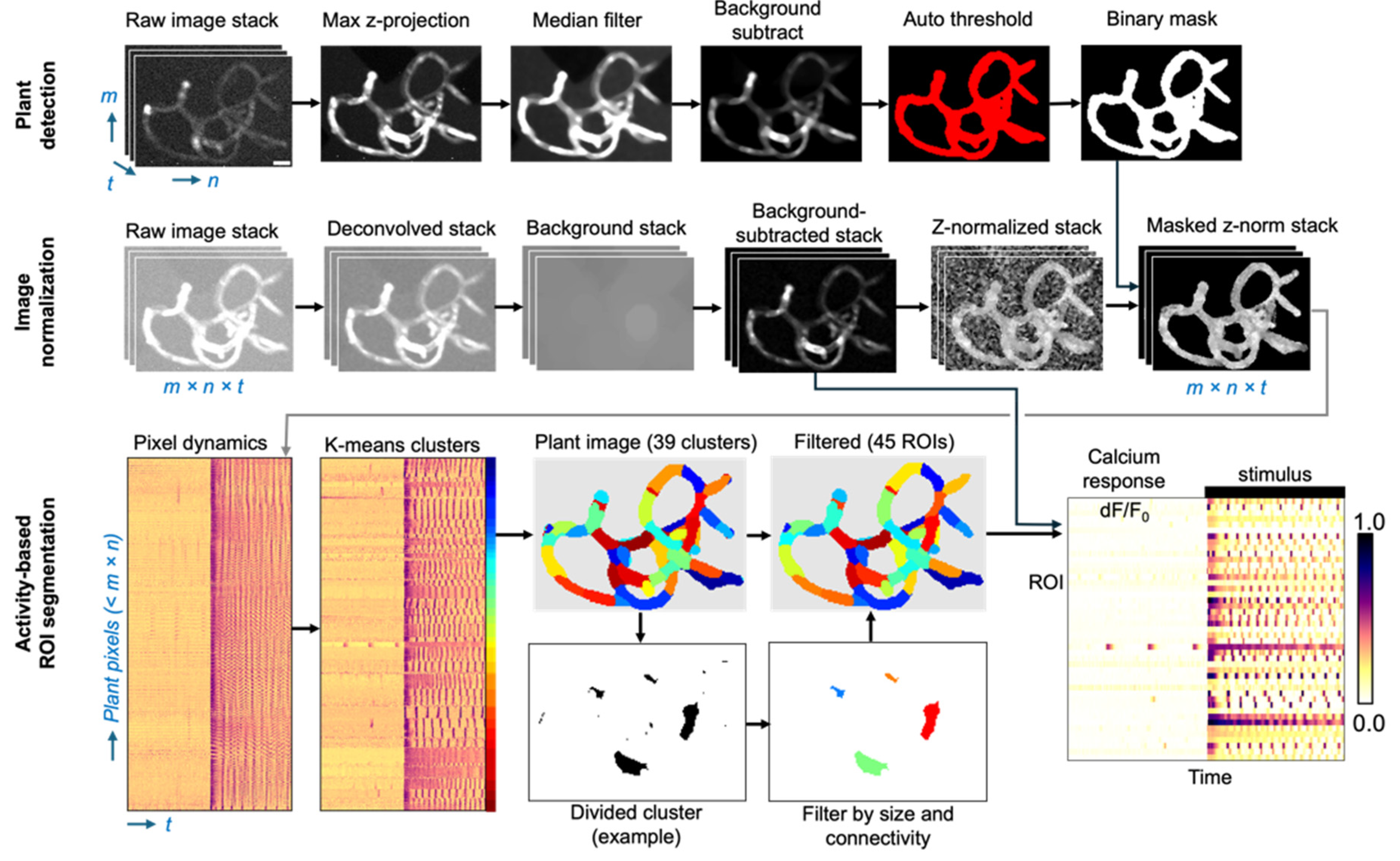
Figure 6. Automated plant ROI segmentation pipeline and data reduction. (top row) A binary mask is generated indicating plant pixels versus background pixels. The raw image stack (3D; m x n x t; in this example, 114 pixels wide x 158 pixels tall x 3600 frames) is reduced to an m x n binary mask image. (middle row) Calcium fluorescence image stacks are normalized to scale-independent Z-scores for each pixel, which equalize all pixels within a cell that respond with similar temporal dynamics. (bottom row) Data is flattened to a 2D matrix of each plant pixel Z-score over time (here, 5996 plant pixels x 3600 time points). K-means clustering grouped all pixels within 39 predicted clusters based on plant size (~150 pixel² per ROI). Clusters were reorganized to the plant geometry and filtered for size and connectedness. Filtered ROI numbers typically increase over initial cluster number. For example, a divided cluster is shown separated into four ROIs with noise pixels removed. Fluorescence intensity from the background-subtracted stack is integrated across each of the resulting 45 ROIs in this example, normalized to minimum intensity, yielding a reduced 2D dataset (45 ROIs x 3600 timepoints). .

Figure 6. Automated plant ROI segmentation pipeline and data reduction. (top row) A binary mask is generated indicating plant pixels versus background pixels. The raw image stack (3D; m x n x t; in this example, 114 pixels wide x 158 pixels tall x 3600 frames) is reduced to an m x n binary mask image. (middle row) Calcium fluorescence image stacks are normalized to scale-independent Z-scores for each pixel, which equalize all pixels within a cell that respond with similar temporal dynamics. (bottom row) Data is flattened to a 2D matrix of each plant pixel Z-score over time (here, 5996 plant pixels x 3600 time points). K-means clustering grouped all pixels within 39 predicted clusters based on plant size (~150 pixel² per ROI). Clusters were reorganized to the plant geometry and filtered for size and connectedness. Filtered ROI numbers typically increase over initial cluster number. For example, a divided cluster is shown separated into four ROIs with noise pixels removed. Fluorescence intensity from the background-subtracted stack is integrated across each of the resulting 45 ROIs in this example, normalized to minimum intensity, yielding a reduced 2D dataset (45 ROIs x 3600 timepoints). .

4.7.2. Fluorescence Image Correction and Normalization

To improve signal focus and reduce background fluorescence, each widefield image stack was deconvolved using a theoretical point spread function (PSF) assuming Abbe resolution limits (0.61 lambda / NA = 1.1 µm) using the ‘deconvolucy’ MATLAB command and ‘edgetaper’ to reduce ringing artifacts generated from iterative methods. We set the number of iterations to 10, which consistently generated smoother images and reduced the impact of out-of-focus blur without amplifying noise or introducing artifacts in the images (Ronneberger, 2008). This deconvolution step improved the outcome of the clustering algorithm, better matching ROIs to plant geometry.

GCaMP fluorescence (F_pixel) was obtained by subtracting background fluorescence from each pixel as follows. The previously generated binary masks were morphologically opened (MATLAB “imopen” function, with ‘disk’ structuring element and radius 15 pixels) to remove any structures smaller than 10 μm in diameter from the background images. The background images were then subtracted from the deconvolved image stack before quantification.

Fluorescence intensity is greatest in the center of each cell and lowest at the cell borders. Therefore, data were normalized to Z-scores per pixel before ROI detection, to group pixels by their dynamics irrespective of their time-averaged intensity. For each pixel, the mean intensity over time (µ) was subtracted from each time point (x) and divided by the standard deviation over time (σ), i.e. $Z=\left(x-\mu \right)/\sigma$. Z-normalized pixels are more uniform across each cell (Figure 6, middle row left). Next, background pixels were removed using the binary plant mask.

4.7.3. Data Reduction

To automatically identify contiguous pixel “regions of interest” (ROIs) with similar temporal dynamics, we first performed K-means clustering on a 2D matrix representation of the Z-normalized image stack. Each row of the 2D matrix represents a single pixel value over time (Figure 6, lower left). The clustering algorithm groups pixels into a pre-specified number of clusters given by the initial cell number estimated from manual observation. Where plants overlapped, the cluster number was increased to account for potential summation of fluorescence from both cells. Clustering used the distance metric “cosine” to maximize the similarity of pixels within the same cluster and the difference between separate clusters. We used the ‘OnlinePhase’ setting and 10 replicates with random initializations to guarantee a global minimization of distance metrics. The time course for each ROI was further reduced into 120 s windows surrounding the peak of ca2+ waves. Peaks were identified using the ‘findpeaks’ MATLAB function with a prominence threshold of 0.35 times the Median Absolute Deviation, chosen to capture both the spontaneous and chitin-driven oscillations. In contrast, standard deviation-based thresholding missed some spontaneous peaks or included false positive detections.

4.8. Statistical Analysis

Data are represented as the mean ± standard deviation (SD) unless otherwise noted, typically median and interquartile range (25 to 75 percentile) for non-normally distributed distributions. Non-responsive ROIs were excluded from categorization and quantification if the maximum increase in fluorescence (ΔF) within 5 minutes of stimulation was less than the baseline (F₀) fluorescence, typically lacked waves or oscillations to quantify. In comparison, the typical chitin-induced responses generated initial peaks around 250% ΔF/F₀. Sample sizes for each analysis (waves, ROIs, or plants) are reported in the figure legends. Statistics were performed using either a one-way ANOVA with Bonferroni’s correction for multiple comparisons, or two-tailed t-test using the Statistics and Machine Learning Toolbox in MATLAB (v. 2023a).

References

1. Bressendorff, S.; Azevedo, R.; Kenchappa, C.S.; Ponce de Leon, I.; Olsen, J.V.; Rasmussen, M.W.; Erbs, G.; Newman, M.A.; Petersen, M.; Mundy, J. An Innate Immunity Pathway in the Moss Physcomitrella patens. Plant Cell 2016, 28, 1328-1342. [CrossRef]
2. Ponce de Leon, I.; Montesano, M. Adaptation Mechanisms in the Evolution of Moss Defenses to Microbes. Front Plant Sci 2017, 8, 366. [CrossRef]
3. Galotto, G.; Abreu, I.; Sherman, C.; Liu, B.; Gonzalez-Guerrero, M.; Vidali, L. Chitin Triggers Calcium-Mediated Immune Response in the Plant Model Physcomitrella patens. Mol Plant Microbe Interact 2020, 33, 911-920. [CrossRef]
4. Zhang, H.; Yang, Q.; Wang, L.; Liu, H.; Zhang, D.; Duan, C.G.; Li, X. Moss-pathogen interactions: a review of the current status and future opportunities. Front Genet 2025, 16, 1539311. [CrossRef]
5. Ingle, R.A.; Stoker, C.; Stone, W.; Adams, N.; Smith, R.; Grant, M.; Carre, I.; Roden, L.C.; Denby, K.J. Jasmonate signalling drives time-of-day differences in susceptibility of Arabidopsis to the fungal pathogen Botrytis cinerea. Plant J 2015, 84, 937-948. [CrossRef]
6. Lecourieux, D.; Ranjeva, R.; Pugin, A. Calcium in plant defence-signalling pathways. New Phytol 2006, 171, 249-269. [CrossRef]
7. Cove, D.J.; Perroud, P.F.; Charron, A.J.; McDaniel, S.F.; Khandelwal, A.; Quatrano, R.S. The moss Physcomitrella patens: a novel model system for plant development and genomic studies. Cold Spring Harb Protoc. 2009 Feb;2009(2):pdb.emo115. [CrossRef] [PubMed]
8. Menand, B.; Calder, G.; Dolan, L. Both chloronemal and caulonemal cells expand by tip growth in the moss Physcomitrella patens. J Exp Bot 2007, 58, 1843-1849. [CrossRef]
9. Bascom, C.S., Jr.; Wu, S.Z.; Nelson, K.; Oakey, J.; Bezanilla, M. Long-Term Growth of Moss in Microfluidic Devices Enables Subcellular Studies in Development. Plant Physiol 2016, 172, 28-37. [CrossRef]
10. Bascom, C.S., Jr.; Winship, L.J.; Bezanilla, M. Simultaneous imaging and functional studies reveal a tight correlation between calcium and actin networks. Proc Natl Acad Sci U S A 2018, 115, E2869-E2878. [CrossRef]
11. Zhang, Y.; Zhang, D.; Huang, S.; Ye, N.; He, Y. Real-time calcium imaging in living plants. Trends Plant Sci 2023, 28, 1326-1327. [CrossRef]
12. Weigand, C.; Kim, S.H.; Brown, E.; Medina, E.; Mares, M., 3rd; Miller, G.; Harper, J.F.; Choi, W.G. A Ratiometric Calcium Reporter CGf Reveals Calcium Dynamics Both in the Single Cell and Whole Plant Levels Under Heat Stress. Front Plant Sci 2021, 12, 777975. [CrossRef]
13. Keinath, N.F.; Waadt, R.; Brugman, R.; Schroeder, J.I.; Grossmann, G.; Schumacher, K.; Krebs, M. Live Cell Imaging with R-GECO1 Sheds Light on flg22- and Chitin-Induced Transient [Ca(2+)]cyt Patterns in Arabidopsis. Mol Plant 2015, 8, 1188-1200. [CrossRef]
14. Sakai, K.; Charlot, F.; Le Saux, T.; Bonhomme, S.; Nogue, F.; Palauqui, J.C.; Fattaccioli, J. Design of a comprehensive microfluidic and microscopic toolbox for the ultra-wide spatio-temporal study of plant protoplasts development and physiology. Plant Methods 2019, 15, 79. [CrossRef]
15. Kozgunova, E.; Goshima, G. A versatile microfluidic device for highly inclined thin illumination microscopy in the moss Physcomitrella patens. Sci Rep 2019, 9, 15182. [CrossRef]
16. Whitesides, G.M. The origins and the future of microfluidics. Nature 2006, 442, 368-373. [CrossRef]
17. Albrecht, D.R.; Bargmann, C.I. High-content behavioral analysis of Caenorhabditis elegans in precise spatiotemporal chemical environments. Nat Methods 2011, 8, 599-605. [CrossRef]
18. Lagoy, R.C.; Larsen, E.; Lawler, D.; White, H.; Albrecht, D.R. Microfluidic Devices for Behavioral Analysis, Microscopy, and Neuronal Imaging in Caenorhabditis elegans. Methods Mol Biol 2022, 2468, 293-318. [CrossRef]
19. White, H.; Kamara, V.; Gorski, V.; Busby, M.; Albrecht, D.R. Automated Multimodal Stimulation and Simultaneous Neuronal Recording from Multiple Small Organisms. J Vis Exp 2023. [CrossRef]
20. Chen, Y.; Song, X.; Ye, S.; Miao, L.; Zhu, Y.; Zhang, R.G.; Ji, G. Structural insight into enhanced calcium indicator GCaMP3 and GCaMPJ to promote further improvement. Protein Cell 2013, 4, 299-309. [CrossRef]
21. Karapetyan, S.; Dong, X. Redox and the circadian clock in plant immunity: A balancing act. Free Radic Biol Med 2018, 119, 56-61. [CrossRef]
22. Chiso, K.; Yamashino, T.; Suzuki, R.; Gans, T.; Trogu, S.; Hughes, J.; Aoki, S. Light responses during early day phases of CIRCADIAN CLOCK ASSOCIATED 1 (CCA1) and PSEUDO-RESPONSE REGULATOR (PRR) homologous genes in the moss Physcomitrium patens. Photochem Photobiol 2025, 101, 762-770. [CrossRef]
23. Imaizumi, T.; Kadota, A.; Hasebe, M.; Wada, M. Cryptochrome light signals control development to suppress auxin sensitivity in the moss Physcomitrella patens. Plant Cell 2002, 14, 373-386. [CrossRef]
24. Russell, A.J.; Cove, D.J.; Trewavas, A.J.; Wang, T.L. Blue light but not red light induces a calcium transient in the moss Physcomitrella patens (Hedw.) B., S. & G. Planta 1998, 206, 278-283. [CrossRef]
25. Choi, W.G.; Miller, G.; Wallace, I.; Harper, J.; Mittler, R.; Gilroy, S. Orchestrating rapid long-distance signaling in plants with Ca(2+) , ROS and electrical signals. Plant J 2017, 90, 698-707. [CrossRef]
26. Sahoo, L.; Swain, B.; Yadav, D. A review on different priming strategies to mitigate abiotic stress in plants. Discover Applied Sciences 2025, 7. [CrossRef]
27. Bose, J.; Pottosin, II; Shabala, S.S.; Palmgren, M.G.; Shabala, S. Calcium efflux systems in stress signaling and adaptation in plants. Front Plant Sci 2011, 2, 85. [CrossRef]
28. Larsch, J.; Ventimiglia, D.; Bargmann, C.I.; Albrecht, D.R. High-throughput imaging of neuronal activity in Caenorhabditis elegans. Proc Natl Acad Sci U S A 2013, 110, E4266-4273. [CrossRef]
29. Tourovskaia, A.; Figueroa-Masot, X.; Folch, A. Long-term microfluidic cultures of myotube microarrays for high-throughput focal stimulation. Nat Protoc 2006, 1, 1092-1104. [CrossRef]
Figure 1. Microfluidic system for plant stimulation and calcium imaging. (a) Diagram of image acquisition setup. LED, light-emitting diode. (b) Diagram of the microfluidic device and flow path. Fluid flows from one of two reservoirs (stimulus or plant medium) via inlets (blue) to the outlet. Plants are loaded from either of two side ports (green). (c) Fluid in the arena can be switched rapidly and reversibly between the stimulus (blue) and plant medium (clear) solutions, exposing multiple plants to different chemical environments (inset). Here, blue dye was used to visualize the stimulus solution. (d) Switching between solutions is rapid and repeatable. Dye intensity plots show the mean ± SEM of five repeated pulses, each 5 min in duration. (e) An automated algorithm generates regions of interest (ROIs) by clustering pixels with similar fluorescence dynamics (see Methods, Figure 6). ROIs represent cells or subcellular regions. (f) Brightfield image of the same plant as in (e), manually segmented along cell wall boundaries. Typical cells are represented by 1 – 3 ROIs: cell A (orange) is represented by ROIs 1-3 and cell B (red) by ROIs 4,5. The green fluorescence overlay represents cell wall staining using Direct Yellow 96 and chloroplast autofluorescence. (g) Timelapse frames (30 sec interval) depicting calcium fluctuations in the five automatically-generated ROIs underlying cells A and B. Scale bars = 10 μm. (h) Heatmaps of the ROI-averaged fluorescence values which clearly demonstrate different calcium wave behaviors: (1) propagating from the apical tip in the basal direction (green), (2) tip initiation without propagation (blue), and (3) synchronous activation of all ROIs and dissipation. (i) Averages for cells A and B show similar patterns, but obscure subcellular propagation, seen as increased SD amplitude (shading).
Preprints 194427 g001
Figure 4. Repeated chitin pulses elicit repeated calcium waves. (a) Normalized heatmaps of plant ROIs during five 5-min chitin stimulation pulses. Plants were adapted in the microfluidic device for 3 h or 30 min and imaged during daytime (dawn-to-dusk) or nighttime, as indicated. Calcium fluorescence is shown normalized to the minimum and peak intensity per ROI. (b) Mean ROI responses are shown as normalized fluorescence intensity (black line) or as instantaneous probability of a calcium wave over time (shading). Black bars and grey shading represent chitin addition. (c-f) Comparison of calcium wave dynamics throughout the 5 stimulus additions. Data represent (c) the normalized area under the curve (AUC) of each stimulus repetition normalized to the response to the first stimulus pulse; (d) the average number of waves exhibited per ROI per 5-min time period; (e) the response latency between the five chitin additions and the initiation of the first chitin-induced wave (above 10% of maximum prominence); and (f) calcium wave duration (above 10% of maximum prominence, i.e. FW10). **, p<0.0001; *, p<0.001 for buffer vs. stimulus or specified comparison; +, p<0.0001 compared with buffer, 3h adapt, daytime condition. Data represent mean and SD, n = 53 – 218 waves from 2 – 5 plants.
Preprints 194427 g004
Figure 5. Calcium wave frequency is driven by chitin stimulation frequency. (a) Normalized heatmap of plant ROIs during ten 1-min chitin stimulation pulses every 4 min. The plant was adapted in the microfluidic device for 1 h before imaging. Calcium fluorescence (dF) is normalized to the minimum and peak intensity per ROI. Data represents n = 143 ROIs from one plant. (b) Mean ROI response shown as normalized fluorescence intensity averaged across all ROIs per condition (black line) or as probability of a calcium wave over time (shading). Bars and shading represent chitin pulses. (c-f) Comparison of calcium wave dynamics across 10 repeated stimulus pulses, including (c) the probability of eliciting a calcium wave; (d) intervals between calcium waves; (e) response delay between chitin addition and calcium fluorescence rise (to 10% of maximum); and (f) calcium wave duration. Data represents mean and SD, n = 71 – 146 waves per pulse.
Preprints 194427 g005
Disclaimer/Publisher’s Note: The statements, opinions and data contained in all publications are solely those of the individual author(s) and contributor(s) and not of MDPI and/or the editor(s). MDPI and/or the editor(s) disclaim responsibility for any injury to people or property resulting from any ideas, methods, instructions or products referred to in the content.
Copyright: This open access article is published under a Creative Commons CC BY 4.0 license, which permit the free download, distribution, and reuse, provided that the author and preprint are cited in any reuse.
Prerpints.org logo
Preprints.org is a free preprint server supported by MDPI in Basel, Switzerland.
Subscribe
Disclaimer
Terms of Use
Privacy Policy
Privacy Settings
© 2026 MDPI (Basel, Switzerland) unless otherwise stated