
Submitted:
14 January 2026
Posted:
15 January 2026
You are already at the latest version
Abstract
In recent years, the architectural design process has experienced significant advance-ments due to computational design, which has enabled the real-time exploration of design alternatives based on parametric modeling. In this context, gaining a deeper understanding of how natural ventilation operates within buildings can support deci-sion-making, potentially reducing the need for wind tunnel tests and computational simulations. This paper presents an effort to determine the flow patterns of natural ventilation in indoor environments under specific conditions, using an experimental setup comprising five configurations analyzed comparatively against a control sample. An idealized and simple flow visualization technique was proposed to assist the anal-ysis. By following scientific methodologies and employing both computational and wind tunnel techniques in a complementary manner, satisfactory inferences were ob-tained. The results indicate that the diagonal positioning of openings substantially ac-celerates wind speed in indoor environments, making this design strategy more effec-tive than simply adding additional openings when the goal is to increase air speed and indoor air renewal.
Keywords:
natural ventilation
; indoor environment
; wind-tunnel
; CFD
; simulation-based architectural design
1. Introduction
Since the publication of Performative Architecture: Beyond Instrumentality [1], professionals have been increasingly concerned with improving performance in architectural design. This concern has long been present in the works of architects such as Antoni Gaudí, Heinz Isler, and Frei Otto. However, according to contemporary authors, the widespread availability of software now facilitates the incorporation of performance analysis results, particularly in the areas of structural and environmental behavior, during the early stages of design. Simulation processes in architecture are not new, and their development since the 1960s was accelerated by computational insights presented by Sutherland [2] and Eastman [3]. In the 1990s, many simulation methods were inspired by biological processes, aiming to achieve responsive behavior in algorithms used to address design problems in different scenarios [4]. Since then, simulation-based architectural design has significantly influenced the environmental and structural performance of numerous buildings in the first two decades of the twenty-first century [5].
In general, well-defined variables are easier to measure, depending on recursive behavior, such as solar trajectory. However, design strategies that combine other variables, like radiation or air movement, were explored in seminal works on bioclimatic zones by Olgyay [6] and Givoni [7,8]. From these authors, natural ventilation emerged as a design alternative for regulating thermal mass in buildings. While there is an agreement among researchers that cross-ventilation offers benefits within buildings [9,10], there is still uncertainty and sometimes incorrect strategies for enhancing its effects through openings. Even though parallel windows, for instance, improve internal ventilation levels, their placement can significantly affect wind speeds, flow direction, and overall performance, and this sensitivity to geometric configuration is consistent with findings from studies on re-entrant bays in high-rise buildings [11] and from analyses of single-sided façade ventilation [12], which show that small variations in façade geometry can enhance or hinder natural ventilation by altering pressure distributions and inducing unwanted recirculation zones.
The description of natural ventilation phenomena within buildings is not recursive and often exhibits chaotic behavior. However, more insights have been gained through various models, graphs, and Computational Fluid Dynamics (CFD) analysis in air conditioning and Heating, Ventilation, and Air Conditioning (HVAC) systems to determine thermal areas and noise increases [13]. In architecture, the inference of natural ventilation throughout the design process commonly relies on weather files, while design science employs instructional strategies with test configurations in a wind tunnel and computer simulations from an ontological perspective [14,15]. The combination of wind tunnel measurements and numerical simulations was used in a landmark approach to analyze how wind direction, wind speed, and opening configuration influence cross ventilation in buildings with large openings, elucidating complex indoor flow patterns and proposing more accurate discharge coefficients to adequately represent the real airflow [16]. Recent studies have used these findings to predict the effects of cross-ventilation on indoor environments to inform the design process [17].
As an innovative aspect, this paper presents an effort to understand the behavior of natural ventilation in indoor environments under specific conditions, using an experimental design comprising five configurations compared to a control sample. These treatments aim to replicate the design strategies of cross-ventilation, which, in summary, involve the use of parallel openings to facilitate air circulation in the environment. Additionally, a straightforward flow visualization technique was proposed to aid in comprehending the flow pattern inside the physical prototype. Both CFD simulations and wind tunnel tests complemented each other in achieving a high level of inference about the flow field.
As an innovative contribution, this paper seeks to understand the behavior of natural ventilation in indoor environments under specific conditions, using an experimental design comprising five configurations compared with a control sample. These treatments aim to replicate cross-ventilation design strategies that, in summary, involve the use of parallel openings to facilitate air circulation within the environment. Additionally, a straightforward flow visualization technique was proposed to aid in understanding the flow patterns inside the physical prototype. Both CFD simulations and wind tunnel tests complemented each other, enabling a higher degree of inference regarding the behavior of the flow field.
2. Related Work
In recent years, the architectural design process has experienced significant advancements resulting from computational design, which has enabled the real-time exploration of design alternatives based on parametric modeling. The integration of these tools with CFD (Computational Fluid Dynamics) wind simulations supports the decision-making process, ranging from geometric exploration and the simultaneous assessment of ventilation effects [18,19] to the evaluation of solution quality in Building Information Modeling (BIM) environments [20]. Although most applications used in architectural design do not offer native CFD capabilities, it is possible to correlate other properties, such as preliminary estimates of thermal performance, with CFD-based ventilation assessments to reduce heat gain in buildings [21].
The study of ventilation in conjunction with cooling systems has been the subject of various research efforts aimed at developing passive cooling strategies that do not rely on mechanical systems [22]. CFD simulations have provided insights into roof elements used to lower indoor temperatures, including the impact of ventilation towers [23] and chimneys in facilitating ventilation [24,25], the aerodynamics of dome geometries [26], and the influence of balcony depth [27]. Recent numerical studies have further shown that the configuration and relative positioning of openings strongly influence indoor airflow patterns and cross-ventilation efficiency [28]. Similar simulations have enabled researchers to quantify the extent to which architectural elements obstruct or promote cross-ventilation through increased air movement. Factors such as wall placement can be crucial in improving indoor airflow distribution [29], as well as the geometry and positioning of windows, which enhance wind penetration into indoor environments [30,31].
With a similar focus, both numerical and experimental investigations have sought to characterize natural ventilation in indoor environments by analyzing the building envelope [32]. Studies combining CFD simulations with experimental measurements have highlighted the importance of experimental validation to reliably capture indoor airflow behavior and reduce uncertainties associated with numerical predictions [33]. Design alternatives have been proposed for office buildings based on on-site measurements and simulation processes [34,35], although disparities persist between the natural ventilation strategies conceived during design stages and their actual operation in constructed buildings [36]. In school buildings, efforts have highlighted the benefits of cross-ventilation, primarily regarding window orientation and opening percentages [37,38,39]. Conversely, adverse effects of natural ventilation have been reported in hospital environments [40,41]. Other research has used CFD simulations to predict airflow behavior for contaminant removal [42], enhance livestock and poultry welfare [43,44], and improve the quality of certain crops [45].
Validating computer simulations of natural ventilation effects typically involves comparing CFD results with wind tunnel experiments to confirm accurate measurements of external flow phenomena [46]. Macro-scale effects of cross-ventilation and pollutant dispersion are addressed in [47,48]. Additional studies have proposed various parametric design interactions to evaluate the sensitivity of CFD applications [49,50,51,52], and supportive tools have been developed to enable rapid manual estimations of heat loss resulting from natural ventilation processes [53]. As the use of natural ventilation as a design strategy continues to expand [54], the need for scientific research that offers a more precise understanding of the aerodynamic behavior of indoor cross-ventilation becomes increasingly evident.
3. Materials and Methods
3.1. Experimental Setup
Natural cross ventilation through a low-rise building was considered to investigate both experimentally and numerically the flow mechanisms and their impact on human comfort inside the room. The cross-ventilated building model used in this research was originally created for this purpose and has the following dimensions: 300 × 450 × 150 mm (L × W × B). The height (B) of the building will be used, from now on, to nondimensionalize the main descriptive variables of this problem. This rectangular structure has six ventilation windows arranged symmetrically with respect to the model centerline, with three ventilation openings on the front façade and three ventilation exits on the rear façade. All openings have the same dimensions, w × h = 120 × 75 mm, and the horizontal distance between openings is 22.5 mm. Figure 1 shows a schematic view and dimensions of the WDN-CV model used in this study.
For testing the effect of different cross-ventilation patterns, all the openings and exits could be closed independently. Depending on the number and the location of windows, the following cross-ventilation cases were considered:
- Control sample: all windows open
- Treatment 1 (Diagonal): windows 2, 3, 4, and 5 closed
- Treatment 2 (Face-to-face): windows 2 and 5 closed
- Treatment 3 (Face-to-face): windows 4 and 6 closed
- Treatment 4 (Face-to-face): windows 1 and 3 closed
- Treatment 5 (Diagonal): windows 3 and 4 closed
The physical building model was built with 3 mm transparent acrylic mate-rial to facilitate the flow characterization inside the room as well as to assure transparency and access of the anemometer probe for collecting velocity profiles.
The prototype was built for measurements in a wind tunnel to verify the behavior of air movement internally. Its dimensions are proportional to the full-scale built environment of 54 m² (9 x 6 m) and 3 m ceiling height in 1:25 scale. The basic configuration features only window openings, six in total, three on each side, in opposite positions, to study cross ventilation. In addition, these openings cut out in the prototype do not fully represent the authentic frames existing in these buildings due to the re-ductions imposed by experimentation and simulation.
3.2. The Wind-Driven Natural Cross Ventilation (WDN-CV) Model
Experimental measurements and flow visualization were carried out in the open circuit wind tunnel (WT) at the Experimental Aerodynamics Research Center (CPAERO) of the Federal University of Uberlândia, Brazil [55,56]. The small wind tunnel, named TV-60-Zephyr, is an open circuit with a closed working section. Flow momentum is created by a rotor with 12 blades driven by a 25 Hp electric engine. The maximum air speed in the tunnel test section (0.6 m × 0.6 m × 1.0 m) is approximately 30 m/s, with minimal blockage and moderate-to-low turbulence intensity (0.15–0.8% along the speed range). With easy access to the working section, this WT is also equipped with a three-component dynamic force/moment balance, an interchangeable multiport simultaneous pressure scanning system with two Pitot tubes, and vertical and transversal home-built rakes for speed and pressure measurements (not used in this work). Boundary layer (BL) profiles are gathered with a home-built BL mouse. Very low-speed flows (low Reynolds numbers) are tested in this WT, supporting applications such as low-speed foils, flow over simplified vehicles and bodies, and fundamental fluid mechanics research [57,58,59].
The WDN-CV model was placed at a location of 2.35 B from the inlet of the test section, with a blockage ratio of 19%. This value is above the recommended practice for natural ventilation studies. According to Jewel et al. [60] and Matsumoto, Labaki and Caram [61], it is one of the limitations of this study, and the final data depend on this blockage ratio (no corrections were applied). However, it is believed that due to the low speed and reasonable stability and uniformity of the incoming flow inside the wind tunnel, the results are reliable and allow for sound inferences and understanding of the flow inside the building. It is also important to emphasize that the same configuration was replicated in the CFD analysis, which helps ensure the consistency of the chosen approach.
For all tested configurations, the reference mean wind velocity (Uref) was 5 m/s, measured with a Pitot tube connected to a M200-Kimo® pressure transducer with a resolution of 0.1 Pa and readout accuracy of ±0.2%. Temperature inside the test chamber was measured with a Minipa® MT-455A digital thermometer with an MTK-01 thermocouple, with a resolution of 0.1°C and readout accuracy of ±0.5%. The WDN-CV model placed inside the test section is shown in Figure 2.
The main governing parameter of this type of study is the Reynolds number Re= (ρUrefB)/μ, where ρ is the air density (kg/m3) and μ is the dynamic viscosity (Pa. s), which based on the height (B) of the prototype building is on the order of 50.000.
3.3. Inflow Conditions and Boundary Layer Characterization
Due to the nature of this approach, the velocity inlet conditions were not corrected for atmospheric boundary layer (bl), i.e., the upstream section was completely clean. The vertical profile of the mean wind velocity was placed at 1.23 B ahead of the building model. The boundary layer measurement was achieved by using a Dantec Dynamics anemometry system (Streamline PRO 90CN10) with hot-wire CTA (constant temperature anemometer) probes (55P11) used for measuring the u-velocity component with the test-model in the test-section. The building reference height (href) of 150 mm was adopted, and the reference mean wind velocity (Uref) was 5 ms-1. The dimensionless mean streamwise velocity (U(z)) and turbulence intensity (I%) profiles are shown in Figure 3:
For all measurements performed with the hot-wire anemometer, the sampling rate was set to 8192 Hz over an 8-second time-averaging period to obtain statistically stationary data, as shown in the sample in Figure 4.
3.4. Measurement
The experiments in the wind tunnel were carried out to measure the velocity profiles, to evaluate the flow pattern, and to determine the ventilation flow rate through the windows. The u-velocity component was measured along a horizontal line inside the room at mid-height, from front window no. 2 to rear window no. 5, as described in Figure 5.
If the flow reached its steady motion, and no reversal flow was identified in the windows on the leeward wall, hot-wire multi-point measurements for u-velocity were taken for the inlet windows 1-3 (windward wall) and outlets windows 4-6 (leeward wall) on a cross-configuration at mid-location of each half-window part, as seen on Figure 6. Since the volumetric flow rate through the inlet and outlet has been almost constant i.e., equal in magnitude, the mass flow is conserved, as expected. In this analysis the volumetric flow rate (Q= ∑_1^5 A_i u_i) was calculated directly.
3.5. Flow Visualization by Inferences from Particle’s Movement
Due to the expected strong influence of cross ventilation inside the room, a simple qualitative flow visualization technique was proposed in this study. Inside the model, the floor was divided into four zones, and in these areas small, lightweight polystyrene balls (approximate density of 13.8 kg/m³) with an average diameter of 2.4 mm in different colors (yellow, orange, blue, and pink) were used, as shown in Figure 7. Afterwards, CFD simulation will be used to enhance the main observations through comparison in two horizontal planes: one at mid-window height and another close to the floor, where the main movements of the polystyrene balls occur due to the crossflow in the physical experiment.
By analyzing the movement of the polystyrene balls over time, it was possible to establish a pattern inside the room associated with the mean flow. This simple flow visualization approach was useful for understanding how the flow changes according to the opening and closing of the windows across the different settings. Moreover, based on the displacement of the particles and the mixing between the colors, inferences about the quality of the flow experienced by occupants could be made for the different configurations studied.
4. Numerical Modeling
The same wind-driven natural cross-ventilation (WDN-CV) model configuration was simulated using the commercial CFD code Fluent® R22. The basic assumptions for the CFD simulation include a three-dimensional, fully turbulent, incompressible flow. The internal and external flows were modeled using the Realizable k-e turbulence model, a well-established approach in natural ventilation research whose limitations and restrictions have been documented in several studies. The CFD code employed the Finite Volume Method (FVM) and the Semi-Implicit Method for Pressure-Linked Equations (SIMPLE) velocity–pressure coupling algorithm, with second-order upwind discretization as recommended in the literature. The governing equations will not be repeated here but can be found in Ansys [62].
Even though different turbulence models have been used for WDN-CV simulations, and that some improved models can lead to better results [63], the main goal of this approach was to use a traditional and well-validated k-ε model to obtain the average flow field and maintain a focus on flow analysis. According to the work of [64], the flow around a building (a bluff body) is fully turbulent when ReB > 2 × 10^4, whereas the airflow discharging through a window (an opening) becomes turbulent when ReW > 300. In this study, the flow around the building is governed by a Reynolds number of approximately 50,000, while in the openings it is close to 23,000. Therefore, the flow was considered fully turbulent.
4.1. Wind Tunnel Specification
A schematic view of the computational domain is presented in Figure 8. As mentioned, the width, length, and height are 0.60 m × 0.60 m × 1.0 m, respectively, reproducing the actual wind tunnel test section.
The inlet boundary condition used in the simulations was based on the actual wind tunnel experiment. During the experimental campaign, ambient pressure (Pa), temperature (°C), and relative humidity (%) were recorded using a SUNROAD® FR500 digital barometer with a resolution of 0.1 hPa, a Minipa® MT-455A digital thermometer with an MTK-01 thermocouple with a resolution of 0.1°C, and a mini digital weather station with a resolution of 1% RH. The averaged values used in this work were p∞ = 98,000 Pa, T∞ = 25°C, and RH = 50%, which resulted in an air density of 1.18 kg/m³ used in all simulations.
Zero static pressure was applied at the outlet plane, defined as outflow, representing the atmospheric exit of the test section. For the ground surface, the building model, and the wind tunnel walls, enhanced wall functions were used.
4.2. Mesh Sizing and Grid Approach
The grid spacing is an important parameter not only for ensuring accurate results but also for achieving a good balance between reliable data and optimal meshing effort and computational time. Four different mesh sizes were evaluated to meet these goals. The computational simulations used unstructured tetrahedral meshes with the global grid parameters presented in Table 1.
Mesh #3 is shown in Figure 9, with a refinement detail on the windward wall near the wind tunnel floor. As observed, the smallest grid spacing was applied near the walls (both inside and outside the building) to properly capture the boundary effects on the flow field. This mesh refinement near the wall followed the guidelines for the RANS approach, in which y+ (the nondimensional distance of the first grid point from the solid surface) was kept between 1 and 30.
5. Validation of Numerical Approach
A validation approach was necessary to demonstrate the reliability of the data as well as the limitations of the realizable k-ε turbulence model used in this study. A set of validation checks was performed, including the influence of grid spacing on the results, measurements of u-velocity at the inlets and outlets to verify the volumetric flow rate, u-velocity distribution along a horizontal line inside the building, and wind tunnel boundary layer measurements. These results are presented in sequence.
Figure 10 illustrates the evolution of the ventilation rate (m³/s) as a function of grid size. The discrepancy in this variable between meshes #4 and #5 was below 1 percent. The flow fields obtained with meshes #4 and #5 were also quite similar, as were the residuals. Based on these results, the mesh used for subsequent analyses was the one with 2.7 million elements.
The comparison of the non-dimensional velocity distribution along a horizontal line located at mid-height from window 2 to the corresponding rear window 4, as shown in Figure 5, is presented in Figure 11. In this case, all other windows are open, representing the control configuration.
Despite the discrepancies in velocity values in the middle of the building, the peak value at the entry location is nearly reproduced, as is the recovery of speed at the exit opening. This indicates that the volumetric flow rate is well captured at both the front and rear windows, as will be discussed later.
The comparison with the wind tunnel boundary layer is shown in Figure 12. The boundary layer was measured at an upstream location of 1.23 H, starting from 1 mm up to 100 mm into the flow field. As seen in Figure 12, the numerical velocity profile differs slightly from the experimental data, which is associated with the turbulence model used in the present study (Realizable k-ε). This trend has been previously observed and discussed in the works of Blocken, Carmeliet, and Stathopoulos [65], and Ouyang and Haghighat [66], and is related to artificial diffusion in the numerical approach, which causes the wind flow to slump near the ground. There is also a slight difference in the peak values of u(z)/Uref, resulting in approximately 16 percent deviation.
It is important to emphasize that the objective of this work is not to perform an in-depth study of the variables that influence the problem, but rather to reproduce in a numerical model the flow patterns observed in the physical experiment. To achieve this goal, no changes or corrections were applied to the original flow, and therefore the results retain the limitations and restrictions inherent to both the experiment and the numerical model.
Finally, the last validation check involved the direct calculation of the volumetric flow rate through the inlets and outlets and its comparison with the CFD data. These results are presented in Table 2. As discussed in Figure 10, the flow at the inlets and outlets shows satisfactory agreement, which is confirmed by the volumetric flow rate values. As expected, the largest discrepancies (approximately 8 percent) occur at the windward windows (W1, W2, and W3) due to differences in the incident velocity.
At the leeward windows (W4, W5, and W6), the flow velocity is recovered as previously shown in Figure 10, resulting in a good match in the flow rate, with deviations on the order of 2 percent. An important observation is that the middle outlet window (W5) carries a smaller flow rate, while the flow remains symmetric through W4 and W6.
On the leeward windows (W4, W5, and W6), the flow velocity is well recovered, as previously seen in Figure 10, which explains the good agreement in the flow rate, with deviations on the order of 2 percent. An important observation is that the middle outlet window (W5) carries a smaller amount of fluid, while the flow remains symmetric through W4 and W6.
6. Numerical and Experimental Interpretations
In the following section, inferences about the flow within the WDN-CV model are presented, considering the positions of the Styrofoam spheres obtained through the proposed flow visualization technique. Additionally, velocity fields (vectors and contours) from the numerical model are included to support the analysis. These inferences are categorized according to the configuration being analyzed, focusing on the observed behavior with three windows open.
Initially, during the experiment with the control configuration, we observed the movement of the balls close to the floor in the direction opposite to the air inlet. This motion dragged the orange zone over the yellow zone, and the pink zone over the blue zone. After colliding with windowsills 4, 5, and 6, the airflow transported the balls and deposited them below windows 1, 2, and 3. There was an overlap of orange dots over yellow dots, and pink dots over blue dots. In the center of the room, vortices were formed on the horizontal plane: between the orange and yellow zones, the movement occurred from top to bottom, while simultaneously an opposite movement—from bottom to top—occurred between the pink and blue zones. This mixing, initially minimal, gradually increased. At certain moments, the movement of balls deposited in the yellow zones toward the blue zones, and vice versa, demonstrated that the vortices interpenetrated. A greater concentration of balls was observed in the extreme corners of the prototype below windows 1, 2, and 3. Beyond the existing airflow patterns, this deposition may also be attributed to the weight and static characteristics of the balls. On the vertical plane, we observed slight upward movements of the balls, but they were pushed down again and did not rise beyond the airflow between the windows. As a result, vortices were present in both the horizontal and vertical planes, consistently below the air inlet. This can be observed in the accumulation of balls in the corners of the prototype, forming a pyramidal distribution when viewed on the vertical plane (Figure 13a).
Flow vectors and contours from the CFD simulation were obtained on a horizontal plane located at mid-window height. On this slice of the flow field, the vector field reveals the inlet and outlet flow patterns. On the plane below the windows, the simulation shows vortices and airflow in the direction opposite the air inlet. It also highlights zones of greater ball deposition, corresponding to regions of lower airspeed as indicated by the contours. These deposition zones exhibit similar qualitative behavior in both the simulation and the physical experiment, despite the lower airflow velocities observed in the plane below the windows. It is important to emphasize that, in the physical experiment, the movement and positioning of the balls were observed visually, while in the Ansys CFD simulation a static frame was generated, representing the average velocity magnitudes and directions through contours and vectors (Figure 13b).
To establish measurements of the movement of the Styrofoam spheres that could be compared with the CFD simulation, we defined average test areas based on the colored perimeters shown in Figure 13. These test areas totaled approximately 23.85 cm² and were filled with spheres just before the start of the experiment. Once the wind tunnel was activated, the predominant flow patterns were observed by simultaneously recording with two cameras — one from above and one from the side. The duration of the experiment was recorded to allow slow-motion visualization of the continuous flow using video editing applications. This procedure enabled frame-by-frame observation of the movement of the spheres inside the model until they reached a stable position. In addition to observing homogeneous clusters of spheres of the same color, we also documented heterogeneous scenarios involving mixtures of all four colors.
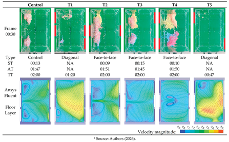
One aspect that distinguishes the Control configuration from the other treatments is the completely heterogeneous distribution of the polystyrene spheres. All face-to-face treatments — T2, T3, and T4 — exhibit at least some areas containing spheres of the same color. One expected outcome of the experiment is that a lower degree of color mixing corresponds to reduced interaction between air masses and, consequently, less turbulent ventilation. Introducing any obstacle (treatment) into the sample immediately generates some degree of airflow separation, which explains why the treatments maintain at least partial separation in the test area, a behavior not observed in the Sample Control. Among the face-to-face treatments, T3 exhibits the greatest behavioral similarity to the Sample Control. Both have the same number of inlet windows and produce very similar airflow patterns. However, T3 presents dead zones, as do the other treatments (T2 and T4), leading to the inference that in face-to-face treatments, closed windows consistently generate dead zones near the corners of the parallel walls (Table 3).
If the obstacles represent the treatments and, based on the behavior of the Control sample in which no obstacles are present and therefore no treatments are applied, observational inferences were made about the interaction of air masses inside the prototype, considering the window positions. The first observation is the significant efficiency of the diagonal treatments T1 and T5 compared with the other tests since they did not exhibit areas of material deposition at the end of the two-minute experiment. When comparing this result with the performance of the Control, and while acknowledging the inherent qualitative uncertainties of the experiment, it can be stated that the diagonal positioning of the openings influences the acceleration of indoor airflow more strongly than the number of openings. In these diagonal treatments, there is control over both the amount of incoming and outgoing airflow and the length of the airflow path inside the prototype, with far fewer interactions between opposing air masses. This makes cross ventilation more laminar and less turbulent. This helps explain why T2 and T5 have the same number of inlet and outlet openings, yet T5 is considerably more efficient.
Between the diagonal treatments T1 and T5, treatment T5 is even more efficient, especially considering the shorter time, 38 seconds, required to clean the prototype. This suggests that an optimal point exists between the middle and the end of the parallel façades that allows the creation of ideal diagonal and opposing openings. Such openings can balance the incoming and outgoing airflow to achieve maximum efficiency in terms of indoor airspeed, at least for this rectangular geometry and scale.
Focusing on treatment T5 and advancing its comparative modeling in Ansys Fluent and based on the calibration demonstrated between the empirical and numerical models, it was possible to draw inferences about the causal mechanisms explaining why treatment T5 exhibits the highest efficiency in terms of particle velocity. Using two cameras, one positioned above the prototype and another at its side, the movement of the particles was observed during the 38 seconds preceding the complete clearing of the model. In the frames at 5, 15, and 30 seconds, it was noted that the polystyrene particles initially moved toward the corner of the prototype at 5 seconds. Upon encountering the accumulation of beads, they entered suspension and interacted with the diagonal airflow between the open windows. This motion triggered the formation of vertical vortices, which kept the particles suspended above the floor of the prototype, directing them into a continuous exhaust flow and leading to their expulsion from the model. These frames are presented in Figure 14.
The computational CFD simulations of the five treatments plus the control were previously presented in Bittar (2025). For the present analysis, we examined the nuances of treatment T5 in greater depth within the CFD environment, discretizing the simulation model into smaller sections. Although the simulation outputs represent an average snapshot of the wind behavior across the prototype, they provide valuable insight into the dynamics of mean vortex structures. Treatment T5 distinguishes itself from the other configurations not only by exhibiting stronger airflow patterns but also by the predominance of nearly exclusive vertical vortices. These vertical vortices effectively suppress the formation of horizontal vortices, which are typically responsible for generating deposition regions that correspond to dead zones.
Between 5 and 10 seconds, when it is still possible to identify a clear separation of colors corresponding to the horizontal vortices, the particles have not yet reached a suspended state. When the first particles become suspended at around 15 seconds, the vertical motions begin to mix with the horizontal ones, forming a kind of twisting pattern that combines both vortex structures. By 30 seconds, nearly all particles move according to this combined pattern, accelerating toward the diagonal outlet. The longer path between the inlet and outlet in the diagonal treatments also means that the particle gains more speed before colliding with any wall and consequently emerges from this interaction still with significant velocity.
Exploring this reasoning within the CFD simulations, we concluded that, for the sample analyzed and considering the experimental uncertainties, without any intention of generalization, the diagonal treatments tend to produce, on average, 35 percent higher airflow velocities when they have the same number of openings, solely due to their positions. This notion becomes evident when we compare the mean layers of treatments T2 and T5, which contain the same number of openings but differ only in their placement, in the same proportion in which we observe a more intense action of the vertical vortices in the diagonal treatment (Figure 15).
Seeking to understand how the horizontal vortices manifest and lose definition in the diagonal treatments, we analyzed the initial frames starting at 5 seconds: 5, 7, 9, 11, and 13 seconds, which correspond to moments in which changes can be observed in the distribution of areas with clearly separated colors. In the first 5 seconds, the colored regions remain practically the same, although more concentrated in just over 70 percent of the area they initially occupied. Two seconds later, at 7 seconds, this region becomes even more concentrated, occupying about 55 percent of the original area, and the separation of the four colors is still visible. However, the magenta polystyrene beads begin to occupy a significantly smaller region, becoming more concentrated. At 9 seconds, the magenta beads are already completely mixed with the yellow beads, and part of the latter begins to exchange positions with the former, a typical characteristic of a horizontal vortex. At this moment, the orange beads begin to be expelled from the model, while the blue region becomes more elongated along the prototype wall. In the next frame, at 11 seconds, the yellow region becomes less elongated and more compact, indicating the location where the single small horizontal vortex visible in this treatment is formed. This sequence of events is presented in Figure 16.
The empirically observed flow patterns at the floor layer of the prototype are in close agreement with those obtained through CFD simulation of the same layer. Therefore, it can be stated that, despite the experimental uncertainties associated with the polystyrene beads, particularly their self-weight and the magnetic interaction between them, the analog method for visualizing wind effects proves to be a useful and efficient approach for understanding ventilation behavior in buildings subjected to low-velocity airflow, such as the 5 m/s condition adopted in this study. Although not evaluated here, it is expected that the proposed technique may also be effective under conditions of more intense ventilation, potentially serving as an alternative to conventional methods such as colored smoke. In this regard, the technique offers advantages related to simplicity, ease of handling, and significantly lower cost. Additional investigations under different geometric configurations and airflow velocities may be carried out in future studies, which could further consolidate the use of polystyrene beads as an effective alternative for visualizing wind effects in a broader range of applications.
7. Conclusion
The main experimental uncertainties between the physical prototype and the computational simulation are related to the weight of the Styrofoam balls. Although very light, they tend to accumulate in certain positions. Additionally, friction between them during the experiment leads to the phenomenon of electromagnetic static charge, which may exert some unmeasured influence on the results. The computer simulation, in contrast, represents an average of the airflow movements in discrete planes, functioning as a static snapshot of the average ventilation behavior under steady flow conditions. Considering these scientific simplifications and analyzing the two strategies in a complementary manner, we concluded that the diagonal positioning of openings substantially accelerates wind speed in indoor environments. This design strategy is more effective than simply increasing the number of openings when the intention is to enhance airspeed and air renewal. In a similar sense, the movement of particles can be compared to people in a crowd attempting to enter an indoor environment. When many entry points are available, the crowd progresses at a slower pace. Conversely, a smaller number of openings positioned diagonally creates a longer and narrower path, allowing greater acceleration and consequently higher speeds.
8. Patents
This section is not mandatory but may be added if there are patents resulting from the work reported in this manuscript.
Supplementary Materials
The following supporting information can be downloaded at the website of this paper posted on Preprints.org, Video S1: Experimental setup and flow visualization.
Author Contributions
Conceptualization, Odenir de Almeida and André Araujo; methodology, Odenir de Almeida; software, Mariana Bittar and Odenir de Almeida; validation, Odenir de Almeida and Mariana Bittar; formal analysis, Themis Martins; investigation, Themis Martins; resources, André Araujo; data curation, André Araujo; writing; original draft preparation, Odenir de Almeida and André Araujo; writing; review and editing, André Araujo and Themis Martins; visualization, Odenir de Almeida; supervision, André Araujo; project administration, André Araujo; funding acquisition, André Araujo. All authors have read and agreed to the published version of the manuscript.
Funding
This research was funded by the Minas Gerais Research Foundation (FAPEMIG), grant number APQ-01926-17.
Institutional Review Board Statement
Not applicable.
Informed Consent Statement
Not applicable.
Data Availability Statement
The data presented in this study are available from the corresponding author upon reasonable request.
Acknowledgments
The authors would like to acknowledge the financial support provided by the Minas Gerais Research Foundation (FAPEMIG) under grant number APQ-01926-17. The authors also acknowledge the institutional support of the Federal University of Uberlândia, as well as the infrastructure and technical support provided by the Triangle BIM Hub and the CPAERO (Center for Experimental Aerodynamics). During the preparation of this manuscript, the authors used ChatGPT (OpenAI, version January 2026) exclusively for grammatical revision and precise translation of technical terms. The authors reviewed and edited the output and take full responsibility for the content of this publication.
Conflicts of Interest
The authors declare no conflicts of interest.
Abbreviations
The following abbreviations are used in this manuscript:
| CFD | Computational Fluid Dynamics |
References
- Kolarevic, B.; Malkawi, A.M. Performative Architecture: Beyond Instrumentality; Spon Press: New York, 2004; ISBN 978-0415700832. [Google Scholar]
- Sutherland, I. Sketchpad: A Man–Machine Graphical Communication System; Massachusetts Institute of Technology (MIT), 1963. [Google Scholar]
- Eastman, C. The Use of Computers Instead of Drawings in Building Design. J. Am. Inst. Archit. 1975, 63, 46–50. [Google Scholar]
- Batty, M. Cities and Complexity: Understanding Cities with Cellular Automata, Agent-Based Models, and Fractals; MIT Press: Boston, 2007; ISBN 9780262524797. [Google Scholar]
- Hensen, J.L.M.; Lamberts, R. Introduction to Building Performance Simulation. In Building Performance Simulation for Design and Operation; Spon Press: Oxon, 2014; pp. 1–14. [Google Scholar]
- Olgyay, V. Design with Climate: Bioclimatic Approach to Architectural Regionalism; University Press: Princeton, New Jersey, 2015; ISBN 9780691169736. [Google Scholar]
- Givoni, B. Basic Study of Ventilation Problems in Housing in Hot Countries; Building Research Station, Technion, Israel Institute of Technology: Haifa, 1962. [Google Scholar]
- Givoni, B. Climate Considerations in Building and Urban Design; John Wiley & Sons: London, 1998; ISBN 978-0-471-29177-0. [Google Scholar]
- Engineers, C.C.I. of B.S. Natural Ventilation in Non-Domestic Buildings; Chartered Institution of Building Services Engineers: London, 2005; ISSN 1903287561.
- ANSI/ASHRAE Standard 62.1-2019; Ventilation for Acceptable Indoor Air Quality. 2019.
- Cheng, C.K.C.; Dai, Z.; Liu, C.H. Wind Induced Natural Ventilation of Re Entrant Bays in a High Rise Building. J. Wind Eng. Ind. Aerodyn. 2010, 98, 853–859. [Google Scholar] [CrossRef]
- Cui, P.Y.; Li, X.; Liu, C.H. Effects of Wind and Buoyancy Interaction on Single Sided Natural Ventilation in Buildings. J. Wind Eng. Ind. Aerodyn. 2017, 171, 380–394. [Google Scholar] [CrossRef]
- Tan, L.; Yuan, Y. Computational Fluid Dynamics Simulation and Performance Optimization of an Electrical Vehicle Air-Conditioning System. Alexandria Eng. J. 2022, 61, 315–328. [Google Scholar] [CrossRef]
- Irwin, P.; Denoon, R.; Scott, D. Wind Tunnel Testing of High-Rise Buildings; Routledge: London, 2013; ISBN 9780415714594. [Google Scholar]
- Cuce, E.; Sher, F.; Sadiq, H.; Cuce, P.M.; Guclu, T.; Besir, A.B. Sustainable Ventilation Strategies in Buildings: CFD Research. Sustain. Energy Technol. Assessments 2019, 36, 100540. [Google Scholar] [CrossRef]
- Karava, P.; Stathopoulos, T.; Athienitis, A.K. Wind Driven Cross Ventilation of Buildings with Large Openings. J. Wind Eng. Ind. Aerodyn. 2007, 95, 943–966. [Google Scholar] [CrossRef]
- Zheng, X.; Shi, Z.; Xuan, Z.; Qian, H. Natural Ventilation. Handbook of Energy Systems in Green Buildings 2018, 1227–1270. [Google Scholar]
- Kabošová, L. Analysis of Wind-Adaptive Architecture. In Proceedings of the IOP Conference Series: Materials Science and Engineering 2020, Vol. 867, 12014. [Google Scholar] [CrossRef]
- Abbas, G.M.; Dino, İ.G. A Parametric Design Method for CFD-Supported Wind-Driven Ventilation. In Proceedings of the IOP Conference Series: Materials Science and Engineering 2019, Vol. 609, 32010. [Google Scholar] [CrossRef]
- Poh, H.J.; Chiu, P.H.; Nguyen, H.; Xu, G.; Chong, C.S.; Lee, L.T.; Po, K.; Ping, T.P.; Wong, N.; Li, R.; et al. Airflow Modelling Software Development for Natural Ventilation Design - Green Building Environment Simulation Technology. In Proceedings of the IOP Conference Series: Earth and Environmental Science 2019, Vol. 238, 12077. [Google Scholar] [CrossRef]
- Kwok, H.; Cheng, J.; Li, A.; Tong, J.; Lau, A. Impact of Shaft Design to Thermal Comfort and Indoor Air Quality of Floors Using BIM Technology. J. Build. Eng. 2022, 51, 104326. [Google Scholar] [CrossRef]
- Obeidat, B.; Kamal, H.; Almalkawi, A. CFD Analysis of an Innovative Wind Tower Design with Wind-Inducing Natural Ventilation Technique for Arid Climatic Conditions. J. Ecol. Eng. 2021, 22, 86–97. [Google Scholar] [CrossRef] [PubMed]
- Weerasuriya, A.U.; Zhang, X.; Gan, V.J.L.; Tan, Y. A Holistic Framework to Utilize Natural Ventilation to Optimize Energy Performance of Residential High-Rise Buildings. Build. Environ. 2019, 153, 218–232. [Google Scholar] [CrossRef]
- Li, W.; Subiantoro, A.; McClew, I.; Sharma, R.N. CFD Simulation of Wind and Thermal-Induced Ventilation Flow of a Roof Cavity. Build. Simul. 2022, 15, 1611–1627. [Google Scholar] [CrossRef]
- Laurini, E.; De Vita, M.; De Berardinis, P.; Friedman, A. Passive Ventilation for Indoor Comfort: A Comparison of Results from Monitoring and Simulation for a Historical Building in a Temperate Climate. Sustainability 2018, 10, 1565. [Google Scholar] [CrossRef]
- Khosrowjerdi, S.; Sarkardeh, H.; Kioumarsi, M. Effect of Wind Load on Different Heritage Dome Buildings. Eur. Phys. J. Plus 2021, 136, 2133. [Google Scholar] [CrossRef]
- Izadyar, N.; Miller, W.; Rismanchi, B.; Garcia-Hansen, V.; Matour, S. Balcony Design and Surrounding Constructions Effects on Natural Ventilation Performance and Thermal Comfort Using CFD Simulation: A Case Study. J. Build. Perform. Simul. 2023, 16, 537–556. [Google Scholar] [CrossRef]
- Jingyuan, S.; Changkai, Z.; Yanan, L. CFD Analysis of Building Cross-Ventilation with Different Angled Gable Roofs and Opening Locations. Buildings 2023, 13, 2716 . [Google Scholar] [CrossRef]
- Hawendi, S.; Gao, S. Impact of an External Boundary Wall on Indoor Flow Field and Natural Cross-Ventilation in an Isolated Family House Using Numerical Simulations. J. Build. Eng. 2017, 10, 109–123. [Google Scholar] [CrossRef]
- Elwan, M.; Dewair, H.A. Lattice Windows as a Natural Ventilation Strategy in Hot, Humid Regions. In Proceedings of the IOP Conference Series: Earth and Environmental Science (Simulation for a Sustainable Built Environment) 2019, Vol. 397, 12022. [Google Scholar]
- Yin, H.; Li, Y.; Zhang, D.; Han, Y.; Wang, J.; Zhang, Y.; Li, A. Airflow Pattern and Performance of Attached Ventilation for Two Types of Tiny Spaces. Build. Simul. 2022, 15, 1491–1506. [Google Scholar] [CrossRef]
- Lezcano, R.; Burgos, M.J. Airflow Analysis of the Haida Plank House, a Breathing Envelope. Energies 2021, 14, 4871. [Google Scholar] [CrossRef]
- Rocha, L.A.; Gomez, R.S.; Delgado, J.M.P.Q.; Vieira, A.N.O.; Santos, I.B.; Luiz, M.R.; Oliveira, V.A.B.; Oliveira Neto, G.L.; Vasconcelos, D.B.T.; Silva, M.J.V.; et al. Natural Ventilation in Low-Cost Housing: An Evaluation by CFD. Buildings 2023, 13. [Google Scholar] [CrossRef]
- Kwok, H.L.; Cheng, J.C.P.; Li, A.T.Y.; Tong, J.C.K.; Lau, A.K.H. Multi-Zone Indoor CFD under Limited Information: An Approach Coupling Solar Analysis and BIM for Improved Accuracy. J. Clean. Prod. 2020, 244, 118912. [Google Scholar] [CrossRef]
- Nasrollahi, N.; Ghobadi, P. Field Measurement and Numerical Investigation of Natural Cross-Ventilation in High-Rise Buildings; Thermal Comfort Analysis. Appl. Therm. Eng. 2022, 211, 118500. [Google Scholar] [CrossRef]
- Fu, X.; Han, M. Analysis of Natural Ventilation Performance Gap between Design Stage and Actual Operation of Office Buildings. In Proceedings of the E3S Web of Conferences 2020, Vol. 172, 9110. [Google Scholar] [CrossRef]
- Elshafei, G.; Negm, A.; Bady, M.; Suzuki, M.; Ibrahim, M.G. Numerical and Experimental Investigations of the Impacts of Window Parameters on Indoor Natural Ventilation in a Residential Building. Energy Build. 2017, 141, 321–332. [Google Scholar] [CrossRef]
- Subhashini, S.; Thirumaran, K. CFD Simulations for Examining Natural Ventilation in the Learning Spaces of an Educational Building with Courtyards in Madurai. Build. Serv. Eng. Res. Technol. 2019, 41, 466–479. [Google Scholar] [CrossRef]
- Zhang, Z.; Yin, W.; Wang, T.; O’Donovan, A. Effect of Cross-Ventilation Channel in Classrooms with Interior Corridor Estimated by Computational Fluid Dynamics. Indoor Built Environ. 2022, 31, 1047–1065. [Google Scholar] [CrossRef]
- D’Alicandro, A.C.; Mauro, A. Effects of Operating Room Layout and Ventilation System on Ultrafine Particle Transport and Deposition. Atmos. Environ. 2022, 270, 118901. [Google Scholar] [CrossRef]
- Dao, H.T.; Kim, K. Behavior of Cough Droplets Emitted from Covid-19 Patient in Hospital Isolation Room with Different Ventilation Configurations. Build. Environ. 2022, 209, 108649. [Google Scholar] [CrossRef] [PubMed]
- Zhang, T.; Zhang, Y.; Li, A.; Gao, Y.; Rao, Y.; Zhao, Q. Study on the Kinetic Characteristics of Indoor Air Pollutants Removal by Ventilation. Build. Environ. 2022, 207, 108535. [Google Scholar] [CrossRef]
- Bovo, M.; Santolini, E.; Barbaresi, A.; Tassinari, P.; Torreggiani, D. Assessment of Geometrical and Seasonal Effects on the Natural Ventilation of a Pig Barn Using CFD Simulations. Comput. Electron. Agric. 2022, 193, 106652. [Google Scholar] [CrossRef]
- Küçüktopcu, E.; Cemek, B.; Simsek, H.; Ni, J. Computational Fluid Dynamics Modeling of a Broiler House Microclimate in Summer and Winter. Animals 2022, 12, 867. [Google Scholar] [CrossRef]
- Zhang, Y.; Kacira, M. Analysis of Climate Uniformity in Indoor Plant Factory System with Computational Fluid Dynamics (CFD). Biosyst. Eng. 2022, 220, 73–86. [Google Scholar] [CrossRef]
- Lukiantchuki, M.A.; Shimomura, A.P.; Silva, F.M.; Caram, R.M. Wind Tunnel and CFD Analysis of Wind-Induced Natural Ventilation in Sheds Roof Building: Impact of Alignment and Distance between Sheds. Int. J. Vent. 2020, 19, 141–162. [Google Scholar] [CrossRef]
- Cui, P.; Chen, W.; Wang, J.; Zhang, J.; Huang, Y.; Tao, W. Numerical Studies on Issues of Re-Independence for Indoor Airflow and Pollutant Dispersion within an Isolated Building. Build. Simul. 2022, 15, 1259–1276. [Google Scholar] [CrossRef]
- Mei, X.; Zeng, C.; Gong, G. Predicting Indoor Particle Dispersion under Dynamic Ventilation Modes with High-Order Markov Chain Model. Build. Simul. 2022, 15, 1243–1258. [Google Scholar] [CrossRef]
- Kumar, N.; Bardhan, R.; Kubota, T.; Tominaga, Y.; Shirzadi, M. Parametric Study on Vertical Void Configurations for Improving Ventilation Performance in the Mid-Rise Apartment Building. Build. Environ. 2022, 215, 108969. [Google Scholar] [CrossRef]
- Kong, X.; Chang, Y.; Li, N.; Li, H.; Li, W. Comparison Study of Thermal Comfort and Energy Saving under Eight Different Ventilation Modes for Space Heating. Build. Simul. 2022, 15, 1323–1337. [Google Scholar] [CrossRef]
- Zhang, X.; Weerasuriya, A.U.; Wang, J.; Li, C.Y.; Chen, Z.; Tse, K.T.; Hang, J. Cross-Ventilation of a Generic Building with Various Configurations of External and Internal Openings. Build. Environ. 2022, 207, 108447. [Google Scholar] [CrossRef]
- Sakiyama, N.R.M.; Frick, J.; Bejat, T.; Garrecht, H. Using CFD to Evaluate Natural Ventilation through a 3D Parametric Modeling Approach. Energies 2021, 14, 2197. [Google Scholar] [CrossRef]
- Donn, M.R.; Bakshi, N. A Natural Ventilation “Calculator”: The Challenge of Defining a Representative ‘Performance Sketch’ in Practice and Research. In Proceedings of the IOP Conference Series: Materials Science and Engineering 2019, Vol. 609, 72045. [Google Scholar] [CrossRef]
- Sakiyama, N.R.M.; Carlo, J.C.; Frick, J.; Garrecht, H. Perspectives of Naturally Ventilated Buildings: A Review. Renew. Sustain. Energy Rev. 2020, 130, 109933. [Google Scholar] [CrossRef]
- Almeida, O.; Pinto, W.J.G.S.S.; Rosa, C. Experimental Analysis of the Flow Over a Commercial Vehicle-Pickup. Int. Rev. Mech. Eng. 2007, 11, 530–537. [Google Scholar] [CrossRef]
- Almeida, O. The Development of an Experimental Aerodynamics Research Center in Brazil. Int. J. Adv. Eng. Res. Sci. 2021, 8, 16. [Google Scholar] [CrossRef]
- Alves, R.M.; Almeida, O. Validation of Experimental and Numerical Techniques for Flow Analysis over an Ahmed Body. Int. J. Eng. Res. Appl. 2017, 7, 63–71. [Google Scholar] [CrossRef]
- Nishioka, A.H.; de Almeida, O. Study, Design and Test of a LENZ-Type Wind Turbine. Int. J. Adv. Eng. Res. Sci. 2018, 5, 264–269. [Google Scholar] [CrossRef]
- Pinto, W.J.G.D.S. Numerical and Experimental Analysis of the Flow over a Commercial Vehicle–Pickup. Therm. Eng. 2018, 17, 92–102. [Google Scholar] [CrossRef]
- Jewel, B.B.; William, H.; Era, J.; Alan, P. Low-Speed Wind Tunnel Testing; Wiley India Pvt Ltd: India, 1999; Volume 3. [Google Scholar]
- Matsumoto, E.; Labaki, L.; Caram, R.M.; Kowaltowski, D.C.C.K. (ed. . A Aplicação de Ensaios Em Túnel de Vento No Processo de Projeto. In O processo de projeto em arquitetura: da teoria à tecnologia; Oficina de texto: São Paulo, SP, 2019.
- ANSYS FLUENT 22.0. Theory Guide; ANSYS Inc., 2022;
- Phillips, D.A.; Soligo, M.J. Will CFD Ever Replace Wind Tunnels for Building Wind Simulations? Int. J. High-Rise Build. 2019, 8, 107–116. [Google Scholar] [CrossRef]
- Cermak, J.E.; Poreh, M.; Peterka, J.A.; Ayad, S.S. Wind Tunnel Investigations of Natural Ventilation. J. Transp. Eng. 1984, 110, 67–79. [Google Scholar] [CrossRef]
- Blocken, B.; Carmeliet, J.; Stathopoulos, T. CFD Evaluation of Wind Speed Conditions in Passages between Parallel Buildings—Effect of Wall-Function Roughness Modifications for the Atmospheric Boundary Layer Flow. J. Wind Eng. Ind. Aerodyn. 2007, 95, 941–962. [Google Scholar] [CrossRef]
- Ouyang, K.; Haghighat, F. A Procedure for Calculating Thermal Response Factors of Multi-Layered Walls-State Space Method. Build. Environ. 1991, 26, 173–177. [Google Scholar] [CrossRef]
Figure 1.
The schematic view and dimensions of the building prototype model, expressed in millimeters.
Figure 1.
The schematic view and dimensions of the building prototype model, expressed in millimeters.
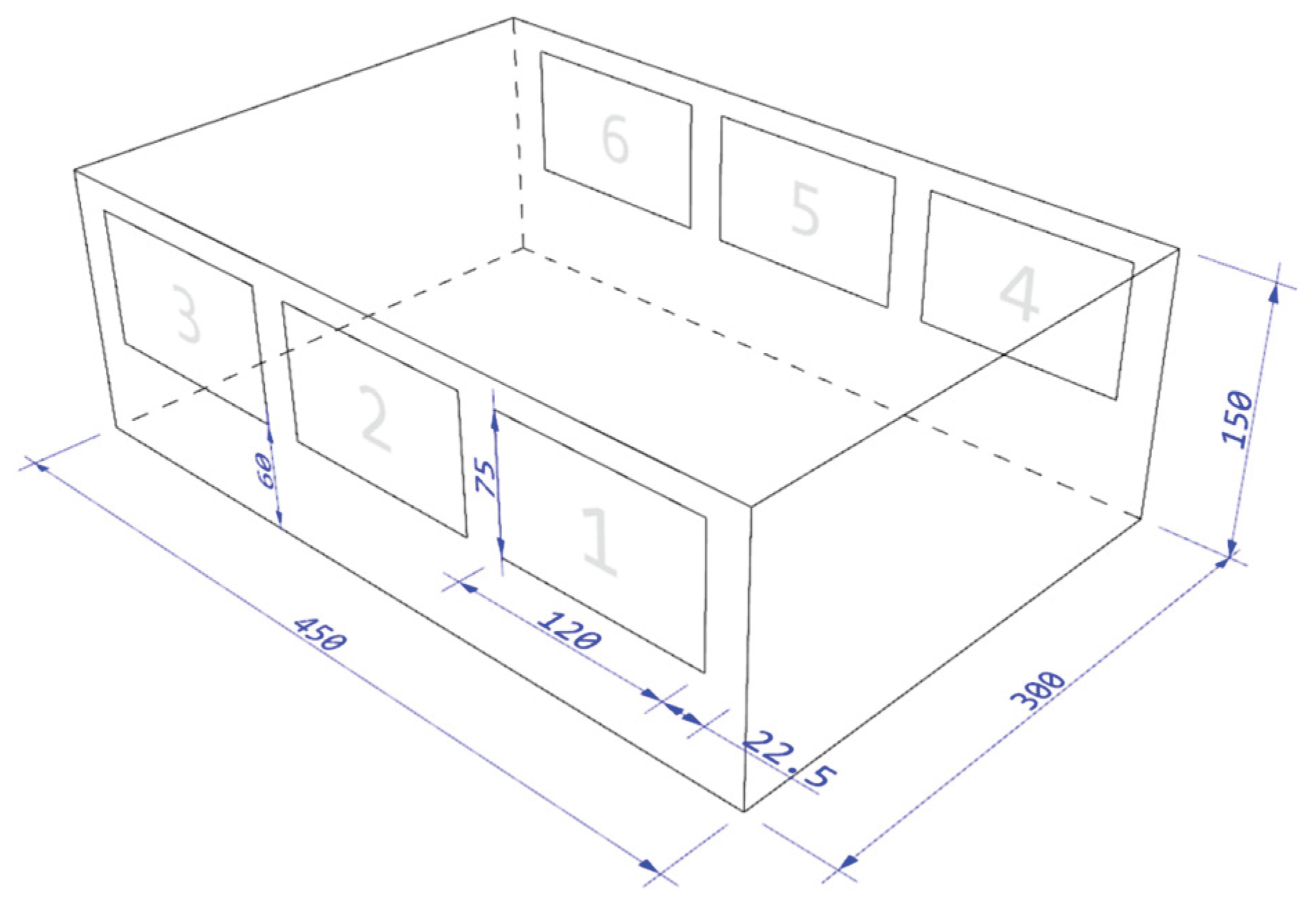
Figure 2.
WDN-CV model placed inside WT-test section.
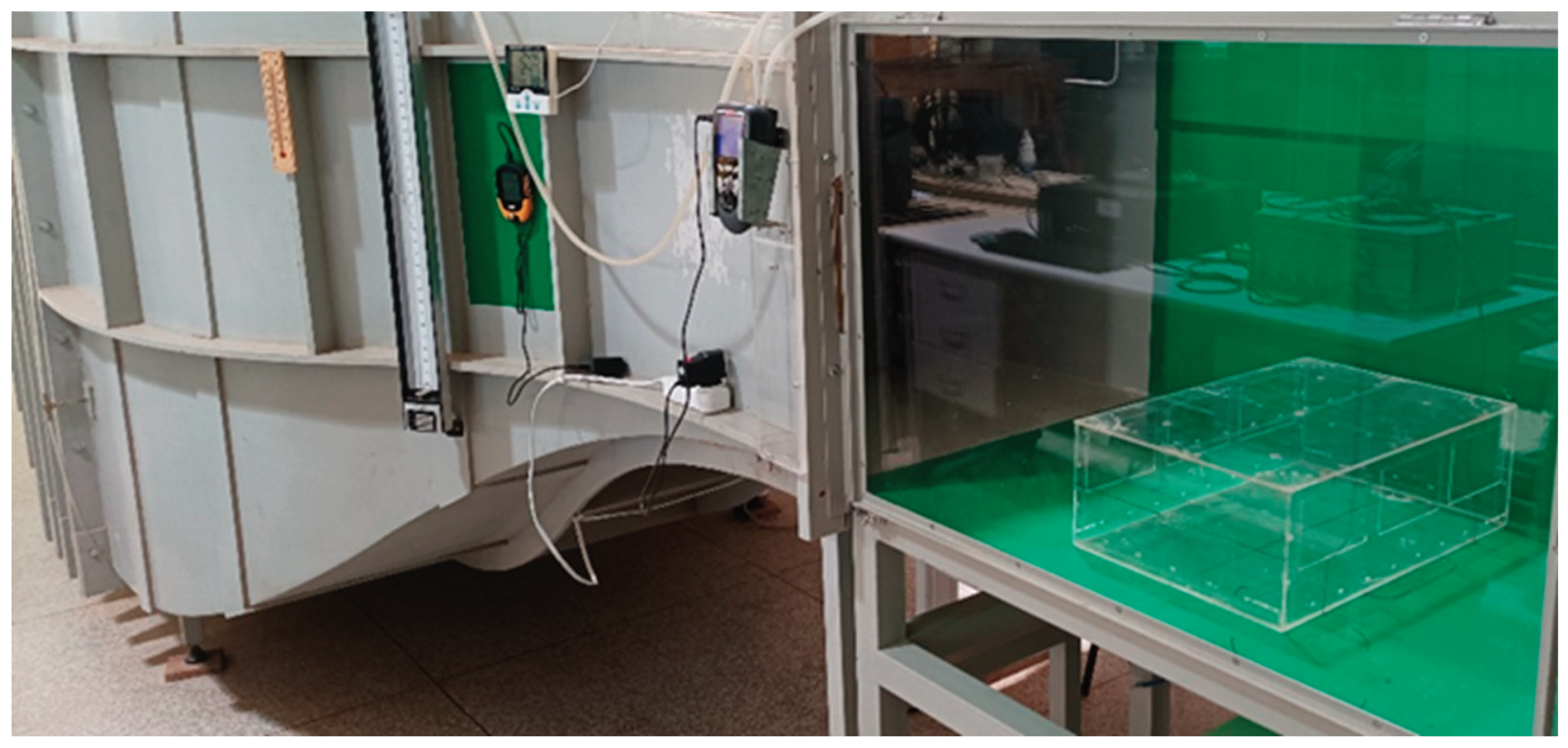
Figure 3.
Profiles of the mean wind speed and turbulence intensity in the wind tunnel.
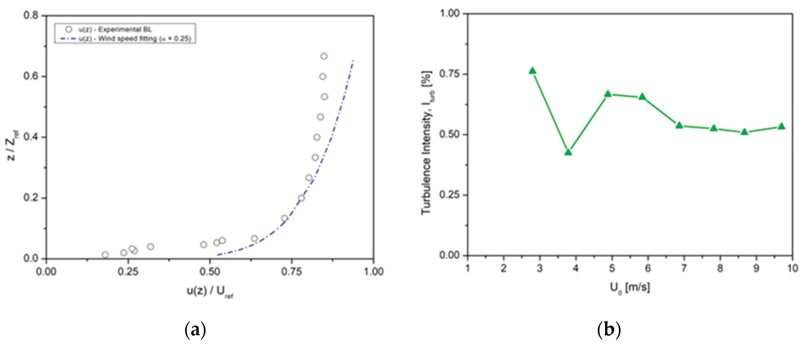
Figure 4.
Sample of statistically stationary data obtained in wind tunnel.
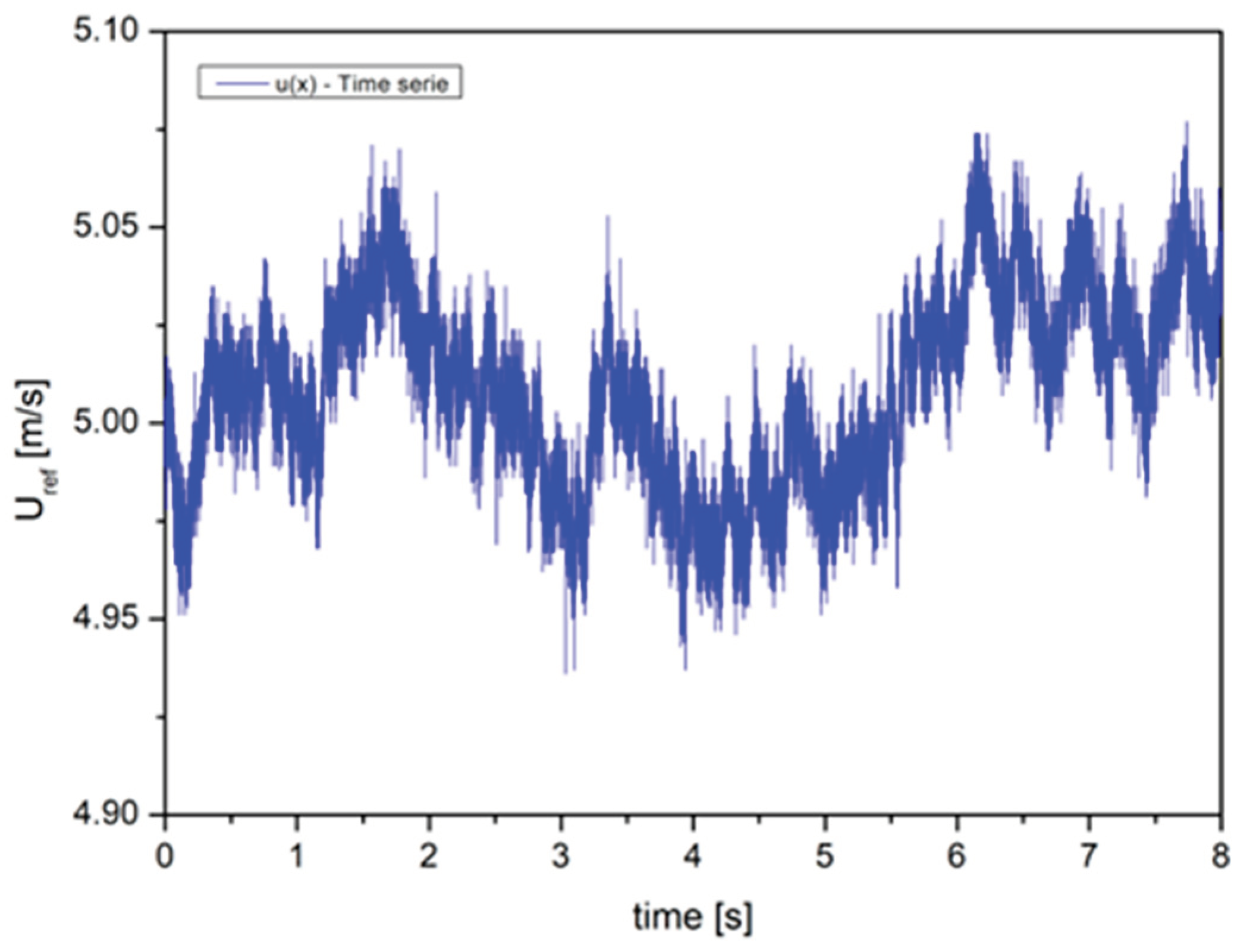
Figure 5.
u-velocity component measured over a horizontal line inside the building: (a) Schematic view; (b) Real probe positioning.
Figure 5.
u-velocity component measured over a horizontal line inside the building: (a) Schematic view; (b) Real probe positioning.
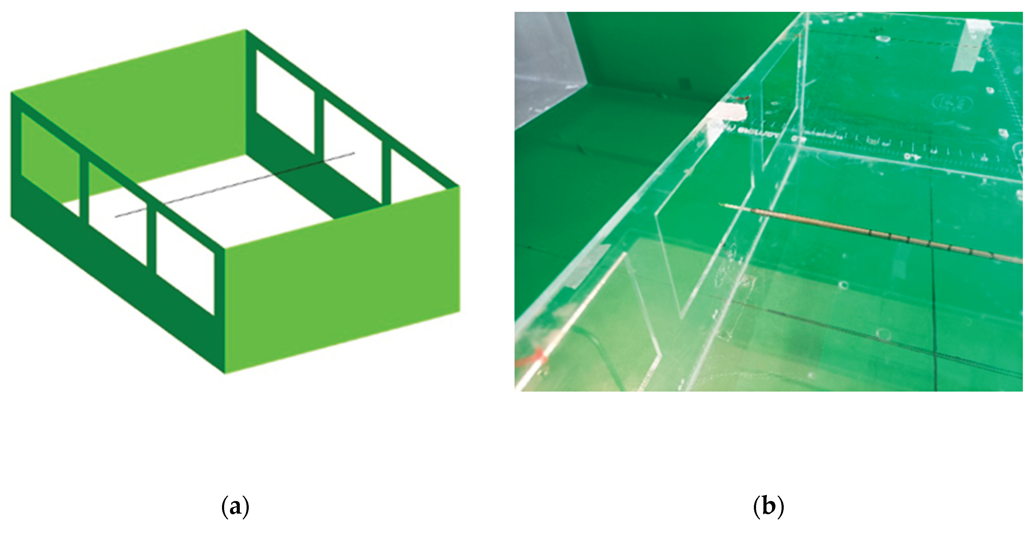
Figure 6.
u-velocity measured over the windows for Q (m3/s) calculation.
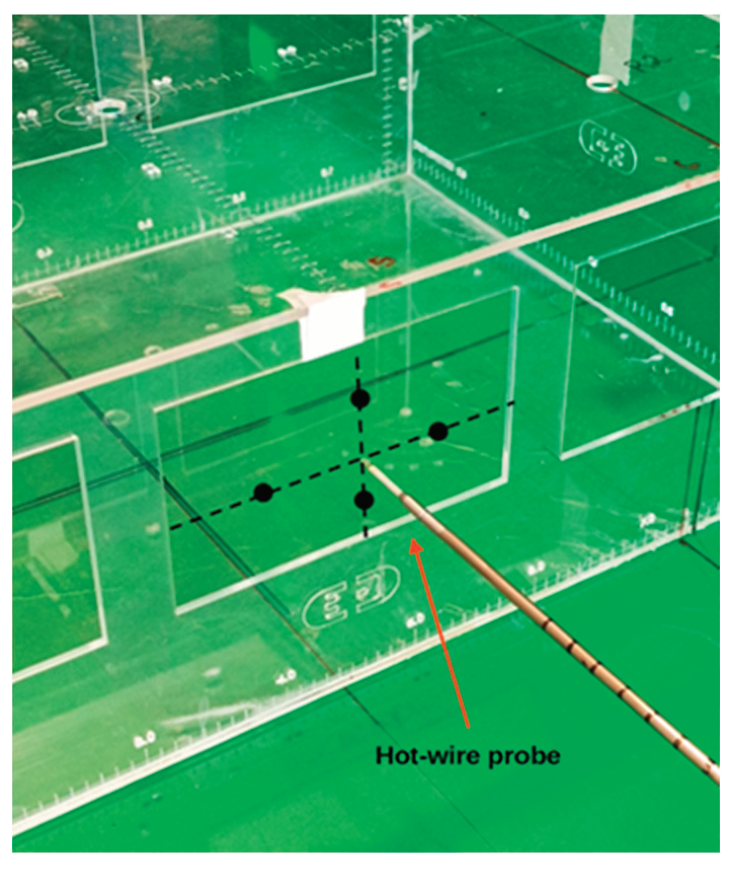
Figure 7.
Idealized tracer-based flow visualization technique using small polystyrene balls.
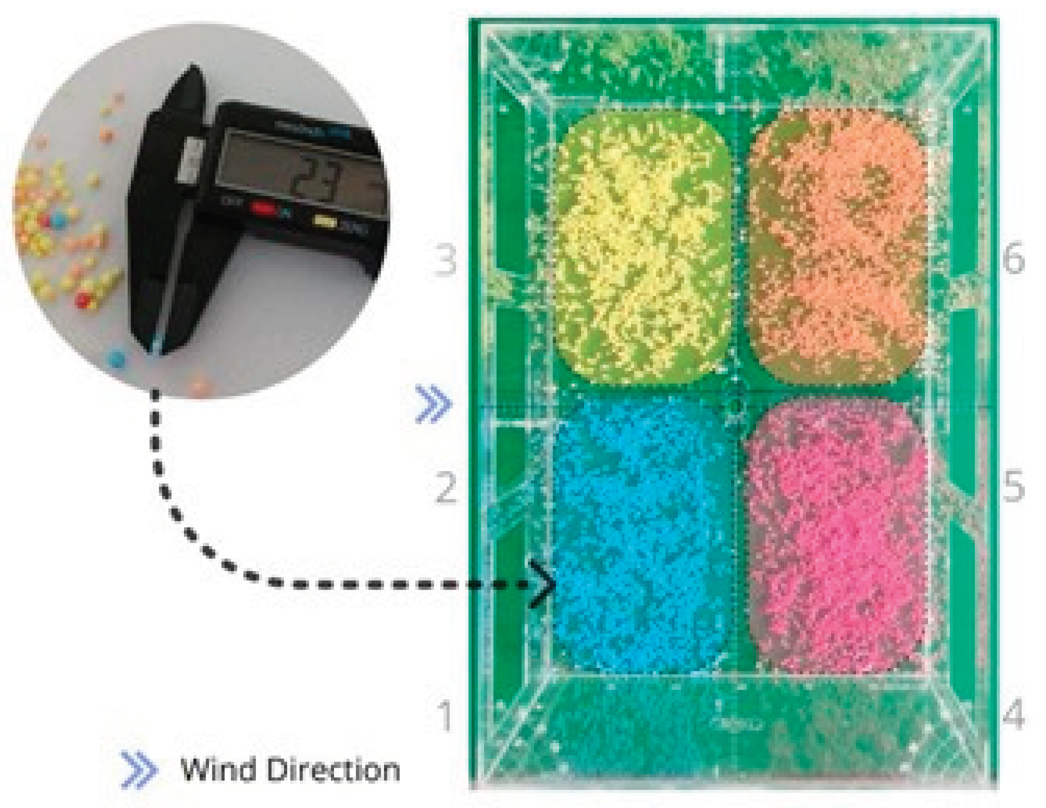
Figure 8.
Schematic view of the computational domain of the wind model.
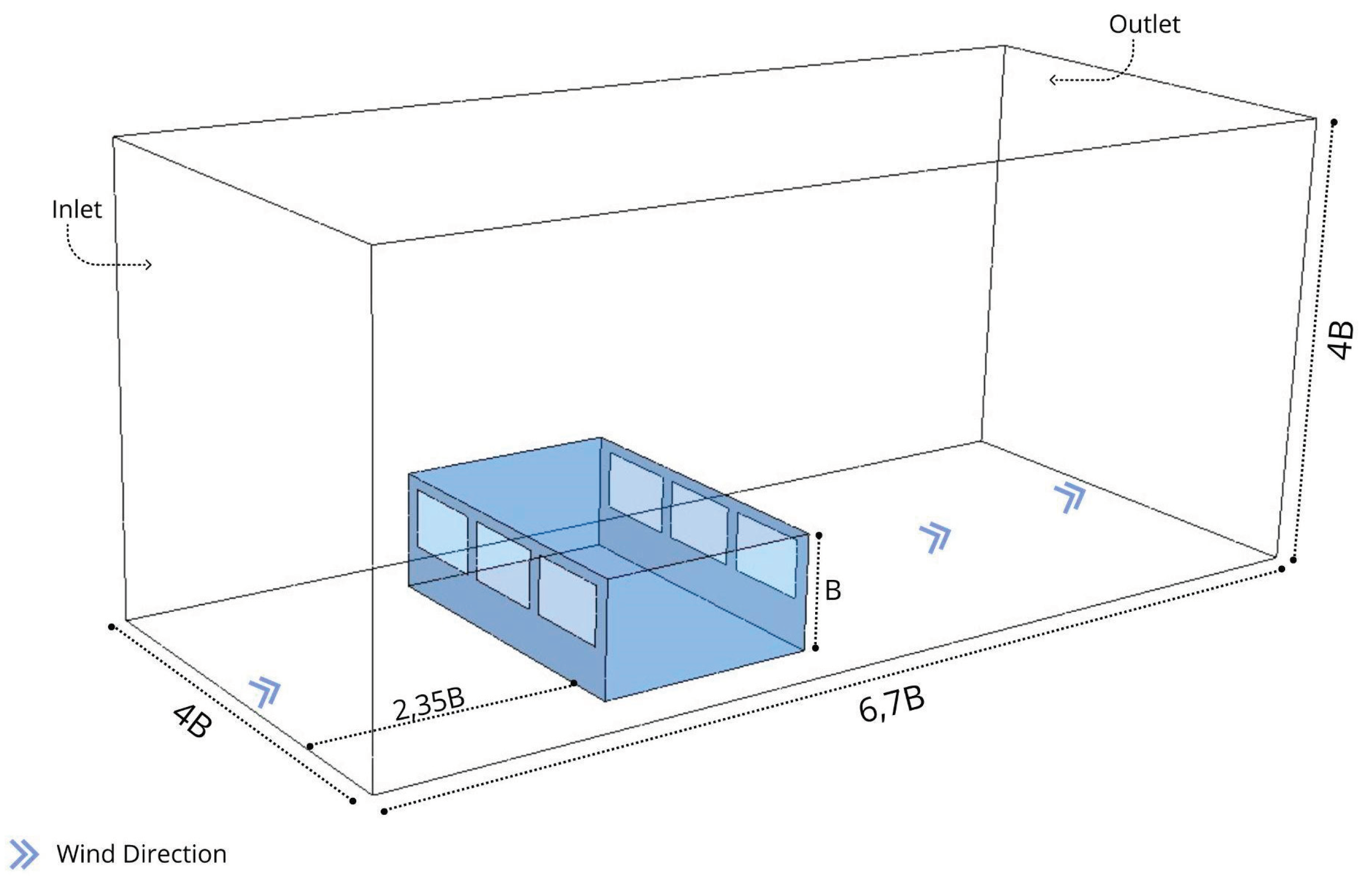
Figure 9.
Details of the mesh utilized in this research (mesh #4 with 2.7 × 10⁶ elements).
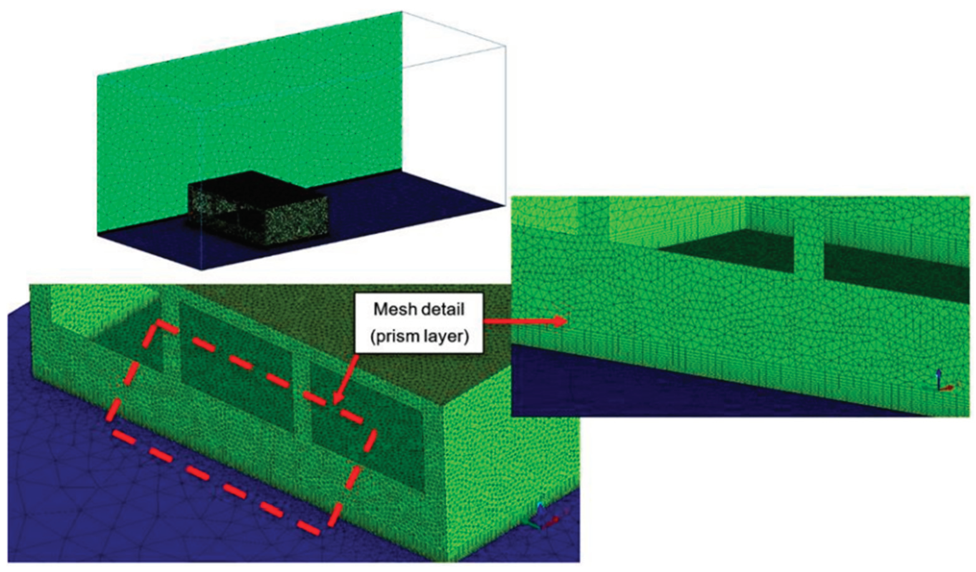
Figure 10.
(a) Volumetric flow rate through inlets for different grid distribution; (b) Indoor velocity distribution – windows 2 and 4 centerline.
Figure 10.
(a) Volumetric flow rate through inlets for different grid distribution; (b) Indoor velocity distribution – windows 2 and 4 centerline.
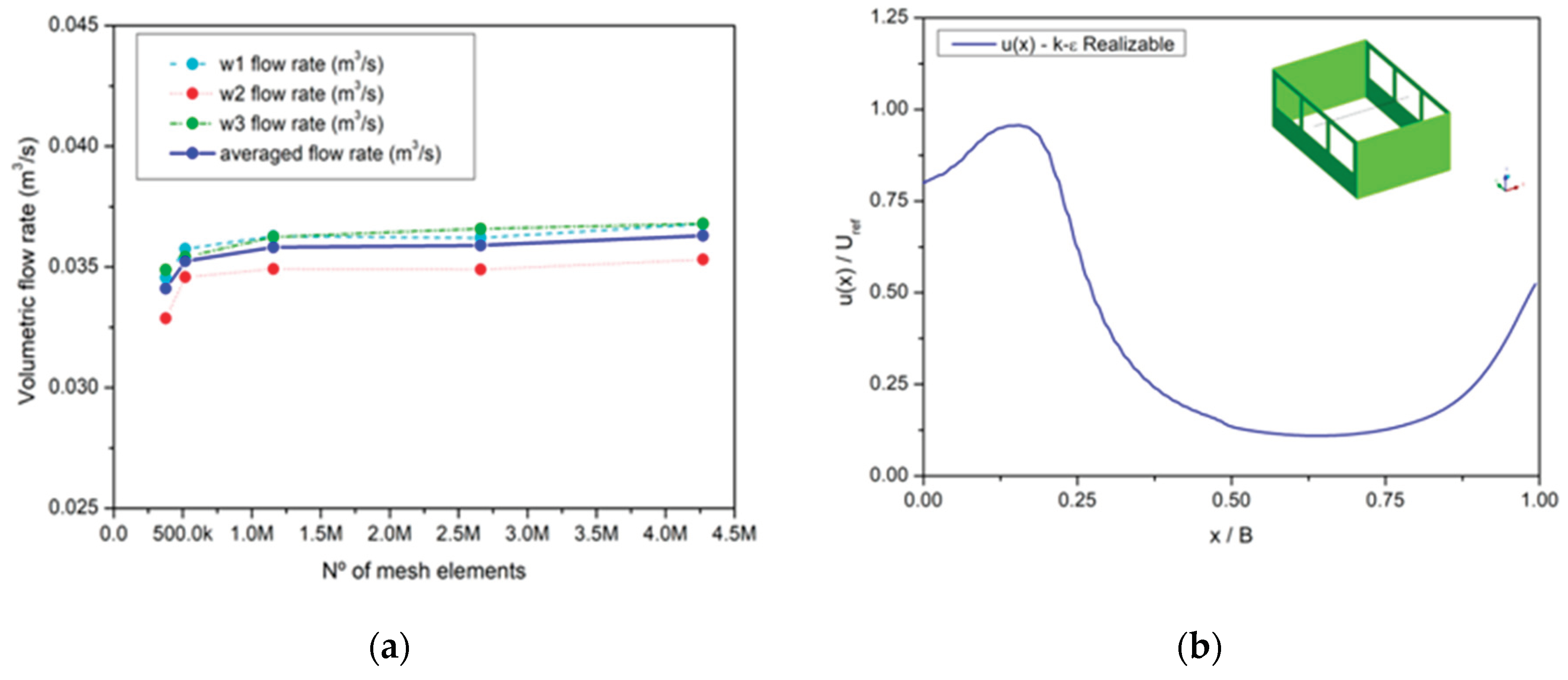
Figure 11.
Indoor velocity distribution between windows 2 and 4 for the control configuration with all windows open.
Figure 11.
Indoor velocity distribution between windows 2 and 4 for the control configuration with all windows open.
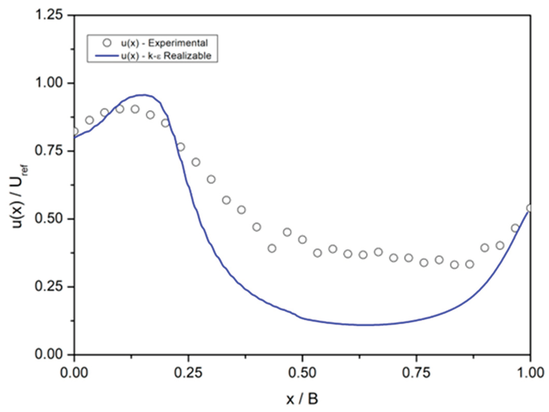
Figure 12.
Boundary layer development upstream the model building.
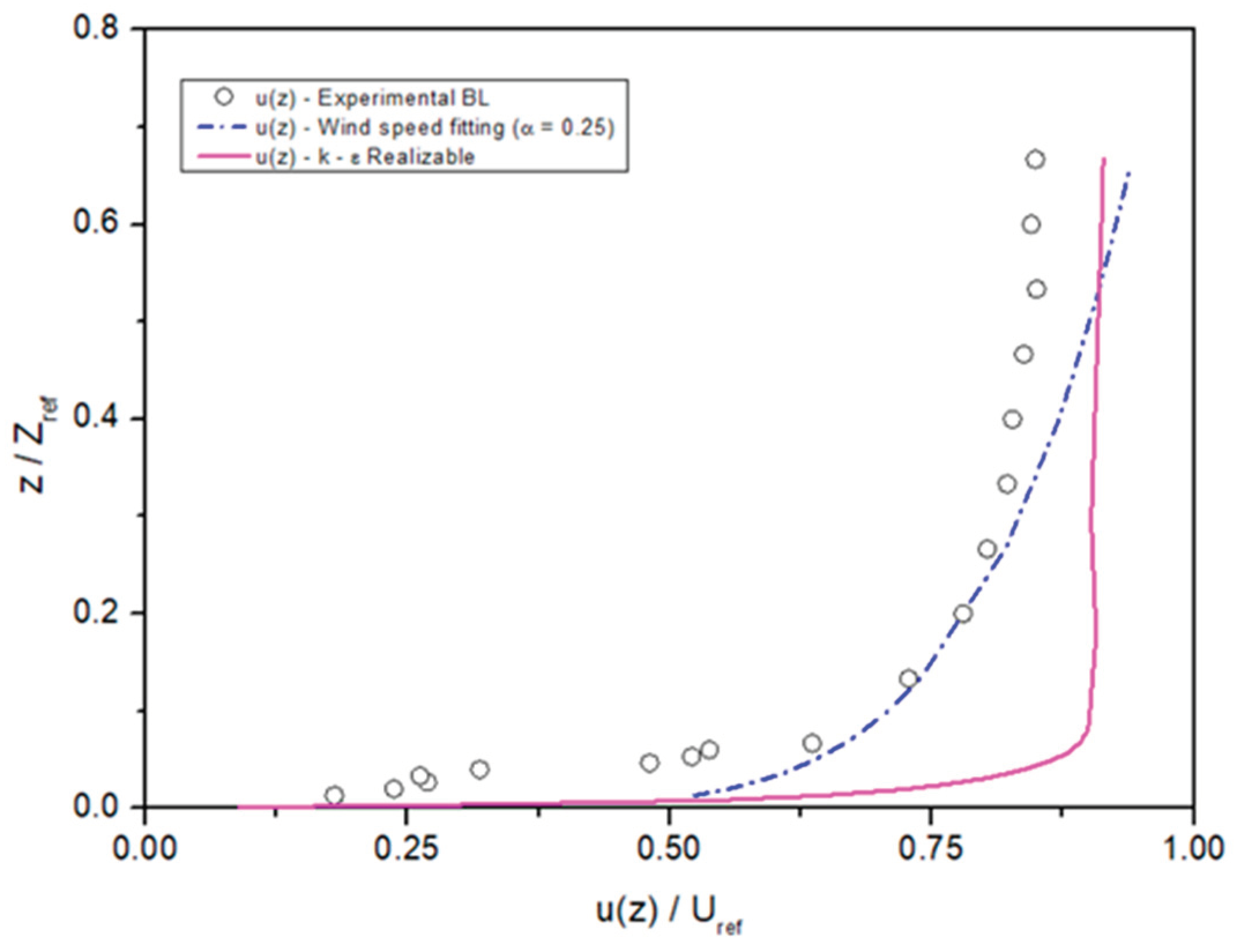
Figure 13.
Comparative possibilities between the experimental and numerical models under similar conditions with a wind source of 5 m/s in the Sample Control, with all six windows open: (a) Physical experiment at 0:00 (left) and 1 minute after the start of the experiment (right); (b) ANSYS Fluent simulation in horizontal planes: through the mid-height of the windows (left) and near the floor (right).
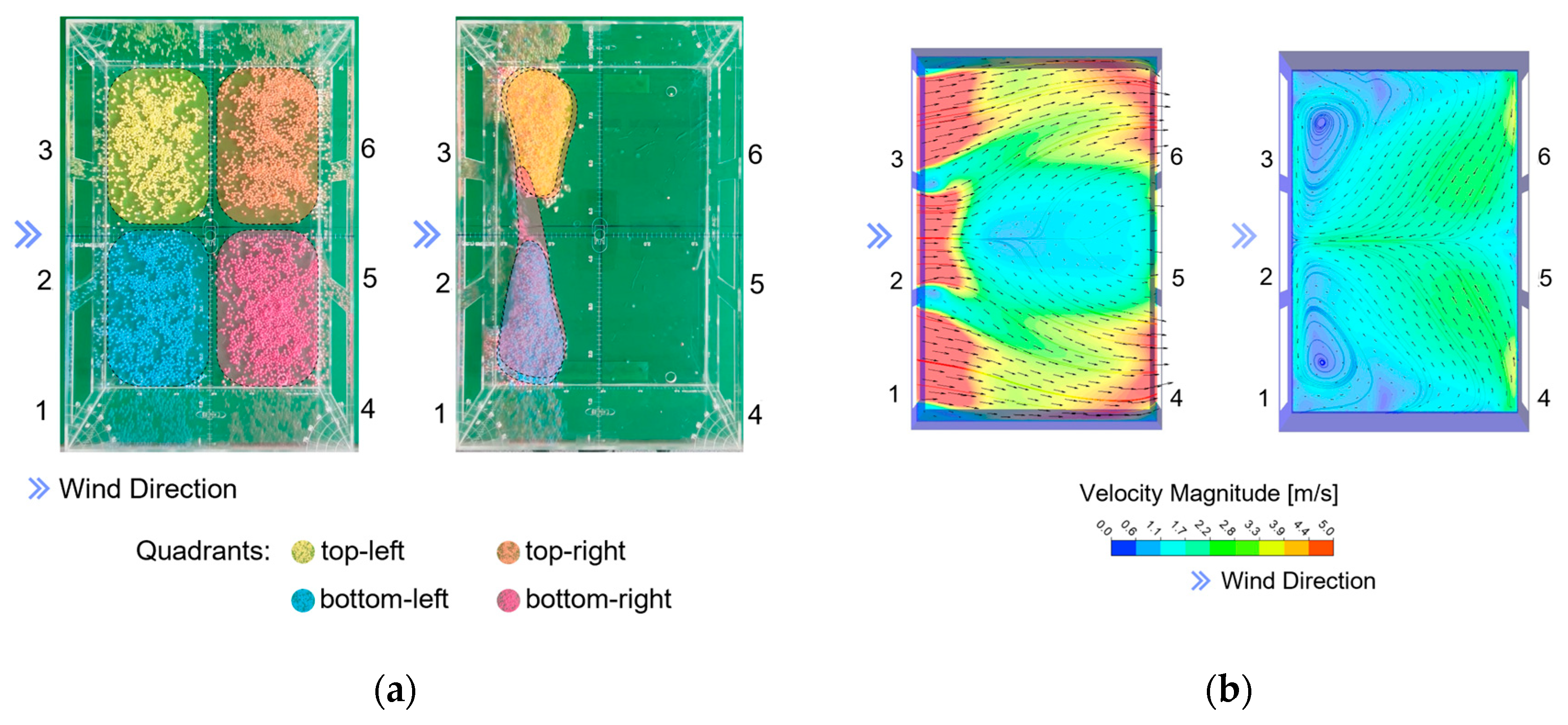
Figure 14.
Particle displacement in treatment T5 observed at 5, 15, and 30 seconds, recorded simultaneously by top and side cameras. The frames illustrate the formation of vertical vortices and the diagonal airflow interaction that promote the continuous suspension and expulsion of polystyrene particles inside the prototype.
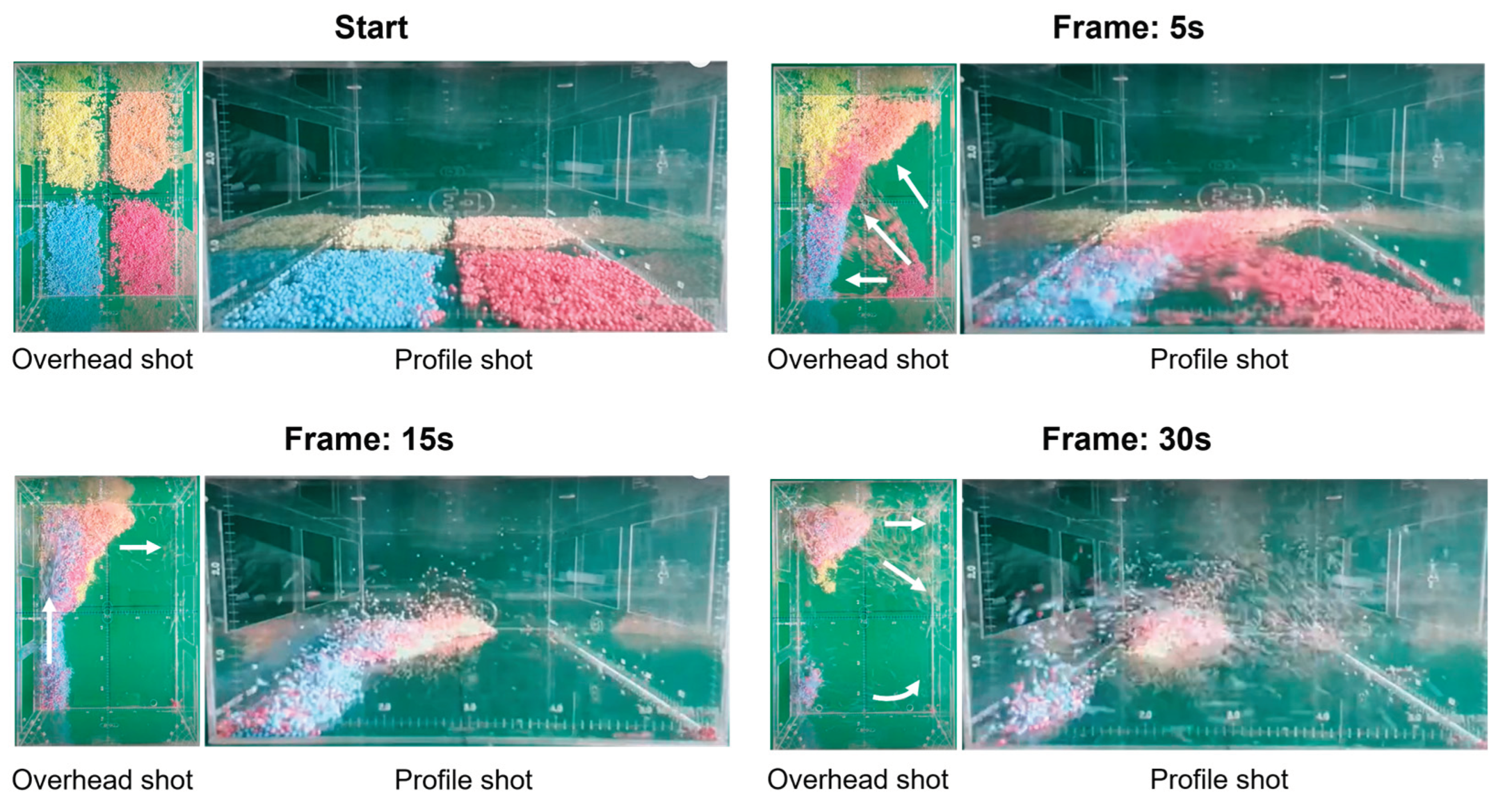
Figure 15.
Detailed analysis of the physical conditions in diagonal Treatment T5 through the numerical model: (a) floor layer projection, (b) perspective view of the middle layer, (c) perspective showing the flow velocities, and (d) section of the prototype illustrating recirculation in vertical vortices.
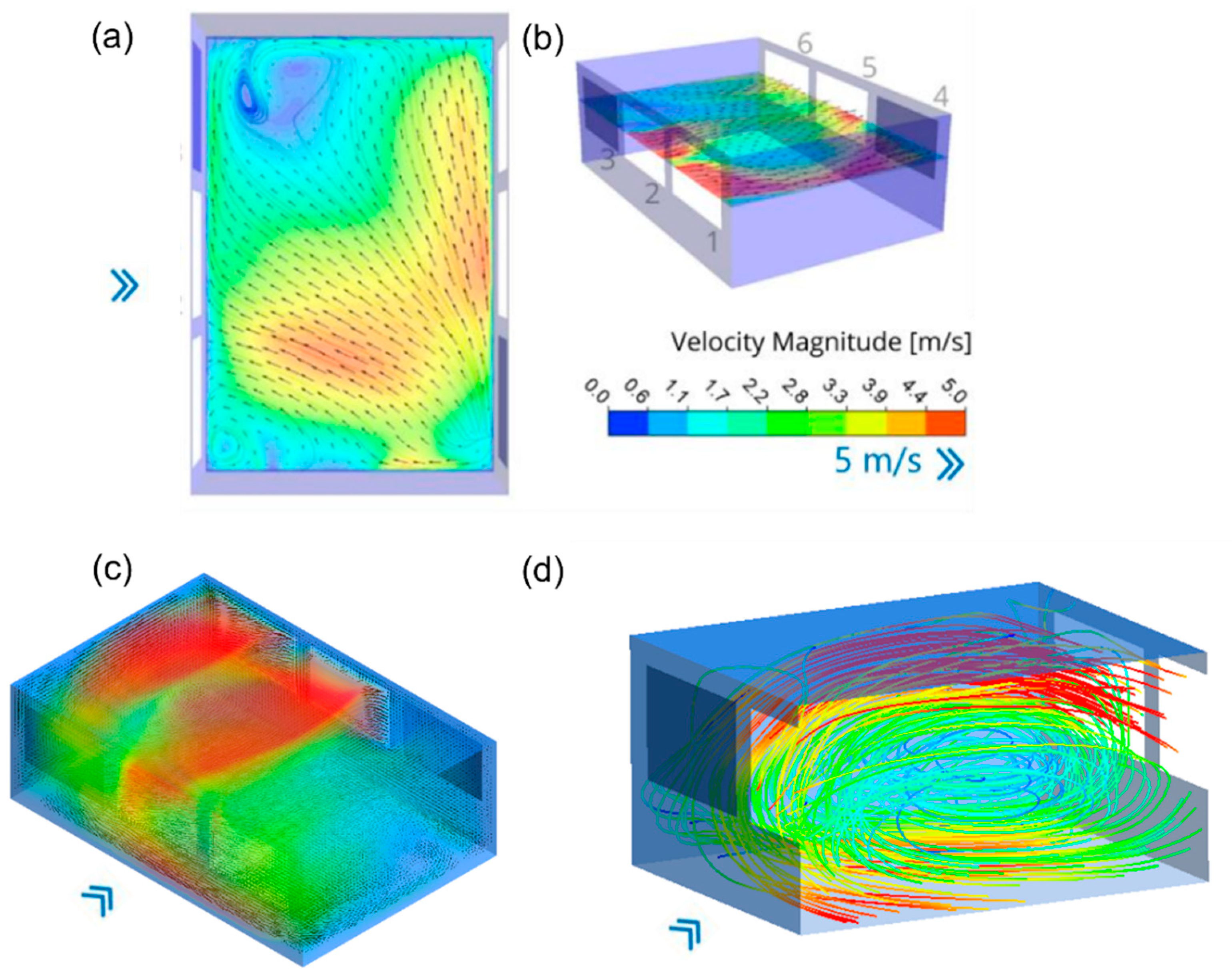
Figure 16.
Frame-by-frame analog visualization of Treatment T5 behavior, showing the movement of the polystyrene balls at different time instants: (a) start of the experiment, (b) 5 seconds, (c) 7 seconds, (d) 9 seconds, (e) 11 seconds, and (f) 13 seconds.
Figure 16.
Frame-by-frame analog visualization of Treatment T5 behavior, showing the movement of the polystyrene balls at different time instants: (a) start of the experiment, (b) 5 seconds, (c) 7 seconds, (d) 9 seconds, (e) 11 seconds, and (f) 13 seconds.
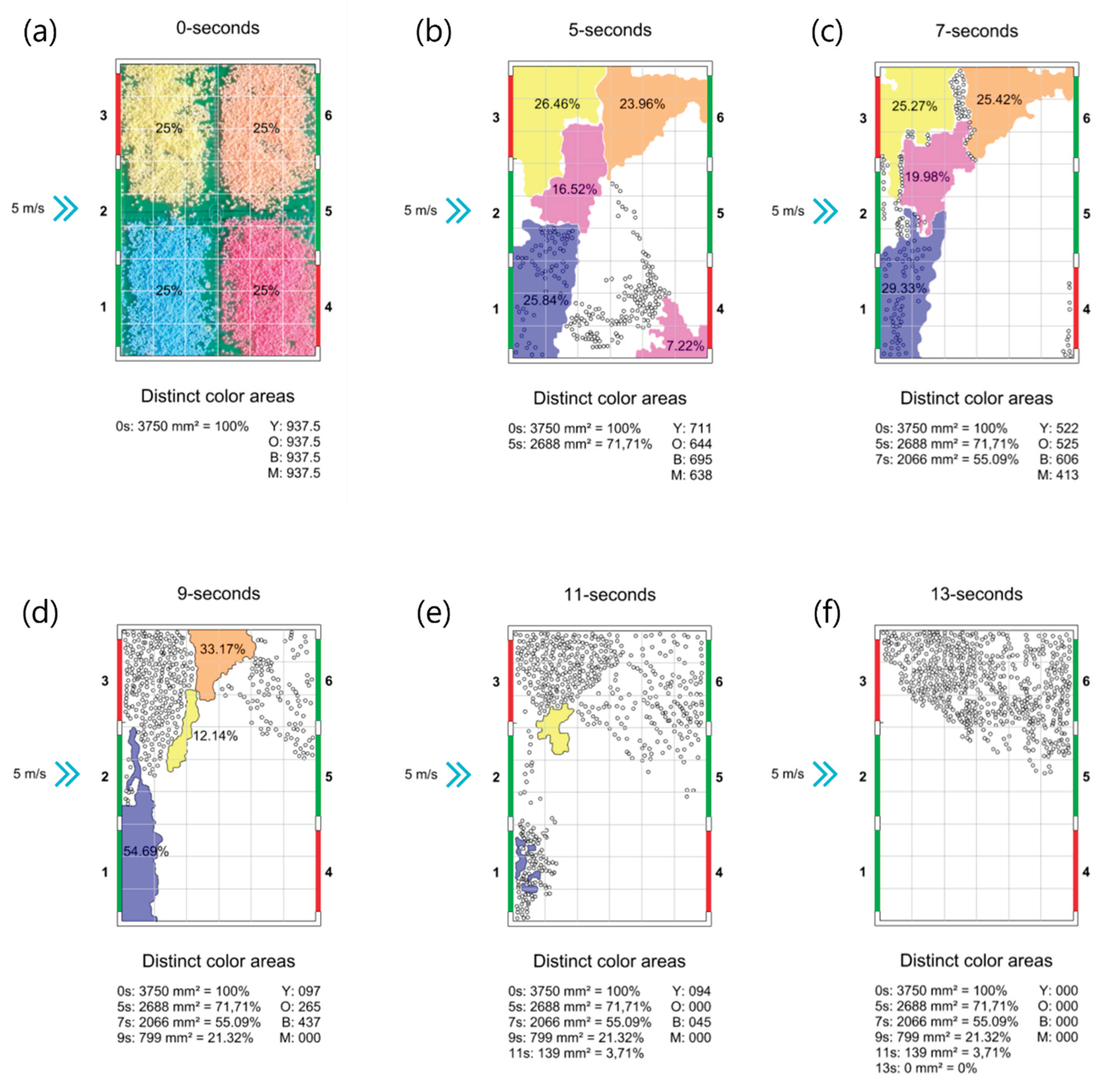

Table 1.
Unstructured tetrahedral mesh characteristics and parameters.
| Setting | Number of elements | Windward wall sizing | Prism layer |
|---|---|---|---|
| Mesh #1 | 400951 | ~8.7 x 10-³ | none |
| Mesh #2 | 540801 | ~7.8 x 10-³ | ~0.6 x 10⁻⁴ |
| Mesh #3 | 1216556 | ~4.5 x 10-³ | ~0.6 x 10⁻⁴ |
| Mesh #4 | 2719642 | ~3.3 x 10-³ | ~0.6 x 10⁻⁴ |
| Mesh #5 | 4344228 | ~2.7 x 10-³ | ~0.6 x 10⁻⁴ |
1 Source: Authors (2026).
Table 2.
Mesh parameters for the unstructured tetrahedral meshes settings.
| Setting | Inlet Windows | |||||
|---|---|---|---|---|---|---|
| W1 | W2 | W3 | ||||
| Experimental | 0.0396 | m³/s | 0.0383 | m³/s | 0.0386 | m³/s |
| k-e realizable | 0.0362 | 0.0349 | 0.0366 | |||
| W4 | W4 | W5 | ||||
| Experimental | 0.0423 | m³/s | 0.0248 | m³/s | 0.0409 | m³/s |
| k-e realizable | 0.0414 | 0.0246 | 0.0416 | |||
1 Source: Authors (2026).
Table 3.
Inferences derived from the comparison between empirical tests and numerical models.
 |
Disclaimer/Publisher’s Note: The statements, opinions and data contained in all publications are solely those of the individual author(s) and contributor(s) and not of MDPI and/or the editor(s). MDPI and/or the editor(s) disclaim responsibility for any injury to people or property resulting from any ideas, methods, instructions or products referred to in the content. |
© 2026 by the authors. Licensee MDPI, Basel, Switzerland. This article is an open access article distributed under the terms and conditions of the Creative Commons Attribution (CC BY) license (http://creativecommons.org/licenses/by/4.0/).
Copyright: This open access article is published under a Creative Commons CC BY 4.0 license, which permit the free download, distribution, and reuse, provided that the author and preprint are cited in any reuse.


