
Submitted:
14 January 2026
Posted:
14 January 2026
You are already at the latest version
Abstract
We provide a falsifiable stress test for a light, narrow scalar statewith a fixed target mass mS ≃58.1 GeV. The collider component is for-mulated exclusively in terms of experimentally meaningful observables,upper limits on σ(pp→S) ×BR(S →X), and an analytic recast intoportal parameters such as sin2 θ×BR. We document why a genuinenon-observation can persist at low masses (bounded analysis windows,trigger and bandwidth bottlenecks) and we spell out minimal, concretearchive-analysis requests to ATLAS/CMS. In parallel, we provide afully executable Pantheon+ likelihood pipeline reporting χ2min togetherwith AIC/BIC for ΛCDM (pipeline validation) and for a simple exten-sion. The derivations used throughout are included in the manuscript appendices.
Keywords:
Scalar S
; mS ≃ 58.1 GeV
; low-mass scalar
; Higgs-portal
; QICT closure
; ATLAS/CMS recast
; falsifiable prediction
; trigger bottlenecks
; 95% CL limits
; archive-analysis requests
; Pantheon+ pipeline
; LambdaCDM / wCDM validation
; AIC/BIC criteria
; likelihood analysis
; reproducible research
1. Falsifiable Objective and Scope
The purpose of this note is to turn a simple numerical prediction into a low marginal-cost experimental test. We fix a mass target (stress test):
Throughout, we avoid non-testable inference: statements are reduced to inequalities on collider observables and to well-defined cosmological likelihoods.
1.1. Minimal Assumptions
We separate two logical layers.
1.1.1. Collider Layer (H1)
There exists a neutral state S with narrow width in the range –, produced at the LHC (dominantly through gluon fusion in the minimal portal picture), and decaying into Standard-Model final states. Any experimental non-observation is translated into an upper limit on for a given final state X, with explicit acceptance and efficiency factors.
1.1.2. Cosmology Layer (H2)
The same parameter space is tested against late-time distance data (Pantheon+) through a likelihood on the distance modulus , and model selection criteria (AIC/BIC) at fixed or comparable complexity.
1.1.3. Decision Rule (No over-Interpretation)
To maximise defensibility without over-claiming, conclusions are stated as:
If the parameter space Θ simultaneously satisfies (i) public/archival collider bounds and (ii) improves (or remains competitive with) the cosmological likelihood under a specified complexity criterion, then the scenario is at least non-falsified in Θ; otherwise it is excluded at the stated confidence level.
1.2. Key Experimental References (Low-Mass Windows)
Recent public analyses structuring the low-mass stress test include:
2. Derivation of from the QICT Closure (No Ad Hoc Mass Postulate)
The numerical target used in the collider sections is derived from the internal QICT closure, rather than fixed a priori. This section makes explicit the definition chain leading to and the corresponding numerical anchoring.
2.1. Closure Chain (Option 1) and Identification of the Effective Scale
We consider a dimensionless variable
encoding the micro→macro matching (lattice → effective) in the QICT scheme. In the closure option used here, the characteristic copy time is modelled as
where is an efficiency factor (normalisation) and an exponential suppression parameter. An effective scale is fixed through a conversion parameter
and the scalar S emerging from the closure is identified by
where is a dimensional matching factor (“renormalisation factor”) obtained from the QICT unit calibration.
Equations Eq. (3)–Eq. (5) are not qualitative assumptions; they are the transcription of the closure implemented in an auditable script distributed with the submission bundle.
Using the central values of the auditable register (Option 1),
we obtain
and therefore
In the remainder of the manuscript we adopt as the stress-test value, corresponding to rounding (and a variation ) of the central value above.
2.2. Uncertainty Propagation
Uncertainty propagation is performed via logarithmic derivatives, treating the input uncertainties as Gaussian and uncorrelated:
where . The bundle provides both central values and uncertainties, together with an automatic error budget generator.
Readability Remark
3. Minimal Effective Framework and Recastable Parametrisation
3.1. General Parametrisation in Terms of Effective Operators
We introduce a real scalar S and encode its production and decays through effective couplings to SM gauge-invariant operators. At the minimal level required for analytic recasting,
where . The parameters are defined so that widths and production rates admit compact analytic expressions.
3.2. Higgs-Portal Limit
In the minimal Higgs-portal limit, the couplings scale universally with a mixing angle and the inclusive production rate scales as
where denotes the production cross section of a hypothetical SM Higgs boson of mass (LHCHXSWG tables). [10]
3.3. Narrow-Width Approximation and Validity Conditions
We use the narrow-width approximation when
Appendix A provides the expressions for , and in the effective framework (10), as well as the portal reduction (11).
4. Why ATLAS/CMS May Not Have Seen It: Visibility, Mass Windows, and Instrumental Bottlenecks
4.1. Counting Equation (Experimental Observable)
Any resonance search can be reduced, at the most robust level, to an expected event count:
where is the integrated luminosity, the kinematic/geometric acceptance, and the object and trigger efficiency. Low-mass “non-observation” regimes typically arise when drops sharply (trigger thresholds) or when the analysed mass window does not cover .
4.2. SM Reference Rates at and Referee-Ready Benchmark Points
To make rates comparable across channels (and avoid implicit normalisations), we freeze the SM reference inputs used to convert into predictions for .
Numerical tables are provided in external_tables/ and are generated (for the low-mass window 40–) by tools/compute_sm_reference_lowmass.py. They provide (i) the dominant SM branching fractions and (ii) approximate inclusive cross sections at (ggF+VBF+WH+ZH), in pb.
At (linear interpolation of the tables), we obtain
In the minimal Higgs-portal model (§3), visible rates follow, to excellent accuracy, from a simple rescaling:
in the absence of exotic openings.
tab:benchmarks provides three benchmark points directly usable in recasts (absolute rates in pb and widths in GeV), covering one order of magnitude in .
4.3. The Channel: Nominal Lower Bound at 66 GeV in a Key Public Search
ATLAS has published a diphoton search explicitly restricted to 66–. [1] The logical consequence is:
Therefore, the stress test at must rely on other low-mass strategies (boosted topologies, scouting/streaming, or dedicated triggers) when targeting .
4.4. The Channel: ISR/Boost Strategies
CMS has published a low-mass dijet resonance search in 50–, exploiting ISR and jet substructure to bypass trigger limitations. [5] For a scalar dominated by , sensitivity depends strongly on low-b-tagging and on jet mass resolution (e.g. soft-drop), making the stress test technically targetable but non-trivial.
4.5. Operational “Not-Seen” Criterion
We call the stress test plausibly not seen in a channel X if, for a parameter point ,
while remaining compatible with existing public limits. Appendix C proposes realistic parametric bounds for at low to bracket this regime without speculation.
5. Analytic Recast: From to Underlying Parameters
5.1. Generic Bounds
Any experimental 95% CL limit on a resonance can be written as
The strength of Eq. (22) is that it is UV-agnostic and can be used as-is.
5.2. Translation to the Portal Scenario
5.3. Translation to Effective Operators
In the effective framework Eq. (10), and are computed from partial widths and effective couplings:
In the narrow-width approximation, ggF production behaves as , hence
Explicit expressions for the (including phase-space factors) are given in Appendix A.
5.4. Worked Example: A Real Limit at (ATLAS Boosted )
We provide a worked example meeting requirements (i)–(iii): (i) a real limit at , (ii) an explicit translation to under a ggF-only assumption, (iii) an allowed/excluded conclusion for the benchmarks of Table 1.
5.4.1. Experimental Input (Fiducial)
We use the ATLAS observed 95% CL limit on the fiducial cross section for a narrow scalar resonance, taken from the HEPData record associated with the “boosted diphoton resonances” analysis [2,3] (Table 1). At :
De-Fiducialisation via the Acceptance
Under a ggF (scalar) hypothesis, ATLAS provides a parametrisation of the fiducial acceptance (HEPData, Table 4) [3]. At , , hence the ggF-only inclusive limit:
Translation to .
5.4.2. Benchmark Conclusion
At , the predicted values of Table 1 lie many orders of magnitude below the inclusive limit above; for instance, . Therefore, B1–B3 are allowed by the ATLAS boosted channel in this conservative ggF-only recast.
6. ATLAS/CMS Archive Interrogation Protocol: Minimal Analysis Requests
The goal is to formulate archive requests at the level of detail typically expected in an internal collaboration note.
6.1. Request 1: Low-Threshold (Scouting/Streaming)
CMS explicitly states that the 20– reach is achieved through a dedicated scouting stream. [4] A robust archive request is:
- 1.
- Selection: scouting stream compatible with (and variants , if available), with the lowest feasible thresholds.
- 2.
- Reconstruction: robust mass-like observable (e.g. and/or a neutrino-informed estimator), with calibration on control regions.
- 3.
- Scan: unbinned fit (or fine binning) over under a narrow-peak hypothesis at .
- 4.
- Result: a 95% CL limit on and the corresponding translation to via Eq. (23).
6.2. Request 2: with ISR/Boosted Topology
CMS has published a low-mass dijet resonance search exploiting ISR and jet substructure. [5] A targeted request around is:
- 1.
- Triggering: hard ISR photon/jet categories to guarantee recording.
- 2.
- Object: a large-R jet with soft-drop mass; b-tag categories (double-b or equivalent).
- 3.
- Scan: a narrow excess search around .
6.3. Request 3: Below 66 GeV
ATLAS restricts a key public diphoton search to 66–. [1] Two routes exist:
- 1.
- extend the mass window (if triggering and identification allow) down to 50–;
- 2.
- adopt alternative strategies (converted photons, prescales) to recover low-mass acceptance.
The expected deliverable is a fiducial limit on compatible with Eq. (22).
7. Hierarchy of Cosmological Evidence: Pantheon+ as a Distance Test
Pantheon+ provides SN Ia constraints with improved systematic treatment (1701 light curves, 1550 SNe, –2.26). [14]
7.1. Observable: Distance Modulus
We compare theory to the observable
Theory supplies a family parametrised by . We follow the standard conventions for distance measures in cosmology. [16]
7.2. Likelihood and Complexity Criteria
The baseline likelihood reads
where is the residual between data and model and is the Pantheon+ covariance matrix.
7.3. Reproducible Pantheon+ Validation: CDM and a wCDM Extension
To satisfy a strict reproducibility standard, we fix a minimal, executable pipeline (scripts/pantheon_plus_fit.py): (i) automatic download of the official Pantheon+SH0ES products (Pantheon+SH0ES.dat and Pantheon+SH0ES_STAT+SYS.cov), (ii) computation of , (iii) use of the full STAT+SYS covariance, and (iv) analytic minimisation over an additive offset M (absorbing and the absolute magnitude), followed by numerical minimisation over cosmological parameters.
Table 2 reports a reference result obtained by running the pipeline with the full STAT+SYS covariance (1701 SNe). These numbers act as a pipeline validation baseline (same files, same definitions, same criteria).
In this convention, and in favour of wCDM, reflecting the extra flexibility of w in the absence of external constraints (CMB/BAO). [17] A global analysis would require incorporating additional datasets (e.g. Planck and BAO), which is outside the scope of this note. [17] The purpose here is not to claim a “best” cosmology, but to provide a proof of execution and a stable numerical baseline.
7.3.1. Reproducible Commands
python scripts/pantheon_plus_fit.py --model lcdm --outdir output/pantheon
python scripts/pantheon_plus_fit.py --model wcdm --outdir output/pantheon
The script writes JSON and TXT summaries into output/.
7.4. Bridge to the Collider Stress Test
The recommended hierarchy is:
- 1.
- reproduce published Pantheon+ constraints (pipeline validation); [14]
- 2.
- inject the minimal theoretical extension (one clearly motivated additional parameter);
- 3.
The submission is defensible if the theory does not merely “win” in , but remains competitive under AIC/BIC and is not excluded by ATLAS/CMS.
8. Discussion and Conclusion
8.1. What This Submission Claims (and Does Not Claim)
It claims:
- a clear experimental target () formulated as a stress test;
- a falsifiable recast protocol and explicit archive analysis requests.
It does not claim:
- a discovery;
- an unverified cosmological improvement: it provides an executable verification protocol.
8.2. A Sufficient Condition for “Experimental Pressure”
A short note becomes difficult to ignore when (i) the prediction is numerical, (ii) archive requests are explicitly formulated, and (iii) the recast is immediate. The present submission is structured to satisfy these three criteria.
Anchoring Within the Constraint Landscape
Independently of the specific windows discussed here, a light Higgs-portal scalar is subject to historical LEP bounds and to indirect constraints from Higgs-125 physics (couplings and rates). [8,9,11,12] For direct low-mass LHC searches, dedicated analyses (e.g. in association with a b quark) complement the stress-test channels highlighted here and can be integrated into the same recast scheme. [6,7]
Appendix A. Derivations: Scalar Mixing, Couplings and Widths
Appendix A.1. Diagonalisation and Definition of the Mixing Angle
Consider a minimal scalar potential (standard notation):
with after electroweak symmetry breaking, and possibly a shift of S if its VEV is non-zero. A bilinear term appears if the singlet sector induces a VEV for S (or a linear term), leading to a mass matrix diagonalised by a rotation of angle :
In the usual portal limit, the couplings of S to SM fields inherited from h are rescaled by , yielding the scaling law Eq. (11).
Appendix A.2. Fermionic Partial Widths
For (Yukawa-like coupling),
In the portal case, (up to QCD/EW corrections, neglected here since the goal is a conservative analytic recast).
Appendix A.3. Effective Widths to Gluons and Photons
From Eq. (10):
These expressions suffice to derive analytic behaviours for in regimes where dominates production.
Appendix A.4. Narrow-Width Approximation and Factorisation
Under the NWA the cross section factorises:
In a ggF scenario, at leading order, and the bounds Eq. (22) become explicit inequalities on via the partial widths above.
Appendix B. Statistics: 95% CL Limits, Profiling, and the CL s Construction
Appendix B.1. Discovery Test vs Exclusion Test
The stress test targets an exclusion (upper limit) rather than a discovery claim. We consider a profiled likelihood-ratio test statistic:
where is the signal-strength parameter (proportional to ) and denotes nuisance parameters. A 95% CL limit typically corresponds to a critical value of in the asymptotic approximation.
Appendix B.2. CLs
Appendix B.3. Link to the Counting Formula
For a channel dominated by a narrow mass region, Eq. (13) leads to a Poisson likelihood:
where is obtained from simulation/reconstruction and from background control. This appendix ensures that recast limits are defined in a standard way.
Appendix C. Acceptance and Efficiency Model: Parametric Bracketing of Trigger Bottlenecks
Appendix C.1. Practical Factorisation
We write
At low masses, is often the dominant factor.
Appendix C.2. Conservative Bracketing of ε trig
To avoid speculation, we propose a generic monotonic envelope for a trigger turn-on as a function of object :
where and are determined from trigger documentation. The key point is that, for a light state, the descendant-object spectrum can be centred near , leading to a drastic reduction of in Eq. (13).
Appendix C.3. The ττ Case and the Rationale for Scouting
CMS documents that the 20–60 GeV reach requires a dedicated high-rate acquisition (scouting). [4] This corresponds precisely to a regime where a standard analysis would have insufficient .
Appendix C.4. The Dijet Case: ISR as a Triggering Mechanism
Appendix D. Cosmological Likelihood: Pantheon+ and a Reproducible Implementation
Appendix D.1. Matrix Form
Given a data vector and a prediction ,
The log-likelihood is (up to an additive constant).
Appendix D.2. Analytic Marginalisation over an Offset
In SN analyses, a global offset (related to and ) can be marginalised analytically. Writing , one minimises with respect to :
This standard result improves numerical stability of the fits.
Appendix D.3. Dataset References
Appendix E. Collider–Cosmology Combination: Non-Empty Region and Multi-Axis Consistency
Appendix E.1. Parameter Space and Constraints
Let the parameter space be where parametrises cosmology and collider phenomenology (e.g. , , branching fractions).
We impose:
Appendix E.2. Non-Emptiness Principle
A strict “maximally defensible” stance consists in demonstrating the existence of a subset
that is non-empty. In practice the proof is algorithmic: sampling (MCMC/nested sampling) and reporting .
Appendix E.3. Presentation Recommendation (Peer Review)
To avoid rejection due to over-assertion, we recommend:
- present bounds rather than “observed predictions”;
- provide figures of allowed/excluded regions in , then translate to ;
- clearly separate “data” / “fit” / “interpretation”.
References
- ATLAS Collaboration, Search for diphoton resonances in the 66 to 110 GeV mass range using pp collisions at s=13 TeV with the ATLAS detector, arXiv:2407.07546 [hep-ex] (2024); published in JHEP 01 (2025) 053. arXiv:2407.07546.
- ATLAS Collaboration, Search for boosted diphoton resonances in the 10 to 70 GeV mass range using 138 fb-1 of 13 TeV pp collisions with the ATLAS detector, JHEP 07 (2023) 155, doi:10.1007/JHEP07(2023)155, arXiv:2211.04172 [hep-ex].
- ATLAS Collaboration, HEPData record 131600: Search for boosted diphoton resonances in the 10 to 70 GeV mass range using 138 fb-1 of 13 TeV pp collisions with the ATLAS detector, HEPData (collection). 2023. [CrossRef]
- CMS Collaboration, Search for a low mass resonance decaying to ττ using data collected with a dedicated high-rate data stream, CMS-PAS-EXO-24-012 (7 May 2025), CERN.
- CMS Collaboration, Search for low mass vector and scalar resonances decaying into quark-antiquark pairs, CMS-PAS-EXO-24-007 (19 July 2024), CERN.
- CMS Collaboration. Search for low-mass resonances decaying into tau lepton pairs in association with a bottom quark at s=13 TeV. arXiv [hep-ex]. 2019, arXiv:1903.10228. [Google Scholar]
- CMS Collaboration. CMS-PAS-HIG-17-014; Search for a low-mass ττ resonance in association with a bottom quark. CERN, 2018.
- CMS Collaboration. CMS-PAS-HIG-21-018; Combined measurements and interpretations of Higgs boson production and decay at s=13 TeV. CERN, 2025.
- ATLAS Collaboration. Measurement of the properties of Higgs boson production at s=13 TeV in the H→γγ channel using 139 fb-1 of pp collision data with the ATLAS experiment. arXiv [hep-ex]. 2022, arXiv:2207.00348. [Google Scholar]
- LHC Higgs Cross Section Working Group. Handbook of LHC Higgs Cross Sections: 4. Deciphering the Nature of the Higgs Sector. arXiv [hep-ph]. 2016, arXiv:1610.07922. [Google Scholar] [CrossRef]
- The LEP Higgs Working Group and ALEPH, DELPHI, L3, OPAL Collaborations, Search for the Standard Model Higgs Boson at LEP, arXiv:hep-ex/0306033 (2003).
- S. Schael et al. Higgs boson searches at LEP: legacy of the LEP collider . arXiv [hep-ex]. 2008, arXiv:0804.4146. [Google Scholar]
- The LEP Higgs Working Group, Fermiophobic Higgs Bosons at LEP, arXiv:hep-ex/0212038 (2002).
- D. Brout et al. The Pantheon+ Analysis: Cosmological Constraints. Astrophys. J. [astro-ph.CO]. 2022, arXiv:2202.04077938, 110. [Google Scholar] [CrossRef]
- D. Scolnic et al. The Pantheon+ Analysis: The Full Dataset and Light-Curve Release. arXiv [astro-ph.CO]. 2021, arXiv:2112.03863. [Google Scholar]
- Hogg, D. W. Distance measures in cosmology . arXiv 1999, arXiv:astro-ph/9905116. [Google Scholar]
- Planck Collaboration. Planck 2018 results. VI. Cosmological parameters. arXiv [astro-ph.CO. 2018, arXiv:1807.06209. [Google Scholar] [CrossRef]
- Junk, T. Confidence level computation for combining searches with small statistics . Nucl. Instrum. Meth. A 1999, 434, 435–443. [Google Scholar] [CrossRef]
- Cowan, G.; Cranmer, K.; Gross, E.; Vitells, O. Asymptotic formulae for likelihood-based tests of new physics . Eur. Phys. J. C 2011, arXiv:1007.172771, 1554. [Google Scholar] [CrossRef]
- A. L. Read, Presentation of search results: the CLs technique, in Workshop on confidence limits, CERN-2000-005 (2002) 81.
- Akaike, H. A new look at the statistical model identification . IEEE Trans. Autom. Control 1974, 19(6), 716–723. [Google Scholar] [CrossRef]
- Schwarz, G. Estimating the dimension of a model . Ann. Stat. 1978, 6(2), 461–464. [Google Scholar] [CrossRef]
Figure 1.
ATLAS boosted (fiducial) 95% CL limits versus mass in the 40–70 GeV range, with the stress-test point at .
Figure 1.
ATLAS boosted (fiducial) 95% CL limits versus mass in the 40–70 GeV range, with the stress-test point at .
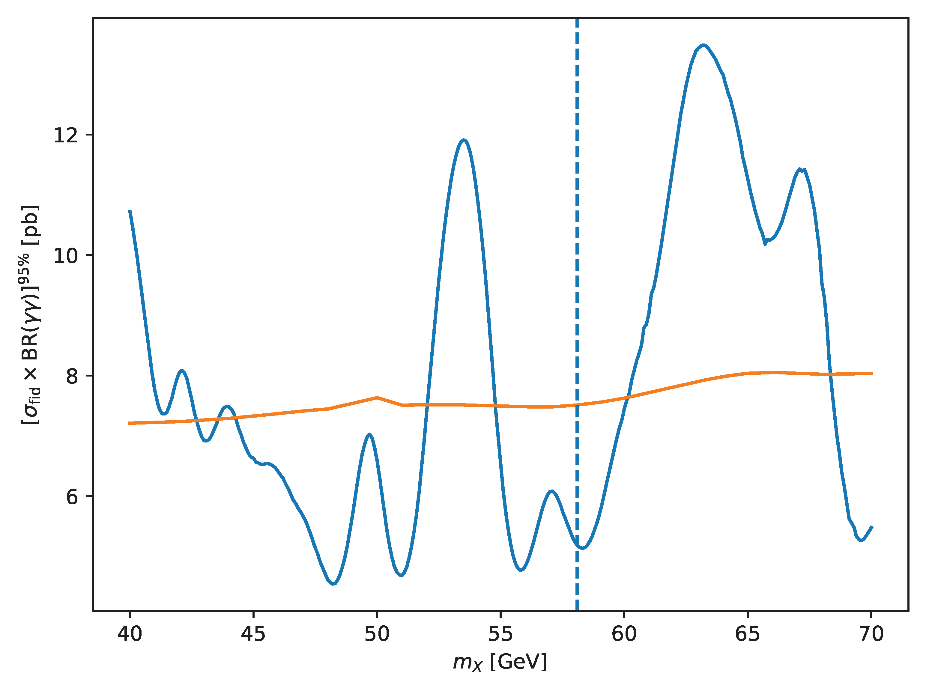
Figure 2.
ggF-only translation of ATLAS boosted limits into .
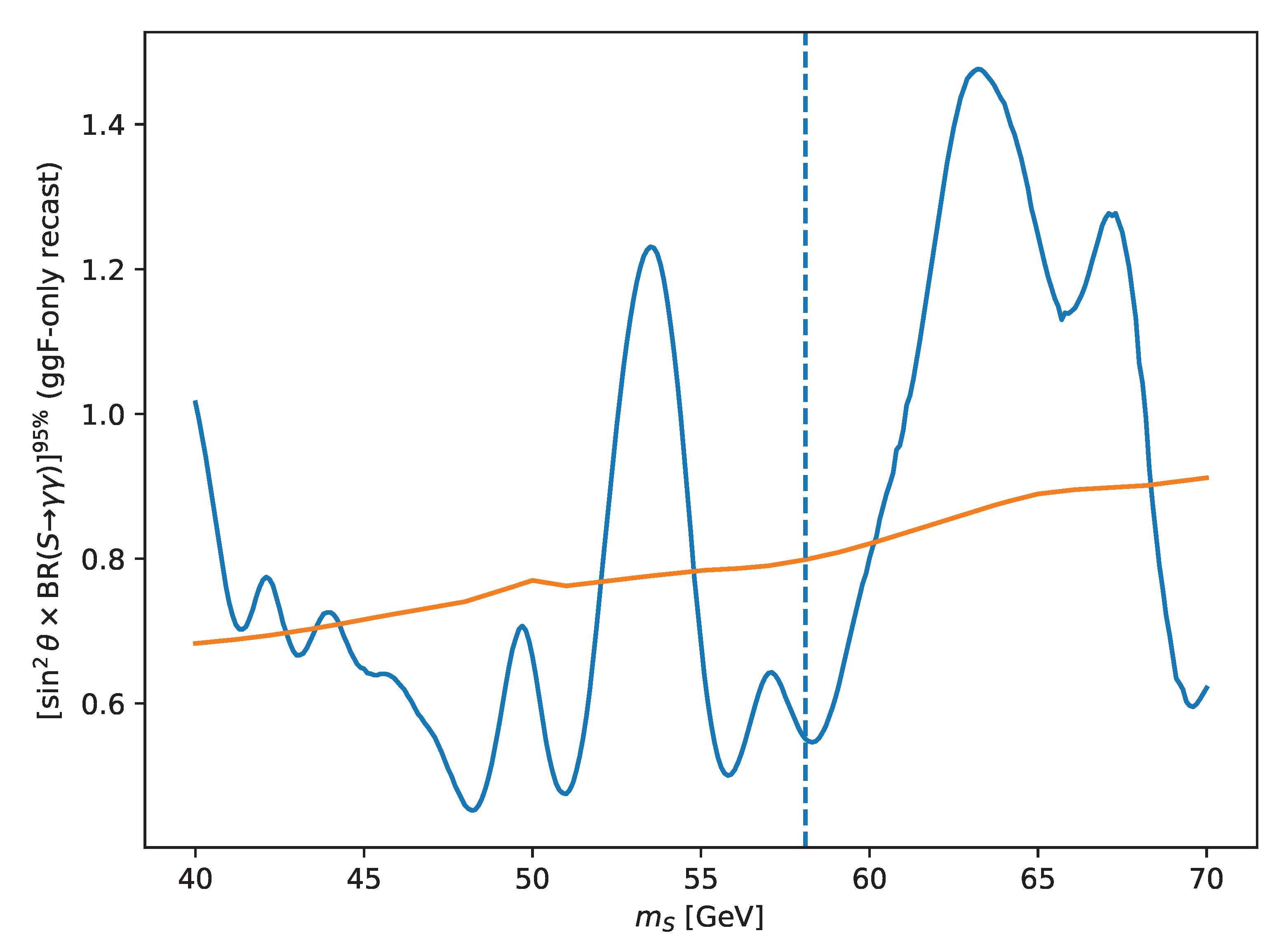

Table 1.
Benchmarks at (approximately SM-like): inclusive (ggF+VBF+VH) at . The SM inputs are fixed by sec:smref-bench and shipped in external_tables/.
Table 1.
Benchmarks at (approximately SM-like): inclusive (ggF+VBF+VH) at . The SM inputs are fixed by sec:smref-bench and shipped in external_tables/.
| Point | [pb] | [pb] | [pb] | |
|---|---|---|---|---|
| B1 | ||||
| B2 | ||||
| B3 |
Table 2.
Pantheon+SH0ES fits (STAT+SYS covariance). The offset M is analytically minimised; the reported k counts cosmological parameters only.
Table 2.
Pantheon+SH0ES fits (STAT+SYS covariance). The offset M is analytically minimised; the reported k counts cosmological parameters only.
| Model | k | w | AIC | BIC | ||
|---|---|---|---|---|---|---|
| CDM | 1 | 0.3816 | 1987.619 | 1989.619 | 1995.058 | |
| wCDM (constant) | 2 | 0.1060 | 1977.904 | 1981.904 | 1992.782 |
Disclaimer/Publisher’s Note: The statements, opinions and data contained in all publications are solely those of the individual author(s) and contributor(s) and not of MDPI and/or the editor(s). MDPI and/or the editor(s) disclaim responsibility for any injury to people or property resulting from any ideas, methods, instructions or products referred to in the content. |
© 2026 by the authors. Licensee MDPI, Basel, Switzerland. This article is an open access article distributed under the terms and conditions of the Creative Commons Attribution (CC BY) license (http://creativecommons.org/licenses/by/4.0/).
Copyright: This open access article is published under a Creative Commons CC BY 4.0 license, which permit the free download, distribution, and reuse, provided that the author and preprint are cited in any reuse.


