Submitted:
09 January 2026
Posted:
12 January 2026
You are already at the latest version
Abstract
A retrospective ozone simulation was conducted with the Microscale Forward and Adjoint Chemical Transport (MicroFACT) model for an industrialized area of Detroit, Michigan, USA using a 24 km × 24 km horizontal × 1.5 km vertical grid. The domain encompassed a regulatory monitoring station at East 7 Mile Rd at the northern edge of the grid. The episode day was 30 June 2022, when the station-measured 8-hour ozone reached 76 ppb during predominantly southwesterly wind. The ozone impacts of mobile, point, nonpoint, and biogenic emissions were simulated at 400 m horizontal resolution. Simulation results were compared against station measurements of ozone, nitrogen oxides, and total reactive nitrogen. Local nitrogen oxide sources were found to titrate ozone, while ozone turbulently entrained to the surface from ~500 m aloft enhanced surface Ozone Production Efficiency and led to extended periods of high ozone concentrations very similar to observations. Volatile Organic Compound emission reductions produced only weak decreases in maximum 8-hour ozone, suggesting that radicals were enhanced mostly by photolysis of subsiding ozone. Entrainment of ozone layers aloft may thus be critical in explaining historical ozone exceedances of the United States National Ambient Air Quality Standard at the East 7 Mile Rd station.
Keywords:
ozone
; air quality
; modeling
; atmospheric chemistry
; ozone production efficiency
; nitrogen oxides (NOx)
; reactive nitrogen (NOy)
; volatile organic compounds (VOC)
1. Introduction
The United States (U.S.) National Ambient Air Quality Standard (NAAQS) for ozone (O3) is based on the maximum daily eight-hour average (8-h) O3 concentration (MDA8 O3) measured at a monitoring station, and is currently set by the U.S. Environmental Protection Agency (USEPA, Washington, DC, U.S.) at 70 parts per billion by volume (ppb) [1]. Attainment of the NAAQS is based on the three-year average of the annual 4th highest MDA8 O3, referred to as the design value. Areas with design values that exceed the NAAQS at any station may be designated by the USEPA as in nonattainment of the O3 standard within several categories of increasing seriousness from marginal to severe. In 2023, Southeast Michigan (SEMI) in the U.S. Great Lakes region, including the City of Detroit, was re-designated by the USEPA from moderate O3 nonattainment to attainment based on a clean data determination for the three-year period of 2020-2022. This determination was partly based on an exceptional event demonstration by the State of Michigan attributing two days of high O3 values in June 2022 to a Canadian wildfire.
SEMI’s attainment status could be impacted by a regulatory monitoring site located at East 7 Mile Rd in the City of Detroit. Fine-scale O3 modeling for the Detroit area was performed with the Microscale Forward and Adjoint Chemical Transport (MicroFACT) model [2] to understand the impacts of local emission sources on ambient O3 at East 7 Mile Rd station. The results may help to guide the selection of emission controls or other measures to attain the O3 NAAQS in any future required State Implementation Plan.
This study examines an O3 episode on 30 June 2022. During this episode, winds were predominantly from the southwest (the typical wind direction for MDA8 O3 above 70 ppb in SEMI), with no forest fire smoke or lake breeze influence as determined from satellite imagery. Figure 1 shows twelve-hour (12-h) back trajectories arriving at or 500 m above the East 7 Mile Rd station at 14:00 Local Standard Time (LST), 30 June 2022 generated by the Hybrid Single-Particle Lagrangian Integrated Trajectory (HYSPLIT) model [3]. These trajectories indicate two things: 1) the potential for regional transport of O3 and its precursors from industrialized areas not only in Michigan, but also in the neighboring states of Ohio and Indiana; and 2) the likelihood of elevated layers of enhanced O3 due to the greater distance traveled over the industrialized U.S. Midwest by air parcels aloft relative to air parcels near the surface. MDA8 O3 at East 7 Mile Rd station on 30 June 2022 was 76 ppb. While this concentration was the highest for the year in SEMI, it is not regulatorily significant because design values are based on the 4th highest MDA8 O3. Nevertheless, understanding the physical mechanism behind the high O3 measured during this episode may reveal insights useful to the design of future O3 control strategies, if needed.
The EGLE monitoring network in SEMI includes the Allen Park station located to the southwest of East 7 Mile Rd (Figure 2), upwind of the latter during the 30 June 2022 episode. Between the two stations is the most heavily industrialized area in Michigan (Figure 3), including two natural gas-fired power plants (DG, DT), a refinery (MP), three automotive assembly facilities (FD, MA, JN), two steel mills (US, CC), a coking facility (ES), a lime plant (CL), a large wastewater treatment plant (WW), and a hazardous waste storage and treatment facility (UE). MDA8 O3 at Allen Park station during the O3 episode was 71 ppb, 5 ppb less than at East 7 Mile Rd., a concentration possibly influenced by long-range transport. The question addressed by this study is whether the O3 gradient observed between the two stations on 30 June 2022 was due to the significant concentration of local emission sources downwind of Allen Park, and whether emission reductions at these sources would be beneficial as potential control strategies.
2. Methods
The MicroFACT model [2] used for this study is a sub-km horizontal resolution 3D Eulerian grid model with forward and inverse modes, the latter based on the 4D variational data assimilation technique [4,5]. It is driven by 3D building-sensitive winds derived from Los Alamos National Lab’s Quick Urban Industrial Complex (QUIC) model [6]. MicroFACT simulates pollutant transport by advection and turbulent diffusion, while chemistry is simulated with 116 gas-phase and 7 heterogeneous reactions. For this study, the recent parameterization of nitrous acid (HONO) formation based on smog chamber experiments by Song et al. [7] was added to the chemical mechanism to enhance radical production and HONO concentrations in line with recent field measurements [8]. The clear sky photolysis rates calculated using the method of Saunders et al. [9] were also enhanced for the effects of surface albedo on NO2 and O3 photolysis, assuming for simplicity that direct radiation dominates the former and diffuse radiation the latter [10].
MicroFACT can not only predict atmospheric concentrations of pollutants based on specified emissions but can also infer emissions at fine scale from ambient air concentrations. Olaguer previously used MicroFACT to perform inverse modeling of formaldehyde (HCHO) emissions from industrial and mobile sources [11] and methane emissions from natural gas pipeline leaks [12] based on mobile lab measurements during the 2021 Michigan-Ontario Ozone Source Experiment (MOOSE) [13] within the area shown in Figure 2.
For this study, MicroFACT was applied to a 24 km × 24 km, 400 m resolution horizontal grid as shown in Figure 3. The vertical grid had 20 layers from 0 to 1500 m above ground level, with parabolically increasing layer thickness with height (2 m at surface). The horizontal resolution of MicroFACT as implemented in this study is 10 times the typical highest resolution of regional air quality models used for regulatory applications in the U.S. Figure 3 shows contours of modeled O3 concentration at 14:00 LST, 30 June 2022, the time of maximum hourly average O3 simulated by MicroFACT at East 7 Mile Rd (see Table A1 in Appendix A). Note the significant horizontal gradients in O3 apparent at fine scale that would be unresolved by coarser resolution models.
The QUIC model was used to generate hourly 3D wind fields consistent with flow around buildings at 20 m horizontal resolution based on background wind and other meteorological measurements at the Detroit Metropolitan Wayne County Airport (DTW) in Romulus, Michigan, roughly 10 km to the southwest of Allen Park. Airport measurements were run through the EPA AERMET pre-processor [14] to produce hourly values for wind speed and direction as well as turbulence parameters required by QUIC. The resulting 3D winds were then averaged and staggered with respect to the MicroFACT grid to ensure mass conservation (i.e., an Arakawa C-grid [15]). Figure 4 shows wind streamlines at 1 m above ground level generated by the QUIC model for 14:00 LST, 30 June 2022.
Hourly vertical temperature profiles in the domain interior were based on measurements at the Windsor International Airport (YQG) in Ontario, Canada located within the model grid. These measurements were processed with AERMET to produce boundary layer parameters required to infer atmospheric thermal structure. In the convectively unstable or neutral cases the temperature profile was based on the observed lapse rate. In the stable case, it was computed based on the Monin-Obukhov length, the surface heat flux, the roughness length, the friction velocity, and the inversion height [16].
U.S. annual point source emissions for 2022 and associated stack parameters were specified from Michigan’s State and Local Emissions Inventory System [17] with speciation based on the EPA Emissions Modeling Platform [18]. Point source emissions for Windsor, Ontario were supplied by Environment and Climate Change Canada (ECCC) for the available year 2017. Hourly mobile source emissions were based on 2022 runs of the USEPA Motor Vehicle Emission Simulator (MOVES) [19] by the Lake Michigan Air Directors Consortium (LADCO), while hourly biogenic emissions were based on LADCO 2022 runs of the Biogenic Emission Inventory System (BEIS) [20]. For 2022 nonpoint sources, annual combustion emissions were obtained from Wayne County, Michigan, while speciated Volatile Organic Compound (VOC) emissions from consumer and commercial products were obtained from the USEPA. Road lengths and population were used as surrogates to distribute emissions among the 400 m × 400 m grid cells. Note that point source emissions of HCHO were adjusted based on known HCHO:CO emission ratios (2-5%) according to the method described by Olaguer et al. [21], to be consistent with the findings of the MOOSE study regarding industrial primary HCHO [11,21].
Hourly species boundary conditions for 35 advected species and surrogates for lumped species (e.g., NO3X = NO3+N2O5) were derived by combining measurements at Allen Park for surface O3, CO, and total reactive nitrogen (NOy) and simulated 1D vertical profiles at the same location from regional air quality models, specifically ECCC’s GEM-MACH [22] (2.5-km resolution for O3, CO, HCHO, ethene, and most NOy species) and a LADCO run of CAMx [23] (4-km resolution for most organic species and NO3X). While GEM-MACH had higher horizontal resolution than CAMx, the latter model’s lumping scheme for organic species was closer to that of MicroFACT, hence the necessity of separate sources for the boundary conditions.
Vertical ozone profiles derived from ozone sondes, ozone lidars, ground-based multi-axis differential optical absorption spectrometers, and satellites often show elevated layers of enhanced tropospheric ozone exceeding surface concentrations at altitudes below 1 km during pollution events in the planetary boundary layer [24,25,26,27]. Hourly O3 profiles from the GEM-MACH model showed enhanced layers aloft in the late morning and afternoon, but with lower concentrations at the surface than measured at Allen Park (see Appendix B). The difference between the measured surface concentration and the GEM-MACH value was uniformly added throughout the vertical column to preserve the modeled layer structure (Table B1). Similar adjustments were made for CO and NOy, with the latter distributed proportionally among relevant species (Table B2 and Table B3). Pollutants aloft were entrained to the surface as the planetary boundary layer expanded based on the vertical diffusivity parameterization of Delle Monache et al. [28] and boundary layer parameters derived from YQG airport data. Figure 5 shows the ozone boundary condition and the accompanying vertical diffusivity profile at 14:00 LST, 30 June 2022.
The simulation period was 5:00 to 19:00 LST with 20 s time steps. Initial conditions for species concentrations were set equal to the boundary conditions at 5:00 LST. The spin-up period consisted of the first four hours, during which the initial conditions were advected out of the domain (at a typical wind speed of ~3 m/s) and replaced by more realistic species concentrations consistent with local emissions and chemistry. Because of the low nocturnal mixing height, urban morphology was ignored in the wind field during the first hour to avoid computational instability due to taller structures in downtown Detroit. The ten-hour (10-h) period beyond spin-up from 9:00 to 19:00 LST coincided with measured O3 concentrations at East 7 Mile Rd above 60 ppb (Table A2).
3. Results
The model inputs described above define the base case configuration. The simulation results for the base case were compared with measurements at the East 7 Mile Rd station for O3, NO, NO2, odd oxygen (O3 + NO2), and NOy, as illustrated in Table 1 and Table 2 for the hours when observed O3 exceeded 60 ppb. In these tables, the Normalized Mean Bias (NMB) was computed as the average of the difference between the modeled and measured hourly concentrations over the appropriate 8-h or 10-h period, divided by the corresponding measured 8-h or 10-h concentration. Comparisons between modeled concentrations and measurements for the individual hours are displayed in Table A1, Table A2 and Table A3.
MicroFACT successfully simulated 8-h O3 for the periods when observed O3 exceeded 60 ppb, although the simulated MDA8 O3 occurred at 9:00 – 17:00 LST, whereas the observed MDA8 O3 occurred at 11:00 – 19:00 LST. Reactive nitrogen species were over-predicted relative to observations, while the simulated odd oxygen (Ox) agreed well with observations (within 10%) despite the errors in NOy species. The hourly comparison presented in Appendix A shows that the model underpredicted O3 relative to observations in the hours just before sunset but compensated for this by overpredicting NO2. During the real episode, the buildup of reactive nitrogen was prevented in the later hours of the day while O3 remained at or above 75 ppb despite the weakening of photolytic conversion of NO2 to O3. The observed behavior of O3 towards evening was perhaps due to greater persistence of O3 entrainment from aloft in reality compared to the simulation.
The overprediction of NOy was possibly due to errors in nitrogen oxide (NOx = NO + NO2) emissions or chemical loss mechanisms. In contrast, 2016 CMAQ model simulations of summertime NOx by the USEPA for the continental U.S. have late morning to late afternoon NMB values roughly between -15% and -30% [29]. The discovery of much higher observed ratios of HONO:HNO3 than simulated by current models during the MOOSE study [13] may indicate fundamental deficiencies in our current understanding of NOy emissions and chemistry. Despite the inclusion of heterogeneous reactions on both aerosol and ground surfaces, a specified ratio of aerosol surface area to air volume of 0.0014 m2 m−3 at the high end of measured values in the U.S. [30], and the addition of the HONO parameterization of Song et al. [7] in MicroFACT, the model did not generate HONO:HNO3 ratios above 0.4, compared to mean ratios of 3 measured in Detroit during MOOSE.
Nitrous acid formation is closely tied to poorly understood heterogeneous chemical processes that may play an essential role in regulating the NOy budget in urban airsheds. Akimoto and Tanimoto [31] noted frequent reports of disagreement between observations and corresponding air quality model simulations of HONO and HNO3. They called for comprehensive field study measurements of NOy species to improve the simulation of chemical processes in atmospheric models, with special emphasis on heterogeneous “renoxification” reactions involving HONO and HNO3.
In addition to the base case simulation, a sensitivity experiment was conducted in which enhanced O3 layers aloft were suppressed when surface O3 at Allen Park exceeded 60 ppb. The measured hourly concentration at Allen Park in this case was set as the maximum value aloft in the O3 boundary conditions. The result was that the modeled MDA8 O3 at East 7 Mile Rd decreased by 15 ppb to 63 ppb, well below the value at Allen Park. This was because NOx sources between Allen Park and East 7 Mile Rd titrated O3 (which is recovered when NO2 produced by NO titration of O3 photolyzes further downwind), an effect diluted by the coarser resolution of regional air quality models. In the base case, O3 entrained from aloft countered this titration by adding directly to surface O3 and by increasing the production of radicals through the photolysis of subsiding ozone followed by H2O + O(1D) → 2OH. This is illustrated in Table 3 below, which shows differences in Ozone Production Efficiency (OPE) between the sensitivity experiment and the base case, as well as corresponding differences in O3 and Ox averaged over 9:00 – 19:00 LST.
The OPE, defined by Chace et al. [32] as the slope of the linear regression between odd oxygen and reactive nitrogen reservoirs (NOz = NOy – NOx), roughly indicates the amount of O3 eventually generated per NOx molecule through conversion of NO to NO2 by atmospheric radicals before NOx is terminated and stored in NOz. Note how the OPE decreased by almost half between the base case and the sensitivity experiment. For comparison, the corresponding OPE computed from station measurements was 15.4, which may indicate that downward mixing of O3 from aloft was even stronger than simulated by MicroFACT, especially late in the day.
In addition to the sensitivity experiment described above, additional experiments were conducted involving hypothetical emission reductions of NOx (10%) and VOCs (10% and 50%) at stationary sources. These experiments are summarized in Table 4 below.
Clearly, NOx titration results in an increase in O3 due to NOx reduction, so that local O3 is radical-limited rather than NOx-limited [33]. The weak impact of VOC reductions indicates that VOCs are not the major source of radicals compared to O3 entrained from aloft. This does not rule out, however, that local VOC and NOx controls may result in O3 reductions further downwind of East 7 Mile Rd under southwesterly flow. It is also possible that emission reductions upwind of Allen Park but still within the SEMI region may decrease MDA8 O3 at Allen Park and East 7 Mile Rd by mitigating O3 transport aloft.
4. Discussion and Conclusions
Based on station measurements at Allen Park and East 7 Mile Rd, and corresponding MicroFACT and trajectory model simulation results for the 30 June 2022 O3 episode in Detroit, Michigan, the following conclusions may be drawn:
- Local emission sources between Allen Park and East 7 Mile Rd tend to reduce MDA8 O3 at the latter station below the corresponding concentration at Allen Park due to NOx titration of O3.
- Pollution layers aloft may counter O3 titration when they are turbulently entrained to the surface, thus adding directly to ground-level O3 and enhancing radical concentrations and O3 production efficiency.
- Transport of O3 around 500 m above ground level may significantly contribute to MDA8 O3 above 70 ppb at East 7 Mile Rd during southwesterly wind flow that imports pollution from a wide region in the U.S. Midwest.
MicroFACT was able to demonstrate the above mechanism for the O3 episode because of the model’s fine-scale resolution relative to coarser-resolution regional models, which dilute the NOx titration effect and underestimate O3 concentrations aloft by artificially diffusing plumes. The fine-scale simulation results show the importance of routine measurements of O3 vertical profiles and boundary layer mixing height to enable evaluation of elevated pollution layers and their entrainment to the surface. Unfortunately, such measurements were unavailable for this study. (Note that a ceilometer is normally operated at the East 7 Mile Rd station. However, the instrument was offline on 30 June 2022.)
More explicit coupling between regional and fine-scale air quality models may improve our understanding of the physical mechanisms involved in high O3 episodes in SEMI. Among the uncertainties that require further examination in future simulations of O3 episodes are the details of NOy chemistry, especially heterogeneous production and loss mechanisms that may limit NOy concentrations before sunset.
While local VOC and NOx controls in the modeled area may not significantly mitigate MDA8 O3 at East 7 Mile Rd, SEMI at large may still be VOC-sensitive [34], so that a combination of VOC controls over a wider area and continued U.S. national reductions in NOx emissions may help ensure O3 attainment in SEMI by reducing either near-regional or longer-range O3 transport in the lower planetary boundary layer.
Author Contributions
Conceptualization, E.P.O., methodology, E.P.O., M.V.; investigation, E.P.O.; writing—original draft preparation, E.P.O.; writing—review and editing, E.P.O., M.V.; project administration, E.P.O.; funding acquisition, E.P.O. All authors have read and agreed to the published version of the manuscript.
Funding
This research was funded by the USEPA, Washington, DC, USA, grant number E03423.
Institutional Review Board Statement
Not applicable.
Informed Consent Statement
Not applicable.
Data Availability Statement
Data from this study are available upon request from the corresponding author.
Acknowledgments
Jim Haywood of EGLE processed airport data and provided Figure 1. Mark Janssen of LADCO, Junhua Zhang of ECCC, and Havala Pye and Karl Seltzer of USEPA provided emissions data. Tsengel Nergui of LADCO and Craig Stroud of ECCC provided boundary conditions from runs of the CAMx and GEM-MACH models respectively. Robert Goodwin of Michigan State University provided the 3D building shapefile used as input to the QUIC model.
Conflicts of Interest
The authors declare no conflict of interest.
Appendix A
The following tables compare the simulated and observed evolution of hourly average (1-h) species concentrations for 9:00 – 19:00 LST, 30 June 2022 at East 7 Mile Rd. Table A1 displays 1-h species concentrations simulated by the MicroFACT model for the base case, while Table A2 shows corresponding station measurements. Table A3 displays relative differences between the modeled and measured 1-h concentrations. Note the persistence of measured O3 exceeding 70 ppb compared to model concentrations later in the day, as well as lower observed concentrations of NOy compared to simulated values.

Table A1.
1-h concentrations (ppb) simulated by MicroFACT at East 7 Mile Rd for 30 June 2022.
| Species | 9:00– 10:00 LST | 10:00 – 11:00 LST | 11:00 – 12:00 LST | 12:00 – 13:00 LST | 13:00 – 14:00 LST | 14:00 – 15:00 LST | 15:00 – 16:00 LST | 16:00 – 17:00 LST | 17:00 – 18:00 LST | 18:00 – 19:00 LST |
| NO | 2.4 | 1.5 | 1.5 | 1.5 | 1.8 | 1.5 | 2.1 | 3.1 | 3.9 | 4.5 |
| NO2 | 7.4 | 6.0 | 6.0 | 6.7 | 7.5 | 8.1 | 10.0 | 12.6 | 15.0 | 22.1 |
| O3 | 66.4 | 76.8 | 82.6 | 82.0 | 81.1 | 84.9 | 79.5 | 73.9 | 62.2 | 48.4 |
| Ox | 73.8 | 82.8 | 88. 6 | 88.7 | 88.6 | 93.0 | 89.4 | 86.5 | 77.2 | 70.5 |
| NOy | 15.0 | 12.6 | 11.1 | 11.1 | 11.6 | 11.8 | 14.5 | 18.3 | 21.3 | 29.6 |
Table A2.
Measured 1-h concentrations (ppb) at East 7 Mile Rd on 30 June 2022.
| Species | 9:00– 10:00 LST | 10:00 – 11:00 LST | 11:00 – 12:00 LST | 12:00 – 13:00 LST | 13:00 – 14:00 LST | 14:00 – 15:00 LST | 15:00 – 16:00 LST | 16:00 – 17:00 LST | 17:00 – 18:00 LST | 18:00 – 19:00 LST |
| NO | 1 | 0.8 | 0.2 | 0.2 | 0.2 | 0.1 | 0.2 | 0.1 | 0.2 | 0.1 |
| NO2 | 6.1 | 5.1 | 2.2 | 2.1 | 2.1 | 1.7 | 2 | 2.3 | 2.6 | 2.5 |
| O3 | 61.1 | 67.7 | 71 | 72.4 | 75.6 | 77.7 | 77.9 | 80.9 | 79 | 75 |
| Ox | 67.2 | 72.8 | 73.2 | 74.5 | 77.7 | 79.4 | 79.9 | 83.2 | 81.6 | 77.5 |
| NOy | 9.4 | 8.2 | 4.4 | 4.3 | 4.3 | 3.8 | 4.2 | 4.6 | 4.9 | 4.7 |
Table A3.
Relative differences (%) between modeled and measured 1-h concentrations at East 7 Mile Rd for 30 June 2022.
Table A3.
Relative differences (%) between modeled and measured 1-h concentrations at East 7 Mile Rd for 30 June 2022.
| Species | 9:00– 10:00 LST | 10:00 – 11:00 LST | 11:00 – 12:00 LST | 12:00 – 13:00 LST | 13:00 – 14:00 LST | 14:00 – 15:00 LST | 15:00 – 16:00 LST | 16:00 – 17:00 LST | 17:00 – 18:00 LST | 18:00 – 19:00 LST |
| NO | 142.4 | 92.1 | 639.9 | 640.7 | 808.4 | 1393.6 | 954.3 | 3012.6 | 1831.1 | 4380.2 |
| NO2 | 21.5 | 18.2 | 170.6 | 218.0 | 257.6 | 377.3 | 399.0 | 448.0 | 475.3 | 782.9 |
| O3 | 8.6 | 13.4 | 16.4 | 13.3 | 7.3 | 9.3 | 2.0 | -8.7 | -21.3 | -35.5 |
| Ox | 9.8 | 13.8 | 21.0 | 19.0 | 14.0 | 17.2 | 11.9 | 3.9 | -5.4 | -9.1 |
| NOy | 59.3 | 53.6 | 151.5 | 157.1 | 169.6 | 210.2 | 244.6 | 298.2 | 335.6 | 530.3 |
Appendix B
Table B1, Table B2 and Table B3 show differences between Allen Park station measurements for 30 June 2022 and corresponding 1-h ground-level concentrations of O3, CO, and NOy predicted by the GEM-MACH regional air quality model, supplemented by the CAMx model for NO3 and N2O5, at the same location for 30 June 2022. The differences were added uniformly to the simulated vertical columns above Allen Park in deriving the boundary conditions used by the MicroFACT model.
Table B1.
Station-measured 1-h O3 concentrations (ppb) versus 1-h surface O3 concentrations (ppb) simulated by the GEM-MACH model at Allen Park for 30 June 2022. The resulting boundary condition adjustments (BC Adj) to the entire vertical column (ppb) are shown in the last row.
Table B1.
Station-measured 1-h O3 concentrations (ppb) versus 1-h surface O3 concentrations (ppb) simulated by the GEM-MACH model at Allen Park for 30 June 2022. The resulting boundary condition adjustments (BC Adj) to the entire vertical column (ppb) are shown in the last row.
| O3 | 9:00– 10:00 LST | 10:00 – 11:00 LST | 11:00 – 12:00 LST | 12:00 – 13:00 LST | 13:00 – 14:00 LST | 14:00 – 15:00 LST | 15:00 – 16:00 LST | 16:00 – 17:00 LST | 17:00 – 18:00 LST | 18:00 – 19:00 LST |
| Station | 58.3 | 67.9 | 71.2 | 66.4 | 68.3 | 69.0 | 76.9 | 76.2 | 75.3 | 70.9 |
| Model | 32.4 | 30.9 | 32.0 | 31.2 | 20.9 | 27.9 | 40.3 | 52.3 | 57.1 | 63.4 |
| BC Adj | 25.9 | 37.0 | 39.2 | 35.2 | 47.4 | 41.1 | 36.6 | 23.9 | 18.2 | 7.5 |
Table B2.
Station-measured 1-h CO concentrations (ppb) versus 1-h surface CO concentrations (ppb) simulated by the GEM-MACH model at Allen Park for 30 June 2022. The resulting boundary condition adjustments (BC Adj) to the entire vertical column (ppb) are shown in the last row.
Table B2.
Station-measured 1-h CO concentrations (ppb) versus 1-h surface CO concentrations (ppb) simulated by the GEM-MACH model at Allen Park for 30 June 2022. The resulting boundary condition adjustments (BC Adj) to the entire vertical column (ppb) are shown in the last row.
| CO | 9:00– 10:00 LST | 10:00 – 11:00 LST | 11:00 – 12:00 LST | 12:00 – 13:00 LST | 13:00 – 14:00 LST | 14:00 – 15:00 LST | 15:00 – 16:00 LST | 16:00 – 17:00 LST | 17:00 – 18:00 LST | 18:00 – 19:00 LST |
| Station | 716 | 709 | 708 | 693 | 698 | 696 | 709 | 706 | 718 | 717 |
| Model | 162 | 161 | 176 | 222 | 207 | 207 | 193 | 181 | 167 | 175 |
| BC Adj | 554 | 548 | 532 | 471 | 491 | 489 | 516 | 525 | 551 | 542 |
Table B3.
Station-measured 1-h NOy concentrations (ppb) versus 1-h surface NOy concentrations (ppb) simulated by the GEM-MACH model, except for NO3 and N2O5 which were obtained from the CAMx model, at Allen Park for 30 June 2022. The resulting boundary condition adjustments (BC Adj) to the entire vertical column (ppb) are shown in the last row. (Note: Asterisks denote missing hourly values in the station measurements that were filled in by linear interpolation between 8:00 and 13:00 LST.).
| NOy | 9:00– 10:00 LST | 10:00 – 11:00 LST | 11:00 – 12:00 LST | 12:00 – 13:00 LST | 13:00 – 14:00 LST | 14:00 – 15:00 LST | 15:00 – 16:00 LST | 16:00 – 17:00 LST | 17:00 – 18:00 LST | 18:00 – 19:00 LST |
| Station | 10.4* | 9.2* | 8.0* | 6.8* | 5.7 | 6.1 | 6.7 | 6.2 | 7.2 | 7.6 |
| Model | 4.2 | 4.9 | 6.8 | 11.3 | 7.1 | 6.3 | 5.5 | 5.4 | 3.7 | 4.2 |
| BC Adj | 6.2 | 4.3 | 1.2 | -4.5 | -1.4 | -0.2 | 1.2 | 0.8 | 3.5 | 3.4 |
References
- U.S. Code of Federal Regulations, Title 40, Parts 50, 51, 52, 53, and 58. National Ambient Air Quality Standards for Ozone. Federal Register 2015, 80, 206.
- Olaguer, E.P. The potential ozone impacts of landfills. Atmosphere 2021, 12, 877. [Google Scholar] [CrossRef]
- Draxler, R.R. Hysplit_4 User’s Guide. In U.S. National Oceanic and Atmospheric Administration (NOAA) Technical Memorandum ERL-230; Air Resources Laboratory: Silver Spring, Maryland, USA, June 1999. [Google Scholar]
- Bocquet, M.; Elbern, H.; Eskes, H.; Hirtl, M.; Žabkar, R.; Carmichael, G.R.; Flemming, J.; Inness, A.; Pagowski, M.; Pérez Camaño, J.L.; et al. Data assimilation in atmospheric chemistry models: Current status and future prospects for coupled chemistry meteorology models. Atmos. Chem. Phys. 2015, 15, 5325–5358. [Google Scholar] [CrossRef]
- Olaguer, E.P. Application of an adjoint neighborhood scale chemistry transport model to the attribution of primary formaldehyde at Lynchburg Ferry during TexAQS II. J. Geophys. Res. Atmos. 2013, 118, 4936–4946. [Google Scholar] [CrossRef]
- Singh, B.; Hansen, B.S.; Brown, M.J.; Pardyjak, E.R. Evaluation of the QUIC-URB fast response urban wind model for a cubical building array and wide building street canyon. Environ. Fluid Mech. 2008, 8, 281–312. [Google Scholar] [CrossRef]
- Song, M.; Zhao, X.; Liu, P.; Mu, J.; He, G.; Zhang, C.; Tong, S.; Xue, C.; Zhao, X.; Ge, M.; Mu, Y. Atmospheric NOx oxidation as major sources for nitrous acid (HONO). NPJ Clim. Atmos. Sci. 2023, 6. [Google Scholar] [CrossRef]
- Wang, L.; Chai, J.; Gaubert, B.; Huang, Y. A review of measurements and model simulations of atmospheric nitrous acid. Atmos. Environ. 2025, 347, 121094. [Google Scholar] [CrossRef]
- Saunders, S.M.; Jenkin, M.E.; Derwent, R.G.; Pilling, M.J. Protocol for the development of the Master Chemical Mechanism, MCM v3 (Part A): tropospheric degradation of non-aromatic volatile organic compounds. Atmos. Chem. Phys. 2003, 3, 161–180. [Google Scholar] [CrossRef]
- Madronich, S. Photodissociation in the Atmosphere, 1. Actinic flux and the effects of ground reflections and clouds. J. Geophys. Res. 1987, 92(D8), 9740–9752. [Google Scholar] [CrossRef]
- Olaguer, E.P. Inverse modeling of formaldehyde emissions and assessment of associated cumulative ambient air exposures at fine scale. Atmosphere 2023, 14, 931. [Google Scholar] [CrossRef]
- Olaguer, E.P. Combining Real-Time Ambient Air Measurements with Inverse Modeling to Estimate Oil and Gas Industry Emissions. In EM Magazine; Air and Waste Management Association: Pittsburgh, PA, USA, September 2023. [Google Scholar]
- Olaguer, E.; Su, Y.; Stroud, C.A.; Healy, R.M.; Batterman, S.A.; Yacovitch, T.I.; Chai, J.; Huang, Y.; Parsons, M.T. The Michigan-Ontario Ozone Source Experiment (MOOSE): An overview. Atmosphere 2023, 14, 1630. [Google Scholar] [CrossRef]
- U.S. Environmental Protection Agency. EPA-454/B-23-005; User’s Guide for AERMOD Meteorological Preprocessor (AERMET). Office of Air Quality Planning and Standards: Research Triangle Park, North Carolina, USA, 2023.
- Arakawa, A.; Lamb, V.R. Computational design of the basic processes of the UCLA general circulation model. In Methods in Computational Physics; Academic Press, 1977; Volume 17, pp. 174–265 337 pp. [Google Scholar]
- Zannetti, P. Air Pollution Modeling; Van Nostrand Reinhold: New York, USA, 1990; p. 444 pp. [Google Scholar]
- Michigan Department of Environment; Great Lakes; and Energy. State and Local Emissions Inventory System (SLEIS). Available online: https://mienviro.michigan.gov/sleis/ (accessed on 9 December 2025).
- 18; U.S. Environmental Protection Agency. 2022v1 Emissions Modeling Platform. Available online: https://www.epa.gov/air-emissions-modeling/2022v1-emissions-modeling-platform (accessed on 9 December 2025).
- U.S. Environmental Protection Agency. Motor Vehicle Emission Simulator: MOVES5; Office of Transportation and Air Quality: Ann Arbor, Michigan, USA, November 2024. [Google Scholar]
- U.S. Environmental Protection Agency. EPA-454/R-23-001h; 2020 National Emissions Inventory Technical Support Document: Biogenics -Vegetation and Soil. Office of Air Quality Planning and Standards: Research Triangle Park, North Carolina, USA, March 2023.
- Olaguer, E.P.; Hu, Y.; Kilmer, S.; Adelman, Z.E.; Vasilakos, P.; Odman, M.T.; Vaerten, M.; McDonald, T.; Gregory, D.; Lomerson, B.; et al. Is there a formaldehyde deficit in emissions inventories for southeast Michigan? Atmosphere 2023, 14, 461. [Google Scholar] [CrossRef]
- Stroud, C.A.; Zhang, J.; Boutzis, E.I.; Zhang, T.; Mashayekhi, R.; Nikiema, O.; Majdzadeh, M.; Wren, S.N.; Xu, X.; Su, Y. Impact of solvent emissions on reactive aromatics and ozone in the Great Lakes region. Atmosphere 2023, 14, 1094. [Google Scholar] [CrossRef]
- Lake Michigan Air Directors Consortium. Attainment Demonstration Modeling for the 2015 Ozone National Ambient Air Quality Standard; Lake Michigan Air Directors Consortium: Hillside, Illinois, USA, 21 September 2022. [Google Scholar]
- Couillard, M.H.; Schwab, M.J.; Schwab, J.J.; Lu, C.-H.; Joseph, E.; Stutsrim, B.; Shrestha, B.; Zhang, J.; Knepp, T.N.; Gronoff, G.P. Vertical profiles of ozone concentrations in the lower troposphere downwind of New York City during LISTOS 2018–2019. J. Geophys. Res. Atmos. 2021, 126, e2021JD035108. [Google Scholar] [CrossRef]
- Qian, Y.; Luo, Y.; Dou, K.; Zhou, H.; Xi, L.; Yang, T.; Zhang, T.; Si, F. Retrieval of tropospheric ozone profiles using ground-based MAX-DOAS. Sci. Total Environ. 2023, 857, 1593441. [Google Scholar] [CrossRef] [PubMed]
- He, G.; He, C.; Wang, H.; Lu, X.; Pei, C.; Qiu, X.; Liu, C.; Wang, Y.; Liu, N.; Zhang, J.; Lei, L.; Liu, Y.; Wang, H.; Deng, T.; Fan, Q.; Fan, S. Nighttime ozone in the lower boundary layer: insights from 3-year tower-based measurements in South China and regional air quality modeling. Atmos. Chem. Phys. 2023, 23, 13107–13124. [Google Scholar] [CrossRef]
- Johnson, M.S.; Rozanov, A.; Weber, M.; Mettig, N.; Sullivan, J.; Newchurch, M.J.; Kuang, S.; Leblanc, T.; Chouza, F.; Berkoff, T.A.; Gronoff, G.; Strawbridge, K.B.; Alvarez, R.J.; Langford, A.O.; Senff, C.J.; Kirgis, G.; McCarty, B.; Twigg, L. TOLNet validation of satellite ozone profiles in the troposphere: Impact of retrieval wavelengths. Atmos. Meas. Tech. 2024, 17, 2559–2582. [Google Scholar] [CrossRef]
- Delle Monache, L.; Weil, J.; Simpson, M.; Leach, M. A new urban boundary layer and dispersion parameterization for an emergency response modeling system: Tests with the Joint Urban 2003 data set. Atmos. Environ. 2009, 43, 5807–5821. [Google Scholar] [CrossRef]
- Toro, C.; Foley, K.; Simon, H.; Henderson, B.; Baker, K.R.; Eyth, A.; Timin, B.; Appel, W.; Luecken, D.; Beardsley, M.; Sonntag, D.; Possiel, N.; Roberts, S. Evaluation of 15 years of modeled atmospheric oxidized nitrogen compounds across the contiguous United States. Elem. Sci. Anth. 2021, 9. [Google Scholar] [CrossRef] [PubMed]
- Bergin, R.A.; Harkey, M.; Hoffman, A.; Moore, R.H.; Anderson, B.; Beyersdorf, A.; Ziemba, L.; Thornhill, L.; Winstead, E.; Holloway, T.; Bertram, T.H. Observation-based constraints on modeled aerosol surface area: implications for heterogeneous chemistry. Atmos. Chem. Phys. 2022, 22, 15449–15468. [Google Scholar] [CrossRef]
- Akimoto, H.; Tanimoto, H. Review of comprehensive measurements of speciated NOy and its chemistry: Need for quantifying the role of heterogeneous processes of HNO3 and HONO. Aerosol Air Qual. Res. 2021, 21, 200395. [Google Scholar] [CrossRef]
- Chace, W.S.; Womack, C.; Ball, K.; Bates, K.H.; Bohn, B.; Coggon, M.; Crounse, J.D.; Fuchs, H.; Gilman, J.; Gkatzelis, G.I.; et al. Ozone production efficiencies in the three largest United States cities from airborne measurements. Environ. Sci. Technol. 2025, 59, 13306–13318. [Google Scholar] [CrossRef] [PubMed]
- Tonnesen, G.S.; Dennis, R.L. Analysis of radical propagation efficiency to assess ozone sensitivity to hydrocarbons and NOx: 2. Long-lived species as indicators of ozone concentration sensitivity. J. Geophys. Res. Atmos. 2000, 105(D7), 9227–9241. [Google Scholar] [CrossRef]
- Xiong, Y.; Chai, J.; Mao, H.; Mariscal, N.; Yacovitch, T.; Lerner, B.; Majluf, F.; Canagaratna, M.; Olaguer, E.P.; Huang, Y. Examining the summertime ozone formation regime in southeast Michigan using MOOSE ground-based HCHO/NO2 measurements and F0AM box model. J. Geophys. Res. Atmos. 2023, 128, e2023JD038943. [Google Scholar] [CrossRef]
Figure 1.
HYSPLIT 12-h back trajectories ending at the surface (green) and at 500 m above ground level (blue) at the location of East 7 Mile Rd station at 14:00 LST, 30 June 2022.
Figure 1.
HYSPLIT 12-h back trajectories ending at the surface (green) and at 500 m above ground level (blue) at the location of East 7 Mile Rd station at 14:00 LST, 30 June 2022.
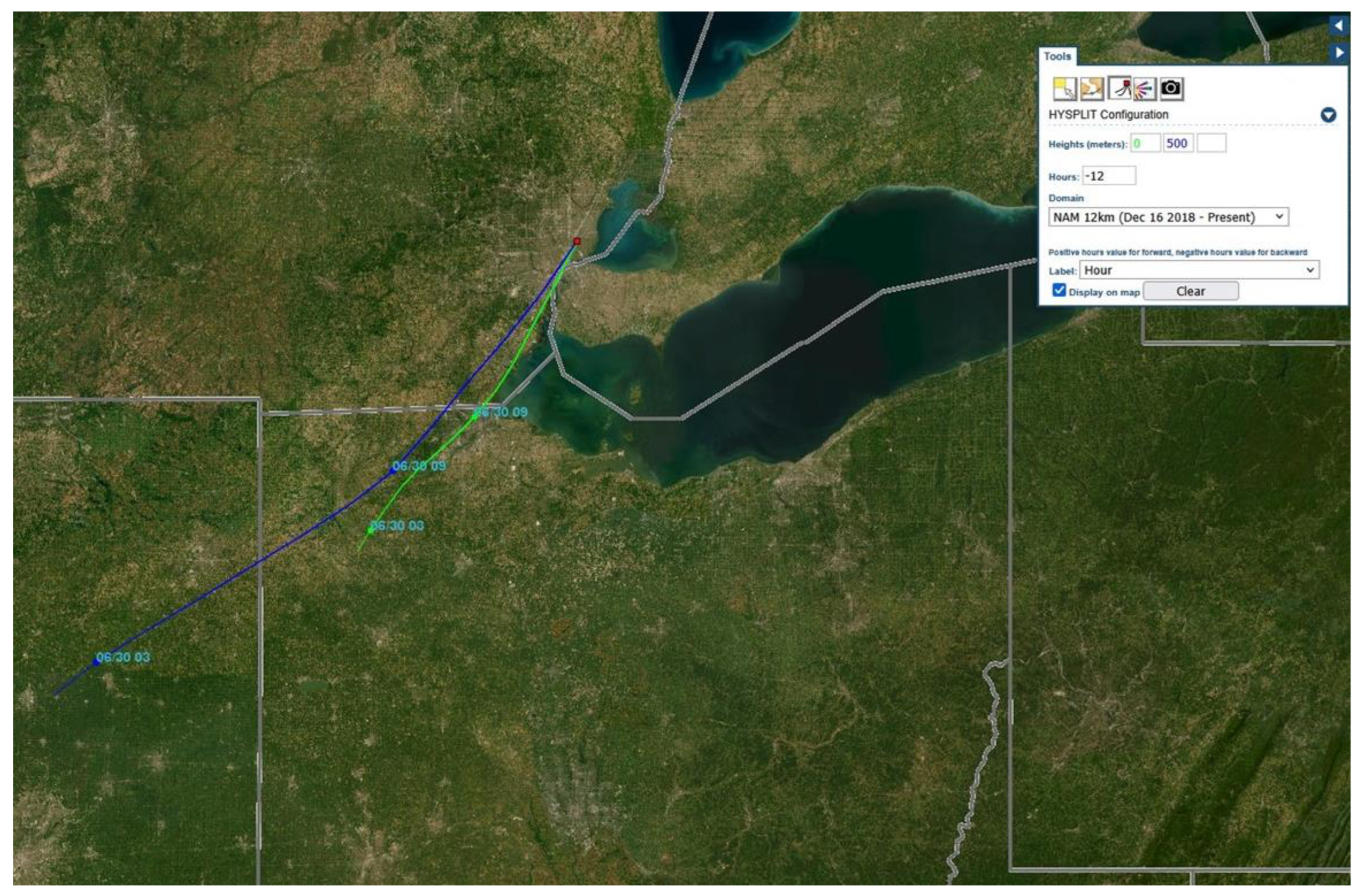
Figure 2.
A map of the area of interest in SEMI showing the locations of EGLE monitoring stations, including Allen Park and East 7 Mile Rd where ozone is monitored (blue pins).
Figure 2.
A map of the area of interest in SEMI showing the locations of EGLE monitoring stations, including Allen Park and East 7 Mile Rd where ozone is monitored (blue pins).
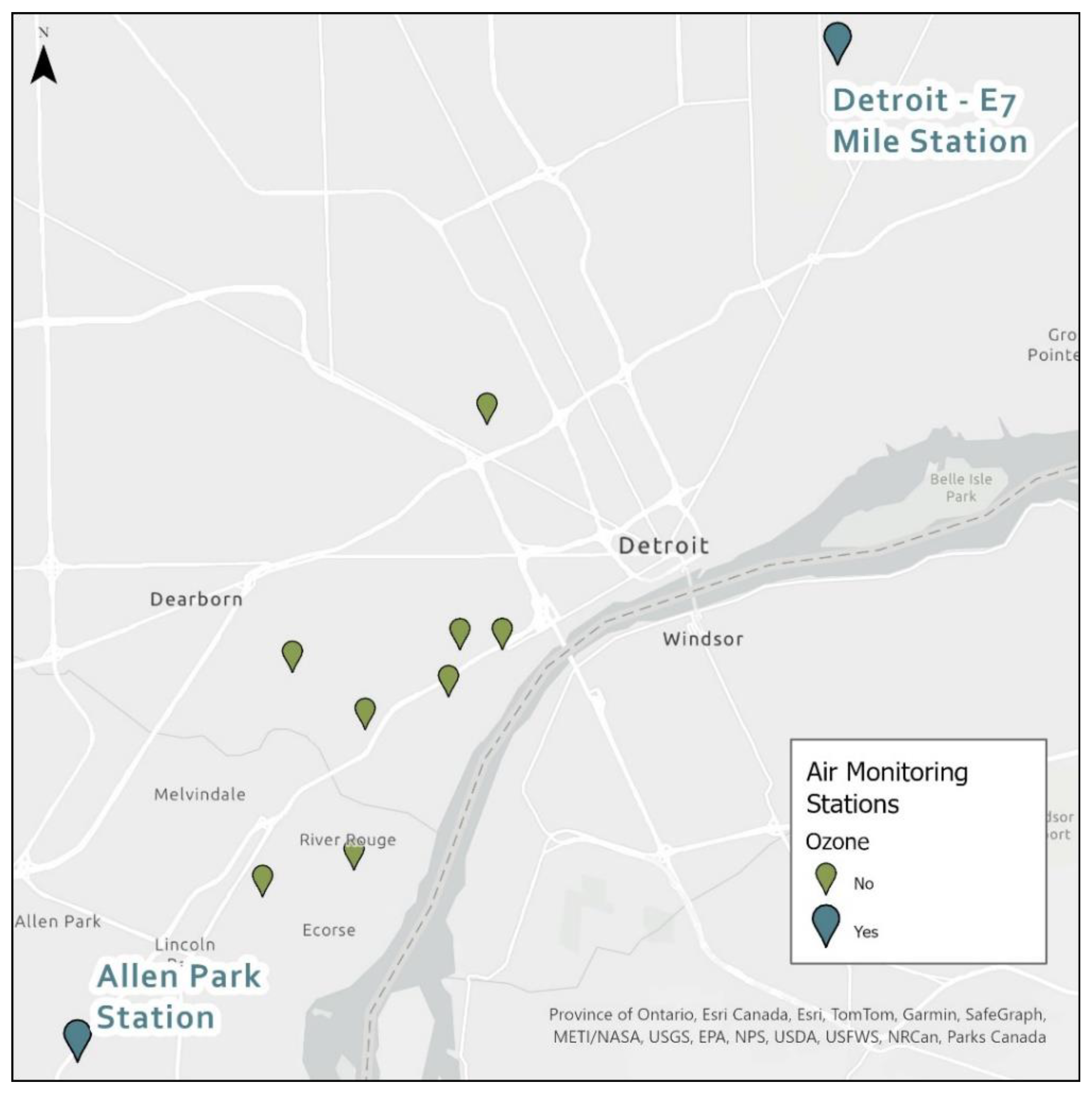
Figure 3.
The model horizontal grid used in this study with O3 contours simulated for 14:00 LST, 30 June 2022. Red label indicates East 7 Mile Rd station. Black labels indicate some major emission sources (see text above). Allen Park station is immediately to the southwest of the grid origin.
Figure 3.
The model horizontal grid used in this study with O3 contours simulated for 14:00 LST, 30 June 2022. Red label indicates East 7 Mile Rd station. Black labels indicate some major emission sources (see text above). Allen Park station is immediately to the southwest of the grid origin.
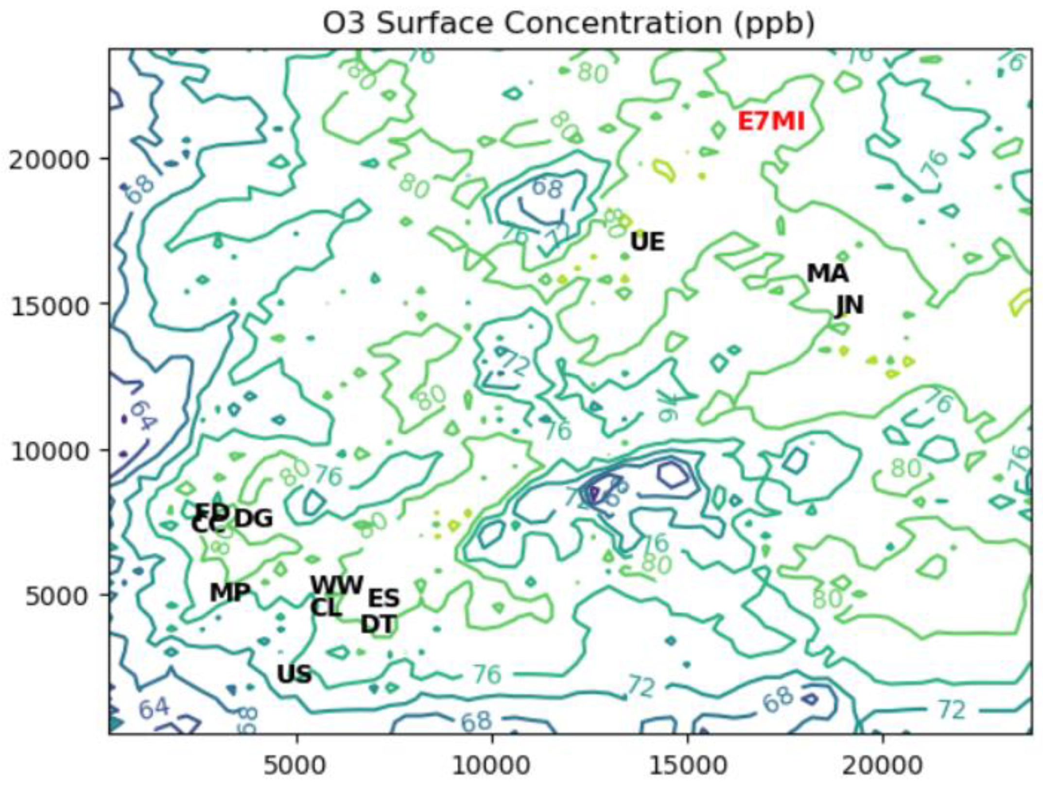
Figure 4.
Streamlines at 1 m above ground level generated by the QUIC model for 14:00 LST, 30 June 2022. The urban canopy is shown in blue.
Figure 4.
Streamlines at 1 m above ground level generated by the QUIC model for 14:00 LST, 30 June 2022. The urban canopy is shown in blue.
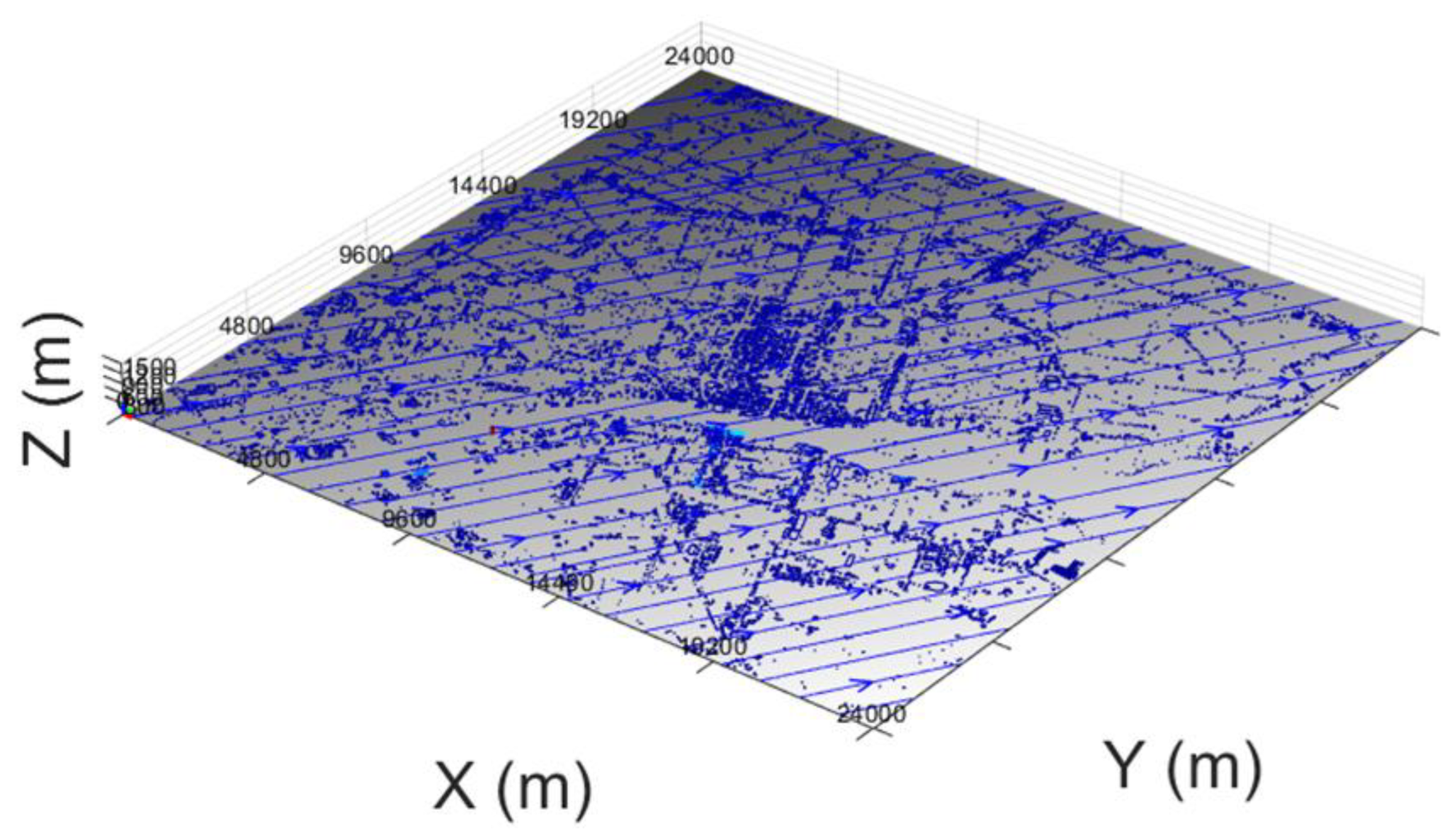
Figure 5.
Simulated O3 boundary condition (left) and vertical diffusivity profile (right) at 14:00 LST on 30 June 2022.
Figure 5.
Simulated O3 boundary condition (left) and vertical diffusivity profile (right) at 14:00 LST on 30 June 2022.
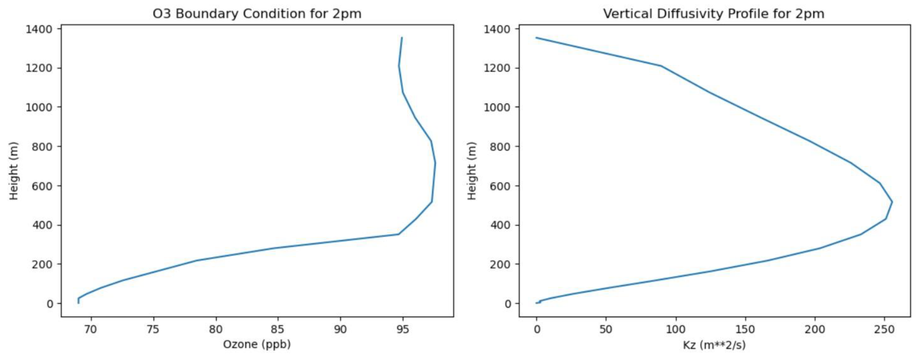
Table 1.
Comparison of modeled and measured 8-h O3 concentrations for the base case simulation.
| 8-h O3 | 9:00 – 17:00 LST | 10:00 – 18:00 LST | 11:00 – 19:00 LST |
| Modeled | 78.4 ppb | 77.9 ppb | 74.3 ppb |
| Observed | 73.0 ppb | 75.3 ppb | 76.2 ppb |
| NMB | 7.3% | 3.4% | –2.4% |
Table 2.
Comparison of modeled and measured 10-h average species concentrations for the base case simulation.
Table 2.
Comparison of modeled and measured 10-h average species concentrations for the base case simulation.
| Species |
Modeled 9:00 – 19:00 LST |
Observed 9:00 – 19:00 LST |
NMB 9:00 – 19:00 LST |
| NO | 2.4 ppb | 0.3 ppb | 668% |
| NO2 | 10.1 ppb | 2.9 ppb | 253% |
| O3 | 73.8 ppb | 73.8 ppb | –0.08% |
| Ox | 83.9 ppb | 76.7 ppb | –9.4% |
| NOy | 15.7 ppb | 5.3 ppb | –197% |
Table 3.
Comparison of ozone results between the base case and the sensitivity experiment.
| Experiment |
O3 9:00 – 19:00 LST |
Ox 9:00 – 19:00 LST |
OPE 9:00 – 19:00 LST |
| Base Case | 73.8 ppb | 83.9 ppb | 3.2 |
| No O3 Layers Aloft | 61.2 ppb | 73.8 ppb | 1.8 |
| Relative Difference | –17% | –12% | –44% |
Table 4.
Impacts of hypothetical stationary source emission reductions on MDA8 O3.
| Experiment | MDA8 O3 |
| Base Case | 78.4 ppb |
| 10% NOx Reduction | 80.5 ppb |
| 10% VOC Reduction | 78.2 ppb |
| 50% VOC Reduction | 78.0 ppb |
Disclaimer/Publisher’s Note: The statements, opinions and data contained in all publications are solely those of the individual author(s) and contributor(s) and not of MDPI and/or the editor(s). MDPI and/or the editor(s) disclaim responsibility for any injury to people or property resulting from any ideas, methods, instructions or products referred to in the content. |
© 2026 by the authors. Licensee MDPI, Basel, Switzerland. This article is an open access article distributed under the terms and conditions of the Creative Commons Attribution (CC BY) license (http://creativecommons.org/licenses/by/4.0/).
Copyright: This open access article is published under a Creative Commons CC BY 4.0 license, which permit the free download, distribution, and reuse, provided that the author and preprint are cited in any reuse.


