
Submitted:
25 July 2024
Posted:
30 July 2024
You are already at the latest version
Abstract
In this paper, we introduce a comprehensive solution aimed at enhancing the understanding of three-dimensional atmospheric pollutant dispersion. This innovative solution develops a generalized model that extends previous research and is applicable to all parameterization schemes of the equation, including wind speed profiles and turbulent diffusion coefficients, while incorporating the dry deposition criterion. Our methodology involves subdividing the atmospheric boundary layer into distinct sublayers, which facilitates a detailed examination of pollutant dispersion dynamics. Extensive validation with data from the Hanford experiment has demonstrated the accuracy of this solution in simulating pollutant concentrations. The results exhibit a strong correlation between projected and observed concentrations, underscoring the statistical reliability of our approach. This validation situates the statistical indices of our solution within an acceptable range, confirming its accuracy in predicting atmospheric pollutant dispersion. These findings thus establish our solution as a valid and effective method for studying complex environmental phenomena.
Keywords:
atmospheric parametrizations
; Atmospheric boundary layer
; Three-dimensional dispersion
; Turbulent dispersion
; Dry deposition
; Generalized Analytical Model
; Closed-form solution
1. Introduction
Understanding the dispersion, transport, and fate of atmospheric pollutants necessitates a thorough analysis of deposition processes. These mechanisms are essential in determining plume behavior and concentration patterns within the atmospheric boundary layer (ABL) [29]. However, Gaussian plume model estimates often fall short due to particle settling, deposition, or vertical gradients in diffusivity and wind speed [27]. The Earth’s surface acts as the primary reservoir for trace gases and particles, which transfer through wet and dry deposition pathways. Wet deposition is driven by precipitation, whereas dry deposition involves the adhesion or chemical reaction of trace gases and particles on surfaces like vegetation, soil, water bodies, and structures. Factors such as atmospheric turbulence intensity, the properties of gases and particles, and surface characteristics influence the efficiency of dry deposition [24]. In the absence of turbulence, even surfaces with high adsorptive capacity are ineffective in removing suspended materials, as the process is limited by molecular diffusion. Gravitational settling also plays a role in the dry deposition of particles, further complicating these dynamics [10]. The role of deposition processes in the dispersion of passive contaminants within the ABL is conventionally modeled using the advection-diffusion equation, as dictated by gradient transport theory, with deposition fluxes incorporated as boundary conditions at the surface [9]. To address this, a modified Gaussian model was formulated, initially presuming constant wind speed and homogeneous eddy diffusivity [13]. For enhanced applicability, eddy diffusivities were subsequently adjusted based on dispersion parameters relative to the downwind distance, and wind speed was modeled using a power-law relationship with vertical height [17]. However, this method introduces mathematical inconsistencies due to the employment of unrealistic parameterizations [26].
In this paper, we present an innovative approach aimed at improving the understanding of pollutant behavior in the atmospheric boundary layer (ABL). Our research introduces a generalized, one-of-a-kind model capable of adapting to all existing parameterization schemes. This model holistically integrates various wind speed profiles, turbulent diffusion coefficients, and dry deposition criteria, thereby offering unmatched flexibility and accuracy in the study of pollutant dispersion dynamics. Our model subdivides the atmospheric boundary layer (ABL) into distinct sub-layers, facilitating a granular examination of pollutant dispersion dynamics. Each sub-layer is parameterized with specific wind speed profiles and turbulent diffusivity coefficients, adopting their average values. This segmented approach allows for a detailed analysis of vertical and horizontal variations in atmospheric properties, thereby providing a more precise understanding of the mechanisms of pollutant transport and deposition. The key contributions of this work include the development of a generalized analytical model, the incorporation of closed-form solutions, and the meticulous validation of these models through empirical data. By addressing the intricacies of turbulent dispersion and dry deposition, our research offers a comprehensive framework that enhances the predictability and understanding of atmospheric pollutant behavior. In the course of this contribution, we have demonstrated the equivalence between two formulations of the pollutant dispersion problem in the atmospheric boundary layer. The problems () and () differ in their treatment of the source term: in (), the source term is directly integrated into the main differential equation, representing a point source, whereas in (), this term is included in the boundary conditions. The equivalence between () and () is proven using mollifiers (), smooth functions that handle the singularity of the source term [11]. The solution obtained not only generalizes but also extends previously established solutions. For a single layer and two-dimensional case, it corresponds to the solutions developed by Kumar [15] and Seinfeld [25]. In the context of multi-layer and three-dimensional scenarios, our model aligns with the solutions provided by Farhane et al. [7] and Marie et al. [19] This demonstrates the robustness and validity of our model across various parameterization conditions, confirming its applicability and accuracy in diverse atmospheric settings. The convergence of the proposed solution is demonstrated through rigorous analysis, showing that a minimal number of eigenvalues are sufficient. This efficiency offers a significant advantage over methods like the Generalized Integral Laplace Transform Technique (GILTT) [28], which often require many more eigenvalues for accuracy. Achieving convergence with fewer eigenvalues ensures both accuracy and computational efficiency, enhancing the model’s applicability in real-time atmospheric studies.
Validation against the Hanford experiment data [3] demonstrates the model’s accuracy, showing a strong correlation and minimal bias between observed and projected pollutant concentrations. This confirms the model’s reliability and statistical robustness. Compared with existing models by Marie et al.[19] and Laaouaoucha et al.[16] for cases without deposition, and Moreira et al.[21] and Kumar and Sharan [15] for cases with deposition, our model exhibits superior performance in predicting pollutant dispersion. These findings position our model as a powerful tool for investigating complex environmental phenomena, offering critical insights for both scientific research and practical applications in air quality management. To accomplish the goals of this study, the paper is organized as follows: Section 2 covers the modeling of the advection-diffusion equation. Section 3 explains the construction of the solution and the employed parameterizations. Section 4 showcases the results and provides a statistical performance analysis. Finally, Section 5 concludes the study.
2. Atmospheric Pollutant Advection-Diffusion Equation Modeling and Construction of Analytical Solutions
The advection-diffusion equation related to atmospheric pollution is fundamentally expressed as a principle of conservation of suspended particles. This statement is mathematically formalized by the following expression [31]:
where:
- : Represents the substantial derivative, capturing the rate of change in pollutant concentration from the perspective of a moving air parcel, embodying both the temporal and spatial variations due to airflow.
- : Stands for the total concentration of pollutants, which includes both the average concentration and the transient fluctuations attributable to atmospheric turbulence.
- : Denotes the total wind velocity vector represented by , where U indicates the east-west component, V the north-south component, and W the vertical component, encompassing both the average wind speed and its instantaneous fluctuations.
- : Indicates the partial derivative with respect to time, denoting how the concentration of pollutants changes at a fixed point as time progresses.
- ∇: Is the gradient operator, employed to calculate the spatial gradient of the pollutant concentration.
- : Describes the divergence of the wind velocity and pollutant concentration product, representing the net movement of pollutants carried by the wind across the spatial domain.
- S: Is the source term within the equation, quantifying the addition or removal of pollutants from the atmosphere via various processes such as industrial emissions, chemical reactions, or the deposition and uptake by terrestrial surfaces and vegetation.
Reynolds decomposition [30] is a pivotal technique for analyzing turbulent flows. It separates the total wind velocity and pollutant concentration into their average components, and c, and their fluctuating components, and , respectively. This separation is mathematically represented as
and
where the prime notation (’) indicates the fluctuating part of the quantity. By doing so, it facilitates the understanding of the complex interplay between the mean flow and the superimposed random fluctuations that characterize turbulent diffusion of contaminants in the atmosphere.
Incorporating the decomposed expressions for and , the advection-diffusion equation 1 is reformulated as:
Applying the averaging operator across the equation, the mean of the fluctuations alone cancels out, as they are, by definition, zero:
Expanding the term , we get:
After averaging, only the terms involving the averages and the term remain:
Assembling the mean terms and subtracting the turbulent diffusion term from the advection term , we ultimately derive the advection-diffusion equation for turbulent flow:
This equation now accurately represents the transport and spread of pollutants in a turbulent atmosphere, accounting for the mean motion of the air as well as the chaotic eddies that enhance diffusion.
In atmospheric modeling, the fluctuating wind component, denoted as , captures the erratic behavior of air movement. The gradient transport hypothesis, also known as K-theory, elucidates the mechanism by which turbulence drives materials against their concentration gradients. This is mathematically expressed by :
where the eddy diffusivity matrix , defined as , incorporates the eddy diffusivity coefficients , , and for the x-, y-, and z-directions, respectively. This setup enriches our understanding of turbulent diffusion and its impact on the spatial distribution of pollutants.
Furthermore, the equation accurately models turbulent fluxes, underscoring the model’s effectiveness in simulating atmospheric pollutant transport and distribution, and highlights the pivotal role of turbulent diffusion as described by Fick’s laws.:
Integrating Equation 2 with the mass continuity principle yields the advection-diffusion equation 1, as rigorously documented by [31]:
In physics and engineering disciplines, the concept of point forces—actions highly localized in both space and time—is a recurrent theme. To mathematically model such phenomena, the Dirac delta distribution is utilized, enabling the precise identification of point sources. For instance, a point source emitting pollutants at a continuous rate Q at a specific location is represented by the source term , formulated as:
with ⊗ symbolizing the tensor product.
To accurately model the transport of the emitted pollutants, the following boundary conditions are considered:
- (i)
- The apex of the mixing or inversion layer functions as an impervious boundary preventing the diffusion of contaminants. Consequently, a reflective flux boundary condition is postulated at the height of the inversion layer, articulated mathematically as:
- (ii)
- Addressing the scenario where a pollutant is partially absorbed by the ground surface, Calder [2] delineates an applicable boundary condition in flux terms. It is posited that the ground surface may facilitate partial removal or absorption of the pollutant via deposition, characterized by a deposition velocity :where represents the surface roughness length.
- (iii)
- The lateral diffusive flux diminishes with increasing distance from the source, approaching zero as y extends towards the lateral boundary , formalized by:
Within the context of this article, key assumptions include:
- The system reaches a state of equilibrium dispersion ();
- Contributions from and are omitted, given that the x-axis aligns with the mean wind direction, rendering the w and v components of wind velocity minor;
- Turbulent diffusion along the mean wind direction is disregarded in comparison to advective transport, implying:
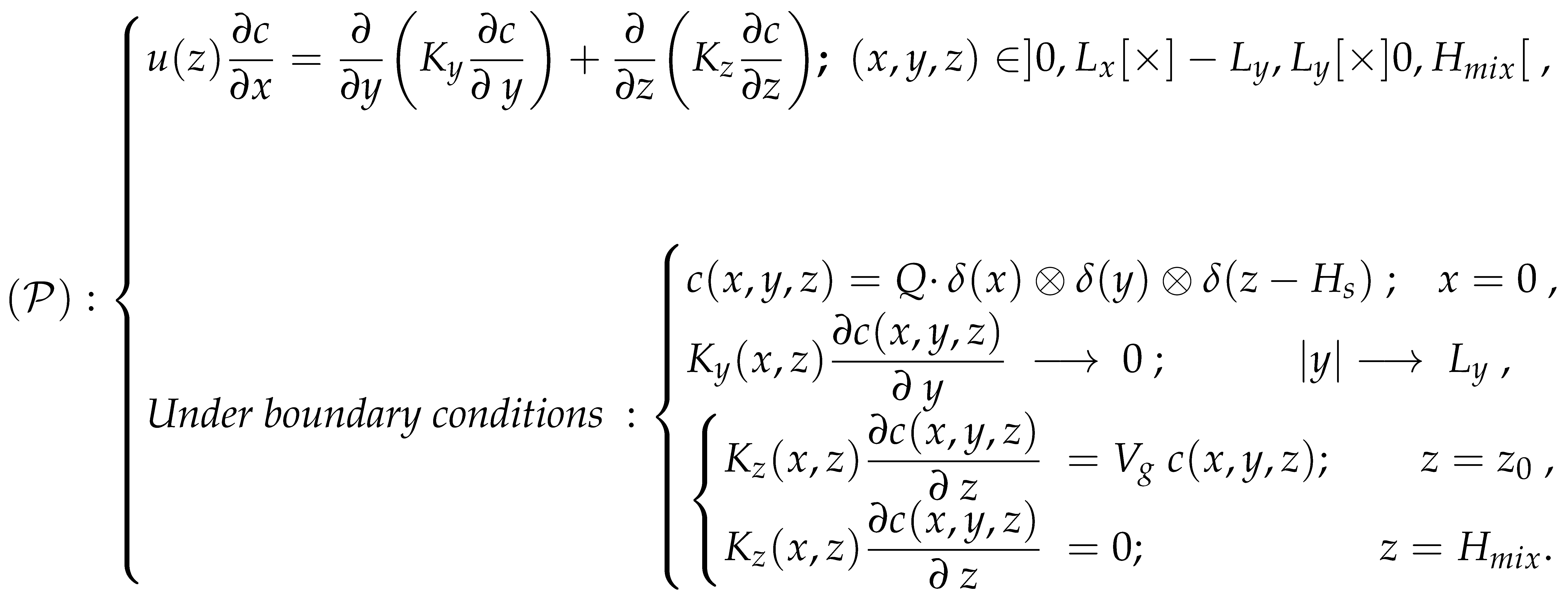
These assumptions lead to the steady-state advection-diffusion equation as follows:
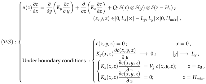
Theorem 1.
The problem is equivalent to the problem defined by:
Proof of Theorem 1.
The steps for establishing equivalence are outlined as follows:
-
Consider as the solution for of the system , and define as follows:We will establish that satisfies the requirements of system .
- To improve solution regularity, we apply mollifiers , as referenced in [11], over , defined as follows:with and using the Heaviside function , which is 1 for and 0 otherwise, where * denotes convolution.
- We differentiate with respect to x, leading to:
-
Integrating the advection and diffusion terms, we find:This confirms that corresponds to the system when n approaches infinity, thus completing the proof of equivalence between the systems and .
□
The problem can be transformed into a series of specific advection-diffusion problems defined for each sub-layer of the atmospheric boundary layer, subdivided into levels. For each level, the formulations of the turbulent diffusivity coefficients and wind profile adopt average values, as cited in [6]. Furthermore, two boundary conditions are applied at the ABL’s extremities, at and at (the height of the ABL), supplemented by continuity conditions for both the concentration and its flux at the interfaces between sub-layers. These continuity conditions, as shown in Figure 1, are expressed mathematically as follows
- The concentration at the end of a sub-layer must equal the concentration at the beginning of the subsequent sub-layer to ensure the continuity of concentration across sub-layer interfaces, as denoted by the equation
- The concentration flux, which is the product of diffusivity () and the concentration gradient with respect to the vertical axis (z), must also be continuous across the interfaces between sub-layers. This continuity is captured by the equation
We consider the atmospheric boundary layer’s intricate dynamics, where the eddy diffusivities adopt separable formulations that illuminate the interplay between horizontal and vertical mixing processes [7]. Specifically, these formulations are expressed as:
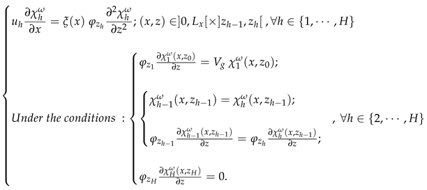
With this foundation, the equation outlines the advection-diffusion dynamics across each sub-layer of the atmospheric boundary layer, represented through a set of partial differential equations, expressed as follows:
Theorem 2.
(Solution to theProblem)
The concentration within the sub-layer, denoted by , which is the solution to the problem , is given by the following expression:
where
with :
- The coefficient is determined by the following relationship:
- The coefficient is determined by the following relationship:
- The norm is defined as:
- The parameter is characterized by the equation:with the associated eigenvalues the eigenvalues , for , associated with this problem are real and discrete. Additionally, the corresponding eigenfunctions are mutually orthogonal.
Lemma 1.
(TransformedProblem Formulation)
The problem, when the Fourier transform is applied to the lateral coordinate y, is reformulated in terms of the transformed variable , leading to the subsequent system :
 where is defined as:
and denotes the Fourier transformation of with respect to y, which is given by:
Proof of Lemma 1.
In proving the lemma, we adhere to the following steps:
- We begin by applying the Fourier transform with respect to the lateral coordinate y, as presented in Eqt 16, to the problem. The resulting equation is:
- We calculate the derivative of with respect to x, obtaining:
- We multiply both sides of Eqt 17 by the exponential term . Given that and remain constants within each sub-layer, it simplifies to:
- We apply the same method to the boundary conditions, expressing them in terms of to ensure consistency with the transformed system.
□
Having established the lemma, we now proceed to employ its results to demonstrate the theorem concerning the solution to the problem.
Proof of Theorem 2.
The construction of the solution for the problem unfolds through the following steps:
- Applying the lemma 1, we transform the problem into a formulation that depends on ;
- Representing as a series, we express it in a separated variables form:
- Verifying that the functions and satisfy their respective differential equations. We must therefore confirm that satisfies the equationand adheres to the system
- Determining the specific forms of and ensures that they are respectively expressed as:where is an arbitrary function depending on , andwhere is expressed in Eqt 14. This formulation must meet the system’s criteria, resulting in the determination of and , as specified in Eqts 11 and 12 respectively.
-
The continuity condition between sub-layers necessitates a recursion of eigenvalues and the eigenfunctions , for . This process begins by determining the eigenvalues associated with the first layer, , using the conditions related to . The resulting expressions are enumerated below:
- -
- The function is expressed as:where .
- -
- The norm of is given by:
The recursive generation of eigenvalues for the intermediate and final layers depends on the known values of the previous layers, in accordance with their respective conditions. This approach makes it possible to construct the associated eigenfunctions, succinctly maintaining continuity between the layers. For further details, please refer to Appendix Section A.1. - The Sturm-Liouville theorem [1] allows for the expanded representation of as:where the eigenfunctions form a complete and mutually orthogonal set. Consequently, is detailed as above. The coefficients are determined leveraging the orthogonality of , calculated as follows:
- Applying the inverse Fourier transform to from Equation (16), and considering that the inverse transform ofis given byleads to the final expression for the solution of the problem .
□
The Crosswind-Integrated Concentration (CIC) model is a tool for analyzing the dispersion of pollutants in the atmosphere, accounting for the horizontal wind component crucial for pollutant transport. It integrates the concentration across the lateral wind direction, y, yielding a two-dimensional concentration map along the wind direction (x) and crosswind direction (z). Mathematically, the CIC, , is defined by integrating the pollutant concentration over y from to . This integration reflects the dispersal of pollutants due to the horizontal wind and assesses their impact in both windward and lateral directions.
Corollary 1.
The Crosswind-Integrated Concentration (CIC), , is equal to as follows:
Proof.
To confirm the corollary, it suffices to verify the Gaussian integral identity:
□
Corollary 2.
The solution for the problem encompasses and generalizes the previously established solutions under specific parameterizations:
-
Single-Layer and Two-Dimensional Solution:
-
Multi-Layer and Three-Dimensional Solution:
Proof.
A detailed proof of this corollary, please refer to the AppendixB. □
Corollary 3.
In the scenario of a single-layer framework, where approaches 0 and extends to , the Crosswind-Integrated Concentration (CIC), , is defined as follows:
where:
- represents the average wind speed over the height of the mixing layer, calculated as
- denotes the average eddy diffusivity over the same height, expressed as
Proof.
To validate the Crosswind-Integrated Concentration (CIC) for a scenario where (a single-layer framework), we follow these steps:
- Substitute Single-Layer Values into the CIC Equation: Begin by inserting the conditions of a single-layer setup into the original CIC formula from Eqt (27):where .
- Apply Limits as Approaches 0 and Extends to : Evaluate the limits to reflect the shift to a single-layer framework that spans the entire mixing height :
□
Turbulent Parameters in Pollutant Dispersion Modeling
- (a)
-
Parameterizing the Wind Speed Profile,.The wind speed profile is principally derived using surface layer theory enhanced by Monin-Obukhov (M-O) similarity theory [23]. While traditionally limited to the surface layer, extending the M-O scaling across the entire Atmospheric Boundary Layer (ABL) involves maintaining a constant wind speed profile above this initial layer, ensuring the model’s extended applicability and continuity.Gryning et al. [8] have refined this approach to create a comprehensive wind speed profile applicable over the entire ABL, particularly suited for homogeneous terrain. Their advanced model employs a local mixing length composed of three component scales, leading to a robust formulation that incorporates adjustments for atmospheric stability throughout the entire ABL:where is an empirically determined constant, and , the Monin-Obukhov length [23], plays a critical role in modeling stability within the boundary layer. The mid-boundary layer length, , crucial for stable conditions, is given by:In this formulation, represents the Coriolis parameter, is the von Karman constant, and and are resistance law functions, dependent on the stability parameter . Additionally, Gryning et al. proposed an empirical formula for that enhances the model’s ability to adapt to various atmospheric stability conditions:
- (b)
-
Parameterizing the Diffusivity Profiles
- (b.1)
-
Vertical Diffusivity:In atmospheric dispersion models, the parameterization of eddy diffusivity, , significantly influences model accuracy and performance. Traditionally, has been modeled as solely a function of height above the ground, z. However, recent advancements have extended this parameterization to include the downwind distance x, recognizing its impact on near-source dispersion dynamics.An innovative approach by Mooney and Wilson [20] introduced a composite model for , blending both spatial variables into a single expression:where represents the vertical eddy diffusivity as a function of height, and denotes the along-wind length scale. This scale delineates the transition across which diffusivity reaches its extensive field value. Here, signifies the Lagrangian time scale at the source height, reflecting the turbulence’s persistence in the atmosphere.The parameterization of at the source height is given by:with representing the vertical turbulent intensity. In stable atmospheric conditions, the formulation for is:demonstrating how stability affects turbulence characteristics.Mangia et al. [18] further refined based on local similarity and statistical diffusion theories, resulting in the following relation:where represents the local Obukhov length and is expressed as:utilizing constants and , derived from the second-order closure model by Nieuwstadt [22], which accounts for stationary turbulence under a constant cooling rate.
- (b.2)
-
Horizontal Diffusivity:In the realm of atmospheric dispersion modeling, lateral eddy diffusivity plays a crucial role in determining the spread of pollutants in the crosswind direction. This diffusivity is fundamentally expressed through a relationship that ties it to the wind speed profile and the variance in lateral dispersion:where represents the standard deviation of the pollutant’s distribution in the lateral or crosswind direction, and is predominantly a function of the downwind distance x. This formulation underscores the dependency of lateral diffusivity on both the vertical wind speed profile and the rate of change in lateral dispersion as pollutants travel away from the source.This parameterization, based on the foundational work cited from Huang’s theory [12], encapsulates the dynamic interactions between wind speed and atmospheric turbulence. By integrating the vertical wind profile with the derivative of the squared standard deviation with respect to x, the model effectively captures how lateral diffusion varies with both altitude and distance from the source.
4. Results: Data Analysis and Model Validation
The Hanford experiments provided a valuable dataset to evaluate our Model of Crosswind Dispersion and Deposition Dynamics within the atmospheric boundary layer. These experiments, carried out in May and June of 1983, took place in a semi-arid region of southeastern Washington characterized by largely flat terrain. Detailed documentation of the experiments is available in the work by Doran and Horst [3]. Measurements were taken from six dual-tracer releases positioned at distances of 1100, 200, 800, 1600, and 3200 meters from the release point, under conditions ranging from moderately stable to near-neutral. Notably, the deposition velocity was only evaluated for the three farthest distances. There were six test runs in total, as summarized in the compiled Table 1. Each run had a release duration of 30 minutes, except for the fifth run, which was 22 minutes. The data collected, detailed in Doran et al. [4], were formatted as crosswind-integrated tracer concentrations.
Samplers were positioned at angular intervals of 8°, 4°, 4°, 2°, and 3° on concentric circles centered at the release point, with radii corresponding to 100, 200, 800, 1600, and 3200 meters, respectively. Crosswind-integrated concentrations offer significant advantages over individual azimuthal values, as they provide a smoother dataset by integrating over multiple samplers, thereby reducing the impact of minor variations in sampler performance. This method also mitigates issues arising from non-Gaussian crosswind tracer distributions. The terrain had a roughness length of 3 cm. The experiment involved simultaneous releases of two tracers: zinc sulfide (ZnS) as the depositing tracer and sulfur hexafluoride (SF) as the non-depositing tracer, both released from a height of 2 meters. The release points for SF and ZnS were less than 1 meter apart. Table A1 provides the micrometeorological data, including the Monin-Obukhov length (L), friction velocity (u*), and the height of the mixing layer (H). It also lists the crosswind-integrated tracer concentrations adjusted for the release rate (Q) and the computed effective deposition rates () using the surface depletion method described by Doran and Horst [3].
The ZnS tracer, being a polydisperse aerosol, presented challenges in achieving consistent size distribution estimates. This inconsistency hinders accurate prediction of ZnS deposition rates, as these depend on the mass distribution. The deposition velocity () is critical for model evaluation, but literature estimates of vary with particle size, atmospheric turbulence, and surface characteristics. Combined with uncertainties in the tracer particle size distribution, this variability complicates accurate prediction of deposition velocity. Since changes with particle size, both size distribution and deposition velocity vary with downwind distance. An effective deposition velocity () for a given distance incorporates these local variations in from the source to that distance. For comprehensive details on calculating effective deposition rates and wind velocity, refer to Doran and Horst [3].
4.1. Results and Discussions
The model was assessed by comparing the crosswind-integrated concentrations of the pollutants and at a height of meters above the ground, normalized by the emission rate Q. The comparison of predicted and observed values is illustrated in Figure 2. The vertical eddy diffusivity was parameterized according to the scheme provided in Eq. (30), while the wind profile followed the formulation described in Eq. (29).
Figure 2 presents scatter plots of predicted versus observed concentrations for the non-depositing material () (Figures (Figure 2) and (Figure 2)) and the depositing material () (Figures (Figure 2) and (Figure 2)). Data points located within the outer two dotted lines indicate agreement within a factor of 2, while the central diagonal line represents perfect agreement. It is evident that all simulated concentration data for both the non-depositing material () and the depositing material () fall within the dotted lines, indicating a good fit and suggesting that the model is more accurate when deposition processes are included. This contrast between and underscores the significant impact of deposition on model accuracy.
Figures (Figure 2) and (Figure 2) analyze the non-depositing material () using a logarithmic scale and a linear scale, respectively. The logarithmic scale emphasizes lower concentration ranges, providing a more detailed insight into the effects of deposition, while the linear scale offers a straightforward comparison across the entire concentration range. Similarly, Figures (Figure 2) and (Figure 2) present the depositing material () using both logarithmic and linear scales, demonstrating the model’s consistency and reliability in different deposition scenarios.
The results further demonstrate that increasing the discretization of the model improves the accuracy of predictions. Higher levels of discretization provide a better average representation of the vertical profiles, thereby enhancing the model’s capability to predict pollutant dispersion accurately. This improvement is particularly noticeable when comparing predicted and observed values, as the model with higher discretization shows a closer fit to empirical data.
Overall, the analysis reveals that the model performs well in simulating pollutant dispersion, particularly for scenarios involving deposition. The findings emphasize the importance of using appropriate parameterizations and the benefits of higher discretization in improving model accuracy. This comprehensive evaluation underscores the robustness of the model and its potential for reliable predictions in atmospheric pollutant dispersion studies.
Table 2 presents the performance metrics for models with and without deposition, evaluated using well-established statistical indices . These include NMSE (Normalized Mean Square Error), MRSE (Mean Relative Square Error), COR (Correlation Coefficient), FB (Fractional Bias), FS (Fractional Standard Deviation), MG (Geometric Mean Bias), VG (Geometric Variance), and FAC2 (Factor of Two). These indices provide insights into model accuracy and reliability [14].
For models without deposition (), increasing the number of discretization levels H improves performance. At , the model shows very low NMSE and MRSE, high COR, and minimal FB and FS, indicating strong correlation, minimal bias, and variability. When , performance slightly decreases but remains high, with low NMSE and high COR. At , NMSE and MRSE increase, and COR decreases slightly, but performance is still acceptable. For models with deposition (), similar trends are observed. Higher H values result in better performance, with showing high COR and low bias. The analysis indicates that all parameterizations simulate observed concentrations well, with NMSE, FB, and FS values close to zero and COR and FAC2 values close to one. Models without deposition generally perform better, but those with deposition also show good performance, particularly with higher discretization levels, demonstrating the model’s robustness and accuracy in predicting pollutant dispersion under various conditions.
Table 2 also presents comparisons between the proposed model and previous models by Marie et al. [19] and Laaouaoucha et al. [16] for , as well as Moreira et al. [21] and Kumar and Sharan [15] for . The results indicate the excellent performance of the proposed solution, as evidenced by the favorable statistical indices across various conditions and discretization levels. This demonstrates the effectiveness of the proposed model in accurately predicting pollutant dispersion, confirming its superiority and reliability.
Figure 3 illustrates the variations in downwind ground-level concentrations for various dry deposition velocities from a source height of 25 meters, as well as the influence of the number of discretizations (H) on these concentrations. The sub-figures (Figure 3), (Figure 3), and (Figure 3) correspond to , , and , respectively.
As H increases, the concentration profiles, both with and without deposition, show improved alignment with the observed data. This improvement is attributable to a more precise representation of wind speed and turbulent diffusivity profiles, thanks to higher levels of discretization. A greater number of layers allows for better capturing of the average characteristics of these profiles.
The profiles show that the highest concentrations occur for contaminants that are completely reflected from the ground. Introducing dry deposition reduces potential human exposure by decreasing airborne concentrations [5]. As dry deposition velocities increase, the location of the peak concentration moves closer to the source. This shift is more evident in the sub-figures as the depletion of pollutants becomes more significant. This behavior is consistent with the predictions obtained using the Gaussian plume model [5].
The analysis demonstrates that increasing the number of discretization layers (H) enhances the model’s performance in predicting pollutant dispersion. Higher levels of discretization result in a more accurate depiction of vertical profiles, thereby reinforcing the credibility of the model’s predictions. This finding underscores the importance of detailed vertical discretization in atmospheric modeling to achieve accurate and reliable results.
Figure 4 illustrates the numerical convergence of the proposed solution for the concentration as the number of eigenvalues increases, across different values of . The sub-figures correspond to (Figure 4) , (Figure 4) , (Figure 4) , and (Figure 4) , each evaluated at three downwind distances ( m, m, and m). This analysis demonstrates that the solution converges rapidly with the increasing number of eigenvalues.
The results confirm that the convergence behavior is consistent across different deposition velocities. The concentration values stabilize after a certain number of eigenvalues, indicating the robustness and efficiency of the proposed solution method. This quick convergence ensures that the model predictions are reliable and can be computed efficiently, even for varying environmental conditions and distances from the source.
5. Conclusion
In this study, we developed a comprehensive model for the dispersion of atmospheric pollutants within the boundary layer, incorporating various parameterizations for wind speed profiles, turbulent diffusivity, and dry deposition processes. Our approach subdivides the atmospheric boundary layer into distinct sublayers, enabling a detailed examination of pollutant dispersion dynamics. The analytical solutions obtained were validated against empirical data, demonstrating strong correlation and reliability. The results underscore the model’s robustness and accuracy, particularly with higher levels of discretization. This work not only extends existing models but also provides a framework for more precise predictions of pollutant behavior under different atmospheric conditions. Future research could focus on further refining these parameterizations and exploring their applicability in diverse environmental scenarios.
Abbreviations
The following abbreviations are used in this manuscript:
| ABL | Atmospheric Boundary Layer |
| CIC | Crosswind-Integrated Concentration |
Appendix A. Construction of the Solution Associated with the First Sub-Layer and Eigenvalue Analysis of the Problem (21).
Appendix A.1. Construction of the Solution Associated with the First Sub-Layer of the Problem (21)
The solution to Problem (21) is articulated in Eqt (23), where and are determined based on the specified conditions for . The continuity conditions establish a recursive relationship between the eigenvalues and the associated eigenfunctions for . Initially, the eigenvalues for the first sub-layer (when ) must be calculated using the associated condition for , which is
Considering the expression for as
substituting ’s expression into the boundary condition yields
where .
To satisfy this equation, we can select
which, when substituted into the expression for , yields:
Appendix A.2. Eigenvalues Analysis of the Problem (21)
In the analysis of the first sub-layer, the eigenvalues, represented by , are inferred from the norm of . Indeed:
It is paramount that the norm does not depend on any specific function form. The norm, representing a measure of magnitude or distance, should remain constant across different functions to ensure uniformity and comparability. Therefore, the eigenvalues are determined under conditions that guarantee this property, leading to:
which ultimately define the eigenvalues as
yielding a norm expression as follows:
For , the norm is specifically evaluated considering in the designated Eqt A5.
Following the complete assessment of eigenvalues for the first sub-layer, our focus shifts to the intermediate and final layers. For the intermediate layers, by implementing the specific condition
we arrive at the equation governing the eigenvalues for these layers presented as
Regarding the last layer, employing the relevant condition
leads to the formulation of the equation that yields the eigenvalues for this ultimate layer as
To facilitate a clear understanding of the eigenvalue generation process for each sub-layer, the accompanying flowchart Figure A1 concisely outlines the analytical steps involved, capturing the recursive determination of eigenvalues and the construction of eigenfunctions as discussed.
Appendix B. Derivation of Specific Solutions for
In the special case where , the eqt (9) simplifies to yield the solution as determined by Farhane et al[7]., defined by:
Were, the coefficients are as defined in eqt (26). Further analysis, with , leads to a solution analogous to that provided by Marie et al[19].
Transitioning to two dimensions and employing the CIC model, for a single layer we utilize the boundary condition at the top of the atmospheric boundary layer, specifically . This condition derives the parameters and , leading to the expression . The norm of is then given as:
matching the solution identified by Kumar [15].
For Seinfeld’s solution[25], we have:
References
- Boyce, W., DiPrima, R. & Meade, D. Elementary Differential Equations and Boundary Value Problems. (Wiley,2017).
- Calder, K. Atmospheric diffusion of particulate material, considered as a boundary value problem. Journal of Meteorology 1961, 18, 413–415. [Google Scholar] [CrossRef]
- Doran, J.C.; Horst, T.W. An evaluation of Gaussian plume-depletion models with dual-tracer field measurements. Atmospheric Environment 1985, 19, 939–951. [Google Scholar] [CrossRef]
- Doran, J.C.; Abbey, O.B.; Buck, J.W.; Glover, D.W.; Horst, T.W. Field Validation of Exposure Assessment Models. Data Environmental Science Research Laboratory, U.S. Environmental Protection Agency, Research Triangle Park, NC, EPA/600/3-84/092A, p. 177.
- Ermak, D.L. An analytical model for air pollutant transport and deposition from a point source. Atmospheric Environment (1967). 11, 231-237 (1977,1).
- Farhane, M. & Souhar, O. A Novel Development in Three-Dimensional Analytical Solutions for Air Pollution Dispersion Modeling. Environmental Sciences. 9 (2023,9).
- Farhane, M. , Alehyane, O. & Souhar, O. Three-dimensional analytical solution of the advection-diffusion equation for air pollution dispersion. ANZIAM Journal 2022, 64, 40–53. [Google Scholar]
- Gryning, S.E.; Batchvarova, E.; Brümmer, B.; Jørgensen, H.; Larsen, S. On the extension of the wind profile over homogeneous terrain beyond the surface boundary layer. Boundary-Layer Meteorology 2007, 124, 251–268. [Google Scholar] [CrossRef]
- Hanna, S.R. Applications in Air Pollution Modelling. In F. T. M. Nieuwstadt & H. van Dop (Eds.), Atmospheric Turbulence and Air Pollution Modelling. Boston: Reidel (1982).
- Hewitt, C.N. , Jackson, A. Handbook of Atmospheric Science. Blackwell Publishing. p. 633.
- Hörmander, L. The analysis of linear partial differential operators. Springer-Verlag,1990.
- Huang, C. A Theory of Dispersion in Turbulent Shear Flow. Atmospheric Environment (1967) 1979, 13, 453–463. [Google Scholar] [CrossRef]
- Irwin, J.S. A theoretical validation of the wind profile power law exponent as a function of surface roughness and stability. Atmospheric Environment 1979, 13, 191–194. [Google Scholar] [CrossRef]
- Kadyri, A., Kandoussi, K., & Souhar, O. An approach on mathematical modeling of PV module with sensitivity analysis: a case study. Journal of Computational Electronics 2022, 21, 1365–1372. [Google Scholar] [CrossRef]
- Kumar, P. & Sharan, M. A Generalized Analytical Model for Crosswind-Integrated Concentrations with Ground-Level Deposition in the Atmospheric Boundary Layer. Environmental Modeling & Assessment. 19, 487-501 (2014,12).
- Laaouaoucha, D.; Farhane, M.; Essaouini, M.; Souhar, O. Analytical Model for the Two-Dimensional Advection-Diffusion Equation with the Logarithmic Wind Profile in Unstable Conditions. Int. J. Environ. Sci. Technol. 2022, 19, 6825–6832. [Google Scholar] [CrossRef]
- Llewelyn, R.P. An analytical model for the transport, dispersion and elimination of air pollutants emitted from a point source. Atmospheric Environment 1983, 17, 249–256. [Google Scholar] [CrossRef]
- Mangia, C.; Moreira, D.M.; Schipa, I.; Degrazia, G.A.; Tirabassi, T.; Rizza, U. Evaluation of a New Eddy Diffusivity Parameterization from Turbulent Eulerian Spectra in Different Stability Conditions. Atmospheric Environment 2002, 36, 67–76. [Google Scholar] [CrossRef]
- Marie, E., Hubert, B., Patrice, E., Zarma, A. & Pierre, O. A Three-Dimensional Analytical Solution for the Study of Air Pollutant Dispersion in a Finite Layer. Boundary-Layer Meteorology. 155, 289-300 (2015,5).
- Mooney, C.J.; Wilson, J.D. Disagreements between gradient-diffusion and Lagrangian stochastic dispersion models, even for surface near the ground. Boundary-Layer Meteorology 1993, 64, 291–296. [Google Scholar] [CrossRef]
- Moreira, D.M.; Tirabassi, T.; Vilhena, M.T.; Goulart, A.G. A Multi-layer Model for Pollutant Dispersion with Dry Deposition to the Ground. Atmospheric Environment 2010, 44, 1859–1865. [Google Scholar] [CrossRef]
- Nieuwstadt, F.T.M.; van Ulden, A.P. A Numerical Study on the Vertical Dispersion of Passive Contaminants from a Continuous Source in the Atmospheric Boundary Layer. Atmospheric Environment 1978, 12, 2119–2124. [Google Scholar] [CrossRef]
- Obukhov, A. Turbulence in an Atmosphere with a Non-uniform Temperature. Boundary-Layer Meteorology 1971, 2, 7–29. [Google Scholar] [CrossRef]
- Pasquill, F. , Smith, F.B. Atmospheric Diffusion. John Wiley and Sons. p. 437.
- Seinfeld, J. Atmospheric chemistry and physics of air pollution. (1986,1), John Wiley and Sons.
- Sharan, M., Singh, M.P., & Yadav, A.K. A mathematical model for the atmospheric dispersion in low winds with eddy diffusivities as linear functions of downwind distance. Atmospheric Environment 1996, 30, 1137–1145. [Google Scholar] [CrossRef]
- Smith, R.B. A K-theory of dispersion, settling and deposition in the atmospheric surface layer. Boundary-Layer Meteorology 2008, 129, 371–393. [Google Scholar] [CrossRef]
- Tirabassi, T. Operational advanced air pollution modeling. PAGEOPH 2003, 160, 5–16. [Google Scholar] [CrossRef]
- Viúdez-Moreiras, D. Editorial for the Special Issue “Atmospheric Dispersion and Chemistry Models: Advances and Applications”. Atmosphere. 14, 1275 (2023,8).
- Visscher, A. Air Dispersion Modeling: Foundations and Applications. Wiley–Blackwell,2013,11.
- Zannetti, P. Air Pollution Modeling: Theories, Computational Methods and Available Software. Springer Science & Business Media,2013,6.
Figure 1.
Representation of the vertical subdivision of the atmospheric boundary layer into H sub-layers and the continuity of concentration and flux at the interface of each sub-layer.
Figure 1.
Representation of the vertical subdivision of the atmospheric boundary layer into H sub-layers and the continuity of concentration and flux at the interface of each sub-layer.
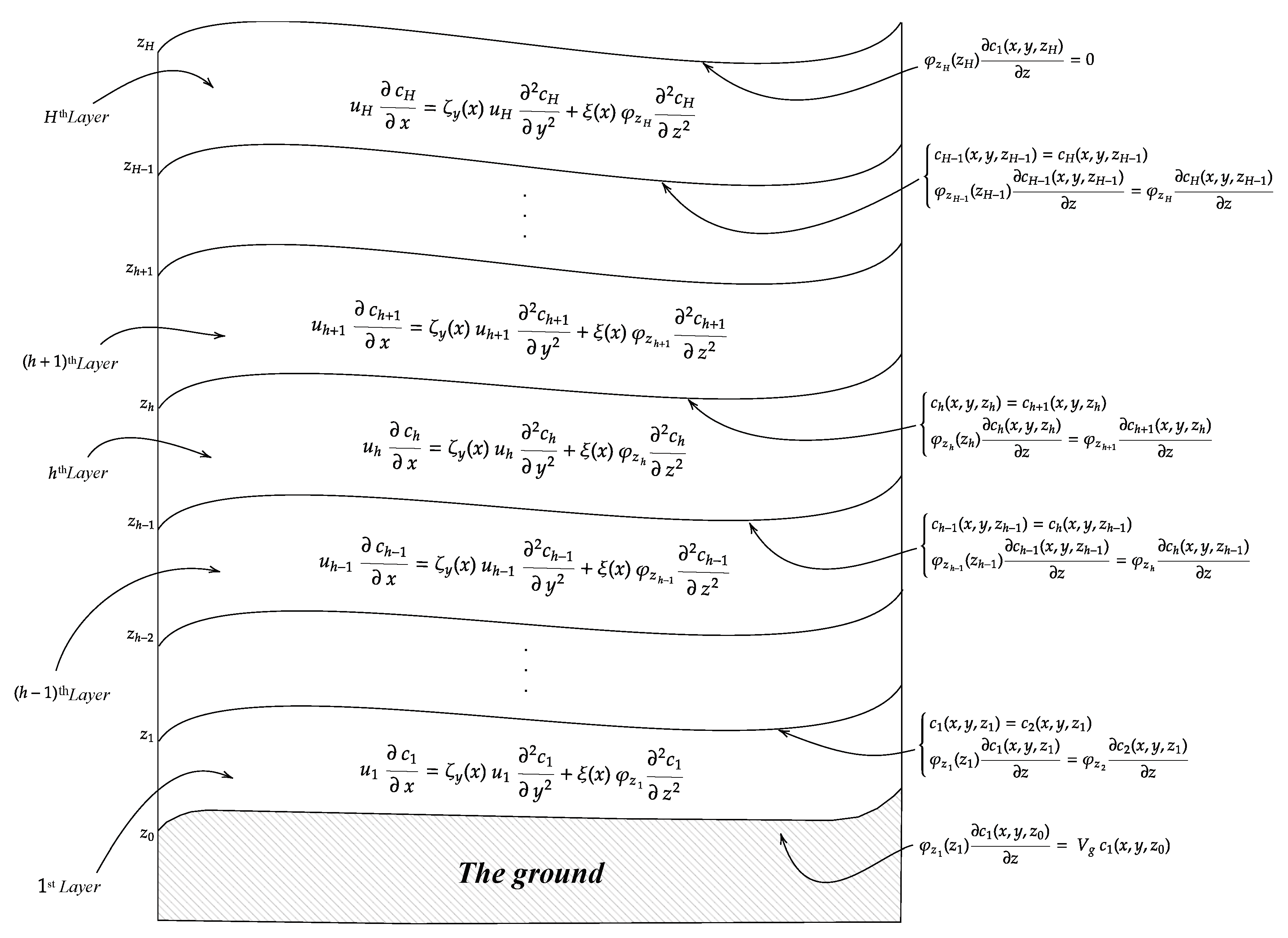
Figure 2.
Comparative analysis of predicted versus observed concentrations under different deposition conditions, illustrating model performance across a range of environmental settings.
Figure 2.
Comparative analysis of predicted versus observed concentrations under different deposition conditions, illustrating model performance across a range of environmental settings.
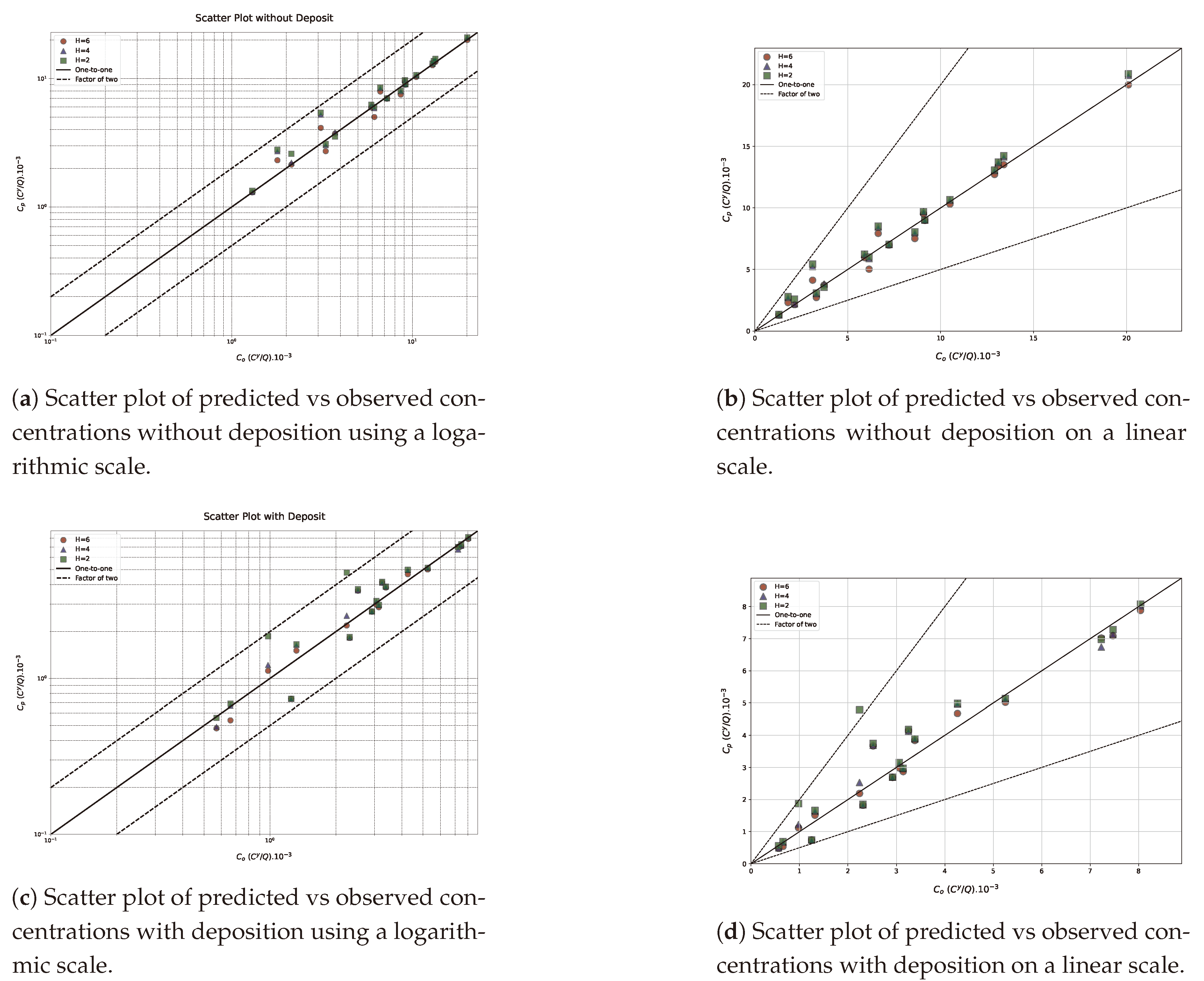
Figure 3.
Discretization of the ABL into two, four, and six sub-layers, illustrating improved adherence to model parametrizations and closer approximation to experimental measurements with increased discretization.
Figure 3.
Discretization of the ABL into two, four, and six sub-layers, illustrating improved adherence to model parametrizations and closer approximation to experimental measurements with increased discretization.
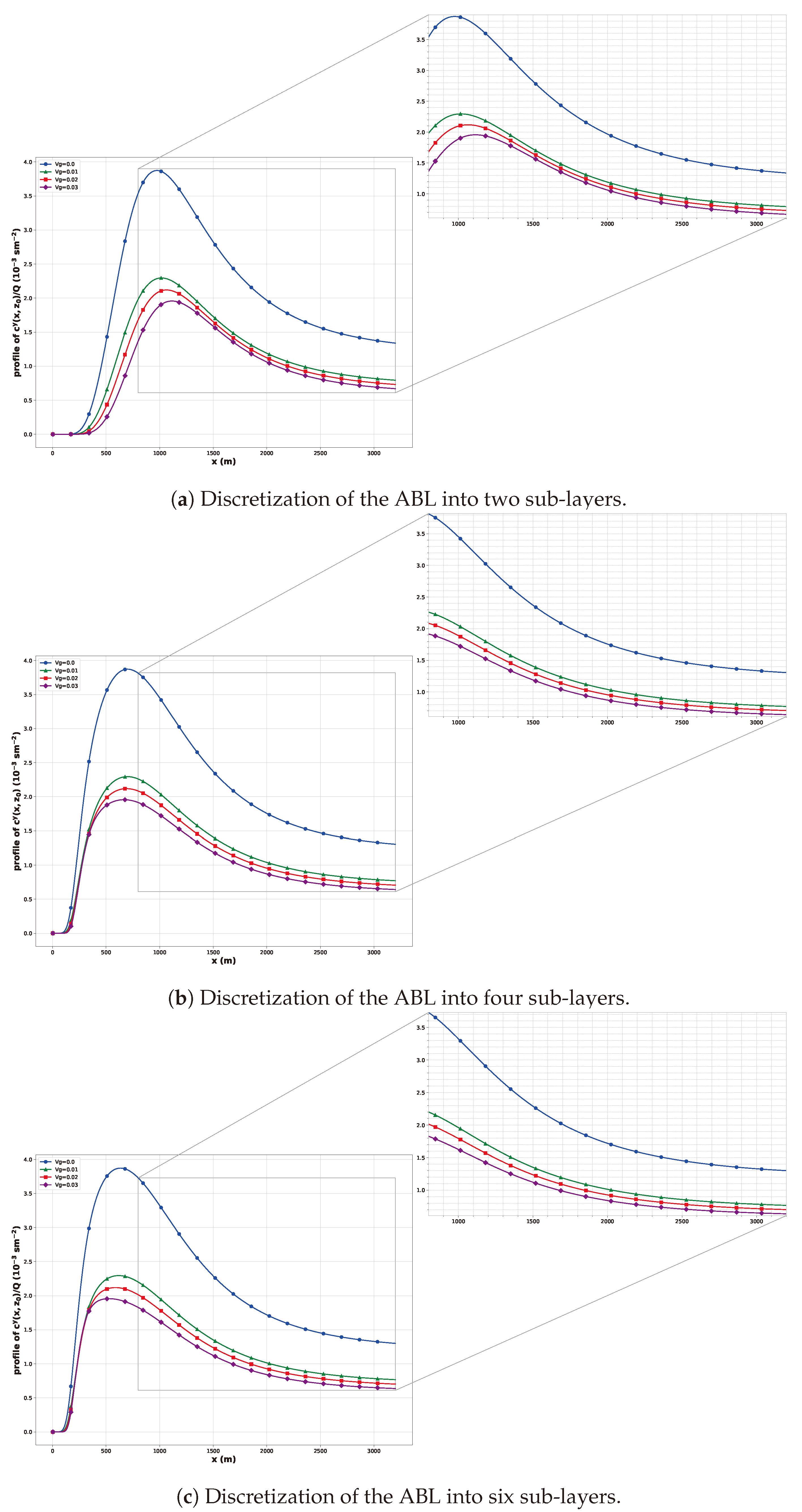
Figure 4.
Analysis of concentration convergence in a discretized ABL model across different distances from the source at cm, demonstrating the impact of varying deposition velocity .
Figure 4.
Analysis of concentration convergence in a discretized ABL model across different distances from the source at cm, demonstrating the impact of varying deposition velocity .
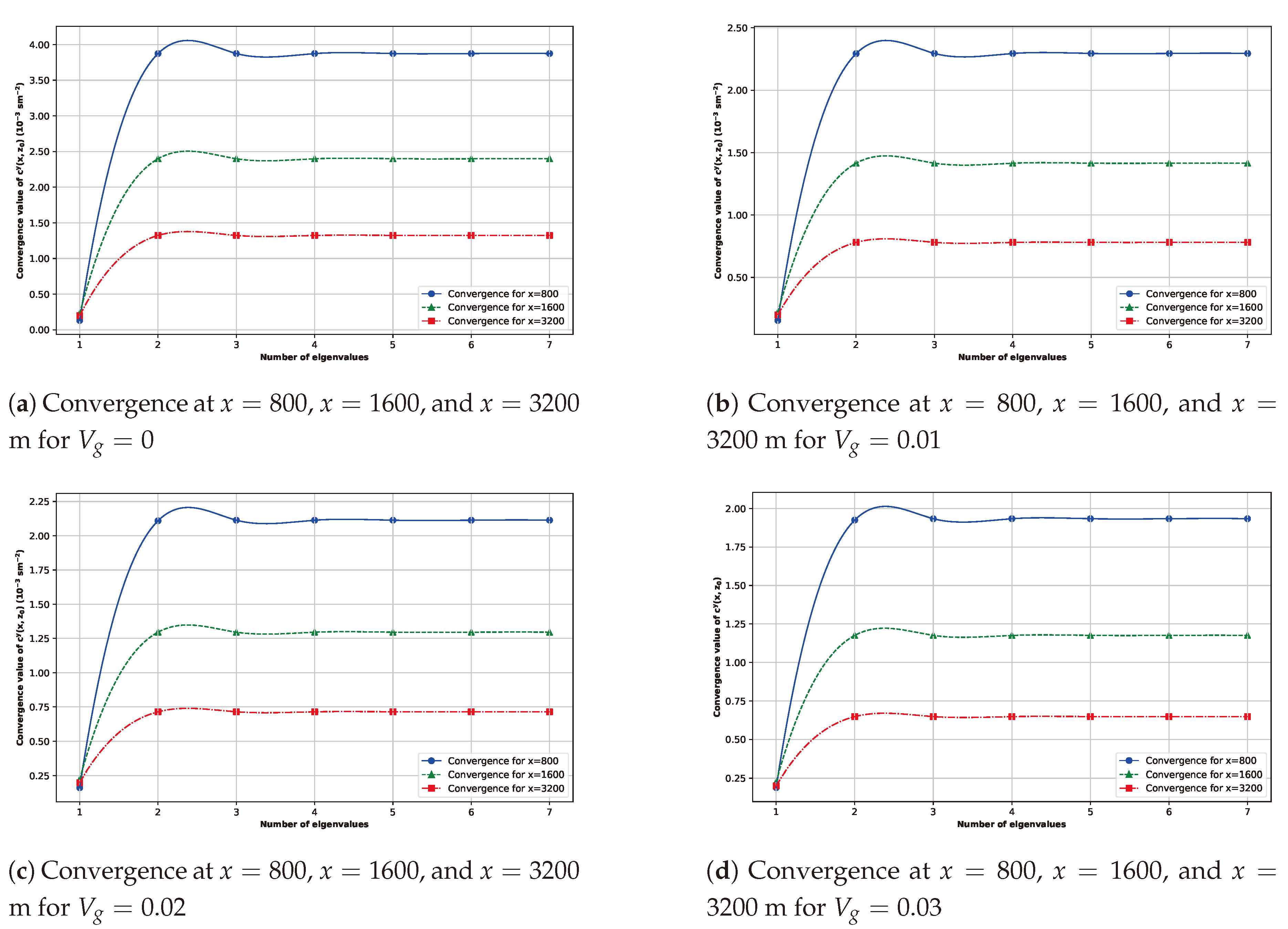
Figure A1.
Flowchart of the Process for Calculating Eigenvalues and Eigenfunctions in the Subdivided Media of the Atmospheric Boundary Layer.
Figure A1.
Flowchart of the Process for Calculating Eigenvalues and Eigenfunctions in the Subdivided Media of the Atmospheric Boundary Layer.
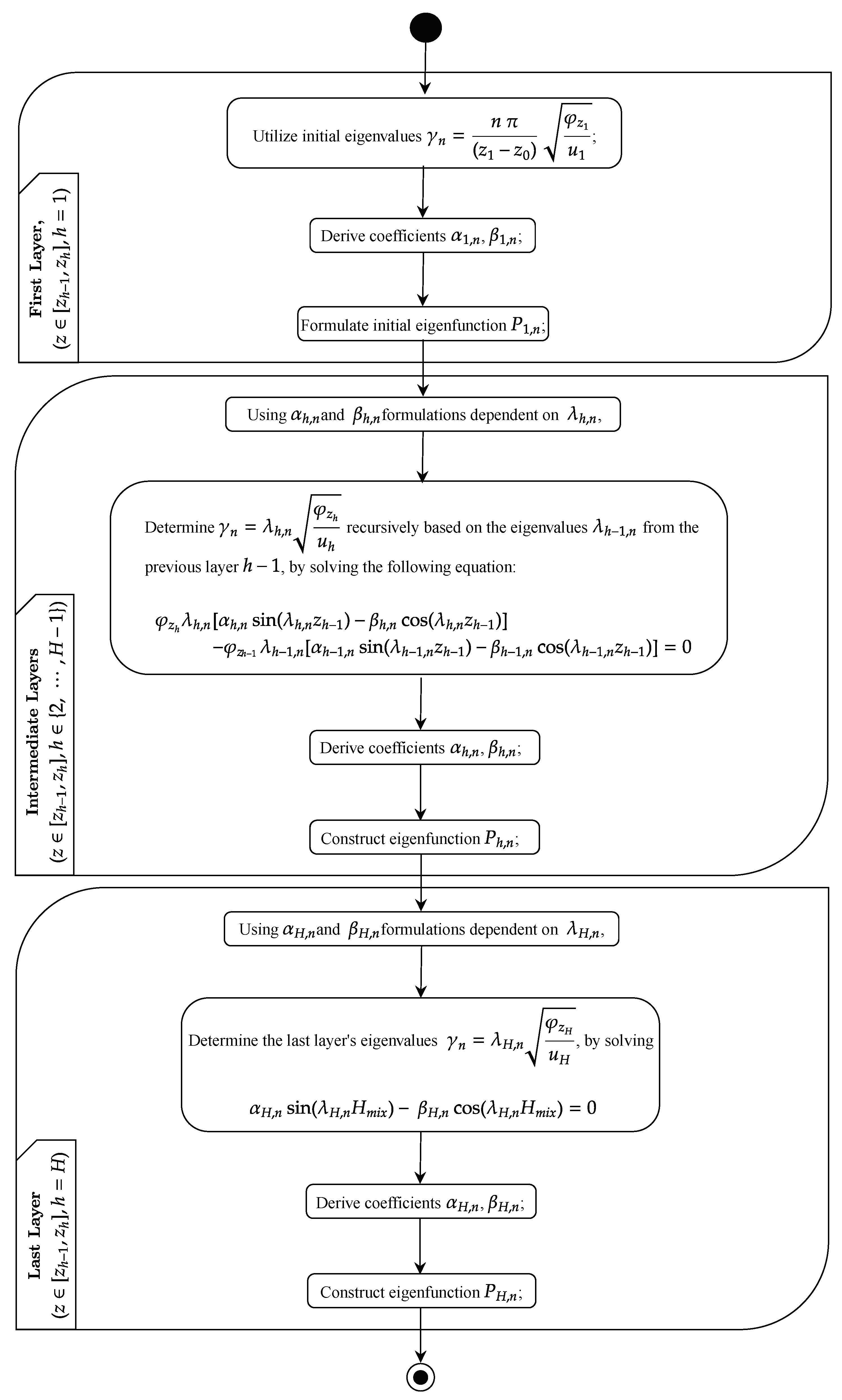

Table 1.
Micrometeorological data and observed crosswind-integrated concentrations from the Hanford diffusion experiment.
Table 1.
Micrometeorological data and observed crosswind-integrated concentrations from the Hanford diffusion experiment.
| Run | Date | Distance | ||||||
|---|---|---|---|---|---|---|---|---|
| (DD/MM/YY) | (m) | () | (m) | (m) | () | () | () | |
| 800 | 3.73 | 2.24 | 4.21 | |||||
| 1 | 18-05-83 | 165 | 0.40 | 325 | 1600 | 2.14 | 0.98 | 4.05 |
| 3200 | 1.30 | 0.57 | 3.65 | |||||
| 800 | 12.90 | 7.47 | 1.93 | |||||
| 2 | 26-05-83 | 44 | 0.26 | 135 | 1600 | 9.08 | 3.25 | 1.80 |
| 3200 | 7.22 | 2.31 | 1.74 | |||||
| 800 | 5.91 | 3.06 | 3.14 | |||||
| 3 | 05-06-83 | 77 | 0.27 | 182 | 1600 | 3.31 | 1.32 | 3.02 |
| 3200 | 1.79 | 0.66 | 2.84 | |||||
| 800 | 20.10 | 8.04 | 1.75 | |||||
| 4 | 12-06-83 | 34 | 0.20 | 104 | 1600 | 13.10 | 4.26 | 1.62 |
| 3200 | 9.15 | 3.14 | 1.31 | |||||
| 800 | 10.50 | 5.25 | 1.56 | |||||
| 5 | 24-06-83 | 59 | 0.26 | 157 | 1600 | 8.61 | 3.38 | 1.47 |
| 3200 | 6.64 | 2.92 | 1.14 | |||||
| 800 | 13.40 | 7.23 | 1.17 | |||||
| 6 | 27-06-83 | 71 | 0.30 | 185 | 1600 | 6.15 | 2.52 | 1.15 |
| 3200 | 3.11 | 1.25 | 1.10 |
Disclaimer/Publisher’s Note: The statements, opinions and data contained in all publications are solely those of the individual author(s) and contributor(s) and not of MDPI and/or the editor(s). MDPI and/or the editor(s) disclaim responsibility for any injury to people or property resulting from any ideas, methods, instructions or products referred to in the content. |
© 2024 by the authors. Licensee MDPI, Basel, Switzerland. This article is an open access article distributed under the terms and conditions of the Creative Commons Attribution (CC BY) license (http://creativecommons.org/licenses/by/4.0/).
Copyright: This open access article is published under a Creative Commons CC BY 4.0 license, which permit the free download, distribution, and reuse, provided that the author and preprint are cited in any reuse.


