
Submitted:
28 March 2025
Posted:
31 March 2025
You are already at the latest version
Abstract
The Weather Research and Forecasting (WRF) model is used to study the transport of a passive scalar plume, representing smoke from biomass burning in South America (SA). In this context, the Mellor–Yamada–Nakanishi–Niino (MYNN), Yonsei University (YSU), and Bougeault-Lacarrere (BouLac) Planetary Boundary-Layer (PBL) schemes were utilized. A total of three simulations were conducted, one for each PBL scheme, starting on August 15, 2019, and ending on August 20, 2019. This period was characterized by a high concentration of smoke, which were transported to the southern and southeastern regions of South America. During this period, the direct impact of these particulates was observed in the São Paulo Metropolitan Area (SPMA). To determine the positions of the passive tracers, data from the Fire Information for Resource Management System (FIRMS) were used to identify the regions with the highest Fire Radiative Power (FRP) during the study period. Based on this analysis, three locations in different areas were selected. To analyze the transport, synoptic fields were examined during the study period to provide a better description of the atmospheric dynamics. On the mesoscale, the impact of diffusivity was assessed for each PBL scheme. For validation, surface data from the Light Detection and Ranging (LiDAR) system, located in the São Paulo region was utilized. It was observed that one of the tracers reached the SMPA in all three simulations. However, when analyzing the other tracers, the BouLac scheme failed to transport the particulates to this region. Dynamically, the low-level jet played an active role in transporting the tracers across the southern part of domain and subsequently toward the southeastern region.
Keywords:
Fires
; Transport
; PBL
; WRF
; Passive Tracer’s
1. Introduction
Amid the ongoing rise in global population, human activities are exerting a growing influence on environmental systems, to the extent that they are altering the chemical composition of the atmosphere [1]. As highlighted by [2], aerosols and their distribution within different atmospheric layers—despite being critically important—still represent a significant area of uncertainty when examining climate change and their consequences. This uncertainty is concerning because aerosols play a pivotal role in cloud microphysics, meaning that variations in their quantity can markedly affect cloud formation. Furthermore, changes in aerosol composition can modify the optical properties of clouds, which has repercussions for precipitation patterns [3]. Estimates have indicated that human activities may have led to a 5% increase in cloud cover and a 6% increase in cloud field albedo, associated with higher aerosol concentrations in the atmosphere. One outcome is the enhanced reflectivity of clouds, driven by an elevated droplet count. This observation is consistent with findings showing that the aerosol optical depth (AOD) in the stratospheric aerosol layer—between 20 and 30 km altitude—has been rising by 4% to 10% annually since 2000 [4].
In the Southern Hemisphere, parts of South America and southern Africa are notable sources of carbonaceous aerosols generated by biomass burning, a practice that tends to occur during the austral winter [5]. In Brazil, such fires frequently take place in the “Arc of Deforestation,” often driven by the expansion of farmland and pastureland. Research indicates that ozone precursor gases released from these fires are transported by convection into the free troposphere, and then carried over the Indian Ocean by westerly winds. However, investigations into this phenomenon remain relatively sparse, underscoring the need for additional studies—particularly concerning the impact of aerosol injections into the atmosphere during fire events in South America. A notable example was observed in 2019: during the dry season,which covers the months of June to October, increased fire activity in the Amazon region facilitated smoke plume transport over a distance of more than 2,700 kilometers, eventually reaching the São Paulo Metropolitan Area (SPMA) (indicated on Figure 2) and causing daytime darkness due to high particulate concentrations. Considered one of the most populated city in Latin America, São Paulo plays a crucial role in the region’s and the country’s economy, making it essential to study the impact of meteorological events on air quality. The growing frequency of such biomass burning events highlights the urgent need to examine both the causes and the dispersal of particulate matter generated across South America. Several studies have been conducted to understand this event. [6] presented a dynamic analysis of the episode, helping clarify the synoptic circulation that led to the transport of particulates to southeastern Brazil, alongside [7], which also carried out a synoptic analysis of the event. Meanwhile, [5] offered a more quantitative approach regarding the transported aerosols, utilizing satellite like IASI and MODIS data and surface data from LiDAR and AERONET to explain the phenomenon.
With the increase in extreme events worldwide, dry periods over central South America have become increasingly frequent, contributing to the rise of fire outbreaks during winter. The European Center, through its analysis for the year 2024 using the Copernicus Atmosphere Monitoring Service (CAMS) model, indicated that a significant portion of the Brazilian states of Rondônia, Amazonas, Mato Grosso, and Acre, as well as parts of Bolivia and Paraguay, experienced more than 100 days with PM2.5 values exceeding 35 . This threshold is a critical indicator of health risks for the population during the months of September to October [8]. Furthermore, [9] presents an analysis of the 19-year growth of burned areas in the Amazon region. Due to these factors, understanding how these particulates generated by biomass burning interact and are transported through the atmosphere to other regions is of utmost importance.
To understand the impact of the atmosphere and its processes on the transport of these particulates across the region, numerical modeling is used. It is essential to validate these simulations and determine the best configuration to explain such events. One of the key parameter that can influence pollutant transport is the Planetary Boundary Layer (PBL), which is known to be directly affected by surface interactions [10]. This region can be represented by various parameterization schemes, making their evaluation crucial. In this study, we implement the "passive tracer" technique in the WRF model to evaluate their transport caused by the August 2019 fire events using different PBL schemes. The Mellor–Yamada–Nakanishi–Niino (MYNN), Yonsei University (YSU), and Bougeault-Lacarrere (BouLac) boundary layer schemes were applied across South America. To perform a comprehensive validation, we first analyze whether the passive tracers reached the São Paulo region in the simulations, using knowledge of the synoptic patterns during the event. Finally, we compare vertical profiles with LiDAR sensor data on August 18 and 19.
2. Materials and Methods
2.1. Description of Event
It is known that from June to September, referred to as the dry season, fires occur primarily in the central region of South America due to the dry weather and agricultural activities taking place there. On August 19, 2019, a high concentration of particulates from biomass burning was transported across the southeastern region, reaching the city of São Paulo. Based on previous studies, these particulates are composed of approximately 50–60% organic carbon (OC) and about 5–10% black carbon (BC) [11]. These particles served as cloud condensation nuclei (CCN) [12], aiding in the development of cloudiness over the city. Due to the high concentration of OC and the possibility of contribution to the absorption of solar radiation [13], a darkening of the sky was observed in the afternoon. Such an event can be associated with the impact of aerosols on cloud microphysics [14,15]. The synoptic analysis was conducted more thoroughly, both prior to and during the event, as reported in Appendix A.1.
2.2. Description of the Event by Smoke from GOES-16 ABI
Launched in November 2016, the GOES-16 satellite was the first in the new GOES-R ABI series to become operational. It was placed in a geostationary orbit at 75.2°W, taking the "East" position within the two-satellite constellation of the operational GOES observation system. Among the instruments onboard the GOES satellite, the "Advanced Baseline Imager" (ABI) is responsible for providing visible and infrared views of the Earth. The ABI generates images in 16 different wavelengths [16], referred to as bands and/or channels [17]. Thanks to its channels, it is possible to generate various products, such as the Fire Detection and Characterization (FDC) [18], which is based on the Wildfire Automated Biomass Burning Algorithm (WF_ABBA) and FRP-PIXEL products [19]. The FDC product contains information on the fire pixel locations, sub-pixel fire characteristics including active fire area and temperature, and fire radiative power (FRP), in addition to various data attributes including the start- and end-scan times. This product has a robust body of literature, featuring various analyses for different cases and comparisons with products from other satellites [20,21]. For our specific event, to provide a more quantitative representation of fire-affected pixels, an overlay was performed between the Cloud and Moisture Imagery (CMI) [22] and Fire/Hotspot Characterization (FHS) [23] products in true or false color compositions. Similar to synoptic analysis, the assessment was guided by daily images, focusing on the time of maximum solar incidence and, consequently, the highest likelihood of detecting fire hotspots, which in this case was set at 18:00 UTC. On the first analyzed day, August 15, fire hotspots were primarily concentrated in the northern region of Brazil,indicated in Figure 1a, while the central region remained cloud-free, reinforcing the impact of the high-pressure system observed in the synoptic analysis. Additionally, fire activity was also detected in Bolivia. The hotspots in eastern Bolivia persisted into the following day, accompanied by an increase in image opacity, indicating a rise in smoke concentration over the region and its transport toward Argentina and southern Brazil. By August 17, this transport became more pronounced as fire activity continued over Bolivia, as shown in Figure 1c. A thick layer of smoke extended across northern Brazil, Bolivia, Paraguay, and northern Argentina. On August 18, in Figure 1d, with the advance of the frontal system previously discussed, the smoke began to mix with clouds over northern Paraguay. Unlike the previous days, a shift in the smoke transport pattern was observed, now directing it toward the region of interest—São Paulo. On August 19, the day of the event in question, there was significant cloud cover over São Paulo. However, smoke transport toward the city persisted.
2.3. Model Set-Up
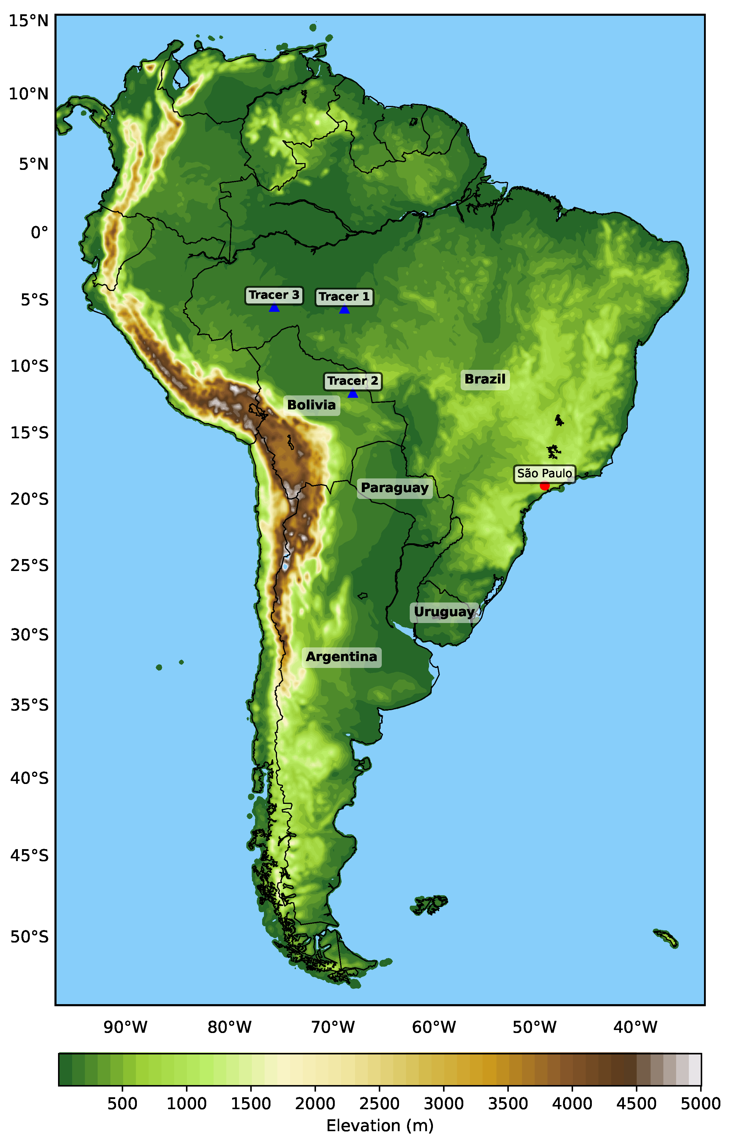
For this study, the numerical model Weather Research and Forecasting (WRF) version 4.3.3 was employed (https://www2.mmm.ucar.edu/wrf/users/download/get_source.html, last accessed: February 5, 2024). It can be described as an atmospheric numerical model developed for both research purposes (ARW–Advanced Research WRF) and operational applications (NMM–Non-hydrostatic Mesoscale Model) [24]. The model was developed through a collaborative partnership primarily among the National Center for Atmospheric Research (NCAR), the National Oceanic and Atmospheric Administration (NOAA), and various academic institutions. In this case, the ARW model is being utilized. The WRF-ARW model offers a versatile simulation framework across multiple scales, facilitating effective parallel computing. It encompasses a broad spectrum of physical parametrizations that can be adjusted to accommodate various scales and dynamic processes, where these variables interact both with the resolved scale and with each other. For this work, it was used a simulation of a single grid event with a resolution of 15 km centered on the city of São Paulo was conducted, as depicted in Figure 2, implementing 51 vertical levels. Initial and boundary data were obtained from ERA5 reanalysis fields [25] with a horizontal resolution of 0,25o× 0,25o, hourly intervals, and 37 isobaric levels.
Figure 2.
Numerical grid showing the model representation of elevation, and the location of Tracer’s starting points (blue), with the location of São Paulo (red).
Figure 2.
Numerical grid showing the model representation of elevation, and the location of Tracer’s starting points (blue), with the location of São Paulo (red).
The simulation commenced at 00 UTC on August 15, preceding the event, and ended at 00 UTC on August 20. This preliminary period was chosen due to the occurrence of fire outbreaks between August 15 and 17. Regarding the selection of parametrizations for the simulation, established and effective parametrizations, widely discussed in various international studies [26,27,28,29], were employed, thus eliminating the need for their individual analysis which are presented in Table 1.
2.4. PBL Schemes
As previously reported, this study utilizes three distinct Planetary Boundary Layer (PBL) schemes. The Mellor–Yamada Nakanishi Niino (MYNN) Level 2.5 scheme [30] is classified as a local scheme of order 1.5, employing a prognostic equation of order 2.5 to resolve Turbulent Kinetic Energy (TKE). It represents an evolution of traditional Mellor-Yamada schemes [31,32], particularly under strongly stable or nocturnal conditions. Due to its local nature, it struggles to represent large-scale transport at the top of the PBL accurately. This can be observed in cases where the use of this scheme leads to an underestimation of diffusivity representation under highly convective conditions. Similar to MYNN, the local Bougeault–Lacarrere Scheme (BouLac) scheme, developed to parameterize turbulence induced by topography in meso-beta scale models [33], employs a prognostic equation for TKE. However, it features different formulations for the production, dissipation, and diffusion terms. This scheme provides a good representation of the turbulent profile over complex surfaces while maintaining local control of diffusion, making it suitable for use under stable PBL conditions. Due to its local closure, an underestimation of mixing throughout the layer can be observed in cases of strongly convective conditions. On the other hand, Yonsei University Scheme (YSU) [34] is a non-local closure scheme based on the Medium-Range Forecast (MRF) scheme [35], with improvements in entrainment at the top of the PBL. This scheme includes a counter-gradient term that enhances the representation of convective mixing more robustly. It performs well under convective daytime conditions, as its non-local characteristic favors the representation of large eddies that transport heat, moisture, and momentum throughout the boundary layer. Consequently, it is widely used in operational forecasting and research studies. Due to its non-local representation, a tendency to overestimate the boundary layer height can be observed in some situations due to excessive vertical mixing.
Since this study aims to analyze the behavior of passive tracer transport—that is, particles that do not interact with radiation and microphysics parameterizations—it is essential to understand how each PBL scheme represents the turbulent diffusion coefficient (K) [36]. This term controls the intensity of turbulent transport of momentum, heat, and moisture throughout the boundary layer. In local schemes (MYNN and BouLac), the diffusivity term is represented by:
This formulation arises from the fact that the turbulent diffusion coefficient K directly depends on the TKE and a diagnostic mixing length, l. In these cases, diffusivity tends to be more "restricted" vertically, as each vertical level "resolves" turbulent transport based on the local TKE and stability. The diffusivity at each level is calculated solely from the variables at that level.Conversely, in the YSU scheme, diffusivity follows a non-local profile that varies with height. In a convective boundary layer, the value of K can be significantly enhanced across the entire PBL depth to represent large eddies.
These schemes are widely recognized in the academic community, with numerous sensitivity studies using the WRF model to evaluate each scheme under different conditions and events. [37] observed the efficiency of the YSU scheme in representing surface variables, with a focus on temperature and relative humidity at 2 meters. Meanwhile, [38] conducted a study to assess the impact of various PBL schemes on PM2.5 transport in the Indo-Gangetic Plain region, indicating that in this case, the MYNN scheme produced better results.
2.4.1. Model Modifications
In the present study, the introduction of three plumes originating from previously identified fire sources was conducted prior to the event day. These plumes are implemented as passive tracers, which, in the case of WRF, lack physical properties to interact with atmospheric compounds and do not influence environmental parameters. The transport of these tracers will be carried out using wind representation models in conjunction with turbulent transport occurring within the Planetary Boundary Layer (PBL). Furthermore, passive tracers in WRF are subjected to the same forcing as scalar variables present in the model, such as water vapor mixing ratio, cloud vapor mixing ratio, among others. These tracers are initially implemented as a single source in module_initialize_real.F, which contains information for initializing the tracers at the beginning of the simulation in real.exe. For continuity during the simulation, their location needs to be implemented in solve_em.F. They must be registered for the creation of output variables. The implementation was carried out based on the approach presented in [39]; however, there are numerous studies that utilize tracers to assess the propagation of particles throughout the atmosphere. For instance, [40] employs passive tracers to understand atmospheric behavior during stable periods, while [41] implements tracers to investigate pollutant propagation and dispersion in the atmosphere using high-resolution simulations. Additionally, studies such as [42,43,44] offer relevant insights employing the same technique.
2.4.2. Passive Tracer’s Position Using FIRMS Data
For the selection of the locations where the tracers would be positioned, the NASA’s Fire Information for Resource Management System (FIRMS) was used, which distributes Near Real-Time (NRT) active fire data within 3 hours of satellite observation from both the Moderate Resolution Imaging Spectroradiometer (MODIS) and the Visible Infrared Imaging Radiometer Suite (VIIRS) [45]. The NRT consists of thermal anomalies, or hot-spots, identified as a satellite passes overhead. The data is available on the FIRMS Global platform (https://firms.modaps.eosdis.nasa.gov), developed by the University of Maryland with funding from NASA Applied Sciences section to provide wildfire data to firefighters and support staff worldwide. This platform is part of NASA’s Land, Atmosphere Near real-time Capability for EOS [46]. For this work, only data from the MODIS satellite were used to identify fire hotspots for the days prior to the event in question. These data are presented in the Figure 3 below.
It can be observed that, during the first three days presented in Figure 3a–c, there was a high Fire Radiative Power (FRP) in the region of the Brazilian states of Amazonas, Rondônia, and Mato Grosso, reaching values close to 500 Megawatts (MW), which can be observed in the area inside the circle. Additionally, areas in southern Bolivia also exhibited FRP values in the range of 400-500 MW, indicating locations with intense fire hotspots. Especially in the region of Bolivia, it can be observed that during August 16, 17, and 18, the persistence of points indicating FRP above 400 suggests the maintenance of these large-scale fires. Studies such as those by [47] and [5] discussed the increase in biomass burning during August, the dry season in the central-western region of the continent. As previously observed, these fire hotspots resulted in a high concentration of particulates, which were detected in the visible channel of the GOES satellite. From this, three points corresponding to the highest concentrations during the days preceding the event were selected. The table below presents the selected points based on latitudes and longitudes.

Table 2.
Set of passive tracers based on latitudes and longitudes.
| Tracer | Latitude (o) | Longitude (o) |
|---|---|---|
| tr17_t1 | -8.851 | -61.580 |
| tr17_t2 | -15.372 | -61.617 |
| tr17_t3 | -8.096 | -66.981 |
3. Results and Discussion
3.1. Daily Transport of Tracer’s
For the analysis of the daily transport of tracers, the total column of each particulate (tr17_t1, tr17_t2, tr17_t3) was used, as it provides a more comprehensive and representative approach. For better readability, the image of the event day will be presented throughout the manuscript, while the previous days will be allocated in Appendix A.2. The total column offers an integrated view, capturing variability throughout the entire atmosphere and reducing possible distortions caused by local fluctuations. It is also worth mentioning that, to understand processes such as long-range transport, convection, and deposition, it is essential to consider all atmospheric layers. As previously mentioned, several authors have adopted this approach to better analyze atmospheric particulates, such as [48,49], among others. Upon observing the Figure A6, Figure A7, Figure A8, Figure A9 and Figure 4, it becomes evident that the three boundary layer schemes (MYNN, YSU, and BouLac) of the WRF resulted in distinct trajectories for the three tracers over the days. This highlights the fundamental role that boundary layer parameterization plays in the transport and dispersion of any mass or pollutant "plume" in the atmosphere. During the first day of the simulation, August 15 on Figure A6, it can be observed that in the MYNN simulation, the tracers initially appear concentrated near the source area, with a slight movement toward the south/southeast. Vertical mixing is still modest, as the 15th marks the beginning of the simulation. In the MYNN scheme, since the daytime turbulence is local, it does not disperse the tracer as much at higher levels. Meanwhile, the YSU scheme shows a slightly greater horizontal spreading. Transport at slightly higher layers indicates a greater sensitivity to mesoscale circulation, while the BouLac scheme presents an intermediate behavior. There is TKE generation, but with a lower entrainment potential compared to YSU; thus, the plume remains relatively compact, although there are already signs of an initial movement toward the southwest.
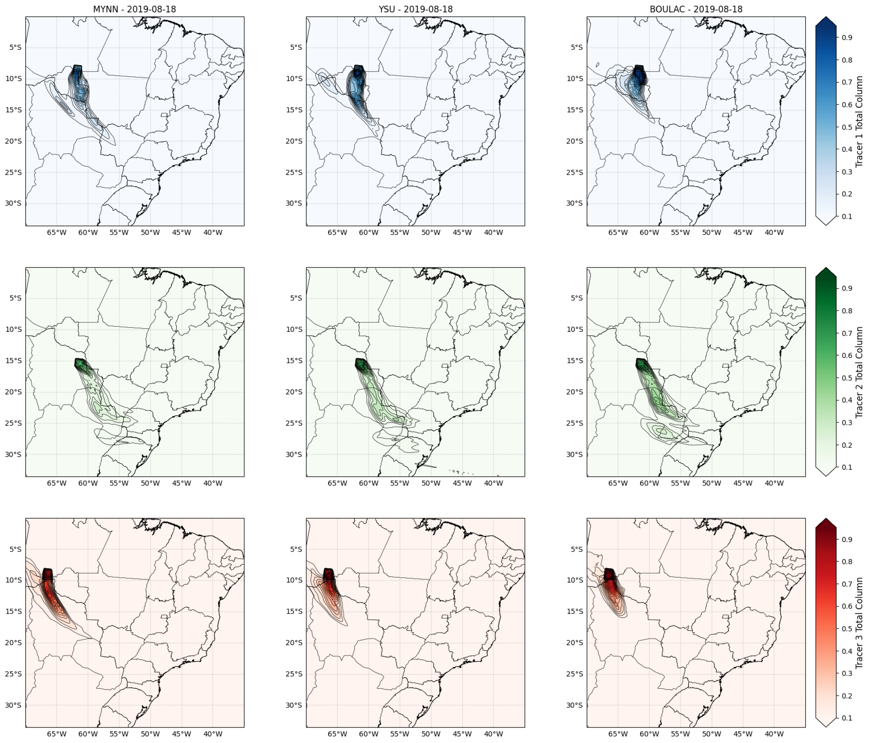
On the second day of the simulation, August 16, an "elongation" of the plume is observed in the simulation using the MYNN scheme shown on Figure A9, with the maximum concentration still confined near the source. The local diffusivity limits its extension to higher levels. The simulation with the YSU scheme continues to exhibit greater horizontal dispersion. Some studies, such as [29], indicate that this scheme can favor deeper PBLs during episodes of intense solar radiation, promoting the injection of pollutants above the surface layer. The simulation with BouLac also transports the tracers toward central Brazil, but in several areas, the plume maintains high concentrations not too far from the source. During this day, a transport corridor begins to form, and the YSU scheme tends to highlight this advancement in a more widespread manner. In contrast, MYNN and BouLac show more "concentrated" plumes, being observed in Figure A7. On August 17, for tr17_t1, the simulations exhibit similar profiles, with the YSU scheme showing greater horizontal coverage. The "tail" of the tr17_t2 plume extends from the Amazon region to areas near southern Mato Grosso. The MYNN scheme presents more restricted vertical diffusion, but the low-level flow pulls the plume. The non-local schemes, YSU and BouLac, display broader coverage over Paraguay, extending toward southern Brazil. Meanwhile, tr17_t3 remains confined near the emission source in all three simulations. The tracers tr17_t1 and tr17_t2 have already shown significant displacement toward the central region, but their arrival in the eastern belt (São Paulo) remains limited, mainly due to synoptic conditions of dry weather and predominantly northwest–south/southwest circulation. On August 18, a more consolidated shift in circulation is observed for the tracers tr17_t1 and tr17_t3, with the MYNN scheme showing the most effective horizontal dispersion in both cases. The YSU scheme, in a more intense manner, transports tr17_t1 further south, while the BouLac scheme remains more confined near the source compared to the other schemes, a pattern also observed for tr17_t3. For tr17_t2, the MYNN scheme maintains an elongated configuration, with a well-defined transport corridor. Hourly analysis indicates the arrival of these particulates in São Paulo during the day, which will be discussed later in this article. The YSU scheme stands out for its broad dispersion; in some simulations, the plume even appears at mid-levels, slightly curving southward or southeastward. The BouLac scheme generally produces results similar to MYNN, with the advantage of, in some cases, having slightly more available TKE than MYNN, allowing for deeper vertical penetration. On August 18, a more established northwest-southeast flow is observed, transporting the tracers to lower latitudes. Although penetration into São Paulo is not evident in the daily average, it is observed in the hourly analysis due to favorable synoptic conditions—specifically, the development of a frontal system over the southern region, which advances toward the southeast throughout the day being observed both in the circulation pattern shown in the synoptic basis illustrated in Figure A4.
On the day of the event, August 19, the Figure 4 indicates that tr17_t2 shows a displacement toward the southeastern region in all simulations, reaching the area where São Paulo is located. The MYNN scheme already displays an extended trajectory but remains more concentrated over central-western Brazil. The YSU and BouLac schemes exhibit the highest concentrations outside the emission source in the south region, strongly influenced by the circulation patterns discussed in the synoptic analysis, with BouLac showing greater horizontal dispersion. For tr17_t1, the MYNN scheme presents a well-defined transport corridor through the interior of Brazil, but the plume disperses or weakens before reaching São Paulo. The YSU scheme shows a higher concentration over Bolivia and western Brazil; however, it lacks the intensity and circulation support needed to disperse the plume further into southeastern Brazil, a pattern that is also observed, though less intensely, in the BouLac scheme. As for tr17_t3, the three schemes display very similar profiles, keeping the concentration confined to central Bolivia. On the fifth day of the simulation, each scheme already shows the maximum development of the transport "corridor." As will be discussed later, tr17_t2, based on hourly analysis, reaches the São Paulo region in all three simulations for the different PBL schemes. This transport across the region is primarily driven by synoptic conditions that channeled the flow—initially toward southern South America and, later, with the advance of the cold front along the coastal region, a shift in wind direction toward São Paulo can be observed, facilitating the transport of tracers into the city. As for the other tracers, based on daily data, they do not reach the region of interest due to the location of the emission source and the influence of local circulation.
3.2. Time-Height Cross-Section Comparison with LiDAR Data
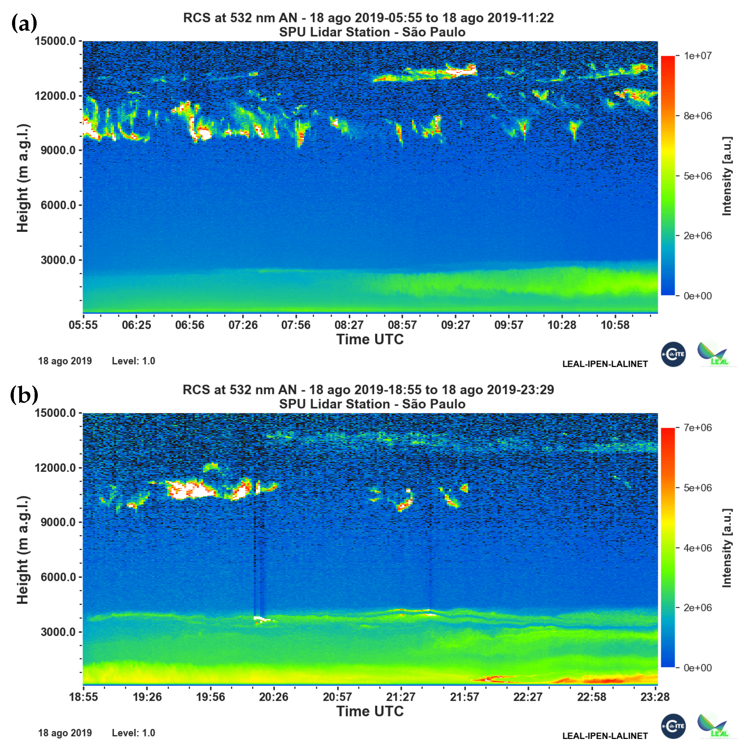
In the South American region, São Paulo (Brazil) has a multi-channel LiDAR (light detection and ranging) system, operated by the Nuclear and Energy Research Institute (IPEN). This setup is a single-wavelength backscatter system in coaxial mode, oriented vertically toward the zenith. It uses a commercial pulsed Nd:YAG laser running at the second harmonic (532 nm) with a constant repetition rate of 20 Hz. The average power can be adjusted up to 3.3 W, and the laser beam itself has a 7 mm diameter and a divergence of 0.5 mrad. The beam is directed into the atmosphere through a Newtonian telescope fitted with a 30 cm receiving mirror and a focal length of 1.3 m [50]. Studies such as those by [51] and [50] present all the technical characteristics of this fundamental instrument for the observation and analysis of particulates throughout the atmosphere. This system is part of LALINET (Latin America Lidar Network, http://lalinet.org), which is the first fully operative lidar network for aerosol research in South America. Since 2013, it has aimed to address fundamental questions about the impact of aerosols in South America through these data. During the analyzed case, data from the system are available only for August 15 and August 18, prior to the event. On August 19, the day of the event, precipitation in the municipality made it impossible to conduct measurements using the instrument. However, in this manuscript, only data from August 18 will be used for analysis, as evaluations of both the instrument data and aerosol concentration data from satellite observations indicate no occurrence of aerosols during the initial days. The combined analysis of the LiDAR profiles (RCS at 532 nm) on August 18, 2019, obtained by the SPU Lidar Station in São Paulo, generally allows the identification of two main structures along the atmospheric column. In both panels (during the morning period, 05:55–11:22 UTC, and the afternoon/evening period, 18:55–23:29 UTC), a "band" of higher intensities (with colors ranging from green to yellow) can be observed, extending from the surface up to approximately 2–3 km in height. This indicates the presence of biomass burning emissions transported to the region. The profiles reveal a well-defined aerosol layer in the lower portion of the troposphere, characteristic of urban pollution and/or smoke from wildfires, as well as mid-to-high cloud layers detected around 9–12 km.
Figure 5.
LiDAR signal time-height cross-sections at 532 nm as recorded in São Paulo on August 18, 2019, with the separation between daytime and nighttime periods. Images retrieved from the IPEN system (https://gescon.ipen.br/leal/).
Figure 5.
LiDAR signal time-height cross-sections at 532 nm as recorded in São Paulo on August 18, 2019, with the separation between daytime and nighttime periods. Images retrieved from the IPEN system (https://gescon.ipen.br/leal/).
For the analysis of tracer transport to the São Paulo region, a height-time cross-section was performed, covering the entire simulation period for the three simulations. Each image represents a different tracer. For the first tracer (tr17_t1), a signal of the tracers’ arrival is observed in the simulations using the MYNN and YSU schemes, with MYNN showing a stronger signal. This signal, indicated in Figure 6, only begins to appear on the day of the event, August 19, indicating a delay in the model relative to what was observed in the LiDAR data. Additionally, this prominent tracer signal is present at mid/high levels (around 4 km to 9 km). This suggests that the MYNN scheme is promoting (or allowing) a more intense vertical transport than would be expected solely from convection or turbulent mixing in the PBL.
When analyzing the second tracer (tr17_t2), in the Figure 7, a strong signature is observed in all three simulations, indicating that they successfully transported the particulates to the São Paulo region during the period. However, when compared to previously observed LiDAR data, it can be noted that aerosol concentration is already high on August 18, whereas in the simulations, this concentration tends to intensify only on August 19. This suggests that the model delays the arrival of these particulates. Additionally, the tracer reaches altitudes of 4 km, 6 km, and even up to 8 km or more at certain moments (depending on the scheme) within a few hours. This suggests that, at various instances, the model may be overestimating the vertical extent of the transport (or the intensity of turbulent mixing in the PBL) compared to the observed reality. Analyzing each PBL scheme separately, the MYNN scheme shows, at various moments, a high concentration of the tracer (warm colors) reaching altitudes of 6–8 km or even higher. This suggests strong vertical transport, possibly exceeding what the aerosol layer indicated by the LiDAR would suggest, as the LiDAR data show weaker backscatter signals at such high altitudes. This may indicate that the MYNN scheme is overestimating vertical diffusion or turbulence.
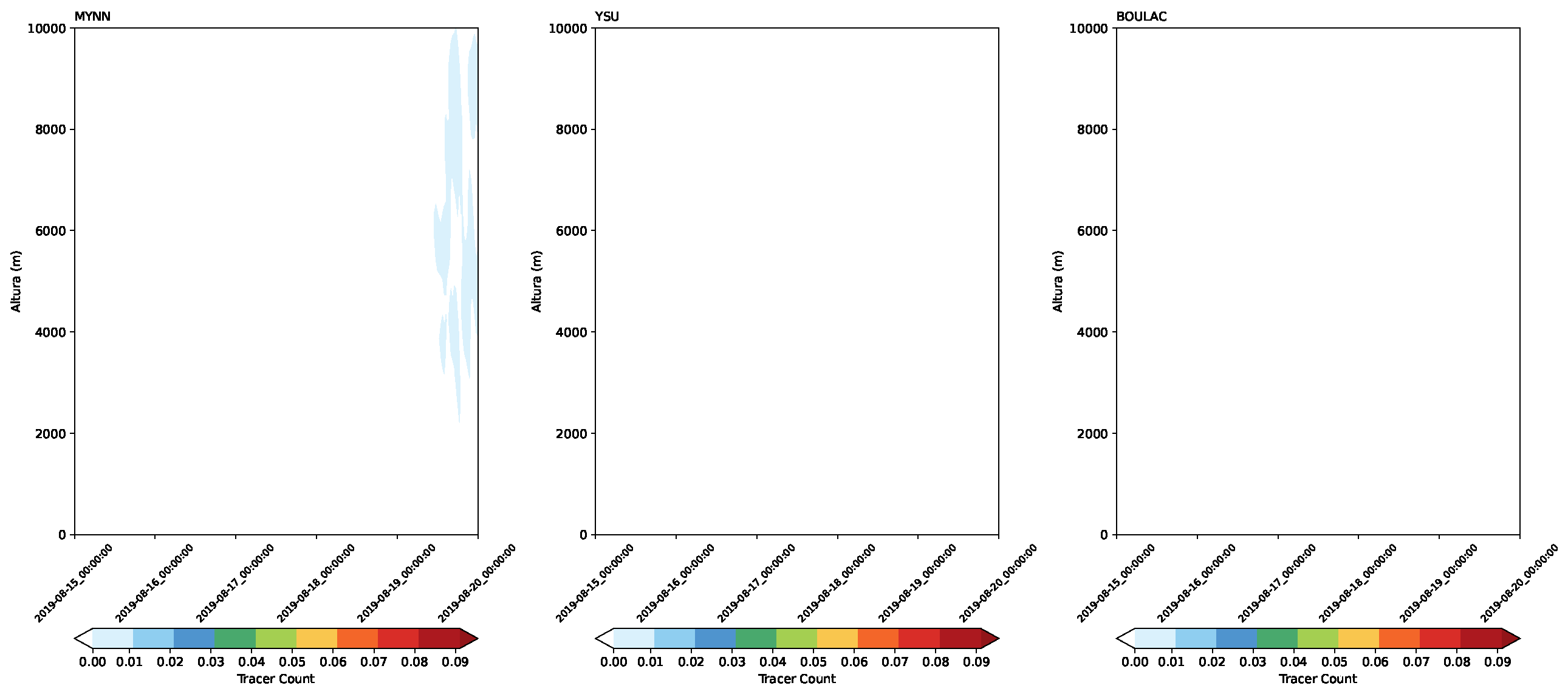
Unlike the other tracers, the third tracer (tr17_t3), in Figure 8 shows the weakest signal in terms of the amount of tracers reaching São Paulo, with the simulation using the MYNN scheme being the only one to present any signal. Once again, as observed with the other tracers, the signal appears at higher altitudes than what was seen in the LiDAR data, indicating significant vertical mixing or convective transport, carrying the tracer to much higher layers than what would typically be expected for the PBL (which, over São Paulo, usually reaches 2–3 km). On the other hand, the YSU and BouLac schemes show little to no transport to the region of interest. This underestimation of transport suggests that these schemes may not be capturing some thermally induced or convective mechanism responsible for carrying part of the pollutants to mid-level altitudes.
Overall, the simulations presented distinct representations compared to what was observed from the LiDAR data for the São Paulo region on the day prior to the event. It can be observed that all three schemes show a delay in the arrival of particulates, which only reach the region on August 19, whereas measurements already detected their presence on August 18. When analyzing each tracer separately, it is evident that the second tracer was the only one that effectively reached the region, meaning it exhibited a more evident concentration and signal. This could be explained by several factors, such as the location of the emission source or even local topography, which may have facilitated low-level transport. Another important point to highlight is that the signals of the tracers observed in São Paulo indicate that they reached altitudes above 3 km, once again diverging from the observations, where aerosol concentration was predominantly between 2–3 km. Despite the differences in PBL schemes, all of them presented a well-mixed layer, transporting the particulates above it.
4. Conclusions
In this study, we used the WRF ([24]) to describe the transport of passive tracers across the South American region as a representation of the event that occurred on August 19, 2019, when a large amount of particulates from biomass burning was observed in the region of São Paulo, Brazil, which contributed to the reflectivity of shortwave radiation, reducing solar incidence over the area during the afternoon period. Such tracers do not interact with radiation or cloud microphysics and are therefore solely influenced by dynamic circulation. Changes were made to the model code to implement tracers, whose positions were selected based on fire data extracted from the Fire Information for Resource Management System (FIRMS). Three passive tracers were set at locations with the highest fire intensity during the days preceding the event. To analyze the initial transport and the impact of the Planetary Boundary Layer (PBL) and its diffusivity, three different PBL schemes were evaluated through three simulations. The choice of schemes was based on widely used approaches in the literature, such as the local Mellor–Yamada Nakanishi Niino (MYNN) Level 2.5 scheme [30] and the non-local Yonsei University Scheme (YSU) [34]. Since the tracers are located in the Amazon region, covering Brazil, Bolivia, and Paraguay, the third scheme chosen was the Bougeault–Lacarrere Scheme (BouLac) [33], as it is commonly used in cases of more convective PBLs during the daytime period in the Amazon region. The event was described, and a synoptic analysis was conducted to understand the atmospheric conditions during the period. Since these tracers are passive, they do not interact with the model’s chemistry, radiation, or microphysics and are therefore only influenced by the dynamics. Due to this, data from the LiDAR (Light Detection and Ranging) instrument, located in the city of São Paulo, were used to observe whether the model was able to transport the tracers to the region during the simulation.
In this context, it was observed that during the first days of simulation, the transport of tracers was mainly controlled by local circulations, and, in general, they remained confined to levels close to the surface. As the simulation progressed, with the daily profile and the development of turbulence across the three schemes, the tracers began to be transported to higher levels above 3 kilometers. From a synoptic perspective, the influence of a high-pressure system over central Brazil and the wind convergence due to the development of a frontal system in the southern region favored the occurrence of a low-level jet (LLJ), which contributed to the transport towards southern regions of the emission sources on days 16 and 17. As the frontal system advanced towards southeastern Brazil, the change in wind circulation at lower levels favored transport to the region of interest, namely the city of São Paulo. When analyzing the tracers individually, it was observed that the one whose emission source was closest to the region of interest showed the strongest signal of tracer presence, specifically tr17_t2, which was expected. Additionally, an aspect that was not explicitly addressed in this manuscript but should be noted is the influence of local topography on the initial transport. As previously indicated, daytime convection and PBL influence transported the tracers to levels between 2 and 3 km. However, in the case of tr17_t3, its proximity to the beginning of the Andes Mountain range may have influenced the particulate transport.
When analyzing the influence of Planetary Boundary Layer (PBL) schemes, despite each scheme having its particularities (for example, greater vertical mixing in non-local schemes like YSU), all were capable of representing large-scale transport. However, the choice of scheme significantly impacts the intensity and timing of transport. The MYNN scheme was the only one that showed a signal for all three tracers in the region of interest, which can be explained by the fact that, at certain moments, it exhibited more intense vertical transport. This behavior caused part of the tracer to rise to higher layers. In these layers, synoptic winds were favorable for carrying the particulate matter to São Paulo, unlike what occurred with the other two parameterizations. Additionally, this scheme may have overestimated the intensity of TKE (Turbulent Kinetic Energy) under specific conditions, injecting the tracers into higher levels. As previously mentioned, topography may have influenced this transport, and how each parameterization represents this interaction was an important factor in facilitating transport. In the other parameterizations (BouLac and YSU), either the tracer remained more "trapped" at lower/middle levels without entering the high-altitude flow that would carry it to São Paulo, or it was transported in a different direction due to distinct diffusivity patterns. Nevertheless, the simulations, in general, showed a delay of about one day in the arrival of the particulates when compared to LiDAR data; furthermore, there were indications of an overestimation in the transport height.
The principal results of this study may be summarized as follows:
- Synoptic circulation was crucial in channeling particulates southward and then southeastward.
- Despite showing a delay compared to observations and the displacement of particulates to higher levels, the WRF model simulations generally provided a good representation of particulate transport across the region.
- The MYNN planetary boundary layer (PBL) scheme yielded the best results, with tr17_t2 reaching the region of interest with a significantly strong signal compared to observations.
In summary, this study highlights the importance of considering different PBL parameterizations to adequately capture both the vertical evolution and horizontal dispersion of aerosols in biomass burning scenarios. This is essential for more reliable estimates of the environmental and air quality impacts in regions far from emission sources. For future studies, it is important to use the WRF model with chemical coupling (WRF-Chem) to assess not only the transport but also the impact of these particulates on radiation schemes and cloud microphysics.
Author Contributions
Conceptualization, D.L.B., U.R. and V.A.; Investigation, U.R., D.L.B and V.A.; Methodology, D.L.B, U.R., V.A.; Software, D.L.B and U.R.; Validation, D.L.B, U.R and V.A; Formal Analysis, D.L.B, U.R., V.A, D.K.P., L.A.S., G.D.B and E.L.; Visualization D.L.B., U.R.; Writing–original draft, D.L.B, U.R. and V.A.; Writing–review & editing, L.A.S; All authors have read and agreed to the published version of the manuscript.
Data Availability Statement
All codes in this study to initiate and run the model are publicly accessible on GitHub (WRF: https://github.com/douglima8/WRF_TRACER).
Acknowledgments
We thank the CAPES (Coordination of Improvement of Higher Education Personnel) has been the supporter of the research activity (B2IST “Biomass Burning and Impacts in the Southern Tropics” registered under no. 88881.694487/2022-01 and AEROBI "AERosol Observations over Brazil and Impacts" registered under no. 88881.711960/2022-01 projects) and the National Research Council—Institute of Atmospheric Sciences and Climate of Italy. We especially thank the collaborators Eduardo Landulfo and Giovanni Souza, who are part of the Lasers and Applications Center (IPEN/CNEN-SP), for providing us with the images obtained from LiDAR data during the day of the analyzed event.
Conflicts of Interest
The authors declare that they have no known competing financial interests or personal relationships that could have appeared to influence the work reported in this paper.
Appendix A
Appendix A.1. Sypnotic Conditions During the Event
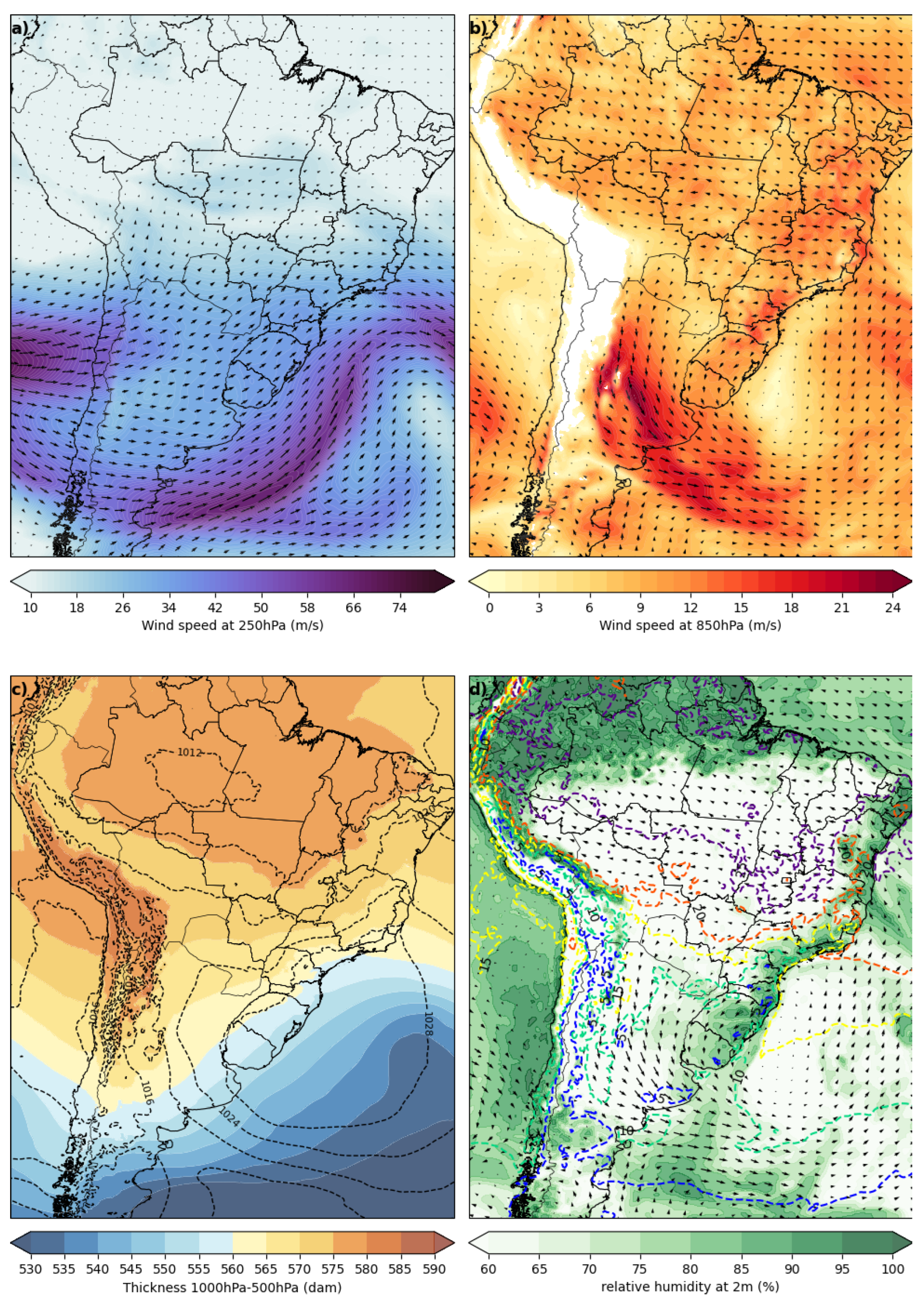
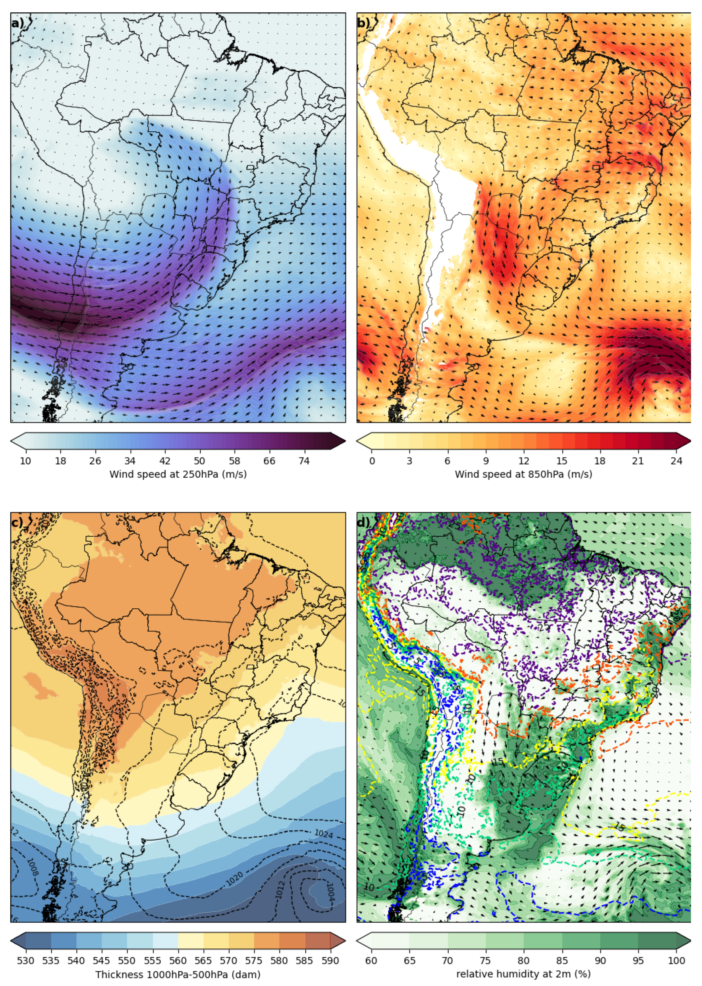
Synoptic systems typically develop over a span of a few days, making time intervals of 12 to 24 hours adequate to capture the progression of atmospheric processes on this timescale.During August 15th, the study region was directly affected by a high-pressure system with its center located over the ocean, as observed in Figure A1c. This system generated stability and calm winds over the São Paulo region. Due to several factors, such as the rotation of our high-pressure system, the Andes mountain range, and the formation of a cyclonic system to the south of South America, an increase in wind intensity near the surface was observed during the early hours of the day over northern Argentina, extending to the ocean, as indicated in Figure 1b. This more intense circulation, also known as a Low-Level Jet (LLJ) [52,53], transports considerable moisture from the Amazon to the La Plata basins. Besides the moisture transport, which can be seen in Figure A1d, this northerly flow also results in warm air advection over the southern regions of South America, covering the Brazilian state of Rio Grande do Sul, northern Argentina, and part of Paraguay. Throughout the day, this high-pressure system moves towards the ocean, altering the region of maximum wind intensity in the lower levels. However, the low-pressure system, which initially develops over the ocean early in the day, intensifies, further supporting this northward flow into the region. It is worth noting that, due to this circulation towards the southern region, this LLJ assists in the transport of particulates across the southern region, which was observed and measured at AERONET stations in the central region of the state of Rio Grande do Sul and also in the Buenos Aires region in Argentina. At upper levels, the presence of the subtropical jet (STJ), an intense and relatively narrow air current located in the upper levels of the troposphere, observed around the 200 hPa level [54], is seen over the Atlantic Ocean region. During the day, it splits into two branches, one of which extends over the southern region of South America and above the low-pressure system over the ocean, potentially contributing to its intensification. During the first day of simulation, the LLJ assists in the transport of particulates over the southern region of South America, covering Argentina, Brazil, and Uruguay; this is caused by the direct influence of synoptic systems.
Figure A1.
Synoptic fields on August 15 at 0:00 UTC from the WRF model: a) Wind field up to 250 hPa; b)Wind field up to 850 hPa; c) Surface Pressure (isolines) and thickness 500-1000 hPa field (shaded contours); d) Wind field up to 850 hPa (vectors), temperature at 2m (isotherms) and relative humidity at 2m (shaded contours).
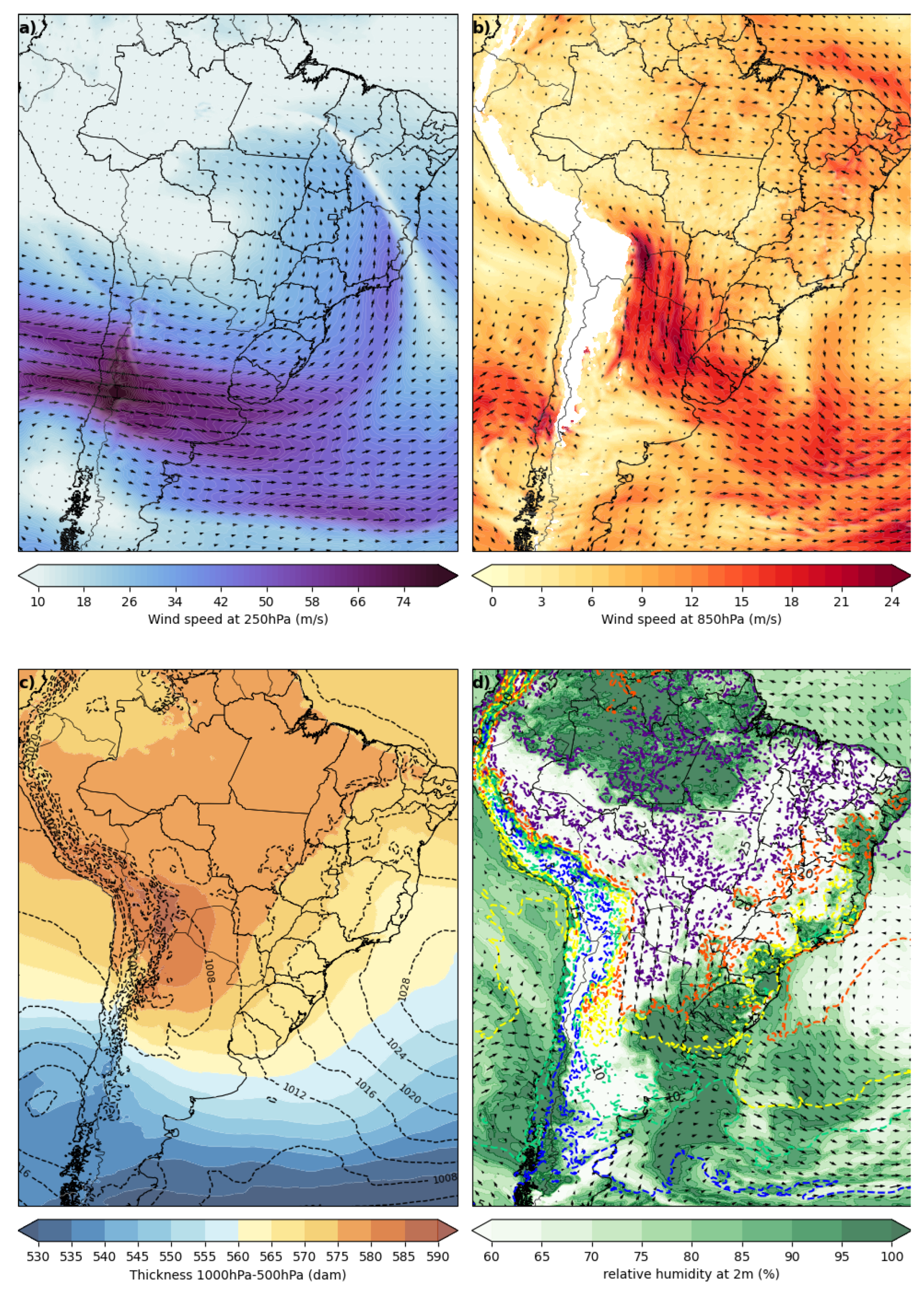
On August 16, 2019, the high-pressure system continues its movement towards the Atlantic Ocean, as seen in Figure A2c, still influencing the intensification of winds in the northern region of Argentina, as shown in Figure A2b. This system moves longitudinally, which explains the persistence of its influence over the central region. Furthermore, as previously mentioned, stability over the São Paulo region remains throughout the day. From Figure A2b–d, the intensification and displacement of the low-pressure system in the southeastern Atlantic Ocean can be observed, moving out of the domain by midday. This system contributed to wind convergence at 850 hPa near its center, along with wind convergence in the central-western region. At upper levels, an increase in the amplitude of the subtropical jet can be observed during the early hours of the day. Due to its position, this jet is often associated with the transition between tropical (warmer) and extratropical (colder) air masses, favoring the formation of a strong baroclinic gradient, which is confirmed by the thickness values shown in Figure A2c. During the second day of simulation, the transport of particulates to the southern region is maintained due to the influence of synoptic systems at lower levels.
Figure A2.
Synoptic fields on August 16 at 0:00 UTC from the WRF model: a) Wind field up to 250 hPa; b)Wind field up to 850 hPa; c) Surface Pressure (isolines) and thickness 500-1000 hPa field (shaded contours); d) Wind field up to 850 hPa (vectors), temperature at 2m (isotherms) and relative humidity at 2m (shaded contours).
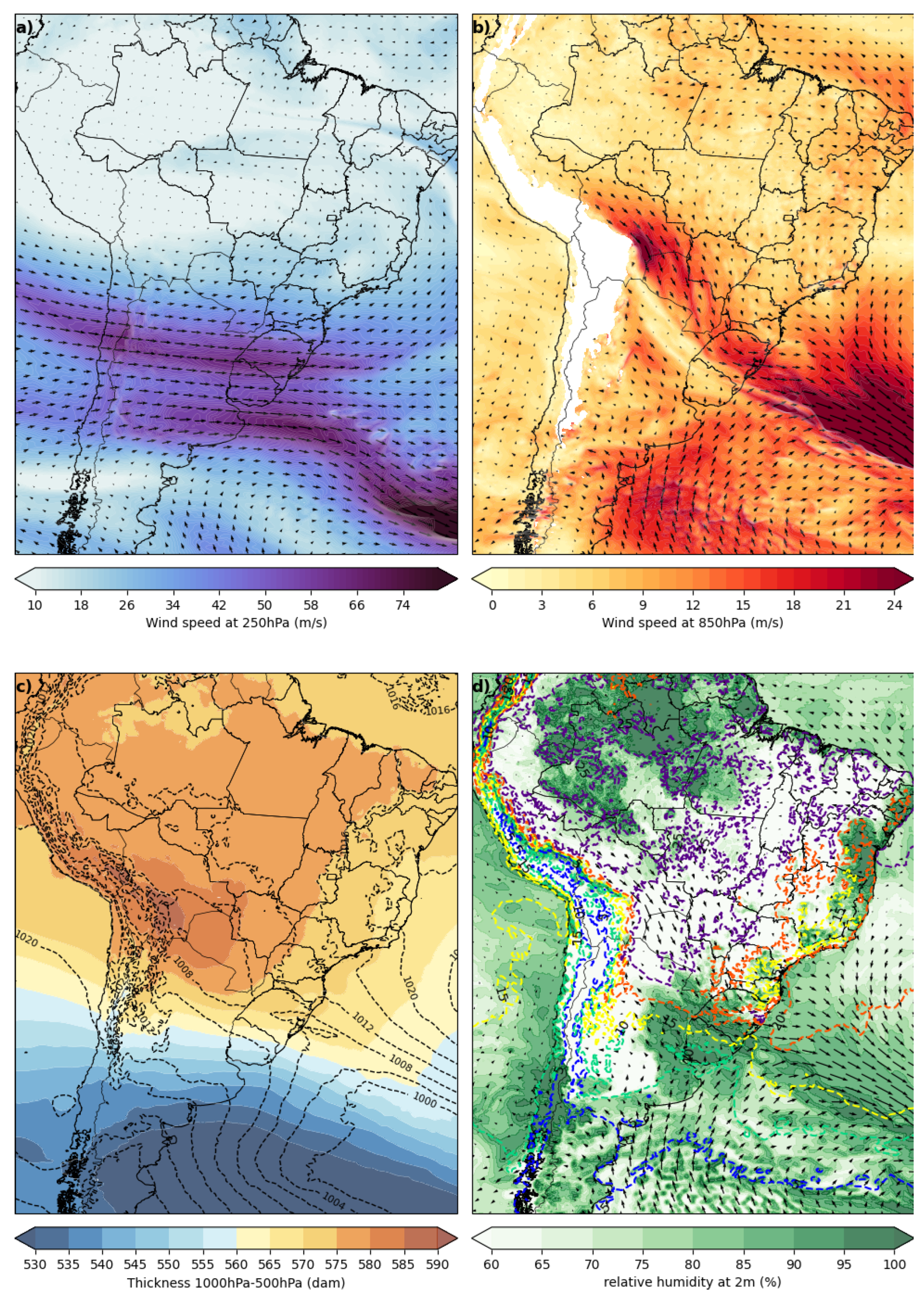
Two days before the event, at upper levels, Figure A3a shows an intensification of winds extending across southern Chile and Argentina, then curving eastward over the South Atlantic. The narrow wind speed gradient in the panel suggests the presence of a strong jet streak embedded within the broader westerly flow. In the region where upper-level wind acceleration occurs, a pronounced temperature contrast below can be observed (i.e., a strong north-south temperature gradient in the mid-levels), as seen in Figure A3c. This figure highlights how thickness contours compress in mid-latitudes, revealing a sharp north-south temperature contrast. Analyzing Figure A3b, an increase in the intensity of the LLJ can be identified, consistent with a robust low-level jet pulling warm, moist tropical air southward. This configuration is considered a classic setup for cyclogenesis development. Furthermore, in Figure A3c, this circulation provides the necessary supply of warm advection and moisture transport from the Amazon region toward the cyclogenesis development area. On the 17th, at upper levels, the jet’s displacement suggests that the upper-level ridge pattern has progressed eastward, a classic characteristic of a mid-latitude wave train. At lower levels, the northwest-southeast orientation of strong 850 hPa winds channels moist tropical air into mid-latitude systems. The area of maximum wind speed moved eastward, suggesting that the frontal boundary associated with the surface low is shifting toward the Atlantic. Examining Figure A3c, there is a possible deepening of a surface low, indicating the frontal system’s displacement over the southern region. Meanwhile, Figure A3d presents a near-surface temperature gradient over southern Brazil and northern Argentina, indicating its intensification as the front moves across the region. Throughout the 17th, in general, the jet shifted eastward, strengthening the low-level flow and frontal dynamics, while surface temperatures and moisture organized into a more sharply defined frontal zone, separating warm, moist tropical air from cooler air.
Figure A3.
Synoptic fields on August 17 at 0:00 UTC from the WRF model: a) Wind field up to 250 hPa; b)Wind field up to 850 hPa; c) Surface Pressure (isolines) and thickness 500-1000 hPa field (shaded contours); d) Wind field up to 850 hPa (vectors), temperature at 2m (isotherms) and relative humidity at 2m (shaded contours).
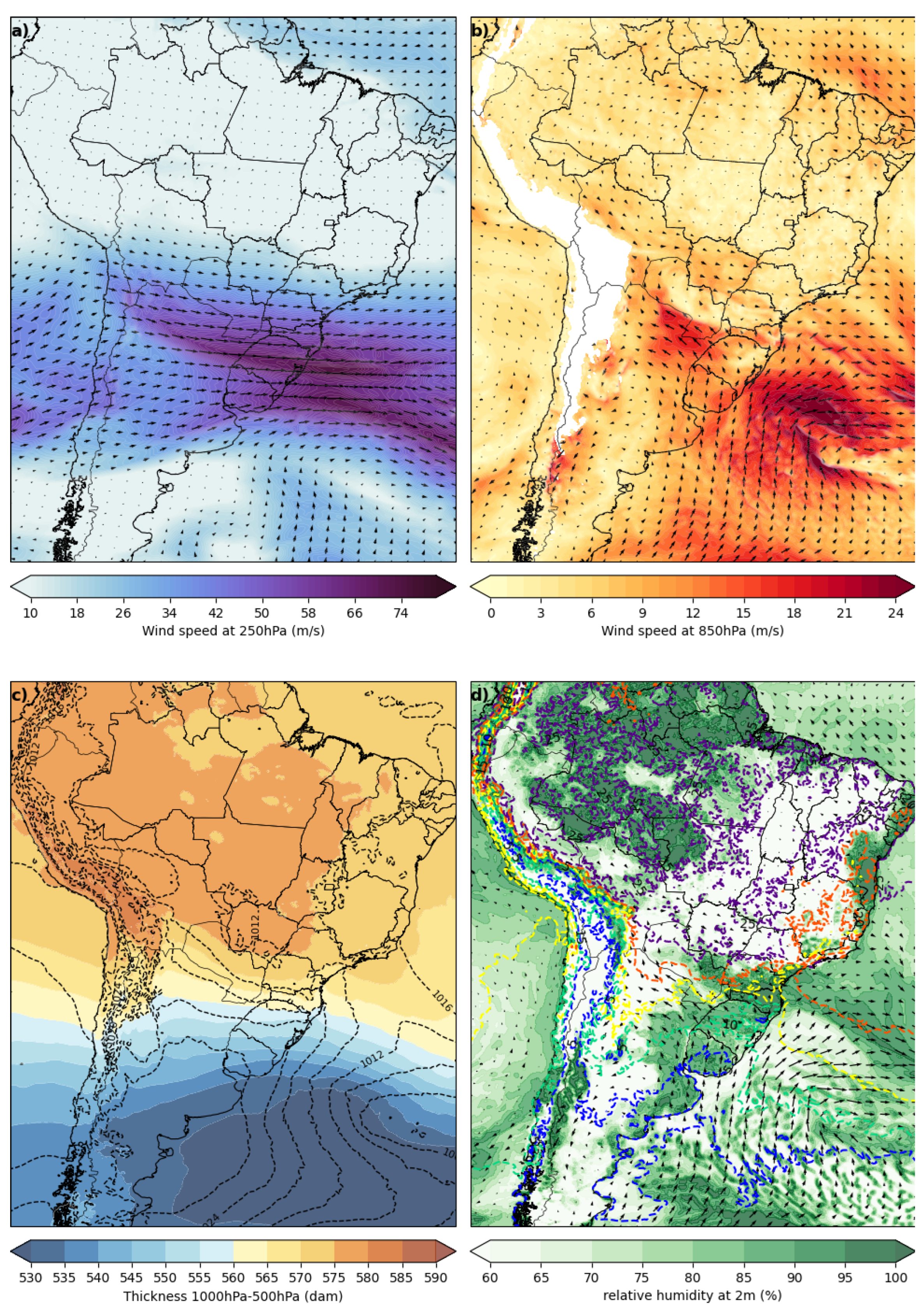
On August 18, the day begins with the advancement of the frontal system over the region of the state of Rio Grande do Sul, accompanied by moisture influx and warm advection from northern Brazil, as seen in Figure A4b,d. Meanwhile, in Figure A4c, the thickness gradient in the southern region corroborates the passage of the cold front. In the early hours of the day, this system moves over the states of Santa Catarina and Paraná, with the development of a cyclone over the Atlantic Ocean, near the coast, aiding in the convergence of low-level winds. This change in low-level wind direction helped shift the area affected by particulates originating from biomass burning. By the end of the day, the region of interest—namely, São Paulo—is impacted by the transport of these particulates. This frontal system will favor the development of cloud cover through lifting and, consequently, precipitation. In this case, aerosols can serve as condensation nuclei (CNNs). At upper levels, the jet has its core centered over the oceanic region, near the occluded system (which is already outside the domain) during the early hours of the day. However, as the cyclone develops over the open sea, the jet intensifies over Brazil. In the upper part of the jet, studies indicate the presence of an area of ascent, suggesting that the regions of Paraná and São Paulo have the necessary ingredients for convective development, supported by moisture influx and high temperatures due to the advancement of the frontal system, combined with the positioning of the upper-level jet.
Figure A4.
Synoptic fields on August 18 at 0:00 UTC from the WRF model: a) Wind field up to 250 hPa; b)Wind field up to 850 hPa; c) Surface Pressure (isolines) and thickness 500-1000 hPa field (shaded contours); d) Wind field up to 850 hPa (vectors), temperature at 2m (isotherms) and relative humidity at 2m (shaded contours).
When analyzing the synoptic fields on the day of the event, August 19th, it can be observed from Figure A5b–d that the cyclone primarily moved longitudinally during the early hours, with minimal latitudinal displacement. This is evident from the isobars in the pressure field, the wind circulation at the 850 hPa level, and the convergence of relative humidity. A notable point is the decrease in wind intensity in the regions where the highest concentration of particulates originates (central-western Brazil, parts of Bolivia, and Paraguay), indicating that the particulates used as CNN’s had already reached the region of interest, namely São Paulo, in the days prior. In the southern region, the advance of a high-pressure system behind the front favors stability over areas of Argentina and southern Brazil. At higher levels, similar to the previous day, the jet stream is positioned above the cyclone, indicating a baroclinic region. Studies such as that of [6] have focused on understanding the thermodynamics in the São Paulo region during the event day, indicating that when analyzing the vertical profile of temperature and dew point temperature, a significant thermal inversion was observed, hindering upward movements and causing the particulates to remain at lower levels. This highlights the direct impact of the frontal system on the dispersion of this material.
Figure A5.
Synoptic fields on August 19 at 0:00 UTC from the WRF model: a) Wind field up to 250 hPa; b)Wind field up to 850 hPa; c) Surface Pressure (isolines) and thickness 500-1000 hPa field (shaded contours); d) Wind field up to 850 hPa (vectors), temperature at 2m (isotherms) and relative humidity at 2m (shaded contours).
Appendix A.2. Daily Transport of Tracer’s
Figure A6.
Total column of passive tracers for August 15, 2019. The red color represents tr17_t1, the green color represents tr17_t2, and the blue color represents tr17_t3. Each column represents the PBL scheme used.
Figure A6.
Total column of passive tracers for August 15, 2019. The red color represents tr17_t1, the green color represents tr17_t2, and the blue color represents tr17_t3. Each column represents the PBL scheme used.
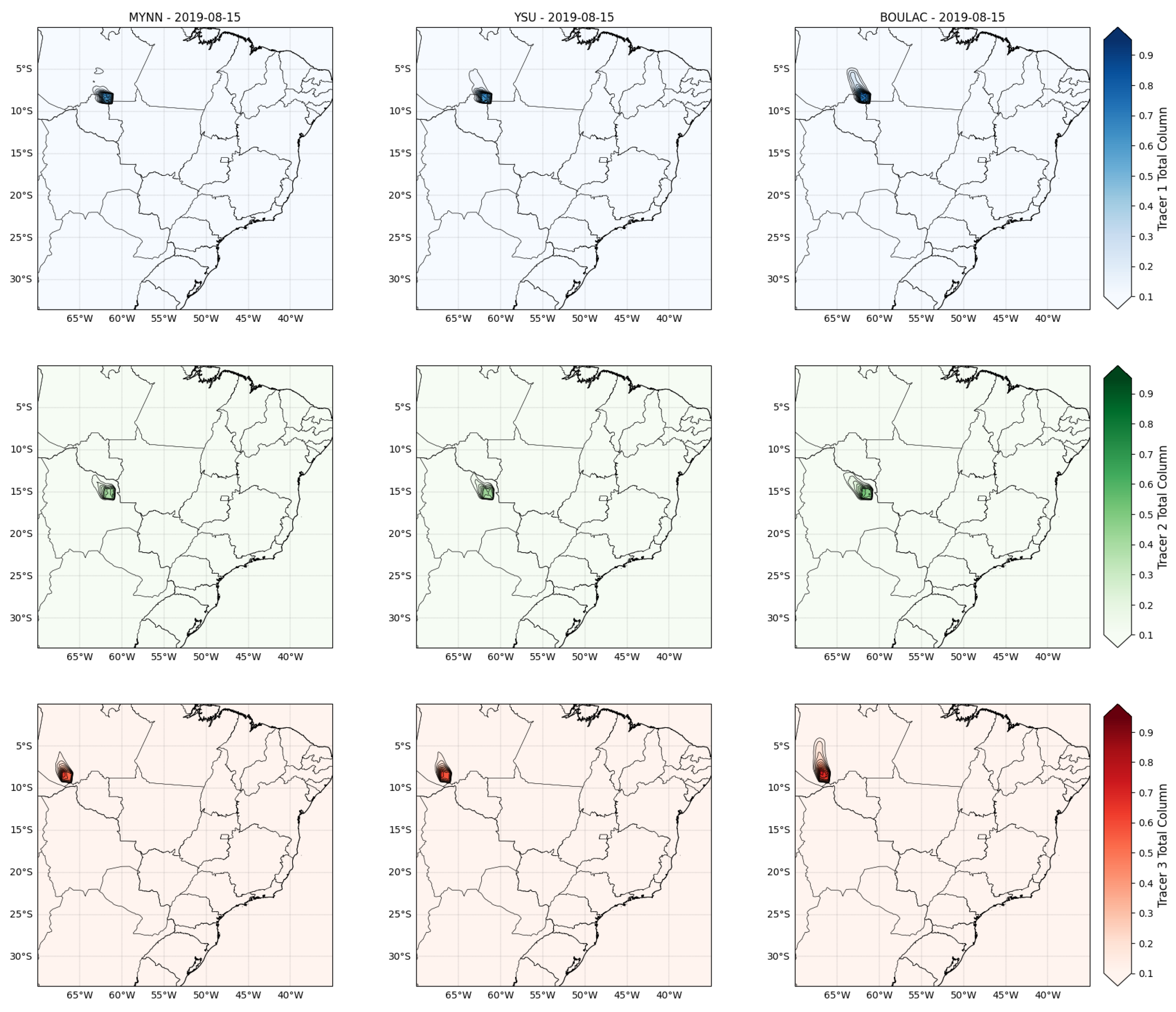
Figure A7.
Total column of passive tracers for August 16, 2019. The red color represents tr17_t1, the green color represents tr17_t2, and the blue color represents tr17_t3. Each column represents the PBL scheme used.
Figure A7.
Total column of passive tracers for August 16, 2019. The red color represents tr17_t1, the green color represents tr17_t2, and the blue color represents tr17_t3. Each column represents the PBL scheme used.
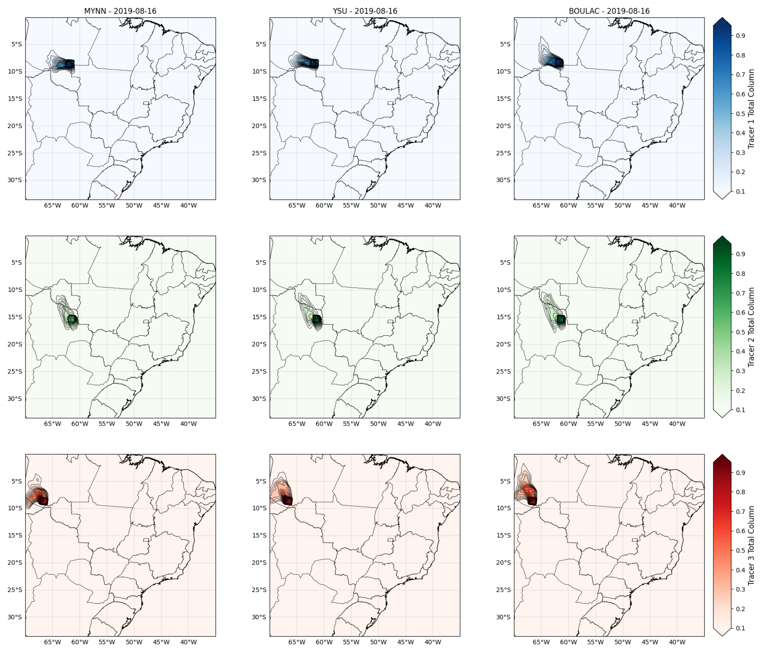
Figure A8.
Total column of passive tracers for August 17, 2019. The red color represents tr17_t1, the green color represents tr17_t2, and the blue color represents tr17_t3. Each column represents the PBL scheme used.
Figure A8.
Total column of passive tracers for August 17, 2019. The red color represents tr17_t1, the green color represents tr17_t2, and the blue color represents tr17_t3. Each column represents the PBL scheme used.
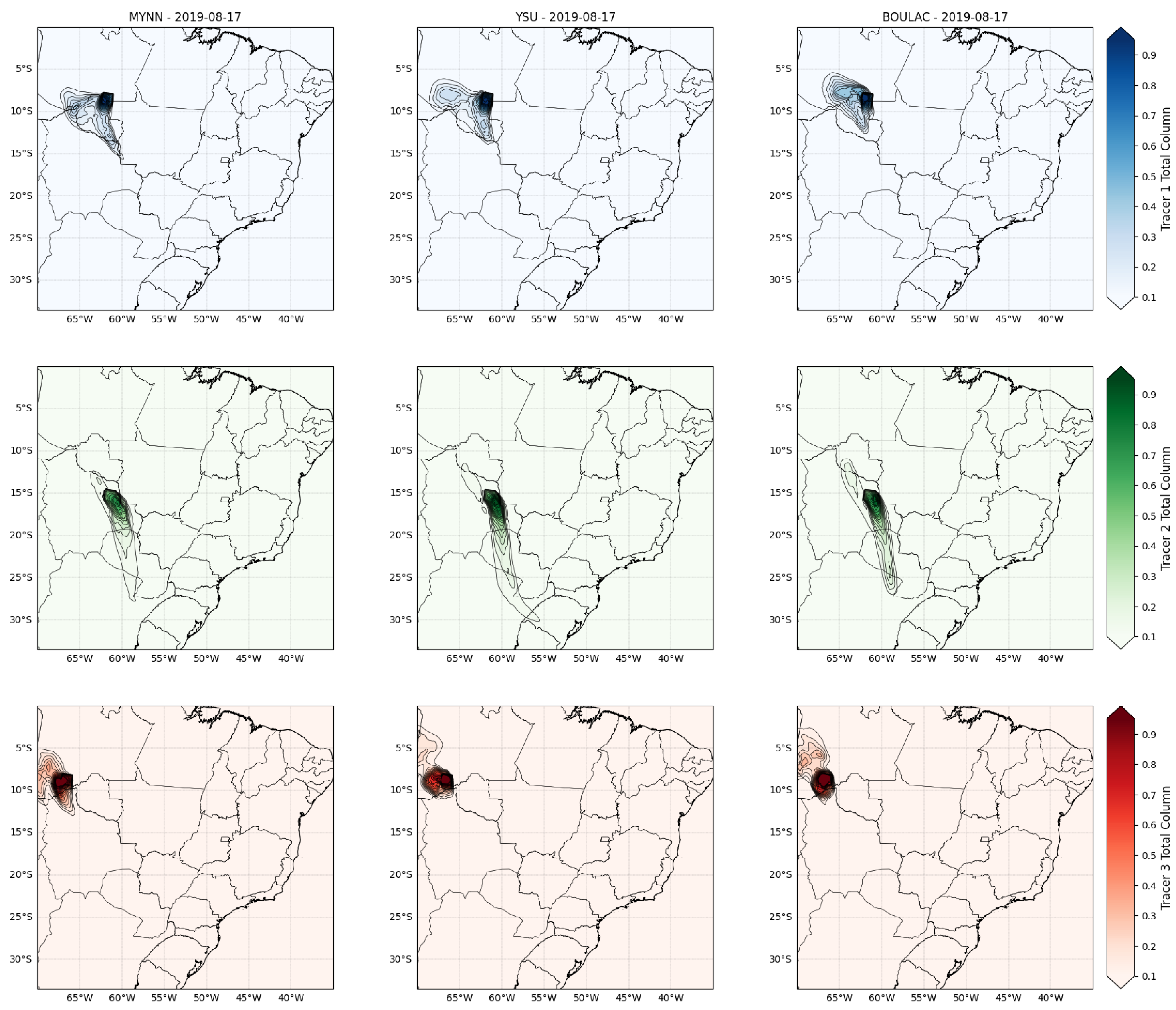
Figure A9.
Total column of passive tracers for August 18, 2019. The red color represents tr17_t1, the green color represents tr17_t2, and the blue color represents tr17_t3. Each column represents the PBL scheme used.
Figure A9.
Total column of passive tracers for August 18, 2019. The red color represents tr17_t1, the green color represents tr17_t2, and the blue color represents tr17_t3. Each column represents the PBL scheme used.
References
- Vitousek, P.M.; Mooney, H.A.; Lubchenco, J.; Melillo, J.M. Human domination of Earth’s ecosystems. Science 1997, 277, 494–499. [Google Scholar] [CrossRef]
- Forest, C.E.; Stone, P.H.; Sokolov, A.P.; Allen, M.R.; Webster, M.D. Quantifying uncertainties in climate system properties with the use of recent climate observations. science 2002, 295, 113–117. [Google Scholar] [CrossRef] [PubMed]
- RamanathanV, C.; et al. Atmosphere aerosols, climate, andthehydrologicalcycle. Science 2001, 294, 2119r2124. [Google Scholar] [CrossRef]
- Trickl, T.; Giehl, H.; Jäger, H.; Vogelmann, H. 35 yr of stratospheric aerosol measurements at Garmisch-Partenkirchen: from Fuego to Eyjafjallajökull, and beyond. Atmospheric Chemistry and Physics 2013, 13, 5205–5225. [Google Scholar] [CrossRef]
- Bencherif, H.; Bègue, N.; Kirsch Pinheiro, D.; Du Preez, D.J.; Cadet, J.M.; da Silva Lopes, F.J.; Shikwambana, L.; Landulfo, E.; Vescovini, T.; Labuschagne, C.; et al. Investigating the Long-Range Transport of Aerosol Plumes Following the Amazon Fires (August 2019): A Multi-Instrumental Approach from Ground-Based and Satellite Observations. Remote Sensing 2020, 12, 3846. [Google Scholar] [CrossRef]
- Lemes, M.; Reboita, M.S.; Capucin, B.C. Impactos das queimadas na Amazônia no tempo em São Paulo na tarde do dia 19 de agosto de 2019. Revista Brasileira de Geografia Física 2020, 13, 983–993. [Google Scholar] [CrossRef]
- Lima de Bem, D.; Anabor, V.; Dornelles Bittencourt, G.; Kirsch Pinheiro, D.; Scremin Puhales, F.; Bencherif, H.; Bègue, N.; Angelo Steffenel, L. Análise das condições sinóticas durante os incêndios florestais na Amazônia e seu impacto na cidade de São Paulo em 19 de agosto de 2019. Revista Ciência e Natura 2024, 46. [Google Scholar] [CrossRef]
- Copernicus. Observer: Monitoring fire emissions and mitigating global impacts with CAMS. https://www.copernicus.eu/en/news/news/observer-monitoring-fire-emissions-and-mitigating-global-impacts-cams. [Online; acessado em 28-fev-2025].
- Barbosa, H.A.; Buriti, C.O.; Kumar, T.V.L. Assessment of Fire Dynamics in the Amazon Basin Through Satellite Data. Atmosphere 2025, 16, 228. [Google Scholar] [CrossRef]
- Stull, R. An introduction to boundary layer meteorology; Kluwer Academic Publishers: Dordrecht, 1988; p. 666.
- Reid, J.; Koppmann, R.; Eck, T.; Eleuterio, D. A review of biomass burning emissions part II: intensive physical properties of biomass burning particles. Atmospheric chemistry and physics 2005, 5, 799–825. [Google Scholar] [CrossRef]
- Rogers, C.F.; Hudson, J.G.; Zielinska, B.; Tanner, R.L.; Hallett, J.; Watson, J.G. Cloud condensation nuclei from biomass burning 1991.
- Malavelle, F.F.; Haywood, J.M.; Mercado, L.M.; Folberth, G.A.; Bellouin, N.; Sitch, S.; Artaxo, P. Studying the impact of biomass burning aerosol radiative and climate effects on the Amazon rainforest productivity with an Earth system model. Atmospheric Chemistry and Physics 2019, 19, 1301–1326. [Google Scholar] [CrossRef]
- Li, Z.; Niu, F.; Fan, J.; Liu, Y.; Rosenfeld, D.; Ding, Y. Long-term impacts of aerosols on the vertical development of clouds and precipitation. Nature Geoscience 2011, 4, 888–894. [Google Scholar] [CrossRef]
- Tao, W.K.; Chen, J.P.; Li, Z.; Wang, C.; Zhang, C. Impact of aerosols on convective clouds and precipitation. Reviews of Geophysics 2012, 50. [Google Scholar] [CrossRef]
- Menzel, W.P.; Purdom, J.F. Introducing GOES-I: The first of a new generation of geostationary operational environmental satellites. Bulletin of the American Meteorological Society 1994, 75, 757–782. [Google Scholar] [CrossRef]
- Schmit, T.J.; Gunshor, M.M.; Menzel, W.P.; Gurka, J.J.; Li, J.; Bachmeier, A.S. Introducing the next-generation Advanced Baseline Imager on GOES-R. Bulletin of the American Meteorological Society 2005, 86, 1079–1096. [Google Scholar] [CrossRef]
- Schmidt, C. Monitoring fires with the GOES-R series. In The GOES-R Series; Elsevier, 2020; pp. 145–163.
- Roberts, G.J.; Wooster, M.J. Fire detection and fire characterization over Africa using Meteosat SEVIRI. IEEE Transactions on Geoscience and Remote Sensing 2008, 46, 1200–1218. [Google Scholar] [CrossRef]
- Hall, J.; Schroeder, W.; Rishmawi, K.; Wooster, M.; Schmidt, C.; Huang, C.; Csiszar, I.; Giglio, L. Geostationary active fire products validation: GOES-17 ABI, GOES-16 ABI, and Himawari AHI. International Journal of Remote Sensing 2023, 44, 3174–3193. [Google Scholar] [CrossRef]
- Hall, J.V.; Zhang, R.; Schroeder, W.; Huang, C.; Giglio, L. Validation of GOES-16 ABI and MSG SEVIRI active fire products. International Journal of Applied Earth Observation and Geoinformation 2019, 83, 101928. [Google Scholar] [CrossRef]
- Wu, X.; Schmit, T. GOES-16 ABI level 1b and cloud and moisture imagery (CMI) release full validation data quality. Nat. Centers Environ. Inf.(NCEI), College Park, MD, USA, Tech. Rep 2019, 1. [Google Scholar]
- Schmidt, C.; Hoffman, J.; Prins, E.; Lindstrom, S. GOES-R advanced baseline imager (ABI) algorithm theoretical basis document for fire/hot spot characterization, version 2.0, NOAA, Silver Spring, Md, 2010.
- William C Skamarock, Joseph B, J.D.; et al. Weather Forecast and Research Model, 2021. [CrossRef]
- C3S. ERA5, 2017.
- Iacono, M.J.; Delamere, J.S.; Mlawer, E.J.; Shephard, M.W.; Clough, S.A.; Collins, W.D. Radiative forcing by long-lived greenhouse gases. Journal of Geophysical Research: Atmospheres 2008, 113, 1–8. [Google Scholar] [CrossRef]
- Jiménez, P.A.; Dudhia, J.; González-Rouco, J.F.; Navarro, J.; Montávez, J.P.; García-Bustamante, E. A Revised Scheme for the WRF Surface Layer Formulation. Monthly weather review 2012, 140, 898–918. [Google Scholar] [CrossRef]
- Grell, G.A.; Freitas, S.R. A scale and aerosol aware stochastic convective parameterization for weather and air quality modeling. Atmospheric Chemistry and Physics 2014, 14, 5233–5250. [Google Scholar] [CrossRef]
- Hong, S.Y.; Lim, J.O.J. The WRF single-moment 6-class microphysics scheme (WSM6). Asia-Pacific Journal of Atmospheric Sciences 2006, 42, 129–151. [Google Scholar]
- Nakanishi, M.; Niino, H. Development of an improved turbulence closure model for the atmospheric boundary layer. Journal of the Meteorological Society of Japan. Ser. II 2009, 87, 895–912. [Google Scholar] [CrossRef]
- Janjić, Z.I. The step-mountain eta coordinate model: Further developments of the convection, viscous sublayer, and turbulence closure schemes. Monthly weather review 1994, 122, 927–945. [Google Scholar] [CrossRef]
- Mesinger, F. Forecasting upper tropospheric turbulence within the framework of the Mellor-Yamada 2.5 closure. Research activities in atmospheric and oceanic modeling. Technical report, WMO/CAS/JSC WGNE Tech. Rep. 18, 1993.
- Bougeault, P.; Lacarrere, P. Parameterization of orography-induced turbulence in a mesobeta–scale model. Monthly weather review 1989, 117, 1872–1890. [Google Scholar] [CrossRef]
- Hong, S.Y.; Lim, J.O.J. The WRF single-moment 6-class microphysics scheme (WSM6). Asia-Pacific Journal of Atmospheric Sciences 2006, 42, 129–151. [Google Scholar]
- Hong, S.Y.; Pan, H.L. Nonlocal boundary layer vertical diffusion in a medium-range forecast model. Monthly weather review 1996, 124, 2322. [Google Scholar] [CrossRef]
- Saffman, P. On the effect of the molecular diffusivity in turbulent diffusion. Journal of Fluid Mechanics 1960, 8, 273–283. [Google Scholar] [CrossRef]
- Njuki, S.M.; Mannaerts, C.M.; Su, Z. Influence of Planetary Boundary Layer (PBL) Parameterizations in the Weather Research and Forecasting (WRF) model on the retrieval of surface meteorological variables over the Kenyan Highlands. Atmosphere 2022, 13, 169. [Google Scholar] [CrossRef]
- Gunwani, P.; Govardhan, G.; Jena, C.; Yadav, P.; Kulkarni, S.; Debnath, S.; Pawar, P.V.; Khare, M.; Kaginalkar, A.; Kumar, R.; et al. Sensitivity of WRF/Chem simulated PM2. 5 to initial/boundary conditions and planetary boundary layer parameterization schemes over the Indo-Gangetic Plain. Environmental Monitoring and Assessment 2023, 195, 560. [Google Scholar] [CrossRef]
- Blaylock, B.K.; Horel, J.D.; Crosman, E.T. Impact of lake breezes on summer ozone concentrations in the Salt Lake valley. Journal of Applied Meteorology and Climatology 2017, 56, 353–370. [Google Scholar] [CrossRef]
- Bhimireddy, S.R.; Bhaganagar, K. Short-term passive tracer plume dispersion in convective boundary layer using a high-resolution WRF-ARW model. Atmospheric Pollution Research 2018, 9, 901–911. [Google Scholar] [CrossRef]
- Fathi, S.; Gordon, M.; Chen, Y. Passive-tracer modelling at super-resolution with Weather Research and Forecasting–Advanced Research WRF (WRF-ARW) to assess mass-balance schemes. Geoscientific Model Development 2023, 16, 5069–5091. [Google Scholar] [CrossRef]
- Yang, Q.; Easter, R.C.; Campuzano-Jost, P.; Jimenez, J.L.; Fast, J.D.; Ghan, S.J.; Wang, H.; Berg, L.K.; Barth, M.C.; Liu, Y.; et al. Aerosol transport and wet scavenging in deep convective clouds: A case study and model evaluation using a multiple passive tracer analysis approach. Journal of Geophysical Research: Atmospheres 2015, 120, 8448–8468. [Google Scholar] [CrossRef]
- Bhimireddy, S.R.; Bhaganagar, K. Performance assessment of dynamic downscaling of WRF to simulate convective conditions during sagebrush phase 1 tracer experiments. Atmosphere 2018, 9, 505. [Google Scholar] [CrossRef]
- Saide, P.E.; Carmichael, G.R.; Spak, S.N.; Gallardo, L.; Osses, A.E.; Mena-Carrasco, M.A.; Pagowski, M. Forecasting urban PM10 and PM2. 5 pollution episodes in very stable nocturnal conditions and complex terrain using WRF–Chem CO tracer model. Atmospheric Environment 2011, 45, 2769–2780. [Google Scholar] [CrossRef]
- Davies, D.; Ederer, G.; Olsina, O.; Wong, M.; Cechini, M.; Boller, R. NASA’s fire information for resource management system (FIRMS): Near real-time global fire monitoring using data from MODIS and VIIRS. In Proceedings of the EARSel Forest Fires SIG Workshop, 2019, number GSFC-E-DAA-TN73770.
- Olsina, O.; Hewson, J.; Davies, D.; Radov, A.; Quayle, B.; Giglio, L.; Hall, J. NASA’s FIRMS: Enabling the Use of Earth System Science Data for Wildfire Management. Technical report, Copernicus Meetings, 2024. [CrossRef]
- Chauvigné, A.; Aliaga, D.; Sellegri, K.; Montoux, N.; Krejci, R.; Močnik, G.; Moreno, I.; Müller, T.; Pandolfi, M.; Velarde, F.; et al. Biomass burning and urban emission impacts in the Andes Cordillera region based on in situ measurements from the Chacaltaya observatory, Bolivia (5240 m asl). Atmospheric chemistry and physics 2019, 19, 14805–14824. [Google Scholar] [CrossRef]
- Yin, S.; Wang, X.; Zhang, X.; Guo, M.; Miura, M.; Xiao, Y. Influence of biomass burning on local air pollution in mainland Southeast Asia from 2001 to 2016. Environmental Pollution 2019, 254, 112949. [Google Scholar] [CrossRef]
- Schafer, J.; Eck, T.; Holben, B.; Artaxo, P.; Yamasoe, M.A.; Procopio, A. Observed reductions of total solar irradiance by biomass-burning aerosols in the Brazilian Amazon and Zambian Savanna. Geophysical Research Letters 2002, 29, 4–1. [Google Scholar] [CrossRef]
- Landulfo, E.; Papayannis, A.; Artaxo, P.; Castanho, A.; De Freitas, A.; Souza, R.; Vieira, N.; Jorge, M.; Sánchez-Ccoyllo, O.; Moreira, D. Synergetic measurements of aerosols over São Paulo, Brazil using LIDAR, sunphotometer and satellite data during the dry season. Atmospheric Chemistry and Physics 2003, 3, 1523–1539. [Google Scholar] [CrossRef]
- Lopes, F.; Silva, J.; Antuña Marrero, J.; Taha, G.; Landulfo, E. Synergetic Aerosol Layer Observation After the 2015 Calbuco Volcanic Eruption Event, Remote Sens., 11, 195, 2019. [CrossRef]
- Stensrud, D.J. Importance of low-level jets to climate: A review. Journal of Climate 1996, pp. 1698–1711. https://doi.org/https://www.jstor.org/stable/26201369.
- Vera, C.; Baez, J.; Douglas, M.; Emmanuel, C.; Marengo, J.; Meitin, J.; Nicolini, M.; Nogues-Paegle, J.; Paegle, J.; Penalba, O.; et al. The South American low-level jet experiment. Bulletin of the American Meteorological Society 2006, 87, 63–78. [Google Scholar] [CrossRef]
- Abish, B.; Joseph, P.; Johannessen, O.M. Climate change in the subtropical jetstream during 1950–2009. Advances in Atmospheric Sciences 2015, 32, 140–148. [Google Scholar] [CrossRef]
Figure 1.
GOES-16 true-color of the South America during days 15 (a), 16 (b), 17 (c), 18 (d), and 19 (e) of August 2019 at 18:00 UTC, with fire-detected pixels overlaid in red.
Figure 1.
GOES-16 true-color of the South America during days 15 (a), 16 (b), 17 (c), 18 (d), and 19 (e) of August 2019 at 18:00 UTC, with fire-detected pixels overlaid in red.
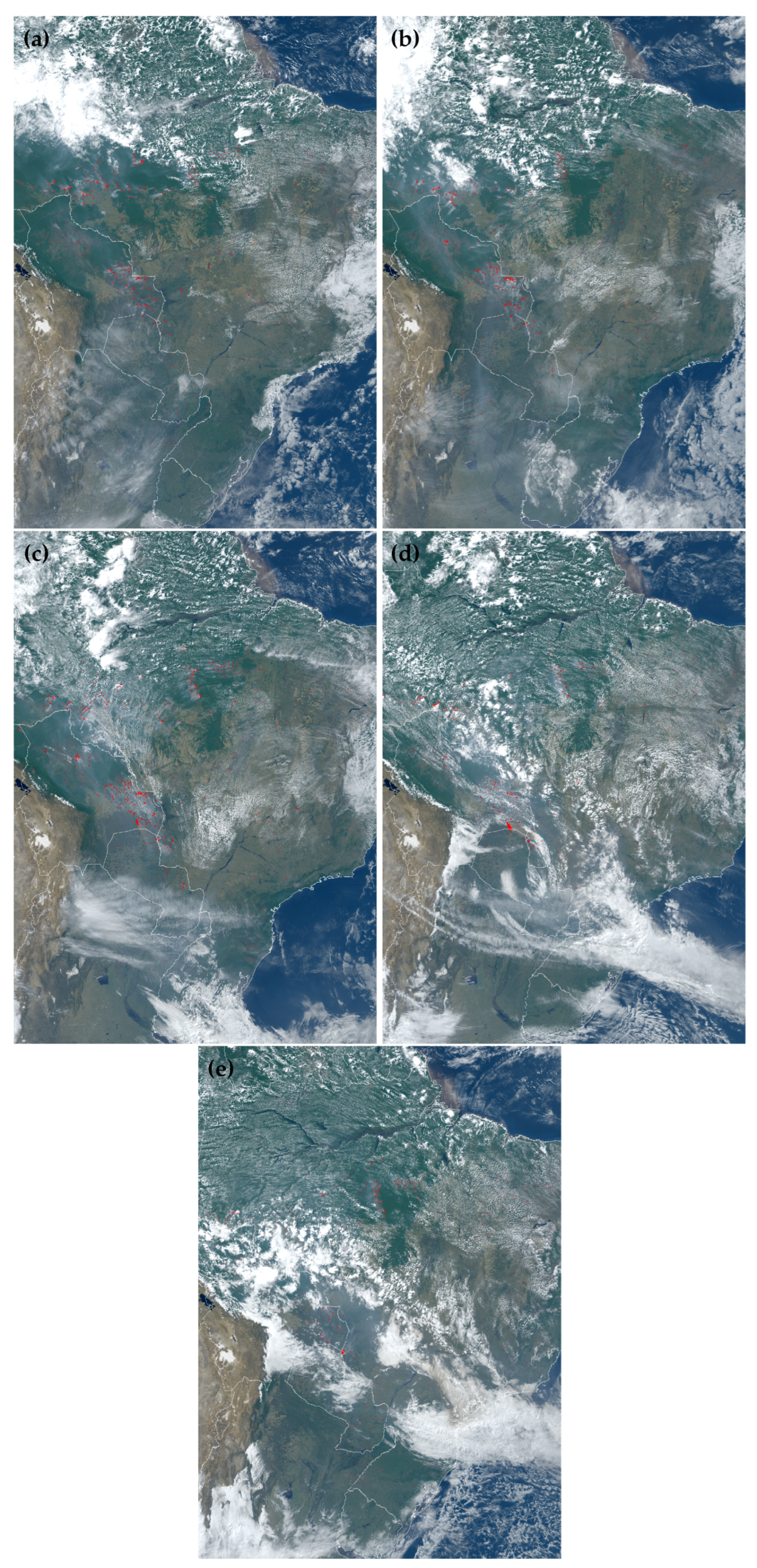
Figure 3.
FIRMS Fire Radiate Power Pixel to study area. The black circle represents the area with the highest concentration of fire pixels.
Figure 3.
FIRMS Fire Radiate Power Pixel to study area. The black circle represents the area with the highest concentration of fire pixels.
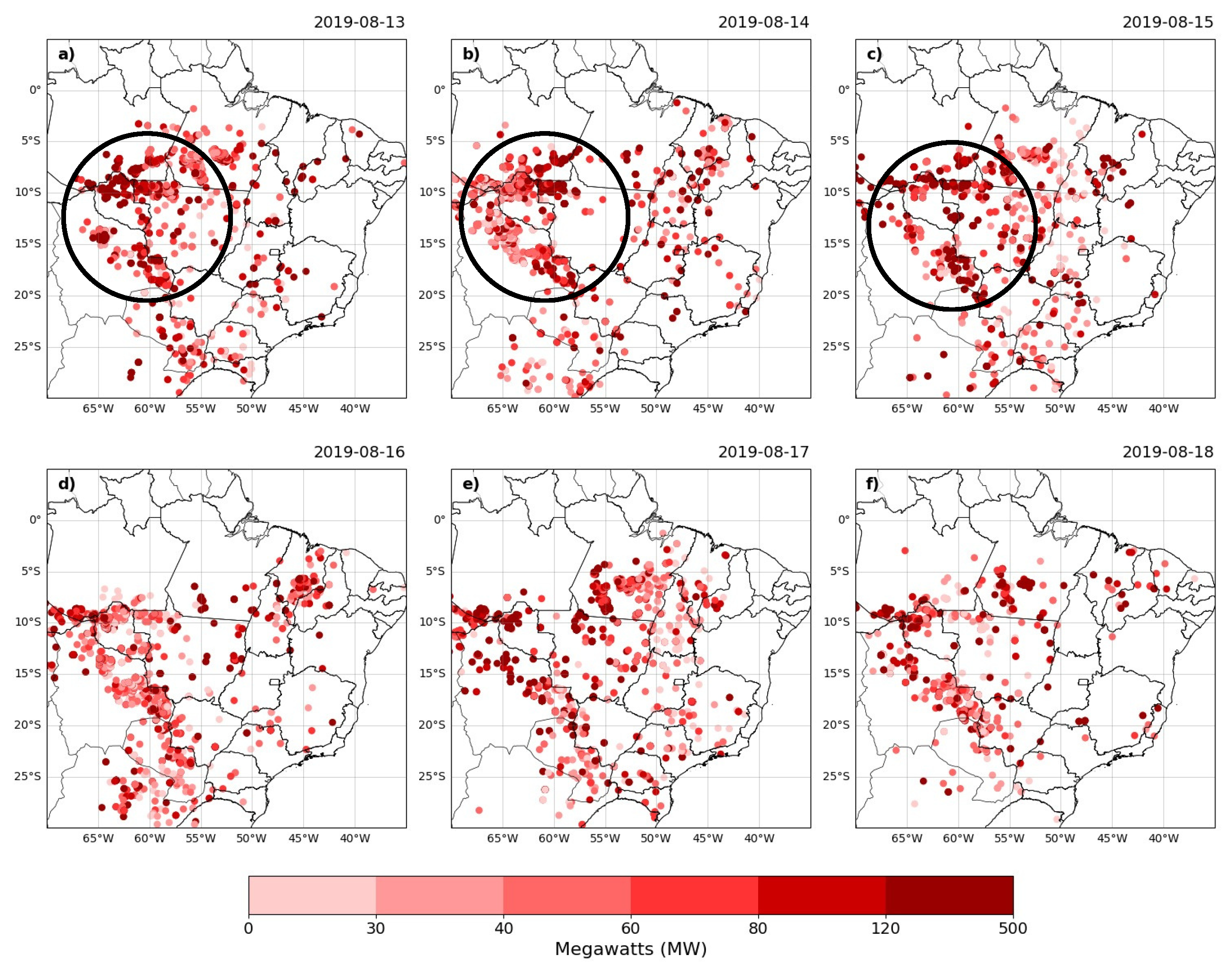
Figure 4.
Total column of passive tracers for August 19, 2019. The red color represents tr17_t1, the green color represents tr17_t2, and the blue color represents tr17_t3. Each column represents the PBL scheme used.
Figure 4.
Total column of passive tracers for August 19, 2019. The red color represents tr17_t1, the green color represents tr17_t2, and the blue color represents tr17_t3. Each column represents the PBL scheme used.
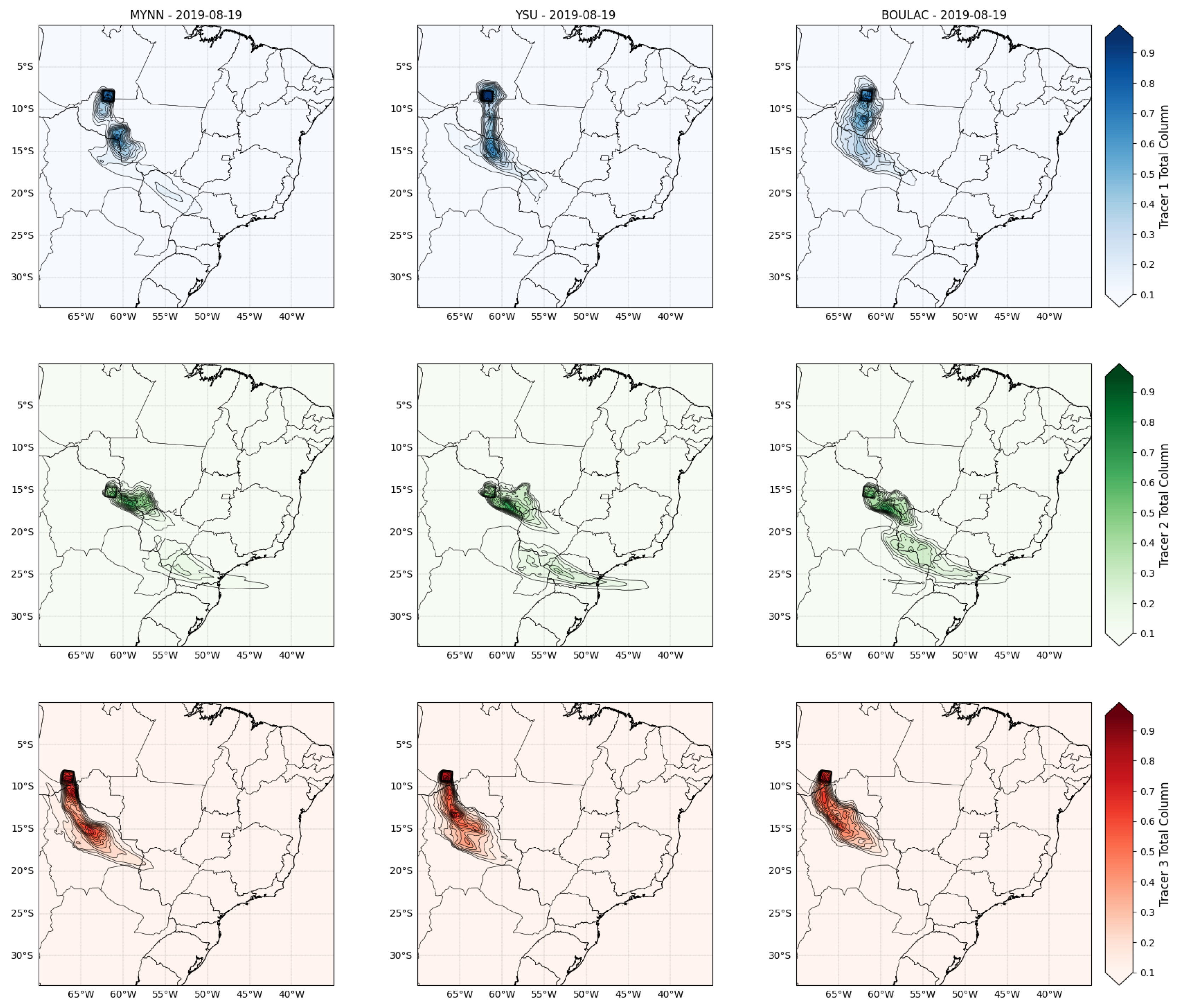
Figure 6.
Time-height cross-sections of tr17_t1 in São Paulo during the simulation period for the three schemes (MYNN, YSU, and BouLac).
Figure 6.
Time-height cross-sections of tr17_t1 in São Paulo during the simulation period for the three schemes (MYNN, YSU, and BouLac).
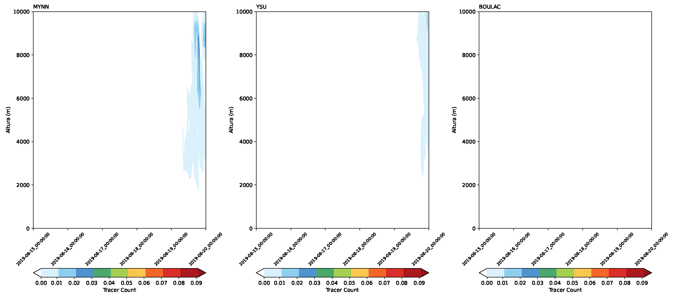
Figure 7.
Time-height cross-sections of tr17_t2 in São Paulo during the simulation period for the three schemes (MYNN, YSU, and BouLac).
Figure 7.
Time-height cross-sections of tr17_t2 in São Paulo during the simulation period for the three schemes (MYNN, YSU, and BouLac).
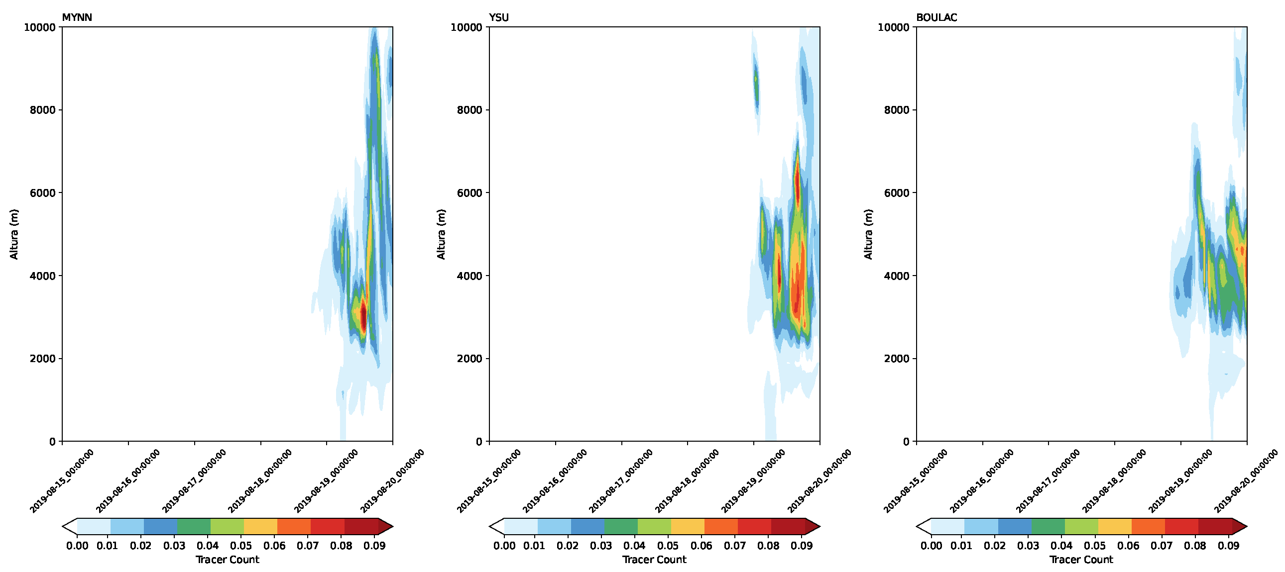
Figure 8.
Time-height cross-sections of tr17_t3 in São Paulo during the simulation period for the three schemes (MYNN, YSU, and BouLac).
Figure 8.
Time-height cross-sections of tr17_t3 in São Paulo during the simulation period for the three schemes (MYNN, YSU, and BouLac).
Disclaimer/Publisher’s Note: The statements, opinions and data contained in all publications are solely those of the individual author(s) and contributor(s) and not of MDPI and/or the editor(s). MDPI and/or the editor(s) disclaim responsibility for any injury to people or property resulting from any ideas, methods, instructions or products referred to in the content. |
© 2025 by the authors. Licensee MDPI, Basel, Switzerland. This article is an open access article distributed under the terms and conditions of the Creative Commons Attribution (CC BY) license (http://creativecommons.org/licenses/by/4.0/).
Copyright: This open access article is published under a Creative Commons CC BY 4.0 license, which permit the free download, distribution, and reuse, provided that the author and preprint are cited in any reuse.


