
Submitted:
10 January 2026
Posted:
12 January 2026
You are already at the latest version
Abstract
In the seismic design of reinforced concrete moment-resisting frame (RC MRF) structures equipped with steel damper columns (SDCs), design criteria should consider both peak responses (e.g., story drift) and cumulative responses (e.g., cumulative strain energy of damper panels in SDCs). These response measures are associated with two energy-based seismic intensity parameters: the maximum momentary input energy governing peak responses and the cumulative input energy governing cumulative responses. The relationship between these parameters depends on the characteristics of the ground motions. This study proposes an energy-based limit curve for RC MRFs with SDCs using the two seismic intensity parameters. Incremental critical pseudo-multi impulse analyses (ICPMIAs) are performed for three eight-story RC MRFs with SDCs considering various numbers of pulsive inputs. For each analysis, the input intensity is incrementally increased until predefined limit-state criteria are reached. The limit curve is constructed by connecting the equivalent velocity pairs corresponding to the two energy-based seismic intensity parameters at the limit states. The applicability of the proposed limit curve is examined through nonlinear time-history analyses (NTHAs) using recorded ground motions, including the mainshock–aftershock sequence of the 2011 off the Pacific coast of Tohoku Earthquake and the foreshock–mainshock sequence of the 2016 Kumamoto Earthquake. The results indicate that (a) considering a range of 2 to 32 pulsive inputs in ICPMIA is sufficient to cover the NTHA results examined in this study; (b) most NTHA cases satisfying the limit-state criteria are located within the proposed limit curve, whereas cases exceeding the criteria are located outside the curve; and (c) the consideration of earthquake sequences tends to result in a larger number of cases exceeding the limit-state criteria compared with single-earthquake scenarios.
Keywords:
reinforced concrete moment-resisting frame (RC MRF)
; steel damper column (SDC)
; incremental critical pseudo-multi impulse analysis (ICPMIA)
; maximum momentary input energy
; cumulative input energy
1. Introduction
1.1. Background and Motivations
In Japan, the use of seismic dampers in mid- and high-rise reinforced concrete (RC) residential buildings has been increasing in order to achieve enhanced seismic performance. Such RC moment-resisting frames (MRFs) equipped with seismic dampers can be regarded as damage-tolerant structures (Wada et al., 2000). During large seismic events, these dampers are designed to absorb a significant portion of the seismic energy input, thereby minimizing damage to beams and columns. Steel damper columns (SDCs; Katayama et al., 2000) are one type of seismic damper. In the authors’ research group, the seismic design of RC MRFs with SDCs has been investigated in previous studies (e.g., Mukouyama et al., 2021). Figure 1a illustrates an RC MRF with SDCs. The damper panel installed at the mid-height of an SDC is intended to yield prior to the formation of potential plastic hinge zones at the ends of RC beams and columns, thereby initiating the dissipation of seismic energy.
It is widely recognized that the concept of seismic energy input is essential for discussing the nonlinear seismic response of building structures, including damage-tolerant systems such as those described above. Recent achievements and progress in Energy-Based Seismic Engineering (EBSE) have been reported in the literature (Benavent-Climent and Mollaioli, 2021; Varum et al., 2023; Dindar et al., 2025). Akiyama (1985, 1999) introduced a seismic design framework based on cumulative energy input. The cumulative input energy (EI) proposed by Akiyama (1985) is one of the key input energy parameters associated with cumulative structural responses. Meanwhile, Inoue and his research group (Hori et al., 2000; Inoue et al., 2000; Hori and Inoue, 2002) introduced another essential input energy parameter, the maximum momentary input energy (), which has been shown to be suitable for evaluating the peak responses of RC MRFs. Figure 1b illustrates the relationships between essential response parameters of an RC MRF with SDCs and the corresponding input energy parameters. As shown on the left side of Figure 1b, the essential response parameters of an RC MRF with SDCs can be classified into two groups: peak responses and cumulative responses. The peak response group includes (i) story drift of the MRF, (ii) plastic hinge rotation of RC beams and columns, and (iii) shear deformation of the damper panel. The cumulative response group includes the cumulative strain energy of the damper panel. In this figure, the cumulative strain energy of RC beams and columns is not explicitly considered. This modeling choice reflects the design concept of RC MRFs with SDCs, in which seismic energy dissipation is primarily intended to occur in the damper panels, while damage to RC members is controlled. The criteria and assumptions underlying this treatment are described in detail in Section 2.2. As summarized in Figure 1b, the maximum momentary input energy () is primarily related to peak responses, whereas the cumulative input energy () is associated with cumulative responses. Therefore, both and should be appropriately considered in the seismic design of RC MRFs with SDCs.
The relationship between and strongly depends on the characteristics of ground motions. Differences in structural responses associated with different ground motion records are illustrated on the left side of Figure 1c. For near-fault records characterized by forward-directivity or fling-step effects, the structural response is dominated by large peak deformations occurring within a small number of loading cycles. In contrast, long-duration records tend to induce a large number of cyclic loadings, as discussed by Kalkan and Kunnath (2006). Consequently, the ratio of the two input energy parameters () tends to be large for near-fault records and small for long-duration records. This implies that whether peak responses or cumulative responses become critical for an RC MRF with SDCs depends on the ratio . Therefore, when performance criteria for RC MRFs with SDCs are defined in terms of the response parameters shown on the left side of Figure 1b, it is reasonable to express the limit intensity of ground motions using both and .As illustrated on the right side of Figure 1c, an – plane can be considered for this purpose. For a given ground motion record, a point on this plane can be determined from nonlinear time-history analysis (NTHA) of an RC MRF with SDCs by scaling the record until one of the response parameters reaches its prescribed limit. By repeating this procedure for different ground motion records and connecting the resulting points, a limit curve representing the seismic capacity of the RC MRF with SDCs can be defined. However, due to the wide variability in the frequency characteristics of ground motion records, it is generally difficult to obtain a unique limit curve directly from recorded ground motions alone.
1.2. Brief Review of Related Studies
The evaluation of structural damage considering both peak and cumulative responses has been extensively studied by many researchers (e.g., Banon and Veneziano, 1982; Park and Ang, 1985; Park et al., 1985; Cosenza et al., 1993; Chai et al., 1995; Teran-Gilmore and Jirsa, 2005; Poljanšek and Fajfar, 2008; Rodrigues et al., 2013; Tropea et al., 2023, 2025a, 2025b). Among the early studies, Banon and Veneziano (1982) first proposed the use of two damage indicators—the inverse of the secant stiffness degradation ratio and the normalized cumulative strain energy—for evaluating damage in RC members. Park and Ang (1985) subsequently proposed a damage index expressed as a linear combination of peak deformation and cumulative strain energy, which was calibrated using nonlinear time-history analyses of damaged buildings reported in a companion study (Park et al., 1985). Cosenza et al. (1993) compared the nonlinear strength demand of single-degree-of-freedom (SDOF) systems subjected to given ground motions using different damage models, including those proposed by Banon and Veneziano (1982), Park and Ang (1985), and a linear cumulative plastic fatigue model. They showed that comparable nonlinear strength demands could be obtained by appropriately calibrating the parameters of these damage models. Chai et al. (1995) modified the Park–Ang damage model to account explicitly for plastic strain energy dissipated under monotonic loading conditions. Teran-Gilmore and Jirsa (2005) proposed an energy-based model to predict low-cycle fatigue damage. Poljanšek and Fajfar (2008) developed a damage model for RC MRFs that evaluates deformation capacity as a function of monotonic deformation capacity and hysteretic energy dissipation. Rodrigues et al. (2013) further extended the Park–Ang model for RC columns subjected to bidirectional loading based on experimental results. More recently, Tropea et al. (2023, 2025a) proposed an energy-based damage metric incorporating both hysteretic dissipated energy and its time derivative (“power”) and applied it to the seismic capacity evaluation of RC columns (Tropea et al., 2025b).
An important advantage of energy-based damage indices (e.g., Park and Ang, 1985; Poljanšek and Fajfar, 2008) is that they are closely linked to energy-based seismic intensity measures, which explicitly reflect ground motion characteristics. Ordaz et al. (2003) showed that the cumulative input energy () per unit mass can be directly calculated from the Fourier amplitude of ground motions. Similarly, the authors’ research group demonstrated that the maximum momentary input energy () per unit mass can be derived from the complex Fourier amplitude (Fujii et al., 2021).
The relationship between energy-based parameters and peak displacement has also been widely investigated in previous studies (e.g., Fajfar, 1992; Akiyama, 1999; Decanini et al., 2000; Manfredi et al., 2003; Kalkan and Kunnath, 2007; Benavent-Climent, 2011; Mota-Páez et al., 2021; Angelucci et al., 2023a, 2023b). Early studies proposed nondimensional parameters linking cumulative energy demand to peak deformation, such as Fajfar’s parameter (Fajfar, 1992) and the parameter introduced by Decanini et al. (2000). Akiyama (1999) further introduced the concept of an equivalent number of cycles, defined as the ratio of cumulative hysteretic energy to the hysteretic energy dissipated per cycle. Subsequent studies highlighted the influence of ground-motion characteristics on the relative importance of peak and cumulative demands. For example, Kalkan and Kunnath (2007) showed that structural response under near-fault ground motions is dominated by peak demand, whereas cumulative damage becomes more significant for far-field motions. Similar observations were reported in later studies focusing on near-fault and far-field effects (e.g., Mota-Páez et al., 2021).
In parallel with these empirical approaches, Inoue and his research group (Hori et al., 2000; Inoue et al., 2000; Hori and Inoue, 2002) proposed a more direct energy-based method to predict peak displacement using the maximum momentary input energy (), derived from the energy balance over a half cycle of structural response. Building on this framework, recent studies have further explored the relationship between peak and cumulative responses through the ratio , and have proposed simplified procedures for estimating both peak deformation and cumulative energy demand in RC MRFs with SDCs (e.g., Fujii and Shioda, 2023).
Akehashi and Takewaki (2021, 2022) proposed the critical pseudo-double impulse (PDI) analysis and the critical pseudo-multi impulse (PMI) analysis to evaluate the single-mode response of multi-degree-of-freedom (MDOF) systems subjected to critical ground-motion inputs. In these approaches, the critical double impulse (DI) and multi impulse (MI) models originally proposed by Kojima and Takewaki (2015a, 2015b, 2015c) are employed as simplified representations of near-fault and long-duration ground motions, respectively. The theoretical background and recent developments of this framework are summarized in the literature (Takewaki and Kojima, 2021; Takewaki, 2025). Building on this framework, recent studies have explored the application of critical impulse-based analyses to RC MRFs with seismic dampers. For example, critical PDI analysis has been applied to evaluate the critical response of RC MRFs with SDCs (Fujii, 2024a). Furthermore, the relationship between the maximum momentary input energy and peak displacement of RC MRFs with SDCs has been investigated using the incremental critical pseudo-multi impulse analysis (ICPMIA), which represents an incremental extension of the critical PMI analysis (Fujii, 2024b). The critical PMI framework has also been extended to consider earthquake sequences, enabling the evaluation of structural responses under sequential ground-motion inputs (Fujii, 2025a, 2025b).
It should be noted that the results obtained from critical PDI and PMI analyses are, by definition, not dependent on the specific frequency characteristics of individual ground motion records used in NTHAs. As discussed above, one of the main challenges in calculating the limit curve of an RC MRF with SDCs lies in the selection of representative ground motion records, owing to the wide variability in their characteristics, including both frequency content and duration. In this context, the application of critical PDI and PMI analyses provides a systematic framework for evaluating critical structural responses without direct reliance on recorded ground motions. Accordingly, the ICPMIA offers a practical basis for investigating the limit curve of RC MRFs with SDCs.
1.3. Objectives
Based on the background outlined above, this study addresses the following research questions:
- I.
- In calculating the limit curve of an RC MRF with SDCs based on the ICPMIA, how should the range of the number of pulsive inputs be determined?
- II.
- How does the limit curve obtained from ICPMIA relate to the results of NTHA using ground motion records?
- III.
- How applicable is the limit curve of an RC MRF with SDCs to sequential earthquake ground motions? Does it perform comparably to the case of a single earthquake ground motion?
To address these questions, this study proposes a limit curve for RC MRFs with SDCs based on two energy-based seismic intensity parameters. First, ICPMIA is performed for RC MRFs with SDCs considering various numbers of pulsive inputs. Each ICPMIA is conducted until one of the prescribed response quantities reaches a predetermined limit criterion. The limit curve is then constructed by connecting the points defined by the equivalent velocities corresponding to the two energy-based seismic intensity parameters.
The remainder of this article is organized as follows. Section 2 describes the RC MRF building models with SDCs and the response criteria adopted in this study. Section 3 presents the ICPMIA results and the procedure for determining the limit curve. Section 4 compares the limit curve with the results of NTHAs using recorded ground motions. Finally, conclusions and directions for future research are discussed in Section 5.
2. Building Models and Criteria
2.1. Building Models
The building models analyzed in this study consist of three eight-story reinforced concrete (RC) residential buildings, as shown in Figure 2. Figure 2a–c show the structural plans of the three models (Dp033, Dp050, and Dp100). Model Dp100 was the original model developed in a previous study (Fujii, 2025a), whereas models Dp033 and Dp050 were variants introduced in a subsequent study (Fujii, 2025b). As described in the previous study (Fujii, 2025a), all frames were designed in accordance with the strong-column weak-beam concept, except for the foundation-level beam (Lv. 0) and cases where SDCs were installed in RC MRFs. In such cases, the RC beams at the connection joints with the installed SDCs were designed to have sufficiently higher strength than the yield strength of the SDCs, including the effects of strain hardening. Shear reinforcement was provided for all RC members to prevent premature shear failure. In addition, sufficient reinforcement was provided at RC beam–RC column joints and RC beam–SDC joints to prevent joint failure. Consequently, all frames in the models can be regarded as ductile RC MRFs. The story height is 3.6 m for the first story and 3.0 m for the remaining stories. Frames A and B in all three models are assumed to extend infinitely in both longitudinal directions, and only the colored areas in Figure 2a–c are modeled in the analysis. In the structural modeling, the floor mass is calculated based on the colored areas, assuming a unit weight of 13 kN/m². The primary difference among the three models is the number of SDCs: model Dp033 has one-third the number of SDCs of Dp100, while model Dp050 has one-half the number of Dp100. Further details of the building model properties are provided in the Supplemental Appendix of the previous study (Fujii, 2025b).
In this study, the building models are represented as two-dimensional structural models that consider only the structural behavior in the longitudinal direction, consistent with the previous study (Fujii, 2025b). Figure 2d shows the configuration of Frame A in model Dp050, while that of model Dp100 is shown in Figure 2e. The natural periods of the first vibration mode in the elastic range for models Dp033, Dp050, and Dp100 are 0.542, 0.520, and 0.459 s, respectively.
Figure 3a illustrates the hysteresis model of RC members adopted in this study. In this figure, denotes the yielding moment at the member-end section, and represents the yielding deformation of the member. As in previous studies (Fujii, 2025a; Fujii, 2025b), RC members are assumed to exhibit ductile behavior, and their nonlinear response is governed by flexural behavior. The pinching behavior of RC beams is not considered in this study. This is because the primary focus is on the calculation of the limit curve based on the ICPMIA, rather than on the influence of beam pinching behavior on the global structural response. In the hysteresis model shown in Figure 3a, the unloading stiffness after yielding is determined based on the secant slope at the yielding point (). Specifically, it is reduced in inverse proportion to the square of the ductility ratio , defined as = (where denotes the peak deformation angle), following the model proposed by Otani (1981). For the SDC damper panel, the trilinear hysteresis model accounting for strain hardening of low-yield steel damper panels (Ono and Kaneko, 2001), shown in Figure 3b, is adopted. In this figure, denotes the initial yielding shear strength of the damper panel, is the yield shear strength after significant cyclic loading, and represents the initial shear stiffness of the damper panel, calculated from the shear modulus of the steel and the panel cross-sectional area. The parameters and are model constants. In this study, the ratio is set to 1.5, and the parameters are specified as = 0.022 and = 0.013. The damping matrix is assumed to be proportional to the instantaneous (tangent) stiffness of the structure without SDCs. The damping ratio of the first vibration mode in the elastic range of the model without SDCs is assumed to be 0.03. Second-order effects are neglected in this analysis.
2.2. Criteria
In this study, the performance criteria for RC MRFs with SDCs are defined in terms of (i) peak story drift, (ii) peak shear strain of the damper panels in the SDCs, and (iii) normalized cumulative strain energy of the damper panels in the SDCs. In the following, these criteria are described in detail, starting with the definition of the peak story drift limit.
First, the limit value of the peak story drift () is set to 2% in this study. This limit is adopted because, in the seismic design of ductile RC MRFs with SDCs, peak story drifts exceeding 2% are generally not intended. It should be noted that cumulative damage to RC members is not explicitly considered in the performance criteria adopted in this study. This assumption is supported by findings from previous low-cycle fatigue tests on RC members. El-Bahy et al. (1999) tested circular RC bridge columns and reported that specimens subjected to constant-amplitude lateral drift loading of 2% did not fail after 150 loading cycles, whereas specimens subjected to 4% lateral drift failed after 26 loading cycles. Xing et al. (2019) tested RC column specimens with square cross-sections and reported that a specimen subjected to constant-amplitude lateral drift loading of 2.4% (twice the lateral drift at yield) failed after 136 loading cycles, while another specimen failed after 1,000 cycles at 1.3% drift (equal to the lateral drift at yield) and after 136 cycles at 2.6% drift. Based on these low-cycle fatigue test results, Elwood et al. (2021) concluded that “simple (or no) repairs are sufficient provided that story drift does not exceed 2%” for earthquake-damaged ductile concrete frames. Therefore, the peak story drift limit () is set to 2% in this study. This assumption is adopted to define the scope of the present study and does not preclude the potential influence of cumulative damage effects under long-duration or repeated seismic loading. In this study, however, such effects are implicitly controlled by limiting the peak story drift to 2%.
Next, the performance criteria related to the damper panels are described. The recommended design value of the maximum shear strain amplitude of the damper panel () is specified by JFE Civil Engineering and Construction Corp. (2025). The recommended maximum shear strain amplitude () is given by Equation (1) as a function of the normalized cumulative strain energy of the damper panel ():
The normalized cumulative strain energy of the damper panel is defined by Equation (2):
In Equation (2), denotes the cumulative strain energy of the damper panel in the SDCs, is the initial yield shear strain of the damper panel, and is the height of the damper panel in the SDCs. Note that the maximum shear strain amplitude () is defined as a double-amplitude value.
Equation (1) is based on experimental results reported by Ueki et al. (2000) and Katayama et al. (2000), and was formulated by JFE Civil Engineering and Construction Corp. (2025) through the evaluation of these experimental data. Figure 3a illustrates the relationship between the maximum shear strain amplitude () and the normalized cumulative strain energy of the damper panel (). The recommended design curve corresponding to Equation (1), as provided by JFE Civil Engineering and Construction Corp. (2025), is shown in the figure. This curve was derived through the evaluation of experimental results reported by Ueki et al. (2000) and Katayama et al. (2000). In addition, the constant-amplitude cyclic loading test results reported by Katayama et al. (2000) are also plotted for reference.
Note that the largest shear strain amplitude observed in the constant-amplitude cyclic loading tests conducted by Katayama et al. (2000) was 0.067 rad, whereas the largest shear strain amplitude reported in the incrementally increasing amplitude loading tests by Ueki et al. (2000) was 0.103 rad. Therefore, in Figure 3a, a horizontal dotted line at = 0.10 rad is also shown, representing the upper limit of applicability of Equation (1).
To apply Equation (1), the cumulative strain energy of the damper panel must be appropriately evaluated using the hysteresis model adopted in the analysis. To verify the validity of the damper panel hysteresis model shown in Figure 3b, the cumulative strain energy calculated by the model is compared with experimental results reported by Ueki et al. (2000). Figure 4b shows the shear strain history of specimen 24DC42 tested by Ueki et al. (2000), which has a width-to-thickness ratio of 42. In the analytical model, the initial yield shear stress is assumed to be 136.2 MPa, based on the value reported by Ueki et al. (2000). The ratio of the yield shear stress after significant cyclic loading to the initial yield shear stress is set to 1.5, as described in Section 2.1. The remaining model parameters are also specified as = 0.022 and = 0.013, following Section 2.1. Figure 4c compares the histories of the normalized cumulative strain energy obtained from the analytical model and the experimental results. As shown in this figure, the normalized cumulative strain energy calculated by the model shows good agreement with the test results. Figure 4d compares the hysteresis loops of the damper panel obtained from the model and the experiments, while Figure 4e compares the normalized dissipated energy per cycle () calculated by the model with the experimental results. In all cases, the analytical results agree satisfactorily with the experimental data. These results confirm that the hysteresis model shown in Figure 3b can appropriately evaluate the cumulative strain energy of the damper panel for the representative test specimen considered in this study.
Note that the maximum shear strain amplitude attained by specimen 24DC42 was 0.103 rad, while the normalized cumulative strain energy of this specimen at the end of the test, calculated from the experimental results, was 733. The result for specimen 24DC42 is also plotted in Figure 4a. As shown in this figure, the data point corresponding to specimen 24DC42 lies below the recommended design curve given by Equation (1). Therefore, the upper limit of applicability of Equation (1), denoted by , is set to 0.10 rad in this study.
Based on the discussion above, the performance criteria for RC MRFs with SDCs are defined by Equation (3):
In Equation (3), denotes the peak story drift at the -th story, is the shear strain amplitude of the damper panel in the SDCs at the -th story, defined by Equation (4), and is the demand-to-capacity ratio of the shear strain amplitude of the damper panel in the SDCs at the -th story, defined by Equation (5).
In Equation (4), and are the peak shear strains of the damper panel in the positive and negative loading directions, respectively. In Equation (5), denotes the normalized cumulative strain energy of the damper panel in the SDCs at the -th story.
2.3. Input Energy Parameters
This subsection describes the calculation procedures for the maximum momentary input energy and the cumulative input energy used in the critical PMI analysis. The momentary input energy of the first modal response per unit mass () during the th half cycle of the structural response is calculated using Equation (6).
In Equation (6), denotes the ground acceleration, represents the equivalent velocity of the first modal response, and are the th and th local peaks of the equivalent displacement of the first modal response , respectively. Note that for the first half cycle of the structural response ( = 1), is zero. This definition is consistent with that used by Hori and Inoue (2000). In the critical PMI analysis adopted in this study (Fujii, 2024b), the time history of the ground acceleration is modeled as shown in Equation (7), following Kojima and Takewaki (2015c):
In Equation (7), is the ground velocity increment at the th pulse (1 ≤ ≤ ), is the time at which the th pseudo-impulsive lateral force acts, is the number of pseudo-impulsive lateral forces, and is the Dirac delta function, which satisfies Equation (8). In the case of = 2 (PDI), the ground velocity increment () is defined by Equation (9).
For case of ≥ 3, is defined by Equation (10).
The equivalent velocity of the first modal response immediately after the th pulse () is calculated using Equation (11).
In Equation (11), denotes the equivalent velocity of the first modal response immediately before the th pulse. To calculate the momentary input energy of the first modal response per unit mass using Equation (6), the equivalent velocity at time = is rewritten as Equation (12):
By substituting Equations (7) and (12) into Equation (6) and applying Equations (8), and (11), is obtained as shown in Equation (13):
Equation (13) implies that the momentary input energy is equal to the difference between the kinetic energy of the first modal response immediately after the pulse and that immediately before the pulse. Note that for the first half cycle of the structural response ( = 1), is zero. Therefore, is calculated as
Finally, the maximum momentary input energy of the first modal response per unit mass () is defined by Equation (14):
The equivalent velocity corresponds to the maximum momentary input energy of the first modal response () is defined by Equation (15):
The cumulative input energy of the first modal response per unit mass () is defined by Equation (17):
In Equation (16), denotes the end time of the analysis. In the critical PMI analysis, is defined as the end time of the free vibration after the action of the th pseudo-impulsive lateral force. Since the cumulative input energy is the sum of all momentary input energies in the critical PMI analysis, Equation (16) can be rewritten as Equation (17).
The equivalent velocity of the cumulative input energy of the first modal response () is defined by Equation (18):
In the following discussions, the equivalent velocities ( and ) are used as the input energy parameters in place of the maximum momentary input energy () and cumulative input energy (), respectively.
For the calculation of the equivalent velocities ( and ) from the NTHA results, the procedure proposed in the author’s previous study (Fujii, 2022) is adopted. Details of the procedure are provided in Supplementary Appendix S1.
3. Incremental Critical PMI Analysis
3.1. Analysis Methods
In this section, ICPMIAs are conducted for three building models. The parameters used in the ICPMIA are described below. The number of pseudo-impulsive lateral forces () was set to 2 (PDI), 4, 6, 8, 12, 16, 24, and 32 in order to cover the responses of building models subjected to ground motions ranging from near-fault records to long-duration records. The pulse velocity () was initially set to 0.10 m/s and incrementally increased by 0.05 m/s until any of the response parameters—the peak story drift (), the shear strain amplitude of the damper panel in the SDCs (), or the demand-to-capacity ratio of the shear strain amplitude of the damper panel in the SDCs ()—exceeded the criteria defined previously in Equation (3). The pulse velocity () corresponding to the criteria was then determined by linear interpolation. In the numerical analysis, the time increment for ICPMIA () was set 0.001 s. The end time () was determined as the end time of the 64th half cycle of free vibration after the action of the th pseudo-impulsive lateral force.
3.2. Analysis Results
3.2.1. Time Histories Obtained from the Critical PMI Analysis
Figure 5 shows the time histories obtained from the critical PMI analysis for model Dp100 ( = 0.763 m/s, = 4). Figure 5a–e show the time histories of (a) the cumulative input energy of the first modal response per unit mass (), (b) the equivalent displacement of the first modal response (), (c) the story drift at the second story, (d) the shear strain of the damper panel in the SDC at the second story, and (e) the normalized cumulative strain energy of the damper panel in the SDC at the second story. Among these responses, the red line in Figure 5a indicates the maximum momentary input energy of the first modal response per unit mass (), which occurs at the third pseudo-impulsive lateral force. In addition, the red curve in Figure 5b indicates the half cycle of the structural response during which occurs. In this study, the response period of the first modal response () is defined as twice the time interval corresponding to this half cycle. In Figure 5c, the red dot indicates the peak story drift (), while the dotted horizontal lines indicate the limit value (). Note that the second story exhibits the largest peak story drift. The two red dots in Figure 5d indicate the peak shear strains of the damper panel in the SDC at the second story in the positive and negative loading directions ( and ), respectively. The red dot in Figure 5e indicates the value at the end time ().
The following observations are obtained from Figure 5a–e.
- The peak equivalent displacement of the first modal response () occurs at the end of the half cycle associated with
- The occurrence times of and are close to that of the peak equivalent displacement of the first modal response ().
- The normalized cumulative strain energy increases almost monotonically.
Figure 5f shows the hysteresis loop of the first modal response. The red curve indicates the half cycle of the structural response during which occurs, while the three red dots indicate the beginning and end of the half cycle and the point at which occurs, respectively. This figure confirms that the peak equivalent displacement of the first modal response () occurs at the end of the half cycle associated with . This observation supports the notion that the maximum momentary input energy is the input energy parameter most closely related to the peak response, as discussed in previous studies by Inoue and his research group (Hori et al., 2000; Inoue et al., 2000; Hori and Inoue, 2002).
Figure 5g shows the hysteresis loop of the damper panel in the SDC at the second story. The two red dots indicate the peak shear strains of the damper panel in the positive and negative loading directions ( and ). As shown in the figure, the shear strain amplitude of the damper panel () is defined as the sum of the absolute values of and . The value of is 0.100 rad, which is almost equal to the limit value (). Accordingly, model Dp100 reaches the performance limit when the pulse velocity () is 0.732 m/s for = 4.
Figure 5 illustrates representative response histories obtained from the critical PMI analysis and demonstrates the procedure for identifying the pulse velocity at which the performance limit is reached. Based on these observations, the determination of the limit curve is discussed in the next section.
3.2.2. Determination of the Limit Curve
Figure 6 shows the response profiles obtained from the ICPMIA results for model Dp100 for all values of . The peak story drift at the second story (), the shear strain amplitude of the damper panel at the second story (), and the normalized cumulative strain energy () are plotted as functions of the pulse velocity () in Figure 6a,Figure 6b, and Figure 6c, respectively. In addition, the – relationship is shown in Figure 6d, together with the limit value of the shear strain amplitude () and the recommended design curve corresponding to Equation (1). The demand-to-capacity ratio of the shear strain amplitude of the damper panel in the SDC at the second story () and the response period of the first modal response () are shown as functions of in Figure 6e and Figure 6f, respectively. In each figure, the red dots indicate the points at which model Dp100 reaches the performance limit.
The following observations are obtained for model Dp100.
- The peak story drift () reaches the limit value (= 2%) only in the case of = 2. For = 4, reaches 1.99%, which is almost equal to the limit value. However, for = 6 and larger, the value of at the performance limit decreases as increases. Consequently, the largest value of occurs in the case of = 2.
- The shear strain amplitude of the damper panel () reaches the limit value (= 0.10 rad) for = 4–12. For = 2, reaches 0.089 rad, which is smaller than the limit value. However, for = 16 and larger, the value of at the performance limit decreases as increases.
- The normalized cumulative strain energy () at the performance limit increases as increases. For = 2, reaches 161, which is the smallest value. In contrast, for = 32, reaches 1492, which is the largest value. For ≥ 16, exceeds 1000.
- In the relationship between the shear strain amplitude of the damper panel and the normalized cumulative strain energy (the relationship), the performance limit points (red dots) reach the recommended design curve for ≥ 16. In contrast, for = 4–12, the red dots lie below the recommended design curve; in these cases, reaches the limit value (= 0.10 rad). For = 2, the red dot is located below both the recommended design curve and the dotted horizontal line, which indicates the limit value of the shear strain amplitude (= 0.10 rad).
- The demand-to-capacity ratio of the shear strain amplitude () reaches unity for ≥ 16. The value of decreases as decreases.
- The response period of the first modal response () at the performance limit varies within the range of 0.99–1.11 s. For = 2, is 1.06 s. The largest value of occurs for = 8, whereas the smallest value occurs for = 32.
Figure 7 shows the determination process of the energy-based limit curve obtained from the ICPMIA results for model Dp100. The equivalent velocity of the maximum momentary input energy of the first modal response (), the equivalent velocity of the cumulative input energy of the first modal response (), and the ratio of these two equivalent velocities () are plotted as functions of the pulse velocity () in Figure 7a, Figure 7b and Figure 7c, respectively. In Figure 7a–c, the red dots indicate the points at which model Dp100 reaches the performance limit. In addition, the relationship between the equivalent velocity of the maximum momentary input energy of the first modal response and the equivalent velocity of the cumulative input energy of the first modal response (the – relationship) is shown in Figure 7d.
The following observations are obtained for model Dp100 from Figure 7a–c.
- The equivalent velocity of the maximum momentary input energy of the first modal response () at the performance limit decreases as increases. For = 2, reaches 1.313 m/s. In contrast, for = 32, decreases to 0.722 m/s.
- The equivalent velocity of the cumulative input energy of the first modal response () at the performance limit increases as increases. For = 2, reaches 1.567 m/s. In contrast, for = 32, increases to 3.890 m/s.
- The ratio of the two equivalent velocities () at the performance limit decreases as increases. For = 2, is 0.837. In contrast, for = 32, decreases to 0.186. In addition, the value of is relatively stable with respect to changes in the pulse velocity ().
Finally, the energy-based limit curve for model Dp100 is obtained, as shown in Figure 7d. A plane is considered with (the equivalent velocity associated with the cumulative input energy) on the horizontal axis and (the equivalent velocity associated with the maximum momentary input energy) on the vertical axis. The performance limit points obtained from the ICPMIA results for all values of the number of pseudo-impulsive lateral forces () are then plotted on the – plane (blue dots in Figure 7d). By connecting all the performance limit points, the energy-based limit curve for model Dp100 is obtained. In Figure 7d, two dotted straight lines with slopes of = 0.837 and = 0.186 are shown. The slopes of these dotted lines are determined from the values of for = 2 and 32, respectively. These dotted lines indicate the range of . The dotted line with a slope of = 0.837 is referred to as the upper bound line, while the line with a slope of = 0.186 is referred to as the lower bound line. In this study, the region enclosed by the limit curve and the two dotted lines is defined as “Zone OK”, whereas the region on the opposite side of the origin from the limit curve and between the two dotted lines is defined as “Zone NG”. It should be noted that the region above the upper bound line and the region below the lower bound line correspond to zones in which the limit curve is not applicable, because the limit curve is not defined in these regions.
Figure 8 compares the limit curves for models Dp033, Dp050, and Dp100. In this figure, models Dp033, Dp050, and Dp100 are represented by light-blue inverted triangles, dark-blue diamonds, and black squares, respectively. Note that the different marker colors are used solely to distinguish the damper quantities of the models. Hereafter, the regions labeled “OK” and “NG” are tentatively referred to as “Zone OK” and “Zone NG,” respectively; their validity is examined in the following section.
The following observations are obtained from this figure.
- As expected, the area of the “Zone OK” for Dp100 is the largest, whereas that for Dp033 is the smallest.
- The slopes of the upper bound lines for the three limit curves are almost identical; the slope values () are 0.845, 0.843, and 0.837 for models Dp033, Dp050, and Dp100, respectively. Similarly, the slopes of the lower bound lines are almost identical, with values of 0.193, 0.189, and 0.186 for models Dp033, Dp050, and Dp100, respectively.
- The three limit curves are close to each other in the regions near the upper bound lines, whereas they are separated in the region near the lower bound lines.
Here, the influence of the damper quantity, i.e., the number of SDCs, is discussed. These observations suggest that, while the limit curves are relatively insensitive to the damper quantity near the upper bound lines, the influence of the damper quantity becomes more pronounced near the lower bound lines. As noted above, the slopes of the upper bound lines correspond to the performance limit points for =2, whereas the slopes of the lower bound lines correspond to the performance limit points for = 32. Therefore, these observations suggest that increasing the number of SDCs installed in RC MRFs may be effective for long-duration ground motion records. This aspect is further discussed in relation to the NTHA results presented in the following section.
3.3. Summary of Incremental Critical PMI Analysis Results
This subsection summarizes the key findings obtained from the incremental critical PMI analysis presented in this section. The key findings are as follows.
- For = 2, the performance limit point of model Dp100 is determined as the point at which the peak story drift reaches its limit value. For = 4–12, the performance limit point is determined by the shear strain amplitude of the damper panel reaching its limit value. In contrast, for ≥ 16, the performance limit point is determined as the point at which the demand-to-capacity ratio of the shear strain amplitude reaches unity.
- The range of the equivalent velocity ratio () at the performance limit is similar among the three models: 0.193–0.845 for Dp033, 0.189–0.843 for Dp050, and 0.186–0.837 for Dp100.
- The area of the “Zone OK” for Dp100 is the largest, whereas that for Dp033 is the smallest. The difference between Dp100 and Dp033 is most pronounced near the lower bound lines of the limit curves.
To envelope the NTHA results obtained using ground motion records, the range of the equivalent velocity ratio () is a key parameter in calculating the limit curves using ICPMIA. The range of the number of pseudo-impulsive lateral forces () considered herein is 2–32, whereas the resulting values of range from 0.19 to 0.83. As noted in Section 1.3, determining the appropriate range of is one of the main questions addressed in this study. In the following section, this issue is investigated based on NTHA results using near-fault and long-duration ground motion records.
4. Comparisons with the Limit Curve and Earthquake Response
4.1. Input Ground Motion Records
In this study, the mainshock and aftershock records of the 2011 Tohoku Earthquake off the Pacific coast, as well as the foreshock and mainshock records of the 2016 Kumamoto Earthquake, are used as input ground motion records. The mainshock of the 2011 Tohoku Earthquake off the Pacific coast occurred at 14:46 on 11 March 2011 and had a Japan Meteorological Agency (JMA) magnitude of 9.0, whereas the aftershock used in this analysis occurred at 23:22 on 7 April 2011 and had a magnitude of 7.1. In this study, the mainshock records of the 2011 Tohoku Earthquake are regarded as long-duration ground motion records. The foreshock of the 2016 Kumamoto Earthquake used in this analysis occurred at 21:26 on 14 April 2016 and had a JMA magnitude of 6.5, whereas the mainshock occurred at 01:25 on 16 April 2016 and had a magnitude of 7.3. In this study, the foreshock and mainshock records of the 2016 Kumamoto Earthquake are regarded as near-fault ground motion records.
Table 1 lists the ground motion records used in this analysis. The records of the 2011 Tohoku Earthquake were obtained at five stations managed by the National Research Institute for Earth Science and Disaster Resilience (NIED, 2019), whereas those of the 2016 Kumamoto Earthquake were obtained at three stations managed by NIED (2019). Two horizontal components (EW and NS) recorded at the ground surface were used. In this study, the as-recorded ground acceleration records of the 2011 Tohoku Earthquake were used, whereas only the first 60 s of the as-recorded ground acceleration records of the 2016 Kumamoto Earthquake were considered. For the mainshock of the 2011 Tohoku Earthquake, the duration of strong motion is approximately 120 s, whereas that of the mainshock of the 2016 Kumamoto Earthquake is approximately 13 s. The time histories of the ground accelerations used in this study are provided in Supplementary Appendix S2. Based on the records of the 2016 Kumamoto Earthquake, it is confirmed that the strong-motion portion is fully included within the first 60 s.
Figure 9 shows the energy spectra, namely the equivalent velocity of the maximum momentary input energy () and the equivalent velocity of the cumulative input energy (). In Figure 9a, the and spectra of the IWN–NS record from the 2011 Tohoku Earthquake are shown, whereas those of the UTO–NS record from the 2016 Kumamoto Earthquake are shown in Figure 9b. To calculate the and , the time-varying function (TVF) proposed in a previous study (Fujii et al., 2021) was used; the complex damping coefficient was set to 0.10 based on previous findings (Fujii and Shioda, 2023). The energy spectra calculated for the other records are also provided in Supplementary Appendix S2. This figure also shows the range of the first-modal response periods at the points on the limit curve () for each model. As discussed in Section 3, the range of is relatively narrow (e.g., 0.99–1.11 s for model Dp100). Accordingly, Figure 9 also includes spectra plotted over an enlarged range of the natural period () from 0.9 to 1.4 s, to clearly illustrate the energy spectra around the response period of the first modal response.
As shown in Figure 9a, the and of “M(0311)”(mainshock) is larger than those of “A(0407)” (aftershock) in case of IWN–NS. Similarly, the and of “M(0416)”(mainshock) is larger than those of “F(0414)” (aftershock) in case of KMM–NS, as shown in Figure 9b. In addition, the range of the equivalent velocity ratio () calculated over the period range of = 0.99–1.35 s corresponding to the range of for the three models, is 0.205–0.325 for the IWN–NS record, whereas it is 0.306–0.503 for the KMM–NS record. Accordingly, the equivalent velocity ratio of long-duration ground motion records tends to be smaller than that of near-fault ground motion records within the response period range considered.
4.2. Analysis Method
The NTHA procedure used in this section is based on the same analytical model and analysis conditions as those described in Section 3. Here, unscaled (as-recorded) ground motion accelerations are directly applied to the structural model as unidirectional horizontal input.
In this section, two types of input schemes are considered: single input and sequential input. In the single-input analysis, only one ground motion record (foreshock, mainshock, or aftershock) is applied to the structural model. In the following discussions, the case in which the foreshock record of the 2016 Kumamoto Earthquake is applied is denoted as “F”, the case in which the mainshock record is applied is denoted as “M”, and the case in which the aftershock record is applied is denoted as “A”.
In the sequential-input analysis, two ground motion records are applied consecutively with a 60 s interval. In the following discussions, the case in which the foreshock record is applied first and the mainshock record second is denoted as “FM”, whereas the reverse order is denoted as “MF”. Similarly, the case in which the mainshock record is applied first and the aftershock record second is denoted as “MA”, whereas the reverse order is denoted as “AM”.
4.3. Analysis Results
4.3.1. Response Profiles of Models
Figure 10 shows the response profiles of the models under the IWN-NS input, which is one example of responses to long-duration ground motion records. The results for models Dp033, Dp050, and Dp100 are shown in Figure 10a,Figure 10b, and Figure 10c, respectively. Each figure presents the peak story drift (), shear strain amplitude of the damper panel () , normalized cumulative strain energy of the damper panel (), and demand-to-capacity ratio of the damper panel ().
The following observations are obtained for each model.
- For model Dp033, and do not exceed their limit values in any case. reaches 2000 at the second story in cases M, MA, and AM. In these cases, exceeds unity at the first and second stories.
- For model Dp050, and do not exceed their limit values in any case, as in Dp033. reaches 1500 at the second story in cases M, MA, and AM. In these cases, exceeds unity at the second story.
- For model Dp100, and do not exceed their limit values in any case, as in models Dp033 and Dp050. reaches 1000 at the second story in cases M, MA, and AM. does not exceed unity in any cases.
Therefore, only model Dp100 satisfies the criteria under the IWN-NS input. The other models (Dp033 and Dp050) do not satisfy the criterion under the IWN-NS input.
Figure 11 shows the response profiles of the models under the UTO-NS input, which is one example of responses to near-fault ground motion records.
The following observations are obtained for each model.
- For model Dp033, and exceed their limit values in cases M, FM, and MF. In these cases, exceeds 1200 at the second story. The exceeds unity at the first to fourth stories in these cases.
- For model Dp050, does not exceed its limit value in any case. However, exceeds its limit value at the first and second stories in cases M, FM, and MF. In these cases, exceeds 1200 at the second story. The ratio exceeds unity from the first to fourth stories in cases M and MF, and from the first to third stories in case FM.
- For model Dp100, and do not exceed their limit values in any case. reaches 500 at the second story in cases FM and MF. The ratio does not exceed unity in any case.
Therefore, only model Dp100 satisfies the criteria under the UTO-NS input. In contrast, under the UTO-NS input, model Dp033 does not satisfy all the criteria, whereas model Dp050 does not satisfy the and criteria.
4.3.2. Comparisons with the Limit Curve and Earthquake Responses
Figure 12 shows comparisons between the limit curve and earthquake responses obtained from all ground motion records. The results for models Dp033, Dp050, and Dp100 are shown in Figure 12a,Figure 12b, and Figure 12c, respectively. In each figure, the left panel shows the results of the single-input analyses, whereas the right panel shows those of the sequential-input analyses. The blue dotted line represents the limit curve, the green circles indicate the NTHA results that satisfy the criteria, and the red inverted triangles indicate those that do not satisfy the criteria.
For completeness, the response profiles corresponding to those shown in Figure 10 and Figure 11 for all other input ground motions, including the peak story drift, shear strain amplitude of the damper panel, normalized cumulative strain energy of the damper panel, and demand-to-capacity ratio of the damper panel, are provided in Supplementary Appendix S3. The numerical values used to generate these response profiles, as well as the data used to classify each case as satisfying or not satisfying the criteria in Figure 12, are summarized in Supplementary Appendix S4.
The following observations are obtained for Dp033.
- In the results of the single-input analysis, 16 green circles and 16 red inverted triangles are plotted. Of the green circles, 15 are located in the “OK” zone, whereas one is located in the “NG” zone. Of the red inverted triangles, three are located in the “OK” zone, whereas 13 are located in the “NG” zone.
- In the results of the sequential-input analysis, 5 green circles and 27 red inverted triangles are plotted. Of the green circles, four are located in the “OK” zone, whereas one is located in the “NG” zone. Of the red inverted triangles, two are located in the “OK” zone, whereas 25 are located in the “NG” zone.
- All green circles and red inverted triangles are plotted above the lower bound line (= 0.193) and below the upper bound line (= 0.845) in both the single-input and sequential-input analyses, indicating that no data points fall outside the range in which judgment based on the limit curve is applicable. The range of is 0.241–0.793 in the single-input analysis, whereas it is 0.232–0.553 in the sequential-input analysis.
The following observations are obtained for Dp050.
- In the results of the single-input analysis, 21 green circles and 11 red inverted triangles are plotted. Of the green circles, 19 are located in the “OK” zone, whereas two are located in the “NG” zone. Of the red inverted triangles, one is located in the “OK” zone, whereas 10 are located in the “NG” zone.
- In the results of the sequential-input analysis, 8 green circles and 24 red inverted triangles are plotted. Of the green circles, five are located in the “OK” zone, whereas three are located in the “NG” zone. Of the red inverted triangles, two are located in the “OK” zone, whereas 22 are located in the “NG” zone.
- All green circles and red inverted triangles are plotted above the lower bound line (= 0.189) and below the upper bound line (= 0.843) in both the single-input and sequential-input analyses, indicating that no data points fall outside the range in which judgment based on the limit curve is applicable. The range of is 0.228–0.799 in the single-input analysis, whereas it is 0.220–0.542 in the sequential-input analysis.
The following observations are obtained for Dp100.
- In the results of the single-input analysis, 26 green circles and six red inverted triangles are plotted. Of the green circles, 22 are located in the “OK” zone, whereas four are located in the “NG” zone. Of the red inverted triangles, all are located in the “NG” zone.
- In the results of the sequential-input analysis, 17 green circles and 15 red inverted triangles are plotted. Of the green circles, 14 are located in the “OK” zone, whereas three are located in the “NG” zone. Of the red inverted triangles, two are located in the “OK” zone, whereas 13 are located in the “NG” zone.
- All green circles and red inverted triangles are plotted above the lower bound line (= 0.186) and below the upper bound line (= 0.837) in both the single-input and sequential-input analyses, indicating that no data points fall outside the range in which judgment based on the limit curve is applicable. The range of is 0.229–0.693 in the single-input analysis, whereas it is 0.211–0.635 in the sequential-input analysis.
The results shown in Figure 12 demonstrating that the range of determined by the number of pseudo-impulsive lateral forces () considered in Section 3 adequately covers the response range observed under the input ground motions for all models.
Table 2 summarizes the validation results of the limit curve based on comparisons with earthquake response analyses. The judgments based on the limit curve are compared with those obtained from NTHAs for each model and input condition. In this table, agreement is defined as consistency between the limit-curve-based judgment (Zone “OK”/Zone “NG”) and the NTHA-based classification (satisfied: green circle; not satisfied: red inverted triangle), which follows the notation used in Figure 12.
The following observations are obtained from this table.
- In single-input cases, the agreement ratios for Dp033, Dp050, Dp100 are 87.5%, 90.6%, and 87.5%, respectively.
- In sequential-input cases, the agreement ratios for Dp033, Dp050, and Dp100 are 90.6%, 84.4%, and 84.4%, respectively.
Additional details of the validation results are provided in Supplementary Appendix S5. The results shown in Table 2 indicate that the proposed limit curve is consistent with the NTHA results, with agreement ratios exceeding 80%. Moreover, comparable agreement ratios are obtained for both single-input and sequential-input cases, indicating that the performance of the limit curve is not significantly affected by the input sequence.
For reference, illustrative examples visualizing the transition of response points from single-input to sequential-input ground motions with respect to the proposed limit curve, for representative records, are provided in the Supplementary Material (Supplementary Appendix S6).
4.4. Summary of the Analysis Results
This subsection summarizes the results of the nonlinear time-history analyses conducted to validate the proposed limit curve. The key findings are as follows.
- All data points fall between the lower and upper bound lines in both the single-input and sequential-input analyses, indicating that the proposed limit curve provides an applicable judgment range for a wide variety of ground-motion characteristics, including near-fault and long-duration records.
- The proposed limit curve shows a high level of consistency with the NTHA results for RC MRF models with different numbers of SDCs and across various ground-motion records.
- Agreement ratios exceeding 80% are obtained for both single-input and sequential-input ground motions, supporting the overall validity of the proposed limit curve.
- Comparable agreement ratios are obtained for single-input and sequential-input ground motions, indicating that the applicability of the proposed limit curve is not significantly affected by the input sequence.
5. Conclusions
In this study, a limit curve for RC MRFs with SDCs was proposed based on two energy-based seismic intensity parameters. The limit curve was constructed by connecting performance limit points obtained from ICPMIA results corresponding to various numbers of pseudo-impulsive lateral forces. The applicability of the proposed limit curve was then examined through nonlinear time-history analyses (NTHAs) using recorded ground motions, including the mainshock–aftershock sequence of the 2011 off the Pacific coast of Tohoku Earthquake and the foreshock–mainshock sequence of the 2016 Kumamoto Earthquake. The main conclusions can be summarized as follows.
- I.
- The appropriate range of the number of pseudo-impulsive lateral forces () depends on the ratio of the equivalent velocity of the maximum momentary input energy of the first modal response and that of the cumulative input energy of the first modal response (). In this study, the limit curve for the three eight-story RC MRF with SDCs calculated considering the range of as 2 to 32 can cover the range of from 0.19 to 0.83.
- II.
- The proposed limit curves for the three eight-story RC MRFs with SDCs are consistent with NTHA results for models with different numbers of SDCs across various ground-motion records, including near-fault and long-duration records. Agreement ratios exceeding 80% are consistently obtained for models with different numbers of SDCs.
- III.
- The proposed limit curve is applicable to sequential-input ground motions as well as to single-input ground motions. Comparable agreement ratios are obtained for sequential-input and single-input cases, indicating that the applicability of the proposed limit curve is not significantly affected by the input sequence.
Conclusions I–III correspond to Research Questions I–III presented in Section 1.3.
The proposed energy-based limit curve provides a clear visualization of performance limits defined by peak and cumulative response parameters. The conclusions drawn in this study, however, are strictly limited to RC MRFs with SDCs. Because the critical PMI analysis employed in this study focuses on the first modal response of the structure, the proposed framework may be applicable to other building types whose global seismic response can be reasonably approximated by the first mode, such as low- to mid-rise buildings with regular plans and elevations.
In the examined cases, conservative-side judgments were observed slightly more frequently than unsafe-side judgments. Unsafe-side judgments tended to occur for ground motions with relatively strong short-period components, for which peak responses became dominant. In contrast, conservative-side judgments may arise from the simplification of seismic input inherent in the critical PMI analysis, which is intended to simulate the critical (worst-case) response of the building under consideration.
An important direction for future research is to enable the application of the proposed limit-curve-based judgment to earthquake ground motions for which nonlinear time-history analyses have not been performed, by utilizing energy-based spectral representations of seismic input. Another direction is to examine the applicability of the proposed limit-curve framework to structural systems beyond RC MRFs with SDCs, such as base-isolated buildings or RC MRFs with different damage mechanisms.
6. Transparency Statement
This manuscript is based on a research project supported by JSPS KAKENHI (Grant Number JP23K0416). Certain background descriptions and structural modeling details are shared with previously published studies by the author (Fujii, 2025a; Fujii, 2025b); however, the objectives, analytical scope, and scientific contributions of the present study are clearly distinct.
The same structural models (Dp033, Dp050, and Dp100) are employed to ensure consistency and comparability with the prior studies. Accordingly, schematic figures illustrating the structural models are reused from the previous publications for explanatory purposes. This reuse is limited to model representation only.
In Fujii (2025a), the primary objective was the development of the extended critical pseudo-multi impulse analysis (ICPMIA) and its validation for predicting the seismic responses of reinforced concrete moment-resisting frames with steel damper columns (RC MRFs with SDCs) under the 2011 Kumamoto earthquake sequence. In Fujii (2025b), a parametric investigation was conducted using the extended ICPMIA to examine the fundamental response characteristics of RC MRFs with SDCs subjected to sequential pulse-like ground motions.
In contrast, the present study establishes limit curves based on multiple response limit criteria, including story drift, shear strain amplitude of damper panels, and cumulative strain energy of damper panels. The analytical procedures, numerical results, and interpretations associated with these limit curves are newly developed in this study and were not reported in the previous publications.
All analysis results presented in this manuscript are original and unpublished. No numerical results, figures presenting analytical outcomes, or tables of results are reused from the prior studies.
Supplementary Materials
The following supporting information can be downloaded at the website of this paper posted on Preprints.org.
Author Contributions
KF: Writing–original draft; writing–review; and editing.
Funding
This study received financial support from JSPS KAKENHI Grant Number JP23K04106.
Data Availability Statement
The raw data supporting the conclusions of this article will be made available by the author without undue reservation.
Acknowledgments
The author gratefully acknowledges Dr. Kazuaki Miyagawa of JFE Civil Engineering and Construction Corp. for his valuable comments on the characteristics of steel damper columns. The figures of the steel damper column and the experimental data used in this study were provided by JFE Steel Corporation and JFE Civil Engineering and Construction Corp. Discussions with Mr. Ayumu Morito, a graduate student at Chiba Institute of Technology, inspired the idea for this study.
Conflicts of Interest
The author declares that the research was conducted in the absence of any commercial or financial relationships that could be construed as a potential conflict of interest.
Generative AI statement
The author used ChatGPT as a language-editing and organizational support tool to improve the clarity of the manuscript. The author is fully responsible for the content of this article.
Abbreviations
| DI | double impulse |
| ICPMIA | incremental critical pseudo-multi-impulse analysis |
| MDOF | multi-degree-of-freedom |
| MI | multi impulse |
| MRF | moment-resisting frame |
| NTHA | nonlinear time history analysis |
| PDI | pseudo-double impulse |
| PMI | pseudo-multi impulse |
| RC | reinforced concrete |
| SDC | steel damper column |
| SDOF | single-degree-of-freedom |
References
- Akehashi, H., Takewaki, I. (2021). Pseudo-double impulse for simulating critical response of elastic-plastic MDOF model under near-fault earthquake ground motion. Soil Dynamics and Earthquake Engineering. 150, 106887. [CrossRef]
- Akehashi, H., Takewaki, I. (2022). Pseudo-multi impulse for simulating critical response of elastic-plastic high-rise buildings under long-duration, long-period ground motion. The Structural Design of Tall and Special Buildings. 31(14), e1969. [CrossRef]
- Akiyama, H. (1985). Earthquake resistant limit-state design for buildings. Tokyo: University of Tokyo Press.
- Akiyama, H. (1999). Earthquake-resistant design method for buildings based on energy balance. Tokyo: Gihodo Shuppan. (in Japanese).
- Angelucci, G., Quaranta, G., Mollaioli, F., Kunnath, S.K. (2023a). Correlation Between Seismic Energy Demand and Damage Potential Under Pulse-Like Ground Motions. In: Varum, H., Benavent-Climent, A., Mollaioli, F. (eds) Energy-Based Seismic Engineering. IWEBSE 2023. Lecture Notes in Civil Engineering, vol 236. Springer, Cham. [CrossRef]
- Angelucci, G., Mollaioli, F., Quaranta, G. (2023b). Correlation between energy and displacement demands for infilled reinforced concrete frames. Frontiers in Built Environment. 9, 1198478. [CrossRef]
- Banon, H., Veneziano, D. (1982). Seismic safety of reinforced concrete members and structures, Earthquake Engineering and Structural Dynamics. 10, 179-193. [CrossRef]
- Benavent-Climent, A. (2011). An energy-based method for seismic retrofit of existing frames using hysteretic dampers. Soil Dynamics and Earthquake Engineering. 31, 1385–1396. [CrossRef]
- Benavent-Climent, A., Mollaioli, F. (eds) (2021). Energy-Based Seismic Engineering, Proceedings of IWEBSE 2021. Cham: Springer. [CrossRef]
- Chai, Y. H., Romstad, K. M., Bird, S. M. (1995). Energy-Based Linear Damage Model for High-Intensity Seismic Loading. Journal of Structural Engineering, 121(5), 857-864. [CrossRef]
- Cosenza, E., Manfredi, G., Ramasco, R. (1993). The use of damage functionals in earthquake engineering: A comparison between different methods. Earthquake Engineering and Structural Dynamics, 22(10), 855-868. [CrossRef]
- Decanini, L., Mollaioli, F., Saragoni, R. (2000). “Energy and displacement demands imposed by near-source ground motions,” in Proceedings of the 12th World Conference on Earthquake Engineering, Auckland, New Zealand.
- Dindar, A. A., Benavent-Climent, A., Mollaioli, F., Varum, H. (eds) (2025). Energy-Based Seismic Engineering, Proceedings of IWEBSE 2025. Cham: Springer. [CrossRef]
- El-Bahy, A., Kunnath, S. K., Stone, W. C., Taylor, A. W. (1999). Cumulative seismic damage of circular bridge columns: benchmark and low-cycle fatigue tests. ACI Structural Journal. 96(4), 633-641.
- Elwood, K. J., Sarrafzadeh, M., Pujol, S., Liel, A., Murray, P., Shah, P., et al. (2021). “Impact of prior shaking on earthquake response and repair requirements for structures—studies from ATC-145,” in Proceedings of the NZSEE 2021 annual conference (Christchurch, New Zealand).
- Fajfar, P. (1992). Equivalent ductility factors, taking into account low-cycle fatigue. Earthquake Engineering and Structural Dynamics. 21, 837-848. [CrossRef]
- Fujii, K. (2022). Peak and cumulative response of reinforced concrete frames with steel damper columns under seismic sequences. Buildings. 12, 275. [CrossRef]
- Fujii, K. (2024a), Critical pseudo-double impulse analysis evaluating seismic energy input to reinforced concrete buildings with steel damper columns. Frontiers in Built Environment. 10, 1369589. [CrossRef]
- Fujii, K. (2024b), Seismic capacity evaluation of reinforced concrete buildings with steel damper columns using incremental pseudo-multi impulse analysis. Frontiers in Built Environment. 10, 1431000. [CrossRef]
- Fujii, K. (2025a), Seismic response of reinforced concrete moment-resisting frame with steel damper columns under earthquake sequences: evaluation using extended critical pseudo-multi impulse analysis. Frontiers in Built Environment. 11, 1561534. [CrossRef]
- Fujii, K. (2025b), Critical response of reinforced concrete moment-resisting frames with steel damper columns subjected to sequences of two pulse-like ground motions. Frontiers in Built Environment. 11, 1689930. [CrossRef]
- Fujii, K., Kanno, H., Nishida, T. (2021). Formulation of the time-varying function of momentary energy input to a single-degree-of-freedom system using Fourier series (English Translated Article). Journal of Japan Association for Earthquake Engineering. 21(3), 28–47. [CrossRef]
- Fujii, K., Shioda, M. (2023). Energy-based prediction of the peak and cumulative response of a reinforced concrete building with steel damper columns. Buildings. 13, 401. [CrossRef]
- Hori, N., Iwasaki, T., Inoue, N. (2000). “Damaging properties of ground motions and response behaviour of structures based on momentary energy response,” in Proceedings of the 12th World Conference on Earthquake Engineering, Auckland, New Zealand.
- Hori, N., Inoue, N. (2002). Damaging properties of ground motion and prediction of maximum response of structures based on momentary energy input. Earthquake Engineering and Structural Dynamics. 31, 1657–1679. [CrossRef]
- Inoue, N., Wenliuhan, H., Kanno, H., Hori, N., Ogawa, J. (2000). “Shaking table tests of reinforced concrete columns subjected to simulated input motions with different time durations,” in Proceedings of the 12th World Conference on Earthquake Engineering, Auckland, New Zealand.
- JFE Civil Engineering, and Construction Corp. (JFE Civil). (2025). “JFE no Seishin-mabashira, JFE no Seishin-panel (Vibration control column and wall product by JFE).” Available online. https://www.jfe-civil.com/pdf/catalog/vibration_control_column.pdf, (last accessed on 26th December 2025, in Japanese).
- Kalkan, E., Kunnath, S. K. (2006). Effects of fling step and forward directivity on seismic response of buildings. Earthquake Spectra. 22(2), 367-390. [CrossRef]
- Kalkan, E., Kunnath, S. K. (2007). Effective cyclic energy as a measure of seismic demand. Journal of Earthquake Engineering. 11, 725-751. [CrossRef]
- Katayama, T., Ito, S., Kamura, H., Ueki, T., Okamoto, H. (2000a). “Experimental study on hysteretic damper with low yield strength steel under dynamic loading,” in Proceedings of the 12th World Conference on Earthquake Engineering, Auckland, New Zealand.
- Katayama, T., Ueki, T., Ito, S., Kamura, H., Nakamura, N, Hirota, M. (2000b). “Study on shear wall damper panel using low yield strength steel -part 2 modeling of hysteresis loop and evaluation of fatigue damage,” in Summaries of Technical Papers of Annual Meeting, Architectural Institute of Japan, Koriyama, Japan (in Japanese).
- Kojima, K., Takewaki, I. (2015a). Critical earthquake response of elastic–plastic structures under near-fault ground motions (Part 1: Fling-step input). Frontiers in Built Environment. 1, 12. [CrossRef]
- Kojima, K., Takewaki, I. (2015b). Critical earthquake response of elastic–plastic structures under near-fault ground motions (Part 2: Forward-directivity input). Frontiers in Built Environment. 1, 13. [CrossRef]
- Kojima, K., Takewaki, I. (2015c). Critical input and response of elastic–plastic structures under long-duration earthquake ground motions. Frontiers in Built Environment. 1, 15. [CrossRef]
- Manfredi, G., Polese, M., Cosenza, E. (2003). Cumulative demand of the earthquake ground motions in the near source. Earthquake Engineering and Structural Dynamics. 32, 1853–1865. [CrossRef]
- Mota-Páez, S., Escolano-Margarit, D., Benavent-Climent, A. (2021). Seismic response of RC frames with a soft first story retrofitted with hysteretic dampers under near-fault earthquakes. Applied Science. 11, 1290. [CrossRef]
- Mukoyama, R., Fujii, K., Irie, C., Tobari, R., Yoshinaga, M., and Miyagawa, K. (2021). “Displacement-controlled seismic design method of reinforced concrete frame with steel damper column,” in Proceedings of the 17th World Conference on Earthquake Engineering, Sendai, Japan.
- National Research Institute for Earth Science and Disaster Resilience (NIED). (2019). NIED K-NET, KiK-net, National Research Institute for Earth Science and Disaster Resilience. [CrossRef]
- Otani S. (1981). Hysteresis models of reinforced concrete for earthquake response analysis. Journal of the Faculty of Engineering, the University of Tokyo. 36(2), 125-156.
- Ono, Y.; Kaneko, H. (2001). “Constitutive rules of the steel damper and source code for the analysis program,” in Proceedings of the Passive Control Symposium 2001, Yokohama, Japan (In Japanese).
- Ordaz, M., Huerta, B., Reinoso, E. (2003). Exact computation of input-energy spectra from Fourier amplitude spectra. Earthquake Engineering and Structural Dynamics. 32, 597–605. [CrossRef]
- Park, YJ., Ang, AHS. (1985). Mechanistic Seismic Damage Model for Reinforced Concrete, Journal of Structural Engineering. 111(4). 722-739. [CrossRef]
- Park, YJ., Ang, AHS, Wen, YK. (1985). Seismic Damage Analysis of Reinforced Concrete Buildings, Journal of Structural Engineering. 111(4). 740-757. [CrossRef]
- Poljanšek K., Fajfar, P. (2008). “A new damage model for the seismic damage assessment of reinforced concrete frame structures,” in Proceedings of the 14th World Conference on Earthquake Engineering, Beijing, China.
- Rodrigues, H., Arêde, A., Varum, H., Costa, A. (2013). Damage evolution in reinforced concrete columns subjected to biaxial loading. Bulletin of Earthquake Engineering. 11. 1517–1540. [CrossRef]
- Takewaki, I. (2025). Review: Critical Excitation Problems for Elastic–Plastic Structures Under Simple Impulse Sequences. Japan Architectural Review. 8, e70037. [CrossRef]
- Takewaki, I., Kojima, K. (2021). An Impulse and Earthquake Energy Balance Approach in Nonlinear Structural Dynamics. Boca Raton, FL: CRC Press.
- Teran-Gilmore, A., Jirsa, J. O. (2005). A damage model for practical seismic design that accounts for low cycle fatigue. Earthquake Spectra. 21(3), 803-832. [CrossRef]
- Tropea, G.A., Angelucci, G., Bernardini, D., Quaranta, G., Mollaioli, F. (2023). New energy based metrics to evaluate building seismic capacity. In: Varum, H., Benavent-Climent, A., Mollaioli, F. (eds) Energy-Based Seismic Engineering. IWEBSE 2023. Lecture Notes in Civil Engineering, vol 236. Springer, Cham. [CrossRef]
- Tropea, G. A., Angelucci, G., Bernardini, D., Quaranta, G., Mollaioli, F. (2025a). New energy-based methodology to characterize nonlinear seismic response. Engineering Structures. 325, 119488. [CrossRef]
- Tropea , G. A., Angelucci, G., Bernardini, D., Quaranta, G., Mollaioli, F. (2025b). An energy based method to evaluate reinforced concrete column seismic capacity. Structures. 78, 109276. [CrossRef]
- Ueki, T., Katayama, T., Kamura, H., Ito, S., Hirota, M., Okamoto, H. (2000). “Study on shear wall damper panel using low yield strength steel -part 1 evaluation of hysteresis characteristics for difference of steel grade, ratio of width to thickness and speed of loading,” in Summaries of Technical Papers of Annual Meeting, Architectural Institute of Japan, Koriyama, Japan (in Japanese).
- Varum, H., Benavent-Climent, A., Mollaioli, F. (eds) (2023). Energy-Based Seismic Engineering, Proceedings of IWEBSE 2023. Cham: Springer. [CrossRef]
- Wada, A., Huang, Y., Iwata, M. (2000). Passive damping technology for buildings in Japan. Progress in Structural Engineering and Materials. 2(3), 335–350. [CrossRef]
- Xing, G., E. Ozbulut, O. E., Lei, T., Liu, B. (2017). Cumulative seismic damage assessment of reinforced concrete columns through cyclic and pseudo-dynamic tests. The Structural Design of Tall and Special Buildings. 26, e1308. [CrossRef]
Figure 1.
Concept of this study. (a) RC MRF with SDCs, (b) relations between the essential response parameters of RC MRF with SDCs and input energy parameters, (c) “limit curve” in cumulative input energy-maximum momentary input energy plane.
Figure 1.
Concept of this study. (a) RC MRF with SDCs, (b) relations between the essential response parameters of RC MRF with SDCs and input energy parameters, (c) “limit curve” in cumulative input energy-maximum momentary input energy plane.
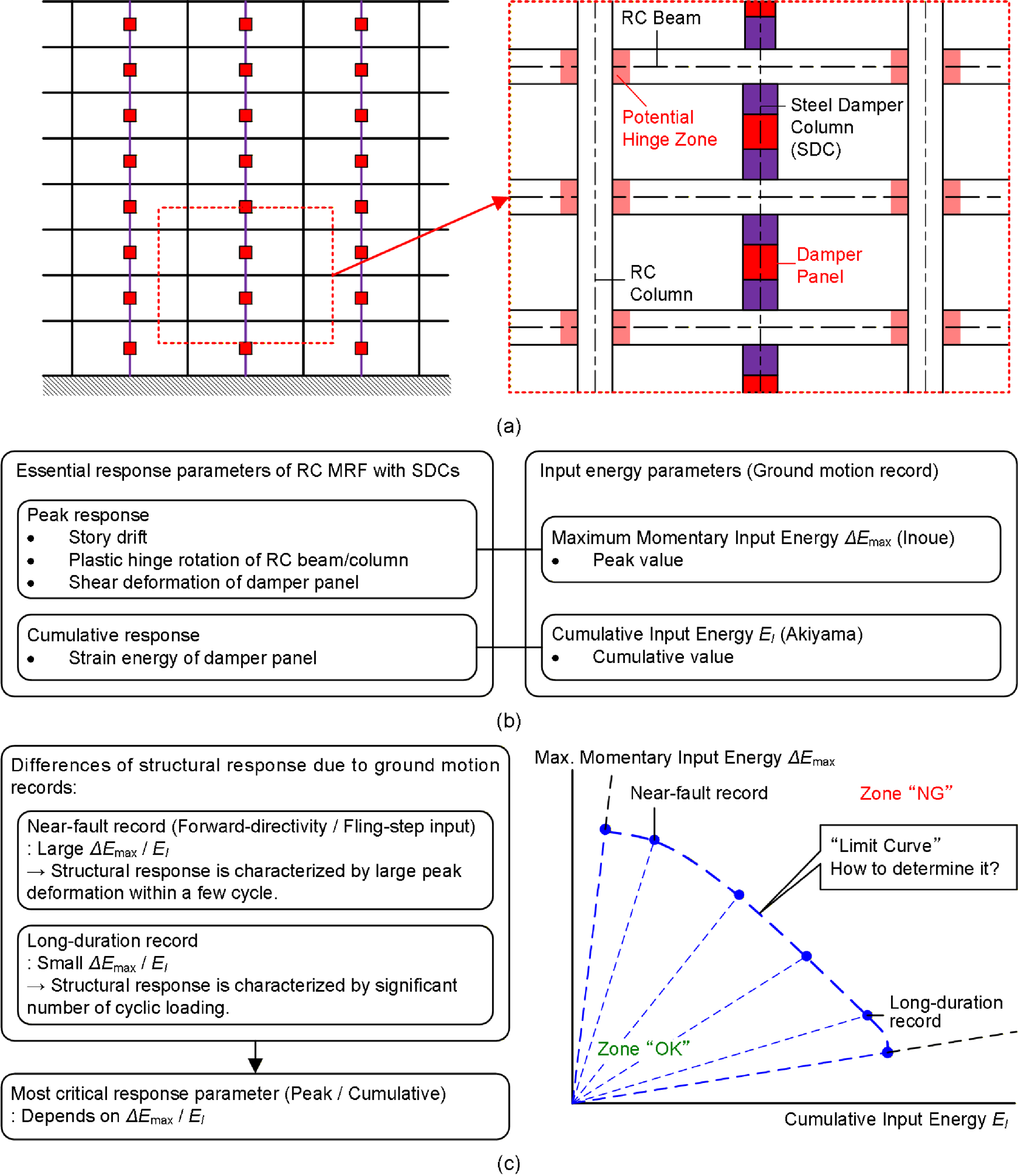
Figure 2.
Building Model (Fujii, 2025b). (a) structural plan (Dp033), (b) structural plan (Dp050), (c) structural plan (Dp100), (d) structural model of frame A (Dp050), (e) structural model of frame A (Dp100).
Figure 2.
Building Model (Fujii, 2025b). (a) structural plan (Dp033), (b) structural plan (Dp050), (c) structural plan (Dp100), (d) structural model of frame A (Dp050), (e) structural model of frame A (Dp100).
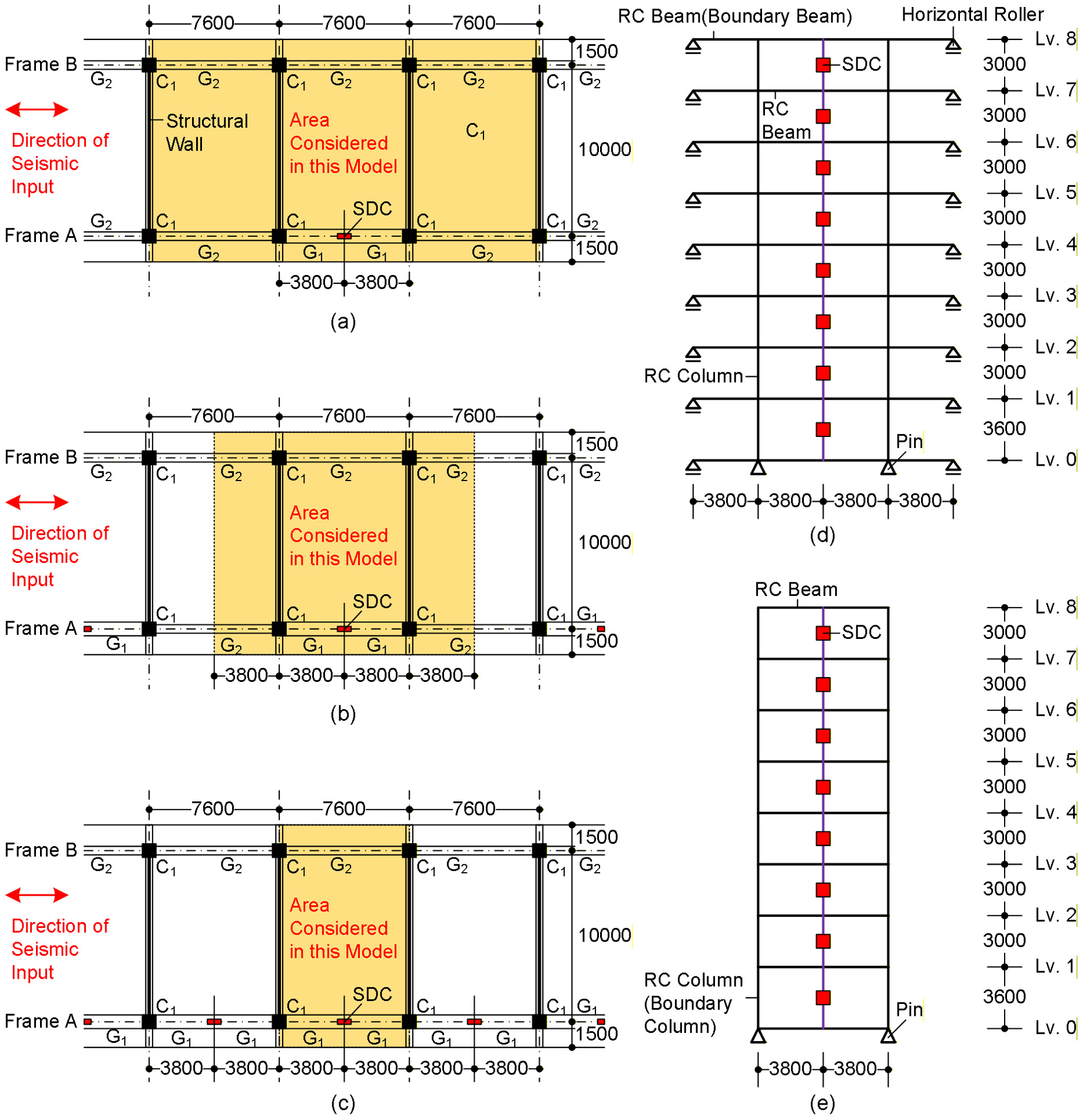
Figure 3.
Hysteresis model. (a) RC members, (b) damper panel (SDC). Note that this figure is reproduced by modifying from Fujii (2024b).
Figure 3.
Hysteresis model. (a) RC members, (b) damper panel (SDC). Note that this figure is reproduced by modifying from Fujii (2024b).
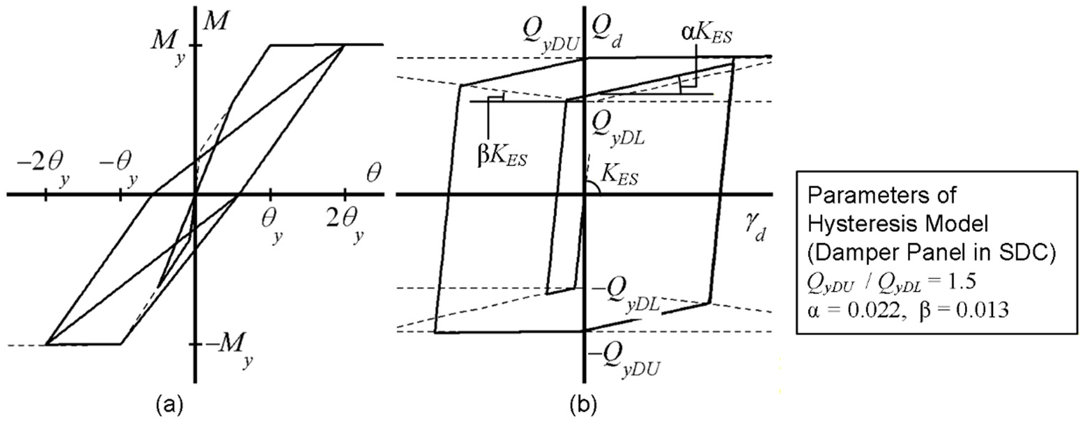
Figure 4.
Response limit of a damper panel in SDC applied in this study and accuracy of the hysteresis model of damper panel. (a) response limit of a damper panel applied in this study (JFE Civil, 2025), (b) history of shear strain in the test (24DC42), (c) history of the normalized cumulative strain energy of damper panel, (d) hysteresis loop of damper panel, (e) comparisons of the normalized dissipated energy per one cycle. Note that the plots of 24DC42 and the horizontal dashed line (Δγdlimit = 0.1) in the right panel of Figure 4a are added by the author.
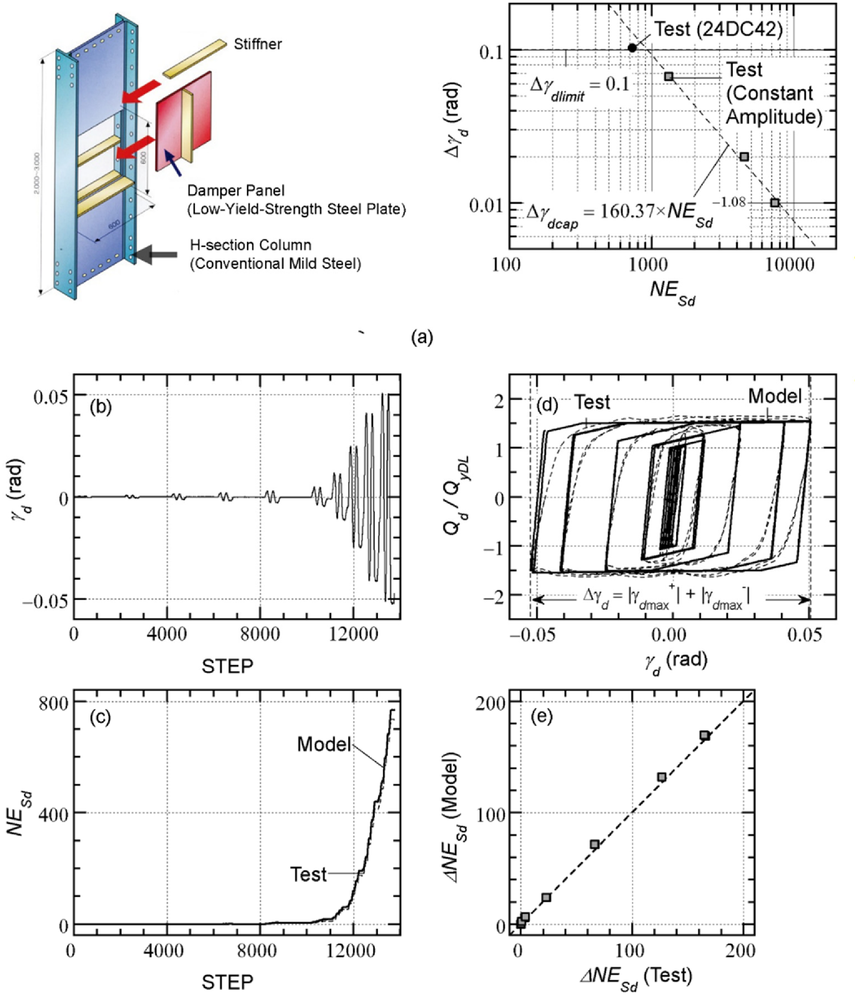
Figure 5.
Time-history of the critical PMI analysis results (Dp100, Vp = 0.763 m/s, Np = 4). (a) input energy per unit mass of the first modal response, (b) equivalent displacement of the first modal response, (c) story drift at the second story, (d) shear strain of damper panel in SDC at the second story, (e) normalized cumulative strain energy of damper panel in SDC at the second story, (f) hysteresis loop of the first modal response, (g) hysteresis loop of the damper panel in SDC at the second story.
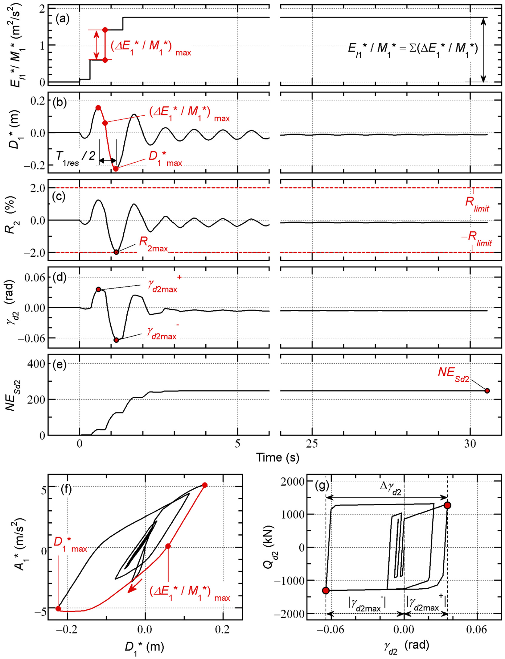
Figure 6.
Response profiles obtained from the ICPMIA results (Dp100). (a) R2max - Vp relationship, (b) Δγd2 - Vp relationship, (c) NESd2 - Vp relationship, (d) Δγd2 - NESd2 relationship, (e) (D/C)2 - Vp relationship, (f) T1res - Vp relationship.
Figure 6.
Response profiles obtained from the ICPMIA results (Dp100). (a) R2max - Vp relationship, (b) Δγd2 - Vp relationship, (c) NESd2 - Vp relationship, (d) Δγd2 - NESd2 relationship, (e) (D/C)2 - Vp relationship, (f) T1res - Vp relationship.
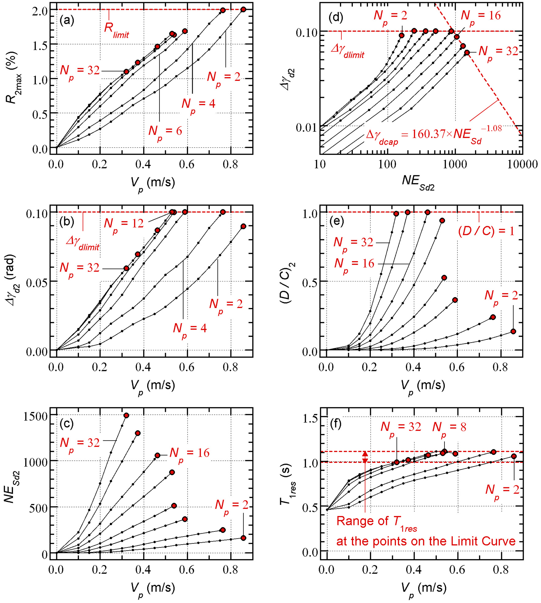
Figure 7.
Energy-based limit curve from obtained ICPMIA results (Dp100). (a) VΔE1* - Vp relationship, (b) VI1* - Vp relationship, (c) VΔE1*/VI1* - Vp relationship, (d) VΔE1* - VI1* relationship (limit curve).
Figure 7.
Energy-based limit curve from obtained ICPMIA results (Dp100). (a) VΔE1* - Vp relationship, (b) VI1* - Vp relationship, (c) VΔE1*/VI1* - Vp relationship, (d) VΔE1* - VI1* relationship (limit curve).
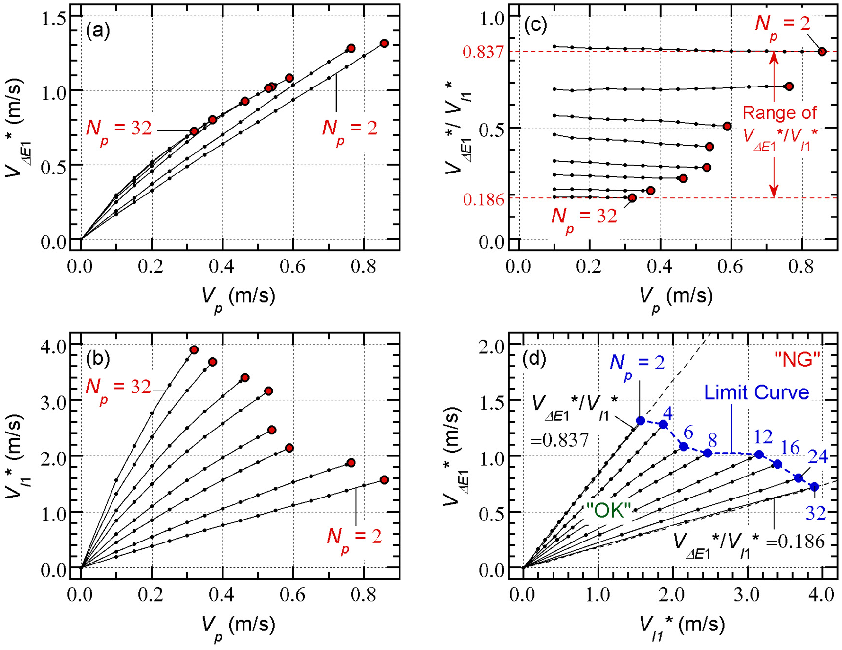
Figure 8.
Comparisons of the limit curve of models.
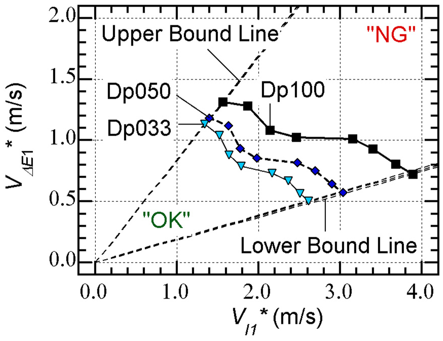
Figure 9.
Energy spectrum of ground motion records. (a) IWN-NS, (b) UTO-NS.
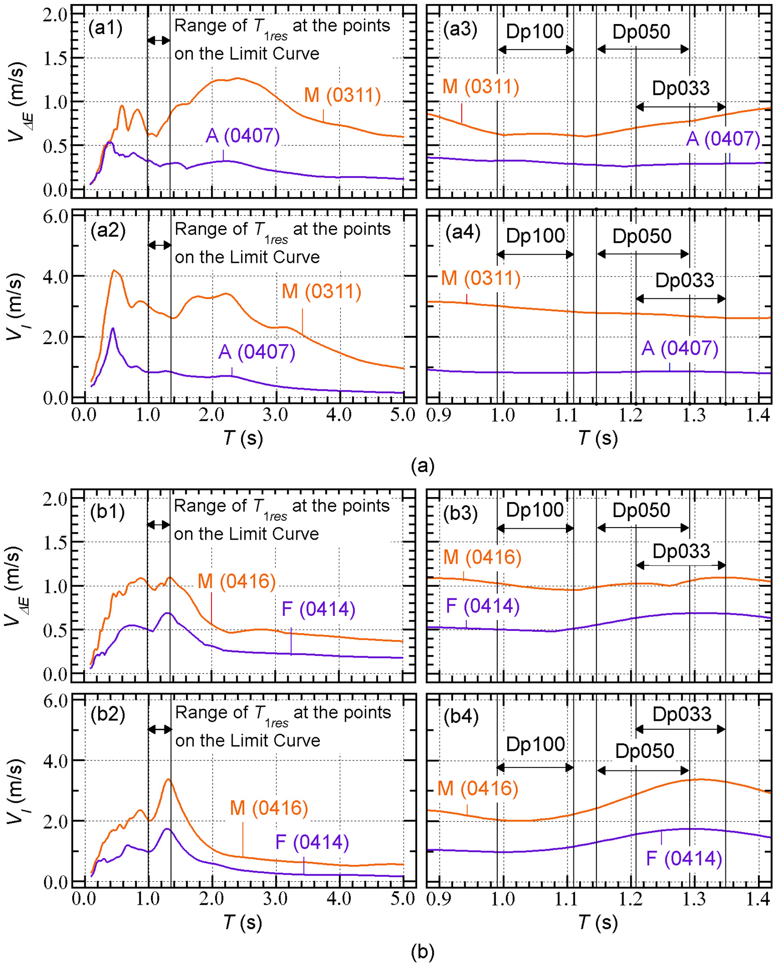
Figure 10.
Response profiles of models (IWN-NS). (a) Dp033, (b) Dp050, (c) Dp100.
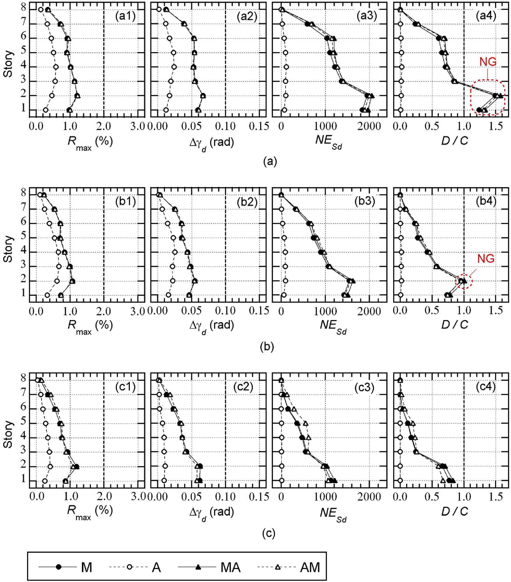
Figure 11.
Response profiles of models (UTO-NS). (a) Dp033, (b) Dp050, (c) Dp100.
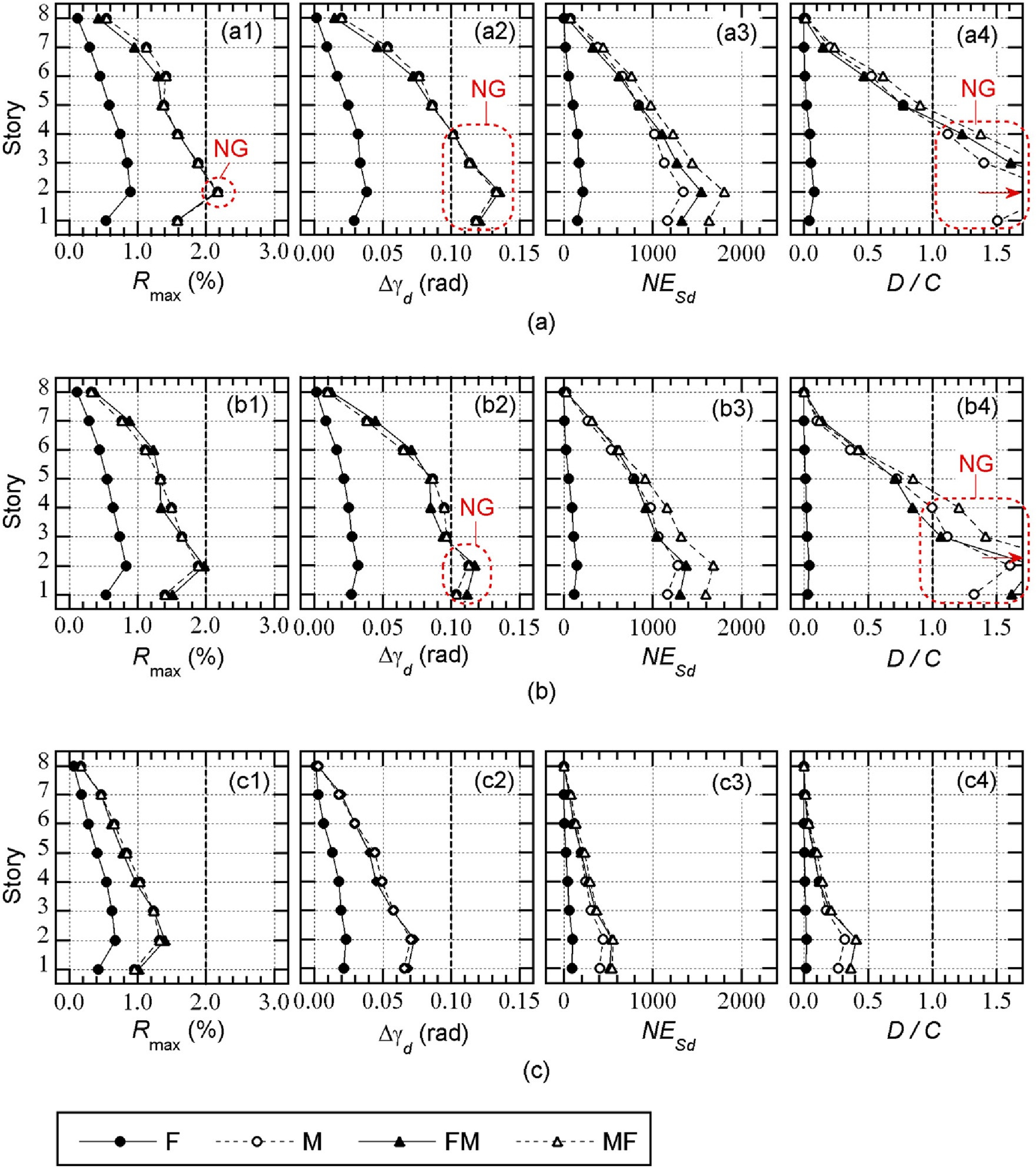
Figure 12.
Comparisons with the limit curve and earthquake responses. (a) Dp033, (b) Dp050, (c) Dp100.
Figure 12.
Comparisons with the limit curve and earthquake responses. (a) Dp033, (b) Dp050, (c) Dp100.
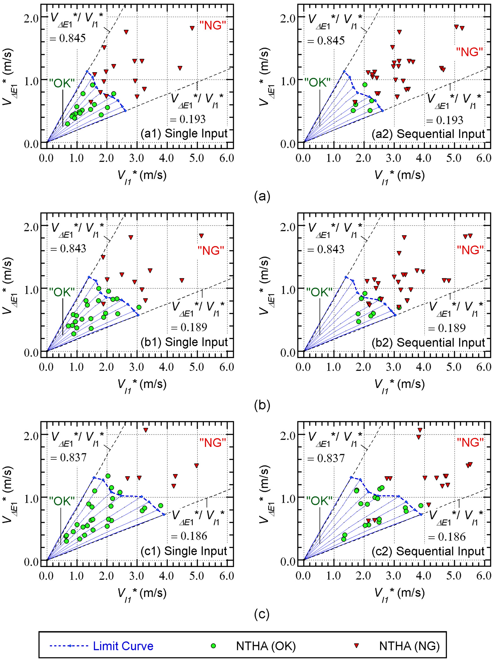

Table 1.
List of ground motion records.
| Station Name | Event Date | Distance (km) | Ground Motion ID | PGA (m/s2) |
|---|---|---|---|---|
| K-NET Tsukidate (MYG004) |
11 March 2011 | 175 | TSK-EW(M) | 12.69 |
| TSK-NS(M) | 27.00 | |||
| 07 April 2011 | 98 | TSK-EW(A) | 8.86 | |
| TSK-NS(A) | 12.42 | |||
| K-NET Furukawa (MYG006) |
11 March 2011 | 174 | FRK-EW(M) | 5.72 |
| FRK-NS(M) | 4.44 | |||
| 07 April 2011 | 93 | FRK-EW(A) | 4.79 | |
| FRK-NS(A) | 4.16 | |||
| K-NET Shiogama (MYG012) |
11 March 2011 | 163 | SGM-EW(M) | 19.69 |
| SGM-NS(M) | 7.58 | |||
| 07 April 2011 | 80 | SGM-EW(A) | 14.47 | |
| SGM-NS(A) | 5.56 | |||
| K-NET Sendai (MYG013) |
11 March 2011 | 170 | SND-EW(M) | 9.82 |
| SND-NS(M) | 15.17 | |||
| 07 April 2011 | 87 | SND-EW(A) | 10.02 | |
| SND-NS(A) | 5.89 | |||
| K-NET Iwanuma (MYG015) |
11 March 2011 | 174 | IWN-EW(M) | 3.53 |
| IWN-NS(M) | 4.11 | |||
| 07 April 2011 | 93 | IWN-EW(A) | 3.94 | |
| IWN-NS(A) | 3.43 | |||
| K-NET Kumamoto (KMM006) |
14 April 2016 | 6 | KMM-EW(F) | 3.81 |
| KMM-NS(F) | 5.74 | |||
| 16 April 2016 | 5 | KMM-EW(M) | 6.16 | |
| KMM-NS(M) | 8.27 | |||
| K-NET Uto (KMM008) |
14 April 2016 | 15 | UTO-EW(F) | 3.04 |
| UTO-NS(F) | 2.64 | |||
| 16 April 2016 | 12 | UTO-EW(M) | 7.71 | |
| UTO-NS(M) | 6.52 | |||
| KIK-NET Mashiki (KMMH16) |
14 April 2016 | 6 | MAS-EW(F) | 9.25 |
| MAS-NS(F) | 7.60 | |||
| 16 April 2016 | 7 | MAS-EW(M) | 11.57 | |
| MAS-NS(M) | 6.53 |
Table 2.
Validation results of limit curve.
| Model | Input type | Total cases | Agreements | Agreement ratio |
|---|---|---|---|---|
| Dp033 | Single | 32 | 28 | 87.5% |
| Dp050 | 29 | 90.6% | ||
| Dp100 | 28 | 87.5% | ||
| Dp033 | Sequential | 29 | 90.6% | |
| Dp050 | 27 | 84.4% | ||
| Dp100 | 27 | 84.4% |
Disclaimer/Publisher’s Note: The statements, opinions and data contained in all publications are solely those of the individual author(s) and contributor(s) and not of MDPI and/or the editor(s). MDPI and/or the editor(s) disclaim responsibility for any injury to people or property resulting from any ideas, methods, instructions or products referred to in the content. |
© 2026 by the authors. Licensee MDPI, Basel, Switzerland. This article is an open access article distributed under the terms and conditions of the Creative Commons Attribution (CC BY) license (http://creativecommons.org/licenses/by/4.0/).
Copyright: This open access article is published under a Creative Commons CC BY 4.0 license, which permit the free download, distribution, and reuse, provided that the author and preprint are cited in any reuse.


