
Submitted:
09 January 2026
Posted:
09 January 2026
You are already at the latest version
Abstract
We have collected geomagnetic observations from low and equatorial latitudes during the 19th century to infer the intensity of geomagnetic storms during the years 1841-1877. Daily mean H observations during the above years in Trivandrum, Singapore and Madras is first scaled to Bombay observations and subsequently to the Dst index to infer the intensity of storms in modern units . These results are also compared with the intensity of these storms derived from mid latitudes. Extreme space weather events (ESW) are identified from the list of intense storms inferred during this period. The annual number of ESW events shows the characteristic double peak structure during the sunspot cycles 9-11. Space weather conditions during the sunspot cycle 11 (1867-1877) is found to be exceptional. A discussion on the true intensity of geomagnetic storms is also included.
Keywords:
geomagnetic storms
; 19th century
; Trivandrum
; Singapore
; Madras
; space weather
1. Introduction
Geomagnetic storms are important manifestations of space weather changes near Earth (Mandea and Chemboldt, 2021.) The severity of space weather conditions generally increase with the intensity of these storms. Direct records of extreme space weather events dates back to middle of the 19th century ( Cliver and Svaalgaard,2004 and the pr)oxy records of the same is available back to the 16th century ( Cliver et al., 2022). The intensity of geomagnetic storms is related to the strength of the magnetospheric ring current whose effects are prominent in both low and equatorial magnetic latitudes in Earth (Ganuskina et al., 2017). Both Dst and Sym H indices are now used to determine intensity of geomagnetic storms (Villaverde etal, 2024). Dst index is currently derived from H variations in four low latitude stations after making necessary Sq corrections. ( Geomagnetic Equatorial Dst index, available in : https://wdc.kugi.kyoto-u.ac.jp/dstdir/ ) Records of mid latitude geomagnetic observations are well documented and dates back to the19th century ( Jones, 1955; Stamper et al., 1999;Nevanlinna, 2004).This is not however true for observations from low and equatorial magnetic latitudes.
Systematic and long term geomagnetic observations started for the first time in the Greenwitch observatory in London during the year 1840. Magnetic observations in British colonies were coordinated by the Royal Society of London during the 1840’s . It is quiet interesting to find that magnetic observatories were established in Singapore, Trivandrum and Madras during the year 1841. Continuous geomagnetic observations started in Colaba observatory in Bombay ( now Mumbai ) began later from the year 1846 onwards ( Moos, 1910 a).Magnetic observations in these observatories were carried out following the standards and instructions of the royal society ( Royal Society, 1840).Only part of the 19th century magnetic observations in the above colonial observatories were either studied or published. Rest of them is possibly available in manuscript form in different archives of the world.
The observatories covered in this chapter are mainly low or equatorial latitude observatories which were functioning at Trivandrum, Madras, Bombay and Singapore during the British administration periods. Early geomagnetic observations made in these observatories are by and large hourly eye readings of different magnetic elements which can be reduced to old British geomagnetic units ( and further to SI units) if the constants of measurements are known.There are several challenges in analysing geomagnetic data during the 19th century ( Blake etal, 2020; Hejda et al., 2023). In order to study hourly H observations of that period we should know i) the type of bifilar magnetometer used for H measurements ii) the magnetometer constants ( unit or scale coefficient and temperature coefficient ) which will vary from time to time and iii) absolute measurements of H ( at least on monthly or yearly basis) in that observatory ( Broun, 1862). These details are studied in detail for the daily mean H observations from the Trivandrum observatory during the years 1855-1877.
In this paper using daily mean H observations in Singapore ( 1841-1845), Madras ( 1846-1855) and Trivandrum ( 1855-1877) we have attempted to infer the intensity of major geomagnetic storms during the years 1841-1877. Intensity of the storms are( in units of nT) are initially determined by scaling with Bombay H observations. Subsequently intensity of storms ( in units of nT) are scaled to Dst values using the Carrington storm observations a reference. The results are then compared with We have identified occurrences of extreme space weather events ( ESW) during the years 1841-1877 from the list of extreme intense and super intense storms inferred during this period . Annual number of ESW events show characteristic solar cycle variations during the sunspot cycles 9-11. Exceptional space weather activity during solar cycle 11 ( 1867-1877) is a new result from this study. After pointing out the limitations in the modern Dst index the need for determining true intensity of geomagnetic storms are also discussed.
2. Details of Data Used
2.1 Published values of daily mean horizontal intensity ( H) of geomagnetic ( as ratio relative to absolute H ) of the Singapore magnetic observatory ( ref) during years 1841-1845 ( Eliot, 1850)
2.2 Published values of daily mean horizontal intensity ( H) of geomagnetic ( as ratio relative to absolute H ) of the Madras magnetic observatory ( ref) during years 1846-1855 ( Taylor et al., 1854; Jacob, 1884)
2.3 (a) Geomagnetic storm intensity derived for selected list of geomagnetic storms during 1852-63 adopted from Table of the PhD thesis ( Eapen, 2009) using published hourly values of H ( in British units) from Bombay ( Colaba) observatory during the years 1852-1863 ( Chambers, 1852; Fergusson, 1860 etc )
(b) Selected values of storm decrease in hourly values of H in Bombay( Colaba ) observatory during the years 1847-1877 ( Lakhina and Tsuratani, 2018; Kumar et al., 2015; Moos, 2010b).
2.4 Daily mean H values in Trivandrum magnetic observatory ( in scale divisions) obtained in manuscript form from National Library of Scotland during the years 1855-1877. ( NLS, 2007a; NLS, 2007b).
2.5 International yearly mean Sunspot number ( classic values ) during the years 1841-1877 ( available in : https://www.sws.bom.gov.au/Educational/2/3/6).
2.6 Geomagnetic storm data from the Greenwitch observatory during the years 1841-1877 ( Jones, 1955; Maunder, 1905; Airy, 1863).
2.7 Geomagnetic storm data from Russian magnetic observatories during the years ( Ptisyna et al., 2012).
2.8 (a) 3 hourly aa indices during the years 1868-1877 and
(b) Yearly mean aa indices during the years 1868-1877 ( available in https://www.ngdc.noaa.gov/stp/space-weather/geomagnetic-data/AA_INDEX/AA_YEAR )
2.9 Information on extreme space weather events during 1841-2024 from different publications ( Cliver and Svaalgaard, 2004; Cliver et al., 2022; Vennerstorm et al., 2010; Rao, 1964; Tulasi Ram et al., 2024).
3. Investigations on the Geomagnetic Observations in Low/Equitorial Latitudes During the Years 1841-1877
3.1. Bombay Geomagnetic Observations and Storm Intensity Calculations During 1852-1863
Even though Coloba ( Bombay) magnetic observatory is established during the year 1841 regular observations were started only from the year 1845 ( Gawali et al., 2015) Eye readings of geomagnetic elements continued till the year 1872 when photographic recordings were started ( Moos, 1910a). Horizontal intensity is measured mainly with large horizontal force magnetometer with bifilar suspension whose details are available in early data books of the observatory ( Chambers, 1852 etc)
Hourly values of horizontal component of the geomagnetic field (H) observed in Coloba observatory in Bombay ( now Mumbai) is collected for selected geomagnetic storm periods during 1852-1863. This data is available in British units ( BU) of intensity. The intensity of major geomagnetic storms observed in Bombay in modern units during the years 1852-63 is available in Eapen ( 2009). Let is discuss some examples in this list :-
First we will consider the intensity calculations for two outstanding geomagnetic storms during the period of study. For the Carrington storm of September 2, 1859 (Fergusson, 1860; see also Figure 1 in Hayakawa et al., 2022) the pre-storm maximum or baseline in hourly H of Colaba is found to be 8.0467 BU. The storm time minimum in Colaba H during September 2, 1859 is found to be 7.672 BU. The difference between the two values is ΔH (= 0.3747 BU) or decrease in H during the main phase the Carrington stoof rm. To convert in to modern units we will use the following expression (Chapman and Gupta, 1971; Eapen, 2009)
ΔH(nT) = ΔH( (BU) x 36000 / 7.8 (1)
For the Carrington storm we could find from (1)
ΔH (Colaba) = 1729.38 nT (2)
For the October 12, 1859 storm we have found
ΔH (Colaba) = 0.2097 BU = 967.85 nT (3)
The values of ΔH for Colaba observatory published by Lakhina and Tsurutani ( 2018) for the Carrington storm is 1722 nT and for the October 12 ( 1859) storm is 984 nT. This justifies our calculations for the above two outstanding storms for Bombay. In a similar way we have calculated the intensity (ΔH) for more than 30 geomagnetic storms in Bombay during the years 1852-1863. The results are given in Table 2 and Table 5..
3.2 Madras Geomagnetic Observations and Storm Intensity Calculations
Earliest geomagnetic observations in Madras are made by TG Taylor ( Govt Astronomer , Madras Observatory) along with John Caldecott ( Director, Trivandrum Observatory) during 1837-38 period as a part of the magnetic survey of South India (Taylor, 1837;Taylor and Caldecott, 1839). The geographic coordinates of Madras is found ( Taylor and Caldecott, 1839) to be 130 4’ 9” N latitude and 800 17’ 12” E longitude.The magnetic dip of Madras is determined as 60 50’ 9” ( north of dip equator) in 1838. The mean magnetic dip of Madras during January 1851 was 70 37’ 15” which increased to 70 39’3” during December 1855. The absolute horizontal intensity (H) of earths magnetic field measured in Madras varied between 8.1606 to 8.1970 BU during January 1851 and between 8.0682 to 8.1324 BU during December 1855.
Capt Ludlow ( Madras Engineers) started geomagnetic observations in Madras Observatory
during March 1841. Observations during 1841-1845 and 1856-61 are not published so far and is believed to be available in hidden archives in manuscript form in London. Madras geomagnetic observations during 1846-1850 ( Taylor et al., 1854) and 1851-1855 ( Jacob, 1884) are however published . These later observations are used for the present study. The horizontal intensity data of Madras are given in these publications as hourly eye readings. This needs to be corrected for atmospheric temperature variations and required conversion in to relative intensity or British units which is not straight forward. However temperature corrected mean daily values of H in relative intensity values ( as a fraction of the absolute H in Madras ) are however available. We have used these values to determine the H decreases (ΔH ) during magnetic storms in Madras during the years 1846-1855. Mean H values of Madras ( in relative intensity units) given in the data books during February 1852 is shown in Figure 1. The MDS Hd in relative units for this storm is found to be 0.00452 . As an approximation we can assume 8.1 BU is the mean absolute H in Madras during our period of study so that for the February 18-19 storm of 1852 we have :
MDS Hd (BU) = MDS Hd X 8.1 = 0.00452 X 8.1 =0.03661 BU (4)
We have identified important geomagnetic storms during 1846-1855 using published Greenwich geomagnetic results (ref) . For each of these storm periods we have determined MDS Hd in BU using (4) These results are shown in Table 1 and Table 2
. In order to find the intensity of the storms in terms of modern units we have done a linear regression fit of MDS Hd (BU) values of Madras ( 1852-1855) with corresponding ΔH ( hourly) values from Bombay observations (see Table ) , The results are shown in Figure 2.
The yields the following linear regression equation :.
MDS ΔH (nT) = 7315.8 Hd (BU) +91.569 ( R2 = 0.6483, r = 0.81) (5)
Here MDS ΔH is the magnitude of storm time decrease in Madras scaled to Bombay observations in modern units (nT) and Hd is the observed magnitude of storm time decrease in Madras in BU .
Using (5) we have determined ΔH (nT) of Madras storms in modern units during the years 1846-1855. The results are shown in Table 1 and Table 2. The Greenwich classification of intense ( A) and Great storms (G) are also included in these Tables ( Maunder, 1905; Jones, 1955).

Table 1.
Geomagnetic storm parameters in Madras Observatory during the years 1846-1851.
| Sr No | Year | Storm Date |
GW Class | MDS Hd |
MDS Hd (BU) |
MDS ΔH (nT) |
Tvm Dst ( nT) |
|---|---|---|---|---|---|---|---|
| 1 | 1846 | 24-Jan | 0.000489 | 0.0039609 | 120.54 | 105.9056221 | |
| 2 | 1846 | 9-Feb | 0.001072 | 0.0086832 | 155.0945546 | 176.1215008 | |
| 3 | 1846 | 13-Mar | 0.001795 | 0.0145395 | 197.9380741 | 263.1988255 | |
| 4 | 1846 | 6-Apr | 0.002101 | 0.0170181 | 216.071016 | 300.0531289 | |
| 5 | 1846 | 7-Apr | 0.001503 | 0.0121743 | 180.6347439 | 228.0306667 | |
| 6 | 1846 | 12-May | 0.00162 | 0.013122 | 187.5679276 | 242.122018 | |
| 7 | 1846 | 11-Jul | 0.000678 | 0.0054918 | 131.7469104 | 128.6685742 | |
| 8 | 1846 | 7-Aug | 0.001357 | 0.0109917 | 171.9830789 | 210.4465873 | |
| 9 | 1846 | 4-Sep | 0.001161 | 0.0094041 | 160.3685148 | 186.8405629 | |
| 10 | 1846 | 11-Sep | 0.001226 | 0.0099306 | 164.2202835 | 194.6690914 | |
| 11 | 1846 | 22-Sep | G | 0.000541 | 0.0043821 | 123.6285672 | 112.1684449 |
| 12 | 1846 | 8-Oct | 0.000624 | 0.00505359 | 128.5410537 | 122.1528297 | |
| 13 | 1846 | 17-Nov | 0.001832 | 0.0148392 | 200.1306194 | 267.6550648 | |
| 14 | 1846 | 26-Nov | 0.001408 | 0.0114048 | 175.0052358 | 216.5889712 | |
| 15 | 1846 | 23-Dec | 0.00084 | 0.006804 | 141.3467032 | 148.179676 | |
| 16 | 1847 | 22-Feb | 0.001904 | 0.0154224 | 204.3971939 | 276.3266656 | |
| 17 | 1847 | 1-Mar | 0.001948 | 0.0157788 | 207.004545 | 281.6259772 | |
| 18 | 1847 | 19-Mar | G | 0.00364 | 0.029484 | 307.2690472 | 485.408596 |
| 19 | 1847 | 8-Apr | 0.002145 | 0.0173745 | 218.6783671 | 305.3524405 | |
| 20 | 1847 | 21-Apr | 0.002932 | 0.0237492 | 265.3143974 | 400.1378548 | |
| 21 | 1847 | 8-May | 0.002313 | 0.0187353 | 228.6337077 | 325.5861757 | |
| 22 | 1847 | 10-Jul | 0.001306 | 0.0105786 | 168.9609219 | 204.3042034 | |
| 23 | 1847 | 24-Sep | G | 0.005122 | 0.0414882 | 395.0893736 | 663.8990458 |
| 24 | 1847 | 27-Sep | 0.003436 | 0.0278316 | 295.1804193 | 460.8390604 | |
| 25 | 1847 | 1-Nov | 0.004743 | 0.0384183 | 372.6305991 | 618.2527027 | |
| 26 | 1847 | 23-Nov | 0.000515 | 0.0041715 | 122.0878597 | 109.0370335 | |
| 27 | 1847 | 17-Dec | G | 0.000116 | 0.0009396 | 98.44392568 | 60.9819124 |
| 28 | 1847 | 20-Dec | G | 0.005587 | 0.0452547 | 422.6443343 | 719.9031343 |
| 29 | 1848 | 12-Jan | 0.001115 | 0.0090315 | 157.6426477 | 181.3003735 | |
| 30 | 1848 | 21-Feb | G | 0.003551 | 0.0287631 | 301.995087 | 474.6895339 |
| Sr No | Year |
Storm Date |
GW Class |
MDS Hd |
MDS Hd (BU) |
MDS ΔH (nT) |
Tvm Dst ( nT) |
| 31 | 1848 | 20-Mar | A | 0.002659 | 0.0215379 | 249.1369688 | 367.2580351 |
| 32 | 1848 | 25-Mar | 0.001004 | 0.0081324 | 151.0650119 | 167.9316556 | |
| 33 | 1848 | 16-Apr | A | 0.001416 | 0.0114696 | 175.4792997 | 217.5524824 |
| 34 | 1848 | 11-Jul | A | 0.002737 | 0.0221697 | 253.7590913 | 376.6522693 |
| 35 | 1848 | 23-Oct | A | 0.002384 | 0.0193104 | 232.8410243 | 334.1373376 |
| 36 | 1848 | 17-Nov | G | 0.005241 | 0.0424521 | 402.1410732 | 678.2312749 |
| 37 | 1849 | 30-Jan | 0.000903 | 0.0073143 | 145.0799559 | 155.7673267 | |
| 38 | 1849 | 13-Sep | 0.000836 | 0.0067716 | 141.1096713 | 147.6979204 | |
| 39 | 1849 | 31-Oct | A | 0.000926 | 0.0075006 | 146.4428895 | 158.5374214 |
| 40 | 1849 | 13-Nov | 0.001035 | 0.0083835 | 152.9020093 | 171.6652615 | |
| 41 | 1849 | 29-Nov | A | 0.001713 | 0.0138753 | 193.0789197 | 253.3228357 |
| 42 | 1850 | 22-Feb | A | 0.001646 | 0.0133326 | 189.1086351 | 245.2534294 |
| 43 | 1850 | 11-Mar | 0.00091 | 0.007371 | 145.4947618 | 156.610399 | |
| 44 | 1850 | 25-Mar | 0.001555 | 0.0125955 | 183.7161589 | 234.2934895 | |
| 45 | 1850 | 4-May | 0.00067 | 0.005427 | 131.2728466 | 127.705063 | |
| 46 | 1850 | 2-Jul | 0.000786 | 0.0063666 | 138.1467723 | 141.6759754 | |
| 47 | 1850 | 1-Oct | 0.002151 | 0.0174231 | 219.033915 | 306.0750739 | |
| 48 | 1850 | 17-Dec | 0.001588 | 0.0128628 | 185.6716722 | 238.2679732 | |
| 49 | 1850 | 27-Dec | 0.000976 | 0.0079056 | 149.4057885 | 164.5593664 | |
| 50 | 1851 | 20-Jan | A | 0.002813 | 0.0227853 | 258.2626977 | 385.8056257 |
| 51 | 1851 | 6-Feb | 0.000637 | 0.0051597 | 129.3173333 | 123.7305793 | |
| 52 | 1851 | 19-Feb | A | 0.001762 | 0.0142722 | 195.9825608 | 259.2243418 |
| 53 | 1851 | 24-Aug | A | 0.001116 | 0.0090396 | 157.7019057 | 181.4208124 |
| 54 | 1851 | 3-Sep | A | 0.001297 | 0.0105057 | 168.4276001 | 203.2202533 |
| 55 | 1851 | 29-Sep | G | 0.00247 | 0.020007 | 237.9372106 | 344.495083 |
| 56 | 1851 | 3-Oct | G | 0.001298 | 0.0105138 | 168.486858 | 203.3406922 |
| 57 | 1851 | 28-Oct | A | 0.001008 | 0.0081648 | 151.3020438 | 168.4134112 |
| 58 | 1851 | 8-Dec | G | 0.001033 | 0.0083673 | 152.7834933 | 171.4243837 |
| 59 | 1851 | 28-Dec | A | 0.001545 | 0.0125145 | 183.1235791 | 233.0891005 |
Table 2.
Geomagnetic storm parameters in Madras and Bombay Observatory during 1852-1855.
| Sr No | Year | Storm Date |
GW class |
MDS Hd |
MDS Hd (BU) |
MDS ΔH (nT) |
Bom ΔH (nT) |
Tvm Dst (nT) |
|---|---|---|---|---|---|---|---|---|
| 1 | 1852 | 7-Jan | 0.000397 | 0.003216 | 115.0954 | 94.82524 | ||
| 2 | 1852 | 20-Jan | A | 0.001389 | 0.011251 | 173.8793 | 164.77 | 214.3006 |
| 3 | 1852 | Feb 18,19 | G | 0.00452 | 0.036612 | 359.4161 | 1575 | 591.3948 |
| 4 | 1852 | 7-Mar | 0.000678 | 0.005492 | 131.7469 | 108.46 | 128.6686 | |
| 5 | 1852 | 12-Mar | 0.000992 | 0.008035 | 150.3539 | 166.4864 | ||
| 6 | 1852 | 26-Mar | A | 0.000455 | 0.003686 | 118.5324 | 101.8107 | |
| 7 | 1852 | 21-Apr | A | 0.002066 | 0.016735 | 213.997 | 228.92 | 295.8378 |
| 8 | 1852 | 2-May | 0.001033 | 0.008367 | 152.7835 | 171.4244 | ||
| 9 | 1852 | 20-May | 110.77 | |||||
| 10 | 1852 | 27-May | A | 0.00119 | 0.009639 | 162.087 | 190.3333 | |
| 11 | 1852 | Jun 11,12 | A | 0.001644 | 0.013316 | 188.9901 | 245.0126 | |
| 12 | 1852 | Jun,17,18 | A | 0.001322 | 0.010708 | 169.909 | 206.2312 | |
| 13 | 1852 | Jul,10 | 0.000852 | 0.006901 | 142.0578 | 149.6249 | ||
| 14 | 1852 | Aug 10,11 | 0.000413 | 0.003345 | 116.0435 | 96.75227 | ||
| 15 | 1852 | 24-Aug | 0.000793 | 0.006423 | 138.5616 | 134.31 | 142.519 | |
| 16 | 1852 | 9-Sep | 0.000546 | 0.004423 | 123.9249 | 112.15 | 112.7706 | |
| 17 | 1852 | 22-Sep | 85.85 | |||||
| 18 | 1852 | 29-Sep | 0.000555 | 0.004496 | 124.4582 | 113.8546 | ||
| 19 | 1852 | Oct 18,19 | 0.001017 | 0.008238 | 151.8354 | 116.31 | 169.4974 | |
| 20 | 1852 | 12-Nov | G | 0.001049 | 0.008497 | 153.7316 | 186 | 173.3514 |
| 21 | 1852 | 11-Dec | 142.62 | |||||
| 22 | 1852 | 29-Dec | 0.001065 | 0.008627 | 154.6797 | 175.2784 | ||
| 23 | 1853 | Jan 9,10 | 0.000892 | 0.007225 | 144.4281 | 154.4425 | ||
| 24 | 1853 | 14-Feb | 0.001975 | 0.015998 | 208.6045 | 169.85 | 284.8778 | |
| 25 | 1853 | 21-Feb | 0.001677 | 0.013584 | 190.9456 | 248.987 | ||
| 26 | 1853 | 8-Mar | 0.001017 | 0.008238 | 151.8354 | 169.4974 | ||
| 27 | 1853 | Apr 5,6 | 0.001479 | 0.01198 | 179.2126 | 225.1401 | ||
| 28 | 1853 | 3-May | 0.001487 | 0.012045 | 179.6866 | 226.1036 | ||
| 29 | 1853 | 24-May | A | 0.00181 | 0.014661 | 198.8269 | 192 | 265.0054 |
| 30 | 1853 | 2-Jun | 0.001364 | 0.011048 | 172.3979 | 211.2897 | ||
| 31 | 1853 | 22-Jun | A | 0.000454 | 0.003677 | 118.4731 | 101.6903 | |
| 32 | 1853 | 12-Jul | G | 0.001182 | 0.009574 | 161.6129 | 189.3698 | |
| 33 | 1853 | 26-Aug | 0.000463 | 0.00375 | 119.0064 | 102.7742 | ||
| 34 | 1853 | 2-Sep | A | 0.001769 | 0.014329 | 196.3974 | 175.38 | 260.0674 |
| 35 | 1853 | 27-Sep | 170.77 | |||||
| Sr No | Year |
Storm Date |
GW class |
MDS Hd |
MDS Hd (BU) |
MDS ΔH (nT) |
Bom ΔH (nT) |
Tvm Dst (nT) |
| 36 | 1853 | 15-Oct | 0.000711 | 0.005759 | 133.7024 | 132.6431 | ||
| 37 | 1853 | 31-Oct | 0.001652 | 0.013381 | 189.4642 | 245.9761 | ||
| 38 | 1853 | 9-Nov | A | 0.001338 | 0.010838 | 170.8572 | 208.1582 | |
| 39 | 1853 | 6-Dec | A | 0.002437 | 0.01974 | 235.9817 | 248.31 | 340.5206 |
| 40 | 1853 | 21-Dec | A | 0.000669 | 0.005415 | 131.1875 | 127.5316 | |
| 41 | 1854 | Jan 2,3 | 0.001794 | 0.014531 | 197.8788 | 146.31 | 263.0784 | |
| 42 | 1854 | Jan 8,9 | 0.000282 | 0.002284 | 108.2808 | 80.97477 | ||
| 43 | 1854 | 20-Jan | 0.000438 | 0.003548 | 117.525 | 99.76324 | ||
| 44 | 1854 | 29-Jan | -8.6E-05 | -0.0007 | 86.47381 | 36.65325 | ||
| 45 | 1854 | 11-Feb | 0.001388 | 0.011243 | 173.8201 | 214.1802 | ||
| 46 | 1854 | 16-Feb | A | 0.001057 | 0.008562 | 154.2057 | 174.3149 | |
| 47 | 1854 | Feb 24,25 | G | 0.001065 | 0.008627 | 154.6797 | 175.2784 | |
| 48 | 1854 | Mar 15,16 | G | 0.000967 | 0.007833 | 148.8725 | 163.4754 | |
| 49 | 1854 | 28-Mar | A | 0.001389 | 0.011251 | 173.8793 | 174.46 | 214.3006 |
| 50 | 1854 | 11-Apr | A | 0.002016 | 0.01633 | 211.0341 | 222.92 | 289.8158 |
| 51 | 1854 | 24-Apr | 0.000884 | 0.00716 | 143.9541 | 144.92 | 153.479 | |
| 52 | 1854 | 9-May | 0.000827 | 0.006699 | 140.5763 | 146.614 | ||
| 53 | 1854 | 16-May | 0.000538 | 0.004358 | 123.4508 | 143.08 | 111.8071 | |
| 54 | 1854 | Jun 12,13 | 0.000892 | 0.007225 | 144.4281 | 154.4425 | ||
| 55 | 1854 | 10-Jul | 0.001166 | 0.009445 | 160.6648 | 187.4428 | ||
| 56 | 1854 | 24-Jul | 0.000703 | 0.005694 | 133.2284 | 131.6795 | ||
| 57 | 1854 | 4-Aug | 0.000859 | 0.006958 | 142.4726 | 150.468 | ||
| 58 | 1854 | 20-Aug | 0.000752 | 0.006091 | 136.132 | 137.5811 | ||
| 59 | 1854 | Sep 11,12 | A | 0.001313 | 0.010635 | 169.3757 | 123.23 | 205.1473 |
| 60 | 1854 | 26-Sep | 0.00057 | 0.004617 | 125.347 | 115.6612 | ||
| 61 | 1854 | 8-Oct | A | 0.00124 | 0.010044 | 165.0499 | 172.62 | 196.3552 |
| 62 | 1854 | Oct 25,27 | 0.000893 | 0.007233 | 144.4874 | 154.5629 | ||
| 63 | 1854 | 8-Nov | 0.000636 | 0.005152 | 129.2581 | 109.85 | 123.6101 | |
| 64 | 1854 | 2-Dec | 47.011 | |||||
| 65 | 1855 | 12-Jan | 0.000248 | 0.002009 | 106.266 | 76.8799 | ||
| 66 | 1855 | 24-Jan | 0.000356 | 0.002884 | 112.6658 | 89.88726 | ||
| 67 | 1855 | 9-Feb | 0.000752 | 0.006091 | 136.132 | 256.62 | 137.5811 | |
| 68 | 1855 | 13-Mar | A | 0.00152 | 0.012312 | 181.6421 | 141.23 | 230.0781 |
| 69 | 1855 | 18-Mar | ||||||
| Sr No | Year |
Storm Date |
GW class |
MDS Hd |
MDS Hd (BU) |
MDS ΔH (nT) |
Bom ΔH (nT) |
Tvm Dst (nT) |
| 70 | 1855 | 5-Apr | 0.001405 | 0.011381 | 174.8275 | 141.69 | 216.2277 | |
| 71 | 1855 | 12-Apr | ||||||
| 72 | 1855 | 8-May | 0.000454 | 0.003677 | 118.4731 | 101.6903 | ||
| 73 | 1855 | 28-May | 0.000198 | 0.001604 | 103.3031 | 123.23 | 70.8579 | |
| 74 | 1855 | 7-Jun | ||||||
| 75 | 1855 | 22,23 Jun | 0.000265 | 0.002146 | 107.2734 | 78.92731 | ||
| 76 | 1855 | 20-Jul | 0.000678 | 0.005492 | 131.7469 | 162.41 | 128.6686 | |
| 77 | 1855 | 4-Sep | ||||||
| 78 | 1855 | 12-Sep | 0.000346 | 0.002803 | 112.0733 | 88.68286 | ||
| 79 | 1855 | 28-Sep | 0.000594 | 0.004811 | 126.7692 | 107.08 | 118.5517 | |
| 80 | 1855 | 4-Oct | 0.001289 | 0.010441 | 167.9535 | 140.31 | 202.2567 | |
| 81 | 1855 | 20-Oct | 0.001214 | 0.009833 | 163.5092 | 193.2238 | ||
| 82 | 1855 | 6-Nov | 0.000347 | 0.002811 | 112.1325 | 88.8033 | ||
| 83 | 1855 | 7-Dec | 0.000166 | 0.001345 | 101.4068 | 67.00386 | ||
| 84 | 1855 | 18-Dec | 0.000158 | 0.00128 | 100.9328 | 66.04035 | ||
| 85 | 1855 | 30-Dec | 0.000142 | 0.00115 | 99.98463 | 150 | 64.11332 |
3.3. Singapore Magnetic Observations and Storm Intensity Calculations
Singapore magnetic observatory was established during December 1840 whose coordinates are reported to be 10 18’32” (Eliot, 1851). Geomagnetic observations carried out in this observatory during 1841-1845 was published (Eliot, 1850) by Capt Eliot (the first Director of the observatory and belonging to the Madras Engineers). The magnetic observations and instruments in Singapore is a replica of the Madras Observatory during the above period. The geographic coordinates of Singapore is
The magnetic dip of Singapore during 1841-1844 is found very between 120 43.3’ S and
120 39.3’ S ( Eliot, 1851 ).
The mean absolute horizontal intensity of H in Singapore during 1845 is 8.095 BU (Eliot, 1850). This value is almost similar to that of Madras during 1851-1855.
Similar to Madras observations ( as described in 3.2) we have determined ΔH ( BU) of Singapore during the geomagnetic storm periods in 1841-1845 ( identified from Greenwitch data) using published daily mean values of H in relative intensity units similar to Madras.
Based on the following assumptions (i) the decrease of daily mean H in Singapore during magnetic storm periods ( Sing Hd in BU) is almost identical to that of Madras and (ii) the regression relation ( 5) of Madras magnetic observations with Bombay H observations is also valid for Singapore . Hence we have estimated the Sing ΔH in modern units for Singapore storms for the years 1841-1845. The results are given in Table 3.
3.4. Trivandrum Magnetic Observations and Geomagnetic Storm Investigations
Earliest magnetic observations in Trivandrum were carried out as a part of magnetic survey of South India during 1837-38 ( Taylor and Caldecott, 1839). Regular magnetic observations was started in the Maharaja’s Observatory in Trivandrum with the help of TG Taylor from August 1841 onwards ( Sabine, 1842 ).
The geographic coordinates of Trivandrum measured during 1837 is 80 30’35” N latitude and 760 59’ E longitude (Taylor and Caldecott, 1839). The magnetic dip in Trivandrum during 1837 is found to be 30 15’24’’ S which changed to 20 30’ S during 1860 (Eapen, 2009). Broun ( 1861) estimated the absolute H of Trivandrum during 1844-1845 as 7.8 BU or 36000 nT. Chapman and Gupta ( 1971) inferred that absolute H of Trivandrum varied between 36134 and 36734 nT during 1854-1869.
3.4.1. Estimation of Storm Time Change in Daily Mean H of Trivandrum During the Years 1855-1877.
The description of the Trivandrum magnetic observatory , instruments used and observations made during 1841-1879 is given in Appendix. Daily mean values ( mean H) of the measurements of horizontal intensity of the geomagnetic field in Trivandrum observatory for years 1855-1877 is procured from the personnel archives of John Allan Broun in manuscript form preserved in the National Library of Scotland ( NLS 2007a;NLS, 2007b). For selected geomagnetic storm periods our aim is to first tabulate the storm time change in mean H of Trivandrum ( H diff ) during the above years. Tvm daily mean H data is from (a) Adies Bifilar 1 observations during the years 1855-1868 (b) Adies Bifilar 1 and Adies Bifilar 2 observations during 1869-1872 (c) Adies Bifilar 2 observations during 1873-1877. All these data is temperature corrected ( Broun, 1862).
We have determined the storm time in change daily mean H (Hd in scale divisions) observed in Trivandrum observatory i) making used of ABF1 observations for the years 1855-1869 and ii) ABF 1 and ABF 2 observations for the years 1869-1872. In Table 4 we have given Hd values determined from both ABF 1 ( Hd1) and ABF 2 ( Hd2) observations in Trivandrum for 10 selected intense geomagnetic storms during the years 1869-1972. The ratio of the two Hd values is also shown in this Table . Let the mean value of the ratio be k then:
Hd1 = k Hd2 = 0.6 X Hd2 (6 )
So we can normalise Hd2 values by multiplying with k.
The estimated storm time decrease in daily mean H in Trivandrum (Hd) for the Carrington storm during September 2, 1859 is 133.53 Sc div and Hd for August 29th, 1859 storm is found to be 144.24.
We have tabulated the values of Hd ( storm change in daily mean H in Sc div) of Trivandrum in Table 5 which is derived from a) AFM 1 observations during the years 1855-1872 and b) AFM 2 observations during 1873-1877 after normalisation as per details given in first para.
Table 5.
Geomagnetic storm parameters in Trivandrum and Bombay during 1855-1877.
| Sr No | Year | Storm Date |
GW Class | Tvm Hd (Sc div) |
Tvm ΔH (nT) |
Bom ΔH (nT) |
Tvm Dst (nT) |
|---|---|---|---|---|---|---|---|
| 1 | 1855 | 12-Jan | 2.21994 | 135.3186 | 15.78069 | ||
| 2 | 1855 | 24-Jan | 9.939932 | 176.9054 | 70.65914 | ||
| 3 | 1855 | 9-Feb | 17.25 | 216.284 | 122.6236 | ||
| 4 | 1855 | 13-Mar | A | 34.13 | 307.2149 | 242.617 | |
| 6 | 1855 | 5-Apr | 30.17 | 285.8828 | 214.4669 | ||
| 8 | 1855 | 8-May | 11.72 | 186.4945 | 83.31296 | ||
| 9 | 1855 | 28-May | 22.75 | 245.912 | 161.721 | ||
| 10 | 1855 | 7-Jun | 2.73 | 138.0662 | 19.40652 | ||
| 11 | 1855 | 22,23 Jun | 8.92 | 171.4111 | 63.40884 | ||
| 12 | 1855 | 20-Jul | 32.89 | 300.5351 | 233.8023 | ||
| 13 | 1855 | 12-Sep | 8.87 | 171.1418 | 63.05341 | ||
| 14 | 1855 | 28-Sep | 7.5 | 163.7618 | 53.31461 | ||
| 15 | 1855 | 4-Oct | 24.67 | 256.2548 | 175.3695 | ||
| 16 | 1855 | 20-Oct | 28.81 | 278.5566 | 204.7992 | ||
| 17 | 1855 | 6-Nov | 13.9 | 198.2379 | 98.80974 | ||
| 18 | 1855 | 18-Dec | 6.53 | 158.5365 | 46.41925 | ||
| 19 | 1855 | 30-Dec | 13.93 | 198.3995 | 99.023 | ||
| 20 | 1856 | 13,14 Jan | 7.43 | 163.3847 | 156.46 | 52.817 | |
| 21 | 1856 | 18-Jan | 7.44 | 163.4385 | 118.62 | 52.88809 | |
| 22 | 1856 | 6,7 Feb | 6.12 | 156.3278 | 43.50472 | ||
| 23 | 1856 | 21-Feb | 6.41 | 157.89 | 45.56622 | ||
| 24 | 1856 | 27-Mar | 21.19 | 237.5084 | 132.92 | 150.6315 | |
| 25 | 1856 | 22,23 Apr | 20.4 | 233.2528 | 145.0157 | ||
| 26 | 1856 | 15-May | 18.39 | 222.4251 | 130.7274 | ||
| 27 | 1856 | 11-Jun | 16 | 209.5504 | 84.46 | 113.7378 | |
| 28 | 1856 | 18-Jul | 5.69 | 154.0115 | 40.44801 | ||
| 29 | 1856 | 23,24 Aug | 29.05 | 279.8494 | 135.23 | 206.5052 | |
| 30 | 1856 | 8,9 Sep | 10.34 | 179.0605 | 169.85 | 73.50307 | |
| 31 | 1856 | 27-Sep | 7.3 | 162.6844 | 51.89288 | ||
| 32 | 1856 | 23-Oct | 12.88 | 192.7433 | 166.62 | 91.55895 | |
| 33 | 1856 | 6,7 Nov | 11.19 | 183.6394 | 103.38 | 79.54539 | |
| 34 | 1856 | 3,4 Dec | 13.46 | 195.8677 | 95.68195 | ||
| 35 | 1856 | 29-Dec | 24.65 | 256.1471 | 175.2273 | ||
| Sr No | Year |
Storm Date |
GW Class |
Tvm Hd (Sc div) |
Tvm ΔH (nT) |
Bom ΔH (nT) |
Tvm Dst (nT) |
| 36 | 1857 | 17,18 Jan | 20.68 | 234.7611 | 147.0061 | ||
| 37 | 1857 | 26-Jan | 10.99 | 182.562 | 78.12367 | ||
| 38 | 1857 | 12,13 Apr | 20.15 | 231.906 | 143.2386 | ||
| 39 | 1857 | 8,9 May | G | 47.41 | 378.7529 | 264.92 | 337.0194 |
| 40 | 1857 | 7-Jun | 5.43 | 152.6109 | 38.59978 | ||
| 41 | 1857 | 23,24 Jun | 5.45 | 152.7186 | 38.74195 | ||
| 42 | 1857 | 9-Jul | 13.04 | 193.6052 | 92.69633 | ||
| 43 | 1857 | 28-Jul | 17.4 | 217.0921 | 123.6899 | ||
| 44 | 1857 | 13-Aug | 4.18 | 145.8772 | 29.71401 | ||
| 45 | 1857 | 3,4 Sep | A | 37.37 | 324.6685 | 282 | 265.6489 |
| 46 | 1857 | 21-Sep | 259.38 | 0 | |||
| 47 | 1857 | 12-Nov | 22.63 | 245.2655 | 160.8679 | ||
| 48 | 1857 | 16-Nov | 31.28 | 291.8622 | 222.3575 | ||
| 49 | 1857 | 16,17 Dec | G | 75.24 | 528.6704 | 534.8521 | |
| 50 | 1858 | 8-Jan | A | 35.7 | 315.6723 | 266.77 | 253.7775 |
| 51 | 1858 | 16,17 Feb | A | 25.32 | 259.7563 | 191.08 | 179.9901 |
| 52 | 1858 | 3-Mar | 30.99 | 290.3 | 220.296 | ||
| 53 | 1858 | 13,14 Mar | A | 34.14 | 307.2688 | 242.6881 | |
| 54 | 1858 | 29-Mar | 34.63 | 309.9083 | 252.46 | 246.1713 | |
| 55 | 1858 | 9,10 Apr | G | 47.02 | 376.652 | 601.38 | 334.247 |
| 56 | 1858 | 9-May | 37.76 | 326.7693 | 268.4213 | ||
| 57 | 1858 | 25-May | 37.51 | 325.4226 | 200.77 | 266.6441 | |
| 58 | 1858 | 24,25 Jun | A | 14.06 | 199.0998 | 213.69 | 99.94712 |
| 59 | 1858 | 5,6, Jul | 14.76 | 202.8706 | 104.9231 | ||
| 60 | 1858 | 10-Aug | 8.73 | 170.3876 | 62.0582 | ||
| 61 | 1858 | 25-Aug | 11.98 | 187.8951 | 114.92 | 85.1612 | |
| 62 | 1858 | 20-22 Sep | 36.24 | 318.5813 | 257.6162 | ||
| 63 | 1858 | 19-Oct | 159.69 | 0 | |||
| 64 | 1858 | 27-Oct | A | 48.51 | 384.6785 | 218.31 | 344.8389 |
| 65 | 1858 | 1-2, Nov | 28.03 | 274.3548 | 199.2545 | ||
| Sr No | Year |
Storm Date |
GW Class |
Tvm Hd (Sc div) |
Tvm ΔH (nT) |
Bom ΔH (nT) |
Tvm Dst (nT) |
| 66 | 1858 | 19-Nov | 29.1 | 280.1188 | 233.08 | 206.8607 | |
| 67 | 1858 | 5-6 Dec | A | 34.57 | 309.5851 | 212.77 | 245.7448 |
| 68 | 1858 | 24-Dec | 22.01 | 241.9257 | 156.4606 | ||
| 69 | 1859 | 11-Jan | 24.84 | 257.1706 | 243.69 | 176.578 | |
| 70 | 1859 | 16-Jan | 20.5 | 233.7915 | 145.7266 | ||
| 71 | 1859 | 9,10 Feb | A | 37.15 | 323.4833 | 264.085 | |
| 72 | 1859 | 24-Feb | 51.08 | 398.5229 | 303.23 | 363.108 | |
| 73 | 1859 | 27-Feb | 418.62 | 0 | |||
| 74 | 1859 | 4-Mar | 11.43 | 184.9323 | 81.25146 | ||
| 75 | 1859 | 17-Mar | 15.67 | 207.7727 | 111.392 | ||
| 76 | 1859 | 26-Mar | 20.09 | 231.5828 | 142.8121 | ||
| 77 | 1859 | 22-Apr | A | 70.88 | 505.1835 | 478.15 | 503.8586 |
| 78 | 1859 | 29-Apr | A | 52.6 | 406.7109 | 330.92 | 373.9131 |
| 79 | 1859 | 3-May | 9.46 | 174.3201 | 67.24749 | ||
| 80 | 1859 | 19-May | 30.39 | 287.0679 | 319.38 | 216.0308 | |
| 81 | 1859 | 8-Jun | A | 43.66 | 358.5521 | 294 | 310.3621 |
| 82 | 1859 | 11-Jul | A | 43.24 | 356.2896 | 309.23 | 307.3765 |
| 83 | 1859 | 18-Jul | 38.86 | 332.6949 | 286.15 | 276.2407 | |
| 84 | 1859 | 16-Aug | 23.2 | 248.3361 | 164.9199 | ||
| 85 | 1859 | 29-Aug | G | 144.24 | 900.3665 | 681.23 | 1025.347 |
| 86 | 1859 | 2-Sep | G | 133.53 | 842.6728 | 1729.38 | 949.2133 |
| 87 | 1859 | 3-Oct | 35.95 | 317.0191 | 296.31 | 255.5547 | |
| 88 | 1859 | 11,12 Oct | G | 116.85 | 752.8193 | 967.85 | 830.6416 |
| 89 | 1859 | 17,18 Oct | A | 57.11 | 431.0059 | 325.38 | 405.973 |
| 90 | 1859 | 13-Nov | 30.69 | 288.684 | 169.38 | 218.1634 | |
| 91 | 1859 | 13-Dec | A | 61.9 | 456.8091 | 492 | 440.0232 |
| 92 | 1860 | 12-Jan | 18.54 | 223.2331 | 131.7937 | ||
| 93 | 1860 | 10-Feb | 18.15 | 221.1322 | 129.0213 | ||
| 94 | 1860 | 21-22,Feb | A | 41.94 | 349.2866 | 227.54 | 298.1353 |
| 95 | 1860 | 9-Mar | 288 | 0 | |||
| Sr No | Year |
Storm Date |
GW Class |
Tvm Hd (Sc div) |
Tvm ΔH (nT) |
Bom ΔH (nT) |
Tvm Dst (nT) |
| 96 | 1860 | 12,13 Mar | 294.92 | 0 | |||
| 97 | 1860 | 28-Mar | A | 84.89 | 580.6539 | 539.54 | 603.4503 |
| 98 | 1860 | 9-10 Apr | A | 29.4 | 281.7349 | 285.67 | 208.9933 |
| 99 | 1860 | 13-14 Apr | A | 23.45 | 249.6828 | 166.697 | |
| 100 | 1860 | 6-May | 12.8 | 192.3123 | 90.99026 | ||
| 101 | 1860 | 12-May | 13.92 | 198.3456 | 98.95191 | ||
| 102 | 1860 | 25-May | 12.69 | 191.7198 | 90.20831 | ||
| 103 | 1860 | 10-Jun | 29.98 | 284.8593 | 213.1163 | ||
| 104 | 1860 | 29-30 Jun | A | 21.3 | 238.101 | 151.4135 | |
| 105 | 1860 | 4,5 Jul | A | 40.18 | 339.8056 | 219.69 | 285.6241 |
| 106 | 1860 | 11-Jul | 15.12 | 204.8099 | 107.4822 | ||
| 107 | 1860 | 6-7 Aug | A | 35.03 | 312.0631 | 365.54 | 249.0148 |
| 108 | 1860 | 14-Aug | G | 74.75 | 526.0308 | 531.3689 | |
| 109 | 1860 | 6,7 Sep | G | 65.62 | 476.8484 | 344.77 | 466.4673 |
| 110 | 1860 | 3-4 Oct | 26.04 | 263.6349 | 185.1083 | ||
| 111 | 1860 | 30-Oct | 22.89 | 246.6661 | 162.7162 | ||
| 112 | 1860 | 4-5 Nov | 13.3 | 195.0058 | 94.54457 | ||
| 113 | 1860 | 25-Nov | 9.53 | 174.6972 | 67.74509 | ||
| 114 | 1860 | 10-11 Dec | 42.42 | 351.8723 | 274.57 | 301.5474 | |
| 115 | 1860 | 16-Dec | 20.36 | 233.0373 | 144.7314 | ||
| 116 | 1861 | 25-Jan | A | 53.04 | 409.0812 | 230.77 | 377.0409 |
| 117 | 1861 | 27-Feb | A | 294 | 0 | ||
| 118 | 1861 | 9-10 Mar | 27.85 | 273.3852 | 197.9749 | ||
| 119 | 1861 | 26-Mar | 23.42 | 249.5212 | 166.4837 | ||
| 120 | 1861 | 15-Apr | 24.79 | 256.9013 | 248.39 | 176.2225 | |
| 121 | 1861 | 17-May | 17.74 | 218.9236 | 126.1068 | ||
| 122 | 1861 | 13,14 Jun | 19.74 | 229.6974 | 140.324 | ||
| 123 | 1861 | 11-Jul | 16.92 | 214.5063 | 120.2778 | ||
| 124 | 1861 | 26-Jul | 17.53 | 217.7924 | 124.614 | ||
| 125 | 1861 | 18-19 Aug | 26.48 | 266.0051 | 188.38 | 188.2361 | |
| Sr No | Year |
Storm Date |
GW Class |
Tvm Hd (Sc div) |
Tvm ΔH (nT) |
Bom ΔH (nT) |
Tvm Dst (nT) |
| 126 | 1861 | 15-Sep | 34.33 | 308.2923 | 244.0387 | ||
| 127 | 1861 | 10,11 Oct | A | 33.86 | 305.7604 | 357.23 | 240.6977 |
| 128 | 1861 | 25-Oct | 41 | 344.2229 | 259.85 | 291.4532 | |
| 129 | 1861 | 8-Nov | 35.99 | 317.2345 | 255.839 | ||
| 130 | 1861 | 10-Dec | 27.56 | 271.823 | 195.9134 | ||
| 131 | 1861 | 19-Dec | A | 38.85 | 332.6411 | 328.15 | 276.1697 |
| 132 | 1862 | 15-Jan | A | 23.2 | 248.3361 | 164.9199 | |
| 133 | 1862 | 23-Jan | 12.71 | 191.8275 | 90.35049 | ||
| 134 | 1862 | 8-Feb | 19.32 | 227.4349 | 137.3384 | ||
| 135 | 1862 | 21-Feb | A | 20.73 | 235.0304 | 147.3616 | |
| 136 | 1862 | 6,7 Mar | 34.47 | 309.0464 | 311.08 | 245.0339 | |
| 137 | 1862 | 2,3 Apr | 28.05 | 274.4625 | 199.3966 | ||
| 138 | 1862 | 11-Apr | 43.79 | 359.2524 | 311.2862 | ||
| 139 | 1862 | 20-May | 17.16 | 215.7992 | 121.9838 | ||
| 140 | 1862 | 7-8 Jul | A | 20.9 | 235.9462 | 148.57 | |
| 141 | 1862 | 4-Aug | G | 61.65 | 455.4624 | 389.08 | 438.2461 |
| 142 | 1862 | 27-Aug | 146.31 | 0 | |||
| 143 | 1862 | 10-Sep | 17.64 | 218.3849 | 344.31 | 125.396 | |
| 144 | 1862 | 24,25 Sep | A | 24.3 | 254.2617 | 172.7393 | |
| 145 | 1862 | 3,4 Oct | G | 61.27 | 453.4154 | 327.23 | 435.5448 |
| 146 | 1862 | 10-Oct | 198.46 | 0 | |||
| 147 | 1862 | 22-Oct | A | 26.73 | 267.3518 | 333.69 | 190.0133 |
| 148 | 1862 | 4-5 Nov | 21.93 | 241.4947 | 155.8919 | ||
| 149 | 1862 | 18-Nov | A | 8.36 | 168.3945 | 59.42801 | |
| 150 | 1862 | 27-Nov | 9.81 | 176.2055 | 69.73551 | ||
| 151 | 1862 | 15-Dec | A | 62.81 | 461.7112 | 251.54 | 446.4921 |
| 152 | 1862 | 25-Dec | 36.75 | 321.3286 | 261.2416 | ||
| 153 | 1863 | 24-Jan | A | 27.01 | 268.8602 | 192.0037 | |
| 154 | 1863 | 31-Jan | 18.45 | 222.7483 | 131.1539 | ||
| 155 | 1863 | 25-Feb | A | 31.32 | 292.0777 | 222.6418 | |
| 156 | 1863 | 21-22 Mar | 7.3 | 162.6844 | 51.89288 | ||
| 157 | 1863 | 8-Apr | 123.36 | 0 | |||
| 158 | 1863 | 9,11 Apr | 21.86 | 241.1176 | 155.3943 | ||
| 159 | 1863 | 15,17 Apr | 19.91 | 230.6132 | 141.5325 | ||
| 160 | 1863 | 11,12 Jun | 23.46 | 249.7367 | 166.7681 | ||
| Sr No | Year |
Storm Date |
GW Class |
Tvm Hd (Sc div) |
Tvm ΔH (nT) |
Bom ΔH (nT) |
Tvm Dst (nT) |
| 161 | 1863 | 10-Jul | 15.16 | 205.0254 | 107.7666 | ||
| 162 | 1863 | 15,16 Jul | 32.7 | 299.5116 | 218.77 | 232.4517 | |
| 163 | 1863 | 14,15 Aug | 14.85 | 203.3555 | 206.77 | 105.5629 | |
| 164 | 1863 | 11-Sep | 25.72 | 261.9111 | 182.8336 | ||
| 165 | 1863 | 8,9 Oct | A | 29.11 | 280.1727 | 357.23 | 206.9318 |
| 166 | 1863 | 5,6 Nov | 18.08 | 220.7552 | 128.5237 | ||
| 167 | 1863 | 15-Nov | 12.76 | 192.0968 | 90.70592 | ||
| 168 | 1863 | 27-Nov | 14.12 | 199.423 | 100.3736 | ||
| 169 | 1864 | 12-Jan | 13.33 | 195.1674 | 94.75783 | ||
| 170 | 1864 | 15,16 Jan | 11.34 | 184.4474 | 80.61169 | ||
| 171 | 1864 | 27-Jan | 3.81 | 143.8841 | 27.08382 | ||
| 172 | 1864 | 10,11 Feb | 21.12 | 237.1313 | 150.1339 | ||
| 173 | 1864 | 6-Mar | 17.15 | 215.7453 | 121.9127 | ||
| 174 | 1864 | 10,11 Mar | A | 18.32 | 222.048 | 130.2298 | |
| 175 | 1864 | 27-Apr | 15.97 | 209.3888 | 113.5246 | ||
| 176 | 1864 | 5,6 May | 20.66 | 234.6534 | 146.864 | ||
| 177 | 1864 | 25-May | 9.19 | 172.8656 | 65.32816 | ||
| 178 | 1864 | 7,8 Jun | A | 41.2 | 345.3003 | 292.8749 | |
| 179 | 1864 | 23-Jun | A | 26.33 | 265.1971 | 187.1698 | |
| 180 | 1864 | 20-Jul | A | 39.07 | 333.8262 | 277.7336 | |
| 181 | 1864 | 14-Aug | 19.18 | 226.6807 | 136.3432 | ||
| 182 | 1864 | 17,18 Sep | 14.99 | 204.1096 | 106.5581 | ||
| 183 | 1864 | 21-Sep | A | 21.97 | 241.7102 | 156.1763 | |
| 184 | 1864 | 13,14 Oct | A | 25.92 | 262.9884 | 184.2553 | |
| 185 | 1864 | 11-Nov | 20.75 | 235.1382 | 147.5037 | ||
| 186 | 1864 | 15-Nov | 15.06 | 204.4867 | 107.0557 | ||
| 187 | 1864 | 12-Dec | 10.2 | 178.3064 | 72.50787 | ||
| 188 | 1864 | 15-Dec | 7.82 | 165.4856 | 55.58936 | ||
| 189 | 1864 | 23,24 Dec | 10.38 | 179.276 | 73.78742 | ||
| 190 | 1865 | 15,16 Mar | 22.39 | 243.9727 | 159.1619 | ||
| 191 | 1865 | 20-Mar | 28.69 | 277.9102 | 203.9461 | ||
| 192 | 1865 | 14-May | 23.61 | 250.5447 | 167.8344 | ||
| 193 | 1865 | 10,11 Jun | A | 25.59 | 261.2108 | 181.9094 | |
| 194 | 1865 | 8-Jul | 34.68 | 310.1777 | 246.5267 | ||
| 195 | 1865 | 14-Jul | 19.89 | 230.5054 | 141.3903 | ||
| Sr No | Year |
Storm Date |
GW Class |
Tvm Hd (Sc div) |
Tvm ΔH (nT) |
Bom ΔH (nT) |
Tvm Dst (nT) |
| 196 | 1865 | 2,3 Aug | G | 69.93 | 500.0659 | 497.1054 | |
| 197 | 1865 | 8,9 Sep | 15.4 | 206.3183 | 109.4727 | ||
| 198 | 1865 | 6,7 Oct | A | 26.5 | 266.1129 | 188.3783 | |
| 199 | 1865 | 13-Oct | 31.63 | 293.7476 | 224.8455 | ||
| 200 | 1865 | 19-Oct | A | 23.87 | 251.9453 | 169.6826 | |
| 201 | 1865 | 26-Oct | 29.92 | 284.536 | 212.6897 | ||
| 202 | 1865 | 31-Oct | A | 24.91 | 257.5477 | 177.0756 | |
| 203 | 1865 | 1-Nov | 47.4 | 378.6991 | 336.9483 | ||
| 204 | 1866 | 7-Feb | A | 27.69 | 272.5233 | 196.8375 | |
| 205 | 1866 | 20,21 Feb | G | 79.75 | 552.9653 | 566.912 | |
| 206 | 1866 | 25-Feb | A | 43.17 | 355.9125 | 306.8789 | |
| 207 | 1866 | 7,8 Mar | 27.01 | 268.8602 | 192.0037 | ||
| 208 | 1866 | 19,20 Mar | 28.38 | 276.2402 | 201.7425 | ||
| 209 | 1866 | 5-Apr | 16.77 | 213.6983 | 119.2115 | ||
| 210 | 1866 | 14,15 May | 25.06 | 258.3557 | 178.1419 | ||
| 211 | 1866 | 13,14 Jul | 24.72 | 256.5242 | 175.7249 | ||
| 212 | 1866 | 23,24 Aug | 35.9 | 316.7497 | 255.1993 | ||
| 213 | 1866 | 4,5 Oct | A | 9.08 | 172.2731 | 64.54622 | |
| 214 | 1866 | 11,12 Oct | 14.72 | 202.6552 | 104.6388 | ||
| 215 | 1866 | 28-Nov | 25.03 | 258.1941 | 177.9286 | ||
| 216 | 1867 | 13-Jan | 19.31 | 227.381 | 137.2673 | ||
| 217 | 1867 | 8,9 Feb | 31.85 | 294.9328 | 226.4094 | ||
| 218 | 1867 | 13-Feb | 24.08 | 253.0766 | 171.1754 | ||
| 219 | 1867 | 7-Mar | A | 21.64 | 239.9325 | 153.8304 | |
| 220 | 1867 | 11-Mar | 19.04 | 225.9266 | 135.348 | ||
| 221 | 1867 | 7,8 Apr | 26.72 | 267.298 | 189.9422 | ||
| 222 | 1867 | 28-May | 35.77 | 316.0494 | 254.2751 | ||
| 223 | 1867 | 1,2 Jun | 24.07 | 253.0227 | 171.1043 | ||
| 224 | 1867 | 21,22 Jul | 15.95 | 209.2811 | 113.3824 | ||
| 225 | 1867 | 18,19 Sep | 13.59 | 196.568 | 96.60607 | ||
| 226 | 1867 | 25,26 Sep | 31.69 | 294.0709 | 225.272 | ||
| 227 | 1867 | 2-Oct | 50.34 | 394.5365 | 357.8476 | ||
| Sr No | Year |
Storm Date |
GW Clas (aap) |
Tvm Hd (Sc div) |
Tvm ΔH (nT) |
Bom ΔH (nT) |
Tvm Dst (nT) |
| 228 | 1867 | 26-Nov | 16.56 | 212.5671 | 117.7187 | ||
| 229 | 1868 | 24-Jan | 10.96 | 182.4004 | 77.91041 | ||
| 230 | 1868 | 6,7 feb | 27.04 | 269.0218 | 192.2169 | ||
| 231 | 1868 | 20-Feb | 19.73 | 229.6435 | 140.253 | ||
| 232 | 1868 | 20-Mar | 30.21 | 286.0982 | 214.7512 | ||
| 233 | 1868 | 23,24 Mar | 37.52 | 325.4765 | 266.7152 | ||
| 234 | 1868 | 2-Apr | 37.3 | 324.2914 | 265.1513 | ||
| 235 | 1868 | 19,20 Apr | 34.58 | 309.639 | 245.8159 | ||
| 236 | 1868 | 27-Apr | 42.92 | 354.5657 | 305.1017 | ||
| 237 | 1868 | 20-May | 29.86 | 284.2128 | 212.2632 | ||
| 238 | 1868 | 24-May | 17.89 | 219.7316 | 127.1731 | ||
| 239 | 1868 | 8-Jun | 35.78 | 316.1033 | 254.3462 | ||
| 240 | 1868 | 10,11 Jul | A(74) | 41.79 | 348.4786 | 297.069 | |
| 241 | 1868 | 15-Jul | 40.33 | 340.6137 | 286.6904 | ||
| 242 | 1868 | 30-Aug | A(179) | 46.82 | 375.5747 | 332.8253 | |
| 243 | 1868 | 15,16 Sep | 48.56 | 384.9479 | 345.1943 | ||
| 244 | 1868 | 27-Sep | 17.92 | 219.8932 | 127.3864 | ||
| 245 | 1868 | 1-Oct | 160 | 59.74 | 445.1734 | 424.6686 | |
| 246 | 1868 | 18-Oct | 27.2 | 269.8837 | 193.3543 | ||
| 247 | 1868 | 22,23 Oct | A(126) | 48.49 | 384.5708 | 344.6967 | |
| 248 | 1868 | 19-Nov | 22.84 | 246.3968 | 162.3607 | ||
| 249 | 1868 | 13-Dec | 95 | 42.01 | 349.6637 | 298.6329 | |
| 250 | 1869 | 21-Jan | 53.24 | 410.1586 | 378.4626 | ||
| 251 | 1869 | 3,4 Feb | A(126) | 81.27 | 561.1534 | 577.7171 | |
| 252 | 1869 | 10,11 Mar | A(126) | 32.87 | 300.4274 | 233.6601 | |
| 253 | 1869 | 18-Mar | 29.72 | 283.4587 | 211.268 | ||
| 254 | 1869 | 15,16 Apr | G(286) | 97.68 | 649.5524 | 694.3694 | |
| 255 | 1869 | 13,14 May | G(531) | 94.78 | 633.9304 | 673.7545 | |
| 256 | 1869 | 7-Jun | A | 31.29 | 291.9161 | 222.4285 | |
| 257 | 1869 | 5-Sep | 43.03 | 355.1583 | 305.8837 | ||
| 258 | 1869 | 14,15 Sep | A(179) | 38.54 | 330.9711 | 273.634 | |
| 259 | 1869 | 27,28 Sep | A | 35.35 | 313.7869 | 251.2895 | |
| 260 | 1869 | 6-Oct | 22.56 | 244.8885 | 160.3703 | ||
| Sr No | Year |
Storm Date |
GW Clas (aap) |
Tvm Hd (Sc div) |
Tvm ΔH (nT) |
Bom ΔH (nT) |
Tvm Dst (nT) |
| 261 | 1869 | 25-Oct | 15.99 | 209.4965 | 113.6667 | ||
| 262 | 1869 | 9,10 Nov | 19.39 | 227.812 | 137.836 | ||
| 263 | 1869 | 6,7 Dec | 40.11 | 339.4286 | 285.1265 | ||
| 264 | 1869 | 15,16 Dec | 30.76 | 289.061 | 218.661 | ||
| 265 | 1870 | 3-4 Jan | 72.05 | 511.4861 | 512.1757 | ||
| 266 | 1870 | 1-2, Feb | G(179) | 25.97 | 263.2578 | 184.6107 | |
| 267 | 1870 | 12-Feb | 62.7 | 461.1186 | 445.7101 | ||
| 268 | 1870 | 5-6 April | A(211) | 38.95 | 333.1798 | 276.8805 | |
| 269 | 1870 | 21-May | 116.086 | 748.7037 | 825.2106 | ||
| 270 | 1870 | 20-21 Aug | A(262) | 72 | 511.2168 | 511.8202 | |
| 271 | 1870 | 24-26 Sep | 334 | 82.63 | 568.4795 | 587.3848 | |
| 272 | 1870 | 24-25 Oct | 464 | 77.58 | 541.2757 | 551.4863 | |
| 273 | 1870 | 17-Dec | 158 | 56.48 | 427.6121 | 401.4945 | |
| 274 | 1871 | 10-11 Feb | G(334) | 84.37 | 577.8528 | 599.7538 | |
| 275 | 1871 | 9-10 Apr | G(337) | 63.64 | 466.1823 | 452.3922 | |
| 276 | 1871 | 24-25 Aug | G(262) | 47.8 | 380.8538 | 339.7918 | |
| 277 | 1871 | 3-Nov | G(211) | 39.8 | 337.7586 | 282.9228 | |
| 278 | 1871 | 9-11 Nov | 76.7 | 536.5352 | 545.2307 | ||
| 279 | 1872 | 6-Jan | 107 | 0 | |||
| 280 | 1872 | 4-Feb | G(658) | 94.376 | 631.7541 | 1023 | 670.8826 |
| 281 | 1872 | 20-Feb | 192 | 0 | |||
| 282 | 1872 | 2-Mar | 195 | 0 | |||
| 283 | 1872 | 10-Apr | A(158) | 238 | 0 | ||
| 284 | 1872 | 15-Apr | A | 195 | 0 | ||
| 285 | 1872 | 4-Jun | A(209) | 40.66 | 342.3914 | 169 | 289.0363 |
| 286 | 1872 | 9-Jun | G | 120 | 0 | ||
| 287 | 1872 | 7-Jul | 74.328 | 221 | 528.3691 | ||
| 288 | 1872 | 19-Jul | 123.36 | 156 | 0 | ||
| 289 | 1872 | 3-Aug | G(211) | 253 | 0 | ||
| 290 | 1872 | 9-Aug | A | 62.99 | 462.6808 | 183 | 447.7716 |
| Sr No | Year |
Storm Date |
GW Clas (aap) |
Tvm Hd (Sc div) |
Tvm ΔH (nT) |
Bom ΔH (nT) |
Tvm Dst (nT) |
| 291 | 1872 | 15-Aug | A(179) | 98 | 651.2762 | 198 | 696.6442 |
| 292 | 1872 | 25-Aug | 184 | 0 | |||
| 293 | 1872 | 2-Sep | 222 | 0 | |||
| 294 | 1872 | 29-Sep | 114 | 0 | |||
| 295 | 1872 | 15-Oct | 456 | 99.8 | 660.9726 | 430 | 709.4397 |
| 296 | 1872 | 17-18 Oct | 262 | 93.86 | 628.9744 | 265 | 667.2145 |
| 297 | 1872 | 24-Nov | 156 | 0 | |||
| 298 | 1873 | 8-Jan | A | 61.54 | 454.8698 | 437.4641 | |
| 299 | 1873 | 19-Jan | 205 | 0 | |||
| 300 | 1873 | 10-Feb | A(126) | 19.22 | 226.8962 | 136.6276 | |
| 301 | 1873 | 10-Mar | A(262) | 60.69 | 450.291 | 288 | 431.4218 |
| 302 | 1873 | 24-Mar | 20.71 | 234.9227 | 147.2194 | ||
| 303 | 1873 | 1-3 Apr | 107 | 39.03 | 333.6107 | 143 | 277.4492 |
| 304 | 1873 | Apr-19 | A(126) | 50.031 | 392.872 | 355.6511 | |
| 305 | 1873 | Jun-01 | 21.57 | 239.5554 | 153.3328 | ||
| 306 | 1873 | Jun-19 | 26.63 | 266.8131 | 189.3024 | ||
| 307 | 1873 | Jun-27 | A(158) | 38.7 | 331.833 | 275.1034 | |
| 308 | 1873 | Jul-10 | 11.37 | 184.6091 | 80.82494 | ||
| 309 | 1873 | Aug-06 | 22.35 | 243.7572 | 158.8775 | ||
| 310 | 1873 | Nov-27 | 17.84 | 219.4623 | 126.8177 | ||
| 311 | 1873 | Dec-15 | 26.72 | 267.298 | 189.9422 | ||
| 312 | 1874 | Jan-28 | 43.63 | 358.3904 | 310.1488 | ||
| 313 | 1874 | 4-5 Feb | G(286) | 53.6 | 412.0978 | 294 | 381.0217 |
| 314 | 1874 | Mar 7-9 | A(92) | 48.31 | 383.6011 | 144 | 343.4172 |
| 315 | 1874 | 2-Apr | A(105) | 44.11 | 360.9762 | 313.561 | |
| 316 | 1874 | 8-Apr | A(105) | 42.81 | 353.9732 | 304.3198 | |
| 317 | 1874 | 13-Apr | 147 | 0 | |||
| 318 | 1874 | 29-Apr | 30.6 | 288.1991 | 217.5236 | ||
| 319 | 1874 | 5-May | 14.99 | 204.1096 | 106.5581 | ||
| 320 | 1874 | 3-6 Oct | G(176) | 56.4 | 427.1812 | 299 | 400.9258 |
| Sr No | Year |
Storm Date |
GW Clas (aap) |
Tvm Hd (Sc div) |
Tvm ΔH (nT) |
Bom ΔH (nT) |
Tvm Dst (nT) |
| 321 | 1875 | Feb 26-27 | 209 | 31.6 | 293.586 | 381 | 224.6322 |
| 322 | 1875 | 7-Apr | 94 | 25.89 | 262.8268 | 285 | 184.042 |
| 323 | 1875 | 15-16 Sep | 125 | 31.9 | 295.2021 | 109 | 226.7648 |
| 324 | 1876 | 25-Mar | 88 | 24.56 | 255.6623 | 174.5876 | |
| 325 | 1876 | 23-Oct | 74 | 19.93 | 230.7209 | 141.6747 | |
| 326 | 1876 | 10-11 Dec | 74 | 21.57 | 239.5554 | 141 | 153.3328 |
| 327 | 1877 | 26-Jan | 16.14 | 210.3046 | 114.733 | ||
| 328 | 1877 | 12-May | 125 | 26.1 | 263.9581 | 185.5348 | |
| 329 | 1877 | 28-29 May | A(74) | 41.5 | 346.9164 | 125 | 295.0075 |
| 330 | 1877 | 12-Oct | 31.26 | 291.7545 | 222.2153 |
3.4.2. Inferring the Intensity of Geomagnetic Storms During 1855-1877 Based on Trivandrum Hd Data Scaled to Bombay Observations.
We have given the ΔH ( nT) values of Bombay during selected magnetic storm periods during 1855-1863 in Table 2 and Table 5. A linear regression fit between ΔH in Bombay with Hd values in Trivandrum given in Table 5 is done for selected geomagnetic storm periods for the 1855-1863 is done. See also Figure 4.
The regression relation is found to be
Tvm ΔH ( nT) = 5.3809 Tvm Hd ( Sc div) + 124.48 ( R2 =0.4794 , r=0.69) (7)
Tvm ΔH is the intensity of storms scaled to Bombay observations as derived from above regresion relation using Hd values of Trivandrum for these storms.
Using relation (6) we have estimated the Tvm ΔH values based on Trivandrum Hd values during different storm periods in modern units ( nT) for the years 1855-1877. These results are tabulated in Table 5. It is interesting to find that for the out standing geomagnetic storms of August 28-29 and Sep 2 in 1859 and Feb 4-5 in 1872 the estimated storm intensity in Trivandrum scaled to Bombay observations is found to be >800 nT.
3.4.3. Storm Time Changes in Trivandrum Magnetic Declination and the Dst Index
In Figure 5 we have storm time changes in hourly magnetic declination (D) and %D ( change in parentage of D from the pre-storm reference value) during the Carrington storm of September 2, 1859 ( after Eapen, 2009). For comparison we have also shown storm time changes in hourly Bombay 1/H values for the same storm. Correlation between storm time change in Trivandrum magnetic declination and Bombay 1/H observations is quite remarkable. Similar result is obtained in a recent publication ( Jayakrishnan et al., 2025) based on minute values of Trivandrum magnetic declination published by JA Broun for this outstanding storm ( Broun, 1874). Maximum daily range of Trivandrum magnetic declination ( Rd) and maximum hourly valuields e of % D for selected geomagnetic storm periods during 1852-1869 is given in Table 6 ( adopted from Eapen, 2009).
In Figure 6 we have plotted storm time changes in magnetic declination observed at the equatorial stations Trivandrum, Kodaikanal and Annamalai Nagar during the modern outstanding storm of March 14 1989 ( Eapen, 2009). Maximum values of %D in Trivandrum and Kodaikanal during selected extreme storm periods ( Dst >250nT) during the years is shown in Table 7 ( adopted from Eapen, 2009). A least square fit between minimum Dst values and Trivandrum %D for these storms yields the following relation:
Dst = 21.961%D + 94.208 (8)
See also Figure 7.
Applying equation (7) for the Carrington storm of Sep2, 1859 given in Table 6 we find that
Dst for this storm is inferred to be only 798 nT . An update of the Dst calculations for this storm will be discussed in Section
4. Dst Equivalent Values of Geomagnetic Storms During 1841-1877 Estimated from Daily Mean H Values Trivandrum, Madras and Singapore
It is always preferable to find the relations between geomagnetic storm intensity in the colonial stations during the 19th century and the modern Dst index. In this context we will first scale the storm time mean H changes in Trivandrum in term of the Dst values. The Hd of Trivandrum found for the Carrington storm ( Sep 2, 1859) from Table is 133.5. The median Dst value inferred for the Carrington storm is reported to be 949 nT ( Hayakawa et al., 2022 ).
We define Tvm Dst for a given geomagnetic storm during 1855-1877 as :
Tvm Dst = (949/133.5) X Hd (9)
Using equation (9) we have determined Tvm Dst values for all the geomagnetic storms in Table and the results are given in the same Table. It is surprising to find that the Tvm Dst values for the Aug 29, 1859 and Feb 4, 1972 storms exceeded the value for the Carrington storm.
We have done a linear regression fit between Hd ( in BU) of Madras storms given in Table 2 during the year 1855 with the corresponding Tvm Dst values given in Table 5
The equation is :
Tvm Dst (nT) = 14840 MDS Hd (BU) + 46.922 ( R2 =0.6052, r = 0.78 ) (10)
See also Figure 8.
For Singapore storms we assume that equation (9) is valid so that we find
Tvm Dst (nT) = 14840 Sing Hd (BU) + 46.922 (11)
Here Sing Hd values are adopted from Table 3 . The Tvm Dst values estimated for the geomagnetic storms observed in Singapore during 1841-1845 is also given in the same Table.
We have included Maunder classification of geomagnetic storms derived from Greenwich data in the strom Tables . The values of observed peak in 3 hourly aa index for selected storms during the period 1868-1877 is also included in Table 5.
5. Investigations on the Relations Between Geomagnetic Parameters in Low and Equatorial Latitudes and the Dst Index
5.1. Relation Between Daily Mean H Changes in Trivandrum and Dst Index During Modern Magnetic Storms
James et al. ( 2004) studied the relation between deviation of daily mean H during magnetic storm periods from its respective monthly means for low/equatorial stations during the IGY ( 1957-58) period. They found high correlation between these parameters (r>0.9) including Trivandrum (r=0.95). For selected storm periods between 1974-1996 we have determined the % change in storm time minimum daily mean H from its monthly means (% ΔH) in Trivandrum ( Indian magnetic data, 2005) and compared with minimum Dst index during these storms The relevant data is given in Table 8. A linear regression fit between these parameters for Trivandrum yields :
Dst = 7.4832 X (% ΔH ) + 45.233 ( R2 =0.942) (12)
See also Figure 9.
Our result is in good agreement with the findings of James et al. ( 2004) even though the sample size is small. This result justifies our proposed relation between storm time changes in daily mean H values of Trivandrum (Hdiff ) and Dst index during the years 1855-1877 in section
5.2.. Relations Between Hourly H Decreases ( ΔH) in Bombay ( Mumbai) During Severe Magnetic Storms and the Dst Index.
From the list of intense geomagnetic storms along with H decreases observed in Alibag, Mumbai [ΔH (A)] and minimum Dst values published by Lakhina and Tsuratani( 2018 ) we have done a linear regression fit for these storms during 1957- . The results are given in Figure 10.
The regression relation found i
Dst = 0.5282 ΔH (A) + 53.71 ( R2 =0.6497) (13)
Similar relation is determined for 18 intense storms ( with Dst <200 nT) observed in Alibag during the years 1996-2006 i ( Rawat et al., 2020) in sunspot cycle 23
For this case the regression relation is found as:
Dst = 0.5292 ΔH (A) + 101.41 ( R2 = 0.67 ) (14)
See also Figure 11.
5.3.. Storm Time H Decreases (ΔH) in Dip Equator Stations in India and Dst Index
The intensity of geomagnetic storms are controlled by the strength of the magnetospheric current system called ring current. The manifestations of ring current is maximum for latitude and equatorial stations during these storms. In Table we have shown values of storm time hourly H decreases in dip equator stations in India (ΔHE) from published literature ( Kotadia, 1964; Rastogi, 1999; Veeenadhri and Alex, 2006; Pande etal, 2014) along with Dst values for selected severe geomagnetic storm periods during the years 1957-2003. We have done a linear regression fit between magnitudes of ΔHE (nT) and corresponding Dst values.
The relation is found to be :
Dst (nT) = 0.729 ΔHE + 24.085 ( R2 = 0.9524) (15)
See also Figure 12.
Table 9.
Equatorial Delta H in Indian stations compared with Dst for modern storms.
| Date of Storm | Eq Station | Mag latitude | Delta H (nT) |
Dst (nT) |
|---|---|---|---|---|
| 13 Sept 1957 | Kodaikanal | 570 | 426 | |
| 19 Dec 1980 | Ettayapuram | 350 | 250 | |
| 13 Sep 1986 | Kodaikanal | 270 | 170 | |
| 14 Mar 1989 | Kodaikanal | 740 | 589 | |
| 6-7 Apr 2000 | Ettayapuram | 317 | 314 | |
| 30-31 March 2001 | Tirunelveli | 525 | 383 | |
| 20 Nov 2003 | Tirunelveli | 650 | 491 | |
6. Occurences of Intense and Super Intense Storms During the Sunspot Cycles 8-11
Let us adopt the following criteria for the identification of intense, extreme intense and super intense geomagnetic storms based on the magnitude of Tvm Dst index:
i) Intense geomagnetic storms : Tvm Dst is between 150-299 nT
ii) Extreme intense geomagnetic storms : Tvm Dst is between 300-599 nT
iii) Super intense geomagnetic storms : Tvm Dst is between 600-799 nT
iv)Carrington class geomagnetic storms : Tvm Dst is 800 nT or above
In Tables .. we have shown extreme intense storms in blue colour and super intense storms in red colour in the last columns. The statistics of extrema and super intense storms which occurred during the sunspot cycles 8-11 ( covering years 1841-1877) is given in Table 10. Details of some outstanding storms inferred during different sunspot cycles is given below
Some outstanding storms in different sunspot cycles
Sunspot cycle 8
We could collect geomagnetic data only for only three years ( 1841-1843) during solar cycle 8. Only one extreme geomagnetic storm is identified during this period : Sep 24, 1841. The storm time decrease in H during this storm in Trivandrum is inferred to be only 235 nT ( see Appendix for details). However the inferred Tvm Dst value for this storm is found to be high ( 407 nT). According to Sabine (1842 ) this storm is an outstanding one whose effects are felt world wide.
Sunspot cycle 9
During solar cycle 9 ( 1844-1855) we could identify the occurrence of at least 5 super intense storms in Madras ( Trivandrum Dst >600 nT) during the sunspot maximum epoch ( 1847-48). These storms and some additional outstanding storms will be discussed below.
i)The storm on September 24th 1847 : This is recorded as a great storm in Greenwitch ( ΔH=1100 nT) and Russia ( ΔH>1043 nT ) in the mid latitudes . This is included in the list of super storms in Bombay published by Lakhina and others ( )
ii )The storm on 1st Nov 1847 ( not reported in other locations ).
Iii ) The storm on 20th December 1847: This is reorded as a Great strorm in Greenwich ( ΔH =675 nT) . From inferred daily aa index data this storm is suggested to be the one with maximum intensity inhere sunspot cycle 9 ( ref)
iv)The storm on 1847 October 23 : There is data gap for Madras for this storm so Tvm Dst could not be estimated. This is recorded as an outstanding great storm in Greenwich ( ΔH =1900 nT). It is also part of great storms recorded in Russia (ΔH >816 nT). This is included as a super storm in Bombay.
v) The storm on 1852 February 18-19 : Tvm Dst estimated for this storm suggests this as an extreme storm. However Bombay hourly H decrease for this storm ( Eapen, 2009) suggest a very large value ( ΔH =1500 nT, see our Table in Sec ). It is recorded as great storm in Greenwich and Russia ( ΔH>819 nT).
vi) The storm on 1845 August 30-31 : We could find a very large value for Tvm Dst ( 905 nT) for this storm which occurred near sunspot minima. In Fig we have shown daily mean H observations in some equatorial , low and mid latitude stations( after Broun, 1861) along with daily Ak index and sunspot number around this storm period ( after Eapen, 2009). The variations of daily mean H in relative units in Singapore ( ) during August 1845 is shown in Fig .
Sunspot cycle 10
During this cycle we could infer the occurrence of 22 extreme intense storms and at least 4 super intense storms.Details some of them are given below.
i)The storm on 1857 December 17-18 : This is inferred as an extreme intensity storm ( Tvm Dst= 534.85 nT) Included in the list of super storms ( Lakhina 2018) observed in Bombay ( ΔH=306 nT) . Recorded as a great storm in Greenwich.
ii) The storm on 1858 April 9-10 : This is inferred as an extreme magnetic storm ( Tvm Dst =334 nT). Recorded as a great storm in Greenwich. We could infer a high storm time decrease of H in Bombay ( ΔH=601 nT).
iii) The storm on 1859 April 22 : This is inferred as an extreme intensity storm ( Tvm Dst=503.2 nT). The inferred intensity is Bombay is also high ( ΔH=478 nT).
iv ) The storm on 1859 August 28-29: This is recorded as a great double storm along with the Carrington storm in Greenwich. The inferred intensity exceeds the Carrington storm in Trivandrum ( Tvm Dst: 1025 nT). Recorded as a great storm in Russia. The inferred decrease of H in Bombay by us ( ΔH=681 nT) can be an underestimate due to data gaps.
v) The storm on 1859 September 2 : This is the historic Carrington storm, widely reported in modern literature. The storm is used as a reference to estimate Tvm Dst for other storms in this paper. It is recorded as a great storm in Greenwich and Russia ( ΔH>980 nT).In Bombay we could infer a very large H decrease ( ΔH=1729 nT).
vi) The storm on 1859 October 12 : This is inferred as a super intense storm ( Tvm Dst=830 nT). Recorded as a great storm in Greenwich. We could infer relatively a large H decrease for this storm in Bombay ( ΔH=967 nT).
vii) The storm on October 17-18: This is possibly a dual storm to the previous one. It is recorded as an extreme intensity ( ΔH=475 nT) storm in Bombay ( Kumar et al., Veeendhari etc). Our inference also supports this result ( Tvm Dst=405 nT).
viii) The storm on 1859 December 13th : Inferred as an extreme magnetic storm by us ( Tvm Dst=440 nT). This is supported by Bombay H observations ( ΔH=492 nT).
ix ) The storm on 1860 March 28th : This is inferred as a super storm by us ( Tvm Dst=603.45 nT) . The inferred H decrease in Bombay is also high ( ( ΔH=539 nT).
x) The storm on 1866 February 20-21 : This is inferred to be an extreme intensity storm ( Tvm Dst= 556.9 nT) occurring near sunspot minima. Recorded as a great storm in Greenwich.
Sunspot cycle 11
During this cycle we could infer the occurrence of 30 extreme intense storms and 7 super intense storms.Details some of them are given below.
i)The storm on 1869 February 3-4: This is inferred to be a extreme intensity storm ( Tvm Dst=577.7 nT) . Recorded as a great storm in Greenwich.
ii) The storm on 1869 April 15-16 : This is inferred to be a super intense storm ( Tvm Dst=694 nT). Recorded as a great storm in Greenwich. The peak 3 hrly aa index ( aap) is found to be 286 nT..
iii) The storm on 1869 May 13-14 : This is inferred to be a super intense storm ( Tvm Dst=673.75 nT) . Recorded as a great storm in Greenwich ( ΔH>700 nT) The peak 3 hourly aa index ( aap) is found to be 531 nT.
iv ) The storm on 1870 September 24 : The is inferred as an extreme storm in Trivandrum ( Tvm Dst= 587.38 nT). Recorded as a great storm in Greenwich . The 3 hourly aa peak value ( aap) is found to be 334 nT.
v) The storm on 1870 October 24-25 : Inferred to be an extreme intensity storm ( Tvm Dst=551.48 nT). Recorded as a great storm in Greenwich and Russia ( Ptitsyna et al., 2012) The observed peak 3 hourly aa index ( aap) is found to be 464 nT.
vi)The storm on 1871 February 10-11 : Infered to be an extreme intensity storm ( Tvm Dst=599.75 nT). The observed maximum 3 hourly aa index ( aap) is found to be 334 nT.Recorded as a great storm in Greenwich.
vii) The storm on 1871 April 9-10 : Inferred to be an an extreme intensity storm ( Tvm Dst =452.39 nT). The observed peak 3 hourly aa index ( aap) is found to be 337 nT. Recorded as a great storm in Greenwich.
viii) The storm on 1871 November 9-11 : Inferred to be an extreme intensity storm ( Tvm Dst=545.2 nT).Recorded as a great storm in Greenwich.
ix) The storm on 1872 Feb 4 : This is inferred as a super storm in Trivandrum ( Tvm Dst=670.88 nT) even though this is expected to be a Carrington class storm during which low latitude Aurora is seen in Bombay. It is recorded as a great storm in Greenwich ( ΔH=800 nT). The observed maximum 3 hourly aa index ( aap) is found to be 658 nT. Large H decrease is observed in Bombay ( ΔH=1023 nT).
x) The storm on 1872 August 15 : Inferred to be a super intense storm ( Tvm Dst=696.64 nT).
xi) The storm on 1872 October 15 : This inferred to be a super intense storm in Trivandrum ( Tvm Dst=709.43 nT) . Recorded as a great storm in Greenwich (ΔH=600 nT). The observed maximum 3 hourly aa index ( aap) is found to 458 nT. H decrease observed in Bombay is significant ( ΔH=430 nT).
xii) The storm on 1872 October 17-18 : This inferred to be super intense storm ( Tvm Dst=667.21 nT) It appears be part of a dual storm related to the previous one. Recorded as a great storm in Greenwich. The observed maximum 3 hourly aa index ( aap) is found to 262 nT.
xiii) The storm on 1873 January 8th : This is inferred to be a extreme intense storm ( Tvm Dst=437.46 nT).
xiv) The storm on 1873 March 10 : This is inferred to be a extreme intense storm ( Tvm Dst=431.42 nT). The observed maximum 3 hourly aa index ( aap) is found to 262 nT.
xv) The storm on 1873 April 19 : This is inferred to be an extreme intense storm ( Tvm Dst=355.65 nT).
xvi) The storm on 1874 February 4-5: Thisis inferred to be a extreme intense storm ( Tvm Dst =381.02 nT). Recorded as a great storm in Greenwich. The observed maximum 3 hourly aa index ( aap) is found to 286 nT.
xvii) The storm on 1874 March 7-9 : This is inferred to be an extreme intense storm ( Tvm Dst=566 nT).
xviii) The storm on 1874 April 2 : Inferred to be an extreme intense storm ( Tvm Dst=517 nT)
xix) The storm on 1874 April 8 : Inferred to an extreme intense storm ( Tvm Dst=343.41 nT).Appears to be a dual storm related to the previous one.
xx) The storm on 1874 October 3-6 : Inferred to be a extreme intense storm ( Tvm Dst=400.92 nT)
7. Occurences of Extreme Space Weather Events and Its Sunspot Cycle Variations During the Years 1841-1877
There are different criteria adopted to identify extreme space weather events. Intensity of geomagnetic storms is one such criteria. We suggest that extreme intense and super intense geomagnetic storms discussed in the previous section can be identified with extreme space weather ( ESW) events.
Thus geomagnetic storms with a value of Tvm Dst equal to 300 nT or more can be considered as ESW events during the period of our study.
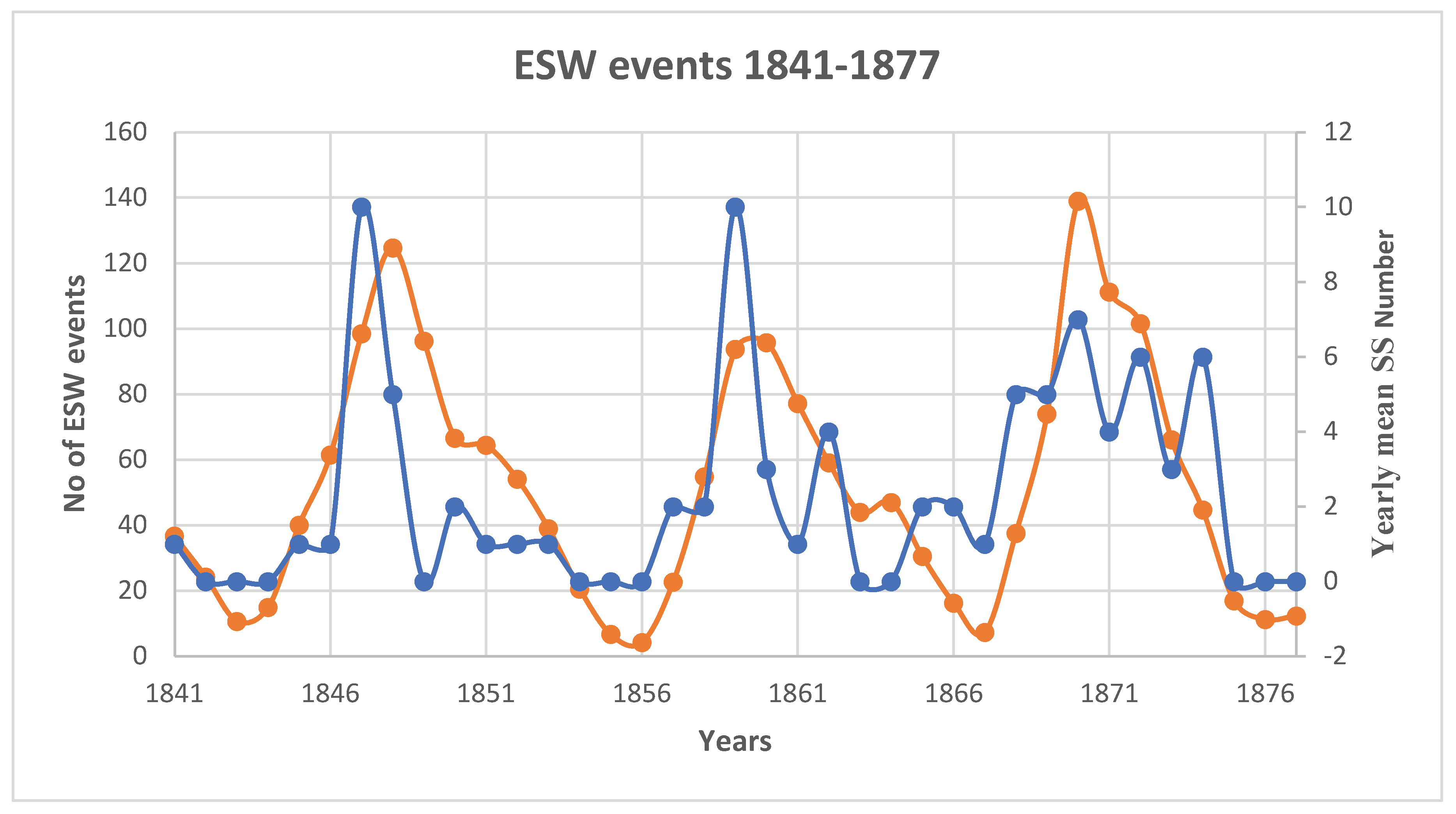
Total number of ESW events ( sum of the number of extreme and super intense storms for the year) for each year between 1841-1877 is plotted in Figure 13 along with international classic sunspot numbers. Characteristic sunspot cycle changes can be seen from this Fig which will be discussed in detail in the next section.
Figure 13.
(a) Daily mean values of H observed in Trivandrum and Singapore calculated by Broun ( 1861) during August-September 1845 (b) Daily mean values of Helsinki Ak and international sunspot number (R) during August-September 1845 ( adopted from Eapen, 2009).
Figure 13.
(a) Daily mean values of H observed in Trivandrum and Singapore calculated by Broun ( 1861) during August-September 1845 (b) Daily mean values of Helsinki Ak and international sunspot number (R) during August-September 1845 ( adopted from Eapen, 2009).
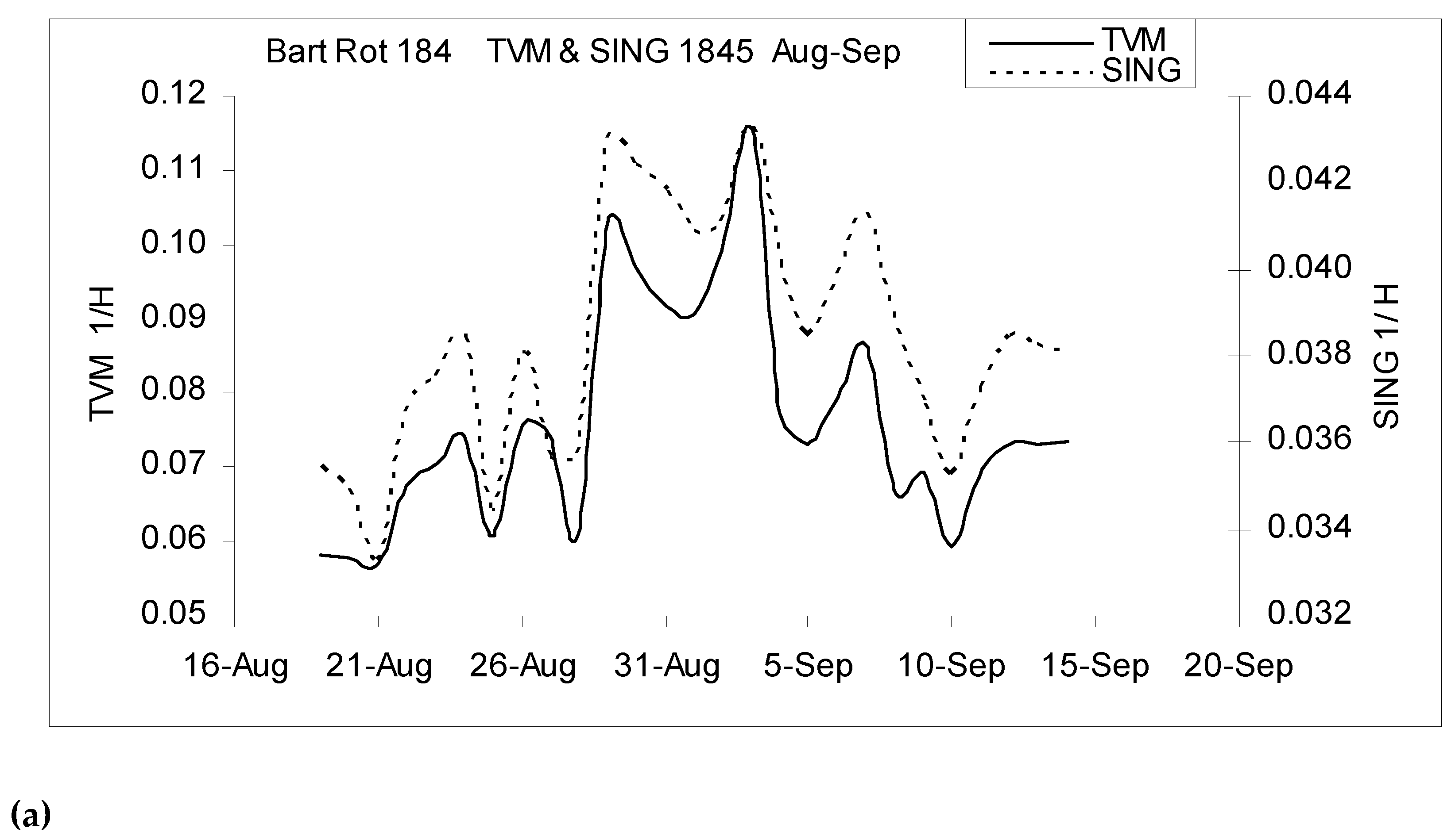
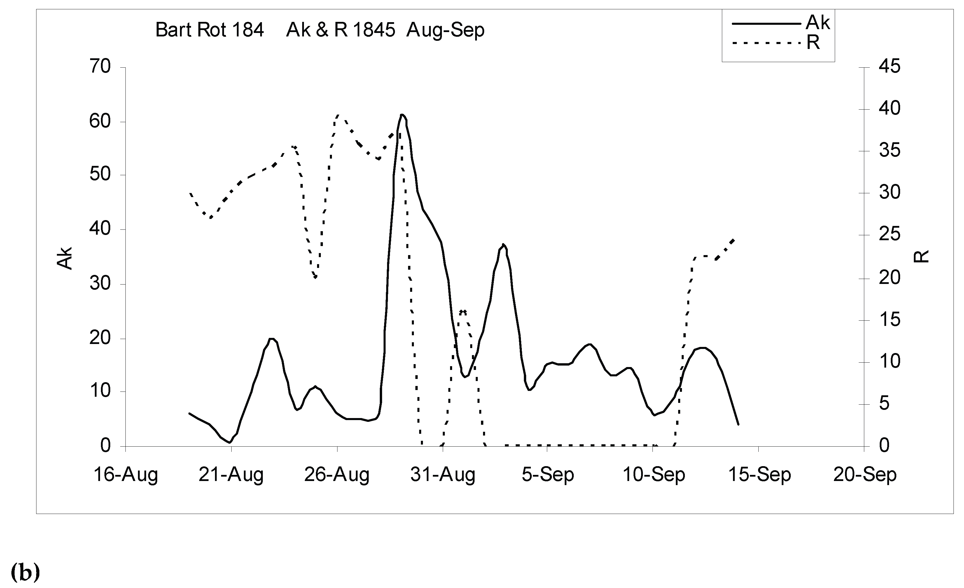
Figure 13.
Annual number of extreme space weather ( ESW) events plotted along with yearly mean international sunspot number for the years 1841-1877.
Figure 13.
Annual number of extreme space weather ( ESW) events plotted along with yearly mean international sunspot number for the years 1841-1877.
8. Discussion
Geomagnetic observations made at British colonial observatories in low/equatorial latitudes during the 19th century under the directions of Royal society of London forms an important resource for inferring the characteristics of extreme space weather events during this period. We aim to identify extreme space weather events during the years 1841-1877 using hitherto unexplored geomagnetic observations in Trivandrum, Madras, Singapore and Bombay located in m either low or equatorial magnetic latitudes.
Only part of Bombay and Trivandrum magnetic observations during the 19th century are studied so far and reported. Ours is a detailed study making use of most of the available archival/published observations related to the above observatories. One of our key objectives is to estimate the intensity of major geomagnetic storms during the period of study and also determine its relation with modern Dst index. During 1841-1855 we have used low latitude observations from Singapore and Madras . We have used of Trivandrum observations which is situated close to the dip equator during the years 1855-1877. Our work will add more light on the results of previous works based on mid latitude observations
The intensity of geomagnetic storms observed in Madras, Singapore and Trivandrum is first determined by scaling storm time changes in daily mean H values in these places to Bombay hourly H observatios . Such an attempt is done by us earlier using limited data series ( Eapen and Girish, 2010; Eapen and Girish, 2012) . Subsequently we have scaled storm time changes in daily mean H values in Trivandrum ( 1841-1845) Madras ( 1846-1855) and Singapore ( 1841-45) to modern Dst values by defining a new index called Tvm Dst.
We have taken care to minimise errors when we determine the intensity of geomagnetic storms in the Dst scale. Reliable Dst estimates are available in literature only for few outstanding storms ( Hayakawa et al., 2022; Hayakawa et al., 2023) . during the period of our investigation in the 19th century. Tvm Dst values are estimated by us using Carrington storm Dst value as a reference. For the Feb 4, 1872 storm, Tvm Dst estimated using Adies Bifilar 1 observations in Trivandrum obslueervatory is found to be 671 nT. If we use normalised Adies Bifilar 2 observations in Trivandrum for the same storm ( see Table ) Tvm Dst value increases to 767 nT. Both these values are found to be less than the Dst value estimated for this outstanding storm (852 nT ) from low latitude observations ( Hayakawa et al., 2023).Further we have normalised the Adies Bifilar observations in Trivandrum during the years 1873-1877 as explained in Sec . and Appendix. So it appears that we have not over estimated the values of Tvm Dst in the present study.
From Figure 13 we can find that the sunspot cycle variations in the annual number of extreme space weather events (NSW) during the years 1841-1877 suggest several interesting features. The period of our study covers the solar cycles 9-11. The most prominent peak in NSW occurs during the epoch of sunspot maxima in these sunspot cycles. During sunspot cycle 9 the maximum or prominent peak in Nsw occurs during the years 1847 and 1859 in the solar cycles 9 and 10 repectively. These years falls one year prior to the sunspot maximum years. It is interesting to find that occurrences of super/extreme intense storms of 1946 March in sunspot cycle 18 ( Hayakawa et al., 2020), 1989 March in sunspot cycle 22 ( Tsurutani et al., 2024) and 2024 May in current 25th sunspot cycle ( Tula si Ram et al., 2024) happens during the late ascending or sunspot maximum epoch.
Let us consider the peaks in Nsw which occurred during the post sunspot maximum or declining phase of these sunspot cycles. Let us consider the peaks in Nsw which occurred during the years 1851 in sunspot cycle 9, during the year 1862 in sunspot and during the year 1872 in sunspot cycle 11. The double peak structure in geomagnetic storm activity during a sunspot cycle is reported in literature (Gonzalez et al., 1990) A distinct peak in geomagnetic activity is found to occur during solar polar magnetic reversal ( SPR) periods and this feature is used to infer the epoch of SPR during every sunspot cycle back to early 18th century ( Haritha et al. 2018; Haritha, 2023). From these cited studies we can find that the years 1851, 1862 and 1872 fall during the epoch of solar polar magnetic reversal. A recent example is the distinct peak in geomagnetic activity during the year 2003 in sunspot cycle 23 which coincides with SPR during that cycle . In Figure 14 we have plotted annual mean values of geomagnetic aa indices during sunspot cycles 11 and 23 where the distinct peaks during the solar polar reversal years can be clearly seen. These results suggest that the pattern of double peak structure of intense geomagnetic storm activity during a sunspot cycle can be used to predict occurrences of super intense storms in future sunspot cycles.
Sunspot cycle 11 is found to be associated with outstanding space weather activity. The number of ESW events ( 37) inferred to have occurred during this cycle from the present study is possibly a maxima during the past 185 years. For comparison during sunspot cycle 19 ( most active cycle in recent times) only 23 ESW events are recorded ( see Figure 15 ). Sunspot cycle 10 where Carrington storm occurred is also a cycle with severe space weather activity with 25 ESW events. preceded by solar cycle 9 with 21 ESW events.
Limitations in the Dst index to define the intensity of extreme geomagnetic storms and allied space weather phenomena is pointed in several studies ( Borovsky and Shprits, 2017; Blake et al., 2021; Manu et al., 2024). Both mid latitude and low latitude indices are used to identify extreme space weather events since the 19th century ( Cliver and Svaalgaard, 2004;Vennerstorm et al., 2016) In the space craft era March 13-14: 1989 geomagnetic storm is found to be associated with maximum decrease of Dst index ( 589 nT) . Space weather effects related to this storm is often compared with the same expected during Carrington class super intense storms. Sym H index is suggested as an alternative to Dst index. ( Solovyev et al., 2005) While Dst index is an hourly index, Sym H is a high resolution( making use of 1 minute geomagnetic observations) storm index. During the main phase of March 1989 storm , maximum H decrease ( ΔH=752 nT) is observed in the equatorial station Kodaikanal in Indian longitudes. Unfortunately there are data gaps for this extreme storm day in Trivandrum and Mumbai magnetic observatories so that accurate ΔH determination becomes impossible. In Figure 16 we have shown remarkable H decrease in Kodaikanal during the Maerch 14 1989 storm. It is interesting to observe that the maximum decrease in Sym H index for this storm is reported to be 715 nT. This value is comparable to the Kodaikanal ΔH if make corrections for the Sq amplitude for this station. So ΔH observations in dip equator stations in different longitudes will help us to determine true intensity of extreme intense geomagnetic storms
The ratio of the magnitude of minimum Dst of Carrington storm ( 949 nT ) with the magnitude minimum Dst of March 1989 storm ( 589 nT) can be found to be 1,6. This implies that :
Sym H ( Carrington Storm) = 1.6 X Sym H ( March 1989 storm ) = 1152 nT
From the minute ( every 2-5 minutes eye readings ) magnetic declination data of Trivandrum observatory published by Allan Broun ( Broun, 1874 ) during the Carrington storm we have found that the revised storm time change %D during this storm can be inferred to be 47%. Applying this value to the regression relation (8) we can find a new estimate of Dst to this outstanding storm. It yields a Dst value of 1120 nT which is comparable to the estimates given in literature. So the true mean intensity of the Carrington storm is likely to between 1100-1200 nT from these resuts. As a typical solar-terrestrial relation we have plotted storm time changes in cloud cover observed in Trivandrum during the Carrington storms in Figure 17.
9. Summary of Results
- Using daily mean H observations in the low/equatorial latitude stations : Trivandrum, Singapore and Madras we have inferred the intensity of geomagnetic storms scaled to Dst indices in modern units during the years 1841-1877. Our results are also compared with Bombay and mid latitude geomagnetic observations during these storm periods.
- Extreme space weather (ESW) events are then identified from the list of extreme or super intense geomagnetic storm periods during 1841-1877 .
- Solar cycle evolution of annual number of ESW events during the sunspot cycles 9-11 is found to show a characteristic double peak structure
- Sunspot cycle 11 is found to be a cycle with exceptional space weather activity if consider relevant data for the past 185 years.
- The limitations of the geomagnetic Dst index in deciding the true intensity of geomagnetic storms is also pointed out.
Author Contributions
P.E.Eapen ( Formal analysis, data curation, writing-original draft preparation). T.E.Girish ( Conveptia;ization, methodology, validation, writing-review and editing). G.Gopkumar ( supervision, project administration, resources, writing-review and editing). V.G.Haritha ( methodology, data curation, software, visualization).
Funding
This research received no external funding.
Data Availability Statement
Data will be made available on request.
Acknowledgments
Authors are grateful to National Library of Scotland for providing selected manuscripts of J.A.Broun related to Trivandrum Observatory.
Conflicts of Interest
The authors has no conflict of interest to declare.
Appendix
TRIVANDRUM MAGNETIC OBSERVATORY :DETAILS OF INSTRUMENTS AND OBSERVATIONS ( 1841-1879)
The magnetic observatory in Trivandrum was established during April 1841 .Early geomagnetic observations ( eye readings ) were made once in two hours which later changed to hourly observations during 1855-1864 and finally 5 times a day during 1865-1879. Most of the geomagnetic observations during this period remain unpublished except for the observations of magnetic declination during the years 1852-1869.
John Caldecott period
The instruments and geomagnetic observations during the period 1841-1849 in Trivandrum made under the supervision of John Caldectott ( first director of the observatory) is shown in Table. The organisation of the Trivandrum magnetic observatory during this period is shown in Fig A1
Allan Broun’s period
The instruments and geomagnetic observations during the period 1852-1864 in Trivandrum made under the supervision of J.A Broun ( first director of the observatory) is also shown in Table Further the organisation o Trivandrum magnetic observatory during this period is shown in Fig A2. The details of this plan is given in Addendum
Period after Broun’s retirement (1865-1879)
After retirement of Broun, two scientific assistants ( Kochu Kunju and Cohervay Pillai) trained by him was entrusted to continue geomagnetic observations in Trivandrum . MJ Kochu kunju (KK) was in charge of the magnetic observatory between the years 1865-1874. After the death of him ( KK) Cochervay pillai was in charge of the observatory between the years 1874-1880. The instruments and magnetic observations during the years 1865-1879 is also given in Table.A1 and values of scale coefficients (k) of the bifilar magnetometers is given in Table A2.
Table A1.
Details of magnetic instruments and observations made under different directors of Trivandrum magnetic observatory during the 19th century.
Table A1.
Details of magnetic instruments and observations made under different directors of Trivandrum magnetic observatory during the 19th century.
| Director and period of magnetic observations | Instruments used during this period and nature of observations |
|---|---|
| 1 John Caldecott ( 1841-1849) Bi-hourly eye observations |
i)Bifilar magnetometers for horizontal force measurements ii)Grubbs declinometer for magnetic declination measurements iii)Grubbs vertical force magnetometer iv) Absolute intensity magnetometer for absolute H measurements |
| 2. J.A Broun (1852-1864) Hourly eye observations |
i)Bifilar magnetometers for horizontal force measurements ii)Robinson and Adies balance magnetometers for vertifical force mesurements iii)Grubbs and Adies declinometers iv) Magnetic survey intsruments |
| 3 Assistants of Broun ( 1865-1879) Eye observations made 5 times daily |
i)Bifilar magnetometers for horizontal force measurements ii)Adies balance magnetometer for vertical force measurements iii) Adies and Grubbs unifilar magnetometers for declination measurements |
Table A2.
Details of Bifilar magnetometers used in Trivandrum observatory and estimated unit constants for different years during 1841-1877.
Table A2.
Details of Bifilar magnetometers used in Trivandrum observatory and estimated unit constants for different years during 1841-1877.
| Period of measurement/use |
Type of the Bifilar magnetometer |
Estimated Unit coefficient (k) |
|---|---|---|
| 1841-1847 | 1) Grubbs bifilar with silver wires |
0.000133-0.00014 |
| 1852 | -do- | 0.0001365-0.0001370 |
| 1854 | 2) Grubbs bifilar with platinum wires |
0.0001503-0.0001505 |
| 1854 | 3) Adies Bifilar No1: Platinum wires |
0.0000692-0.00007 |
| 1855 | 4 )Adies Bifilar used in Augustia Obv: Platinum wires |
0.000044-0.0000451 |
| 1869 May to 1872 December | 5) Adies Bifilar No 1 & Adies Bifilar No 2 |
see section in this paper |
| 1873 -1877 | 6) Adies Bifilar No 2 | -do- |
Adies Bifilar Magnetometer
The main components included an eyepiece for observing the magnet located on a pillar a few meters away and a magnet that was hung from above by two cables. This suspended magnet was free to rotate according to the varying horizontal geomagnetic field; the angle at which the magnet came to rest caused the cables holding it to twist. A scale, reflected off a mirror attached to the suspended magnet, was visible through the eyepiece. The eyepiece would show a different marking on the scale depending on the angle of the magnet. This setup enables the calculation of the percentage change in the strength of the horizontal magnetic field relative to the overall horizontal magnetic field at that location.
Equation of Adies bifilar magnetometer in the equilibrium position ( after Broun, 1861a) is mX= (Wab/l) Sin v (A1)
From this we can find
X = (Wab/ml) Sin v (A2) (
m is the moment of the magnet, X is the horizontal component of earths magnetic field at the location, W is the weight suspended , a and b are the distances between bifilar wires from the top and bottom, l is the length of the bifilar wire and v is the angle of twist .
Storm time change in horizontal force from the base line in modern units is given by :
Δ H ( nT ) = HA(nT) k Hdiff (A3)
Here HA is the absolute value of H in the location
Figure A1.
Plan of Trivandrum magnetic observartory established by J.Caldecott during the year 1841 ( after Eapen, 2009). The explanation of symbols in this Plan: D : Position of the Declination Magnetometer. H : Position of the Bifilar Magnetometer. V : Position of the Vertical Component Magnetometer. t : Reading Telescopes. Λ : Table of Osseler’s Anemometer. Ґ : Library and Computing Room.
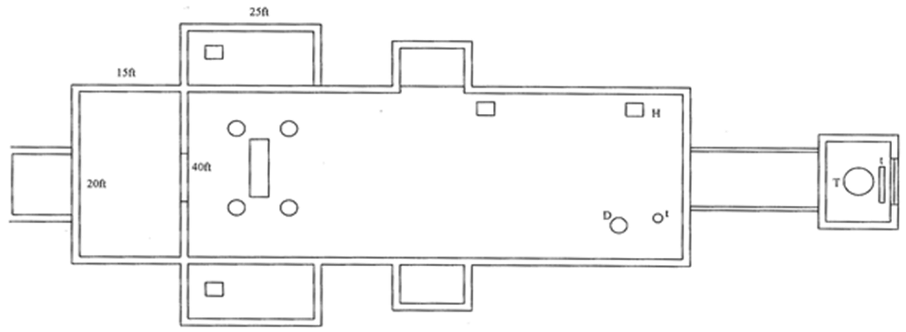
Inference of the intensity of the 1841 storm using Trivandrum H observations
The change in horizontal intensity ( Hd) at Trivandrum during a geomagnetic storm is given by the expression ( Eapen, 2009)
Hd (nT) = (36000/7.8) X Ha X Hd ( sc dev) X k (A4)
Here Ha is the absolute value of H measured in Trivandrum and k is the unit coefficient of the bifilar magnetometer used for the measurement of H variations in this station.
The magnetic observations in 1841 under the supervision of John Caldecott consisted of measurements of magnetic declination, horizontal component (H) and vertical component ( Z) of the geomagnetic field for every two hours in Trivandrum. This is modified to hourly observations since 1852 by John Allan Broun , the second director if Trivandrum observatory.
We have some useful observations of horizontal intensity in Trivandrum during the September 24-25 magnetic storm period as published by British Astronomer Col. Sabine ( Sabine, 1842).
Using Equation (A11) we can calculated the storm intensity for this storm in modern units
From Sabine ( 1842 ) we could find the following data for Trivandrum for this storm:
k= 0.000133
Ha= 7.77 BU
Maximum storm time change in bi-hourly H in Trivandrum is
Hd = 49.3 Sc div
Intensity of 1841 Sep 24-25 storm in Trivandrum from (A4) = 235.14 nT/.
Theory for simultaneous measurement of H with two different bifilars
Let Hd1 and Hd2 are the readings of the bifilar magnetometers 1 and 2 corresponding to change in H during a geomagnetic storm period expressed in scale divisions. Now from equation (x) we can write :
Hd (nT) = Q X Ha X Hd1 (sc div) X k1 = Q X Ha X Hd2 ( sc div) X k2 (A5)
Here Q = 36000/7.8
Ha is the absolute value of H in the station close to the storm period
k1 and k2 are the unit coefficients of bifilar 1 and bifilar 2 respectively.
From (A5) we can find that
Hd1 k1 = Hd2 k2
(Hd1/Hd2) = (k2/k1) =k
Hd1= k X Hd2
Figure A2.
Plan of the Trivandrum magnetic observatory under the supervision of Broun.J.A (after Eapen, 2009).
Figure A2.
Plan of the Trivandrum magnetic observatory under the supervision of Broun.J.A (after Eapen, 2009).
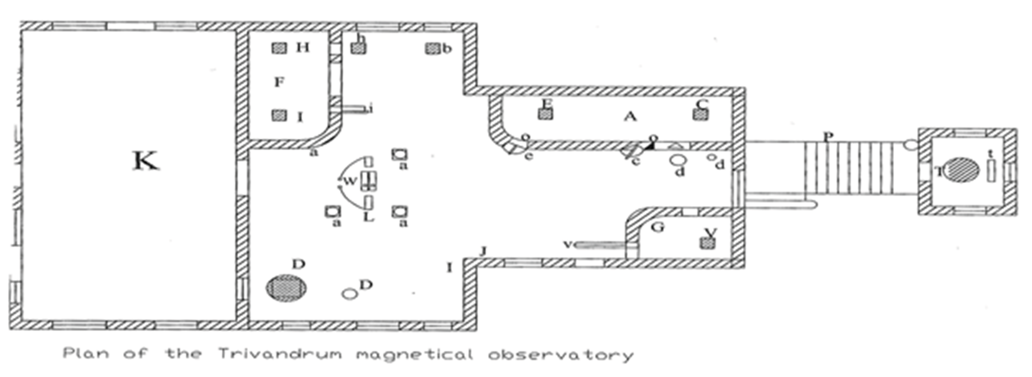
Fig. A2 depicts the Trivandrum magnetic observatory’s layout (Elliot, 1898) during the supervison of Broun in 1850’s. Up until 1853, the declinometer (Dr. Lloyd’s by Mr. Grubb of Dublin) and its reading telescope d’ were located on pillar d. In the little transit house north of the observatory, a transit instrument was positioned on pillar T, slightly out of azimuth, but connected to it via the exposed tunnel P. The transit was so tuned that the declination telescope d’ could serve as a collimator to transit when it was inverted on its Ys. The transit instrument was then used to observe stars in order to establish the azimuth of d’\
The pillars’ locations with Grubb’s bifilar and telescope up until 1853 are displayed at D, D’. Robinson’s magnetometer was located in pillar H until its removal in 1859. The plan shows the various modifications made to the observatory in 1853. The bifilar and its telescope were put on the pillars constructed at b and h, while Grubb’s declinometer and its telescope were moved from the previously designated pillars to those previously occupied by the latter.
In October 1853, room A was constructed inside the observatory. It was completely enclosed above by a ceiling made of well-joined, one-inch-thick teak planks, covered in plaster like a terraced roof, and had only one opening at Δ, which was closed by a double door that opened inward and outward, as well as at o o small apertures that were sealed by the ivory or glass scales and the object glass of the telescopes. At the end of 1853, two additional instruments built in accordance with Mr. Broun’s directions by Mr. Adie of London occupied the pillars C and E in this closed room. The telescopes for these instruments were positioned on the pillars e and e, forming a portion of the well-founded wall.For a new balance magnetometer made for Mr. Broun, also by Mr. Adie of London, a comparable closed room was constructed at G; its telescopes are displayed at V and v.
A third closed room was constructed at F in 1859, with pillars H and I holding various instruments at different times.Adie’s second bifilar, which had previously been used at the Agustia Malley Observatory, was installed on pillar H in 1859, while the balance from the same observatory was installed on pillar I. These instruments were identical in construction to those on pillars E and V (Figure 2.4). These two devices’ telescopes were housed in pillars h and i. In order to conduct additional observations at the Agustia Observatory, these instruments
were taken out in 1864 and reinstalled in 1865.
During the period 1864-65
Dr. Lamont’s small instruments, which were acquired from his Munich observatory earlier , occupied the pillars. H was used for the horizontal force instrument, while I was used for the induction apparatus. The former was used for variations of horizontal force, while the latter was used for vertical force.
References
- Airy, George Biddell. First analysis of one hundred and seventy-seven magnetic storms, registered by the magnetic instruments in the Royal Observatory, Greenwich, from 1841 to 1857. Phil. Trans. R. Soc. 1863, 153, 617–648. [Google Scholar] [CrossRef]
- Blake, S. P.; Pulkkinen, A.; Schuck, P. W.; Glocer, A.; Oliveira, D. M.; Welling, D.; et al. Recreating the horizontal magnetic field at Colaba during the Carrington event with geospace simulations. Space Weather 2021, 19, e2020SW002585. [Google Scholar] [CrossRef]
- Blake, S. P.; Pulkkinen, A.; Schuck, P. W.; Nevanlinna, H.; Reale, O.; Veenadhari, B.; et al. Magnetic Field Measurements from Rome during the August-September 1859 Storms. Journal of GeophysicalResearch: Space Physics 2020, 125, e2019JA027336. [Google Scholar] [CrossRef]
- Borovsky, J. E.; Shprits, Y. Y. Is the Dst index sufficient to define all geospace storms? Journal of Geophysical Research: Space Physics. 2017, 122(11), 543–11,547. [Google Scholar] [CrossRef]
- Broun, JA. On the Horizontal Force of the Earth’s Magnetism. Trans/Roy.Soc.Edin 1861, 22(3), 511–565. [Google Scholar] [CrossRef]
- Broun, J.A. The Bifilar magnetometer: its Errors and Corrections. Proc Roy.Soc.Edin 1862, 4, 406–407. [Google Scholar] [CrossRef]
- Broun, J.A. Observations of Magnetic Declinations made at Trivandrum and Agustia Malley in the observatories of His Highness The Maharajah of Travancore, G.C.S.I in the years 1852-1869. In Trivandrum Magnetical Observations Volume I; Henry S King & Co: London, 1874. [Google Scholar]
- Broun, J.A. On the influence of height in the atmosphere on the diurnal variation of the earth’s magnetic force. Proc. R. Soc 1877, 25(171-178), 566–569. [Google Scholar] [CrossRef]
- Chambers, C. Magnetical and Meteorological Observations made at the Government Observatory; Govt of Bombay Publication: Bombay, 1852. [Google Scholar]
- Chapman, S.; Gupta, J.C. Solar and Lunar daily variations of declination at Trivandrum 1853-1869. Pageoph 1971, 87, 93–101. [Google Scholar] [CrossRef]
- Cliver, E.W.; Svalgaard, L. The 1859 Solar–Terrestrial Disturbance And the Current Limits of Extreme Space Weather Activity. Sol Phys 2004, 224, 407–422. [Google Scholar] [CrossRef]
- Cliver, E.W.; Schrijver, C.J.; Shibata, K.; et al. Extreme solar events (2002). Living Rev Sol Phys 19, 2. [CrossRef]
- Eliot, C.M. Magnetical observations made at the Hon. East India company magnetic observatory at Singapore in the years 1841-45; American mission and Male Asylum publication: Madras, 1850. [Google Scholar]
- Elliot, C.M. Magnetic survey of the Eastern Archipelago. Phil. Trans. R. Soc. 1851, 31, 287–331. [Google Scholar] [CrossRef]
- Fergusson, F. T. Magnetical and Meteorological Observations Made at the Government Observatory:Bombay; Bombay Education Society’s Press: Bombay, 1860. [Google Scholar]
- Ganushkina, N.; Jaynes, A.; Liemohn, M. Space Weather Effects Produced by the Ring Current Particles. Space Sci Rev 2017, 212, 1315–1344. [Google Scholar] [CrossRef]
- Gautam S, Sarup Khadka Saurav, Binod Adhikarib, Santosh Sapkota,Parashu Ram Poudel, Roshan Kumar Mishra, and Chhabi Kumar Shrestham. Variation of the H Component of Geomagnetic Field:Relationship to the Ring and Field Aligned Currents. Kinematics and Physics of Celestial Bodies 2023, 39, 10–23. [CrossRef]
- Gawali, P. B.; Doiphode, M. G.; Nimje, R. N. : Colaba–Alibag magnetic observatory and Nanabhoy Moos: the influence of one over the other (2015). Hist. Geo Space. Sci. 6, 107–131. [CrossRef]
- Gonzalez, W.D.; Gonzalez, A.L.C.; Tsurutani, B.T. Dual-peak solar cycle distribution of intense geomagnetic storms. Planet. Space Sci. 1990, 38, 181–187. [Google Scholar] [CrossRef]
- Haritha, V G; Eapen, P E; Gopkumar, G; Girish, T E. On the Characteristics of Geomagnetic Storms Observed During the Past 415 Years. In Long-Term Datasets for the Understanding of Solar and Stellar Magnetic Cycles Proceedings IAU Symposium No. 340; Banerjee, D., Jiang, J., Kusano, K., Solanki, S., Eds.; 2018; pp. 153–154. [Google Scholar]
- Haritha, V.G. Studies on the Association of Large scale magnetic fields with some Solar-Terrestrial Phenomena. PhD Thesis, University of Kerala, Trivandrum, India, 2023. [Google Scholar]
- Hayakawa Hisashi, Heikki Nevanlinna, Séan P. Blake, Yusuke Ebihara, Ankush T. Bhaskar, and Yoshizumi Miyoshi. Temporal Variations of the Three Geomagnetic Field Components at Colaba Observatory around the Carrington Storm in 1859. Ap 2022, J, 928, 32.
- Hayakawa, Hisashi; Ebihara, Yusuke; Pevtsov, Alexei; Bhaskar, Ankush; Karachik, Nina; Oliveira, Denny M. Intensity and time series of extreme solar-terrestrial storm in 1946 March. MNRAS 2020, 497, 5507–5517. [Google Scholar] [CrossRef]
- Hejda, P.; Valach, F.; Revallo, M. Historical geomagnetic observations from Prague observatory (since 1839) and their contribution to geomagnetic research. Hist. Geo Space. Sci. 2023, 14, 51–60. [Google Scholar] [CrossRef]
- Hisashi, Hayakawa; et al. The Extreme Space Weather Event of 1872 February: Sunspots, Magnetic Disturbance, and Auroral Displays. ApJ 2023, 959, 23. [Google Scholar] [CrossRef]
- Indian magnetic data (2005) Annual Data books of IIG: 1974-1996 ( Geomagnetic data of Indian stations) EGRL; Tirulveli.
- Jacob, W.S. Magnetical observations made at the Hon. East India Company observatory at Madras in the years 1851-1855; Lawrence Asylum Press: Madras, 1884. [Google Scholar]
- James, M.E; Rastogi, R.G; Winch, D.E. Magnetic disturbance effect on geomagnetic field at low latitudes. Ind.J.Radio Space Phys. 2004, 33, 88–94. [Google Scholar]
- Jayakrishnan, R, C.K. Fazil, L. Rahul Dev, and A. Ajesh. Unravelling the detection of Carrington storm of 1859 from the historical magnetic declination observations of Trivandrum observatory. Adv Space. Res. 2025, 76, 3670–3680. [CrossRef]
- Jones, H.S. Sunspot and Geomagnetic storm data; His Majesties Stationary Office: London, 1955. [Google Scholar]
- Kotadia, K.M. Equatorial sporadic E ionization and electrojet effect of geomagnetic disturbances. Proc. Indian Acad. Sci. 1964, 60, 352–367. [Google Scholar] [CrossRef]
- Kumar, S.; Veenadhari, B.; Tulasi Ram, S.; Selvakumaran, R.; Mukherjee, S.; Singh, R.; Kadam, B. D. Estimation of interplanetary electric field conditions for historical geomagnetic storms. J. Geophys. Res. Space Physics 2015, 120, 7307–7317. [Google Scholar] [CrossRef]
- Lakhina, G.S; Tsurutani, Bruce T. Chapter 7 - Supergeomagnetic Storms: Past, Present, and Future. In Extreme Events in Geospace; Buzulukova, Natalia, Ed.; Elsevier, 2018; pp. pp 157–185. [Google Scholar] [CrossRef]
- Mandea, M.; Chambodut, A. Geomagnetic Field Processes and Their Implications for Space Weather. Surv Geophys 2020, 41, 1611–1627. [Google Scholar] [CrossRef]
- Manu, V.; Balan, N.; Ebihara, Y.; et al. A fresh look at the intensity and impulsive strength of geomagnetic storms. Geosci. Lett. 2024, 11, 22. [Google Scholar] [CrossRef]
- Maunder, E.W. Magnetic Disturbances as recorded at the Royal Observatory, Greenwich, and their Association with Sun-spots. Second Paper, MNRAS 1905, 65(6), 538–559. [Google Scholar] [CrossRef]
- Moos, N.A.F. Magnetic Observations made at the Govt Observatory, Bombay for the years 1846-1905:Part I-Magnetic Data and Instruments; Govt Central Press: Bombay, 1910. [Google Scholar]
- Moos, NAF. Magnetic observations made at the Govt observatory Bombay 1846-1905- Part II: The Observations and its Discussion; Govt of Bombay publication: Bombay, 1910. [Google Scholar]
- Nevanlinna, H. Results of the Helsinki magnetic observatory 1844–1912. Ann. Geophys. 2004, 22, 1691–1704. [Google Scholar] [CrossRef]
- NLS. Comparison of daily means of Bifilar-1 and Bifilar-2 with Tables of daily means of horizontal forces: 1855-1864. In Manuscripts of John Allan Broun: Inventory No Acc 10064-No 75; National Library of Scotland, UK, 2007a. [Google Scholar]
- NLS. Magnetic observations made at the Trivandrum Observatory: 1865-1879. In Manuscripts of John Allan Broun: Inventory No Acc 10064-No 75; National Library of Scotland, UK, 2007b. [Google Scholar]
- Panda, S.K.; Gedam, S.S.; Rajaram, G.; et al. A multi-technique study of the 29–31 October 2003 geomagnetic storm effect on low latitude ionosphere over Indian region with magnetometer, ionosonde, and GPS observations. Astrophys Space Sci 2014, 354, 267–274. [Google Scholar] [CrossRef]
- Ptitsyna, N.G; Tyasto, M. I.; Khrapov, B. A. Great Geomagnetic Storms in 1841–1870 according to the Data from the Network of Russian Geomagnetic Observatories. Geomag. Aeron. 2012, 52, 613–623. [Google Scholar] [CrossRef]
- Rao, M.P. Auroal Observations in India. Mausam 1964, 15, 639–644. [Google Scholar] [CrossRef]
- Rastogi, R.G. Geomagnetic storm effects at low latitudes. Annales Geophysicae 1999, 17, 438–441. [Google Scholar] [CrossRef]
- Royal Society. Report of the committee of Physics including Meteorology, on the objects of scientific enquiry in those sciences; Richard and Taylor Publication: London, 1840; pp. pp 1–52. [Google Scholar]
- Sabibe. E (1842) Observations made at the Magnetic Observatory at Toronto, during a remarkable Magnetic Disturbance on the 25th and 26th of September, 1841; with Postscripts, containing the Observations of the same Disturbance made at the Magnetic Observatories of Trevandrum, St. Helena, and the Cape of Good Hope. In Rep 11th Meeting of Brit Assn for the Adv Sci; pp. pp 340–356.
- Solovyev, SI; Boroyev, R.N.; Moiseyev, A.V. On the relation between the Sym-H and Dst- indices during the development of magnetic storm, in: Physics of Auroral Phenomena. Proc. XXVIII Annual Seminar, Apatity, 2005; pp. 48–51. [Google Scholar]
- Stamper, R.; Lockwood, M.; Wild, M. N.; Clark, T. D. G. Solar causes of the long-term increase in geomagnetic activity. J. Geophys. Res. 1999, 104(A12), 28325–28342. [Google Scholar] [CrossRef]
- Taylor, T.G. Observations of the Magnetic Dip and Intensity at Madras in 1837. Jl.Asiatic Soc. Bengal, in 1837 1837, 6(issue 65), 374–377. [Google Scholar]
- Taylor, T.G.; Caldecott, J. Observations on the direction and intensity of the terrestrial magnetic force in Southern India. Madras J. Lit. Sci. 1839, 9, 221–272. [Google Scholar]
- Taylor, T.G; Worster, W.K.; Jacob, W.S. Magnetic Observations made at the East India Company’s magnetic observatory at Madras in the years 1846-1850; American Mission Press: Madras, 1854. [Google Scholar]
- Tsurutani, B. T.; Sen, A.; Hajra, R.; Lakhina, G. S.; Horne, R. B.; Hada, T. Review of the August 1972 and March 1989 (Allen) space weather events: Can we learn anything new from them? of Geophysical Research: Space Physics 2024, 129, e2024JA032622. [Google Scholar] [CrossRef]
- Tulasi Ram, S.; Veenadhari, B.; Dimri, A.P.; Bulusu, J.; Bagiya, M.; Gurubaran, S.; et al. Super-intense geomagnetic storm on 10–11 May 2024: Possible mechanisms and impacts. Space Weather 2024, 22, e2024SW004126. [Google Scholar] [CrossRef]
- Tulasi Ram, S.; Veenadhari, B.; Dimri, A.P.; Bulusu, J.; Bagiya, M.; Gurubaran, S.; et al. Super-intense geomagnetic storm on 10–11 May 2024: Possible mechanisms and impacts. Space Weather 2024, 22, e2024SW004126. [Google Scholar] [CrossRef] [PubMed]
- Veenadhari, B; Alex, S. Space weather effects on low latitude geomagnetic field and ionospheric plasma response. Proc. ILWS Workshop 2006, Goa, India, 2006. [Google Scholar]
- Vennerstrom, S.; Lefevre, L.; Dumbović, M.; et al. Extreme Geomagnetic Storms – 1868 – 2010. Sol Phys 2016, 291, 1447–1481. [Google Scholar] [CrossRef]
- Villaverde, A.C, Pablo Muñoz and Consuelo Cid. Classifying and bounding geomagnetic storms based on the SYM-H and ASY-H indices. Nat. Haz 2024, 120, 1141–1162. [CrossRef]
Figure 1.
Daily mean H of Madras for the month of February 1852 expressed as fraction of absolute horizontal intensity in British Units. The decrease on Feb 19 is remarkable.
Figure 1.
Daily mean H of Madras for the month of February 1852 expressed as fraction of absolute horizontal intensity in British Units. The decrease on Feb 19 is remarkable.
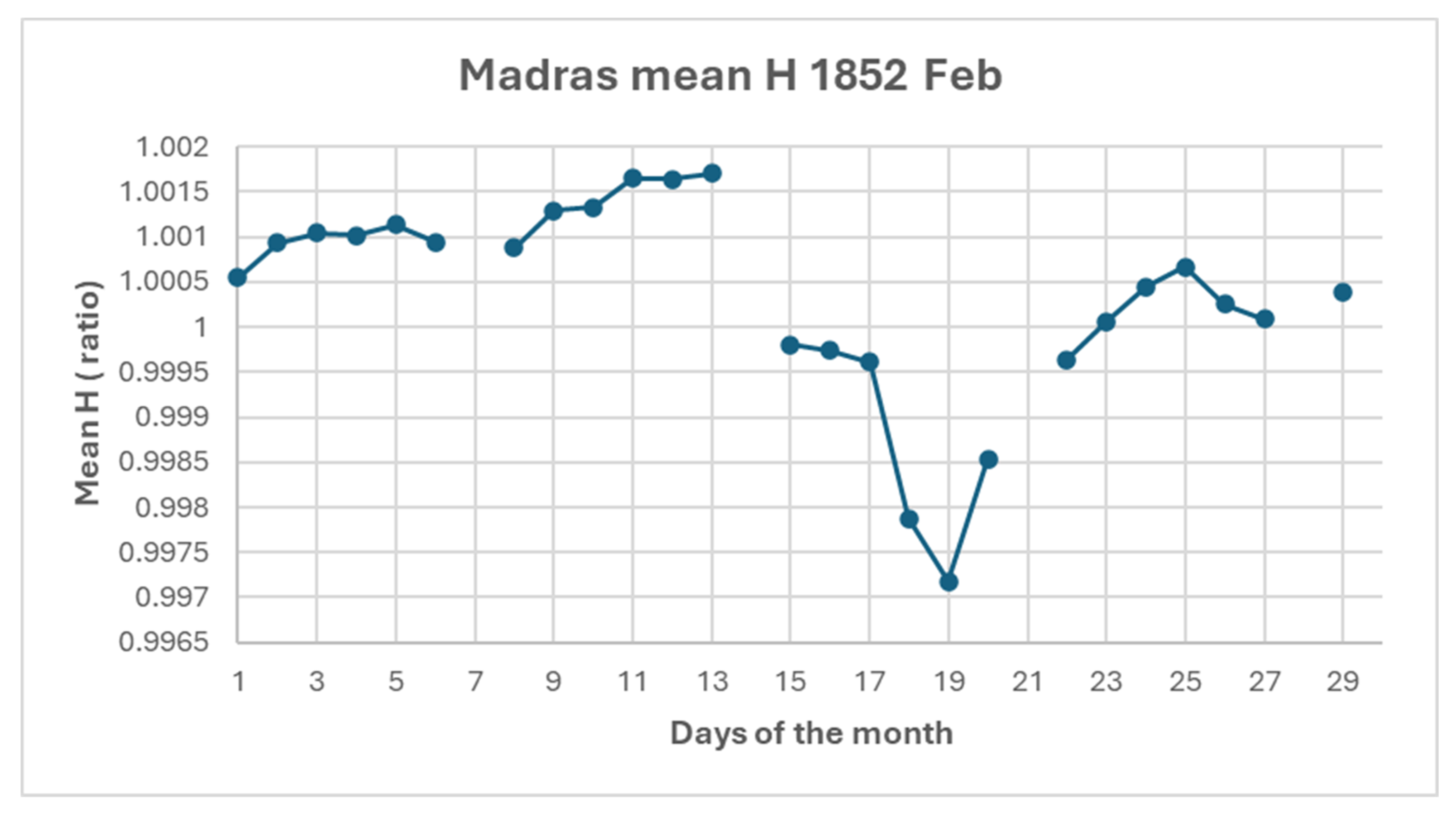
Figure 2.
Regression relation between values of storm time change in daily mean H of Madras ( BU) and Bombay hourly ΔH (nT) for selected geomagnetic storms during 1852-1855.
Figure 2.
Regression relation between values of storm time change in daily mean H of Madras ( BU) and Bombay hourly ΔH (nT) for selected geomagnetic storms during 1852-1855.
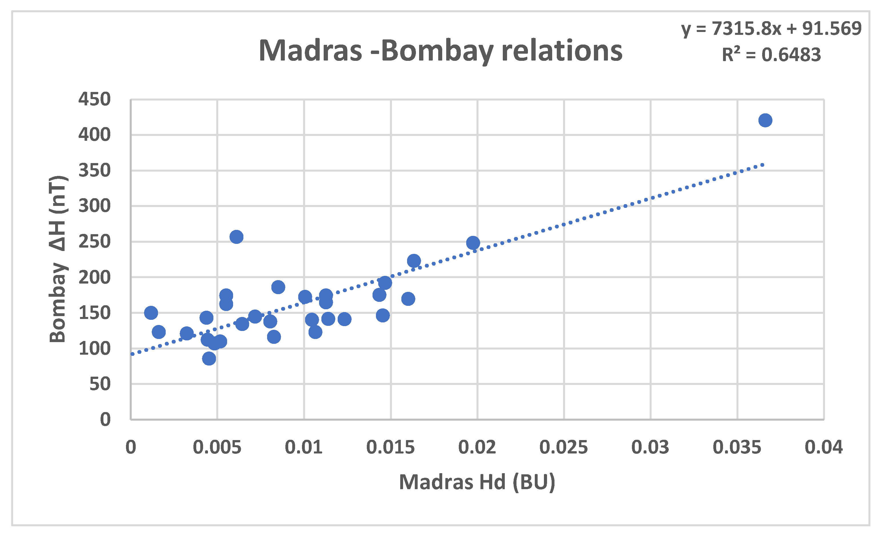
Figure 4.
Regression relation between values of storm time change in daily mean H of Trivandrum (Sc div) and Bombay hourly ΔH (nT) for selected geomagnetic storms during 1855-1863.
Figure 4.
Regression relation between values of storm time change in daily mean H of Trivandrum (Sc div) and Bombay hourly ΔH (nT) for selected geomagnetic storms during 1855-1863.
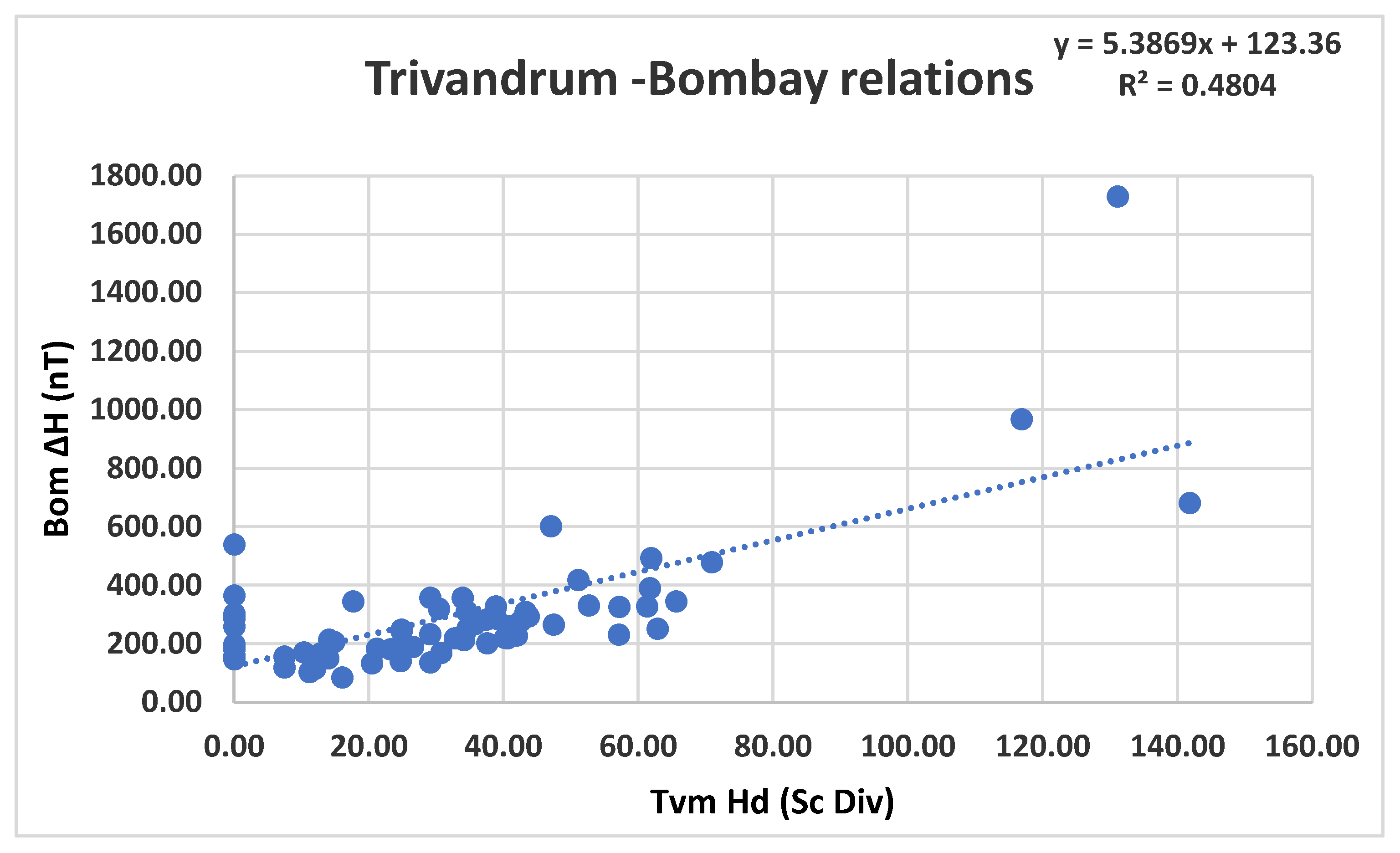
Figure 5.
Variations of Trivandrum magnetic declination (D and % D) and Bombay1/H during the Carrington geomagnetic storm of September 2, 1859.
Figure 5.
Variations of Trivandrum magnetic declination (D and % D) and Bombay1/H during the Carrington geomagnetic storm of September 2, 1859.
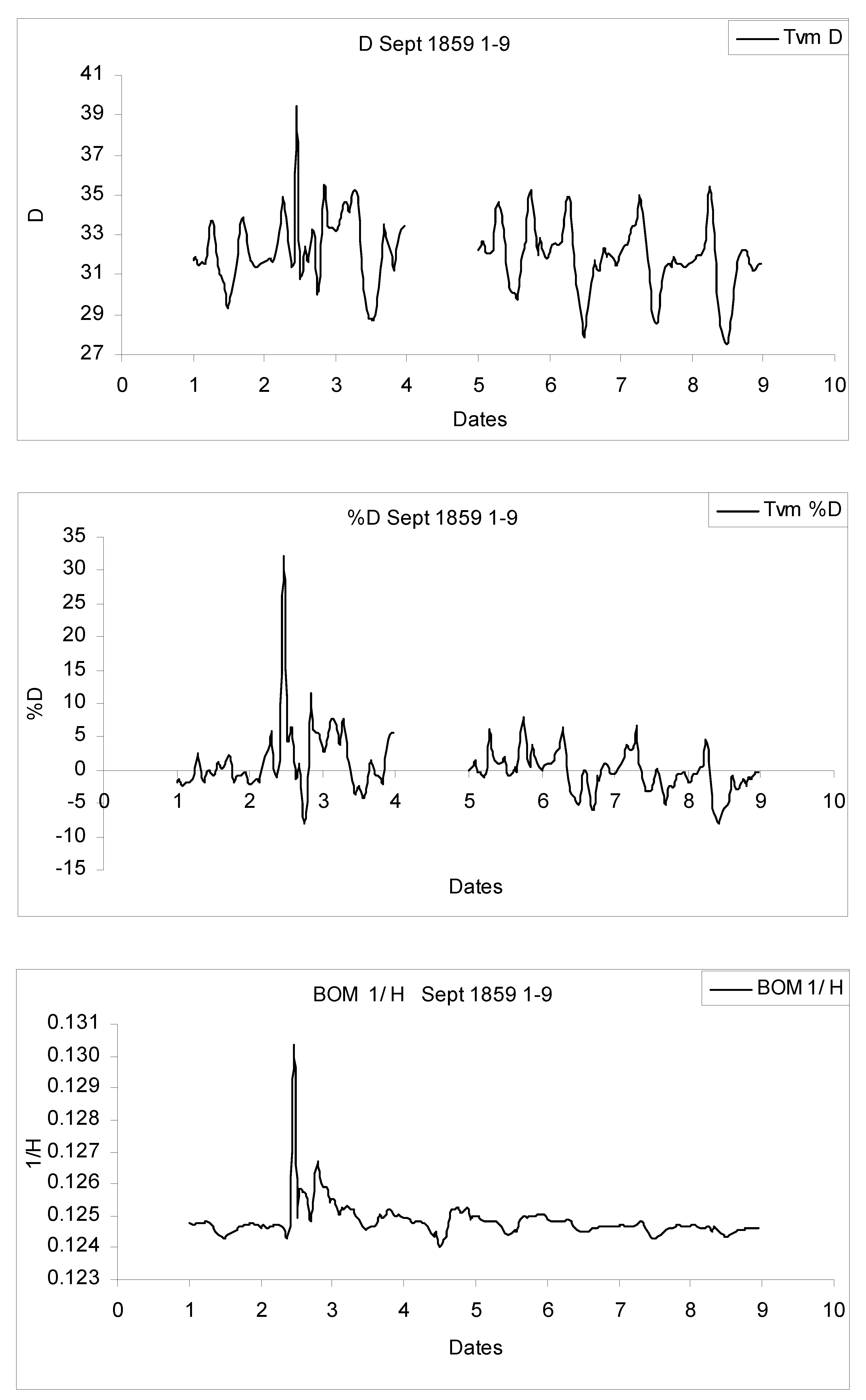
Figure 6.
Variation of D and its storm time differences (%D) observed during the great geomagnetic storm of March 14, 1989 (a) at Trivandrum (b) at Kodaikanal and Annamalai Nagar ( adopted from Eapen, 2009).
Figure 6.
Variation of D and its storm time differences (%D) observed during the great geomagnetic storm of March 14, 1989 (a) at Trivandrum (b) at Kodaikanal and Annamalai Nagar ( adopted from Eapen, 2009).
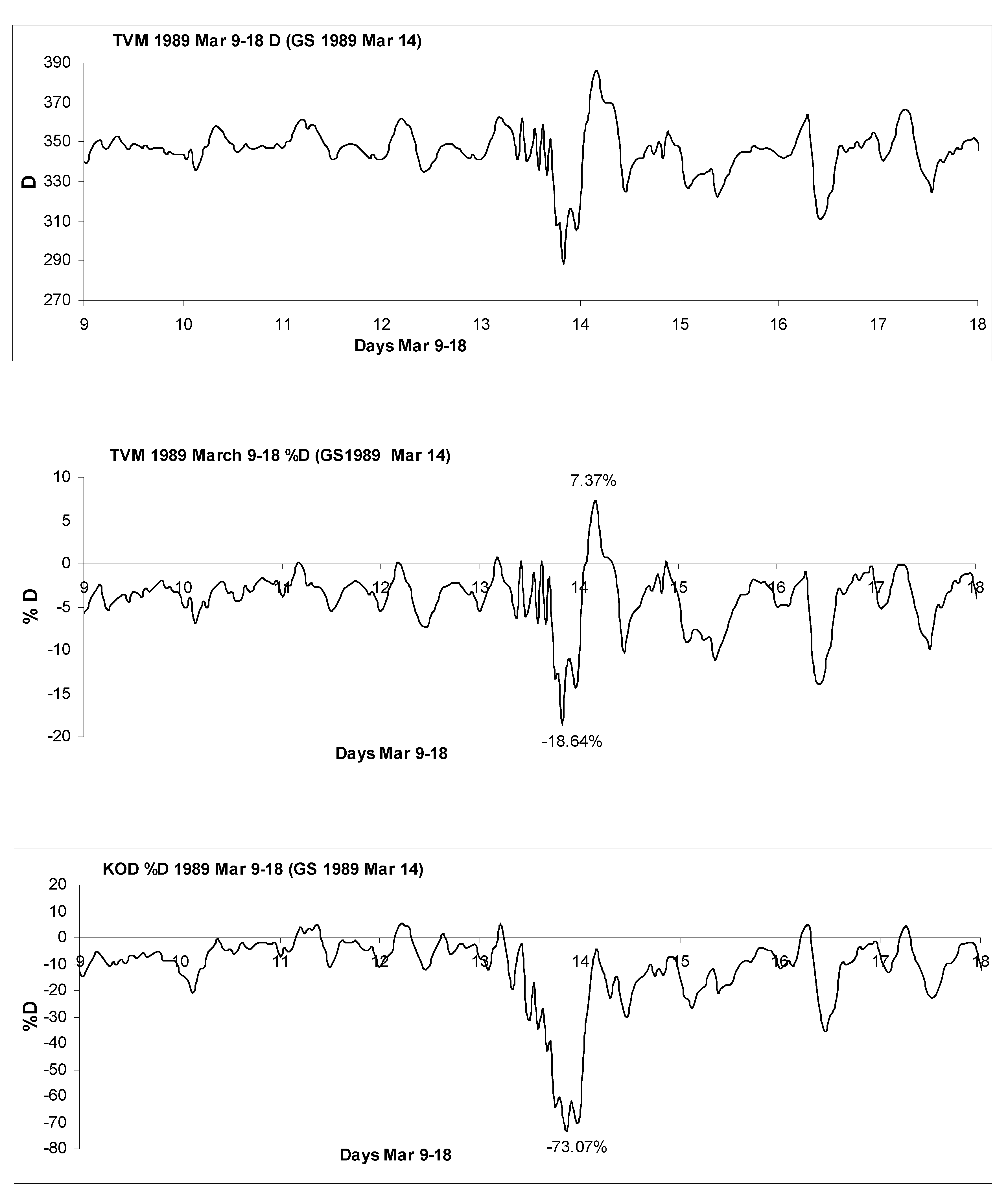
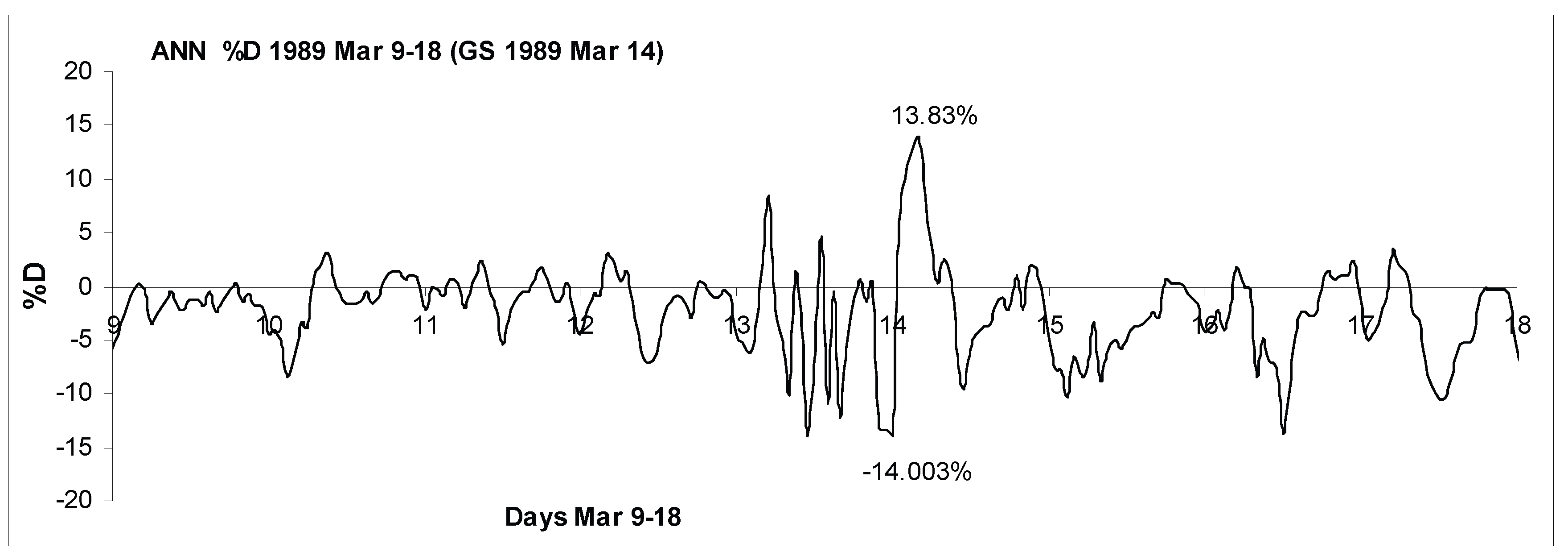
Figure 7.
Linear regression relation between Tvm %D max (maximum storm time hourly change in magnetic declination in Trivandrum ) and magnitude of Dst minimum for selected intense geomagnetic storms during the modern period.
Figure 7.
Linear regression relation between Tvm %D max (maximum storm time hourly change in magnetic declination in Trivandrum ) and magnitude of Dst minimum for selected intense geomagnetic storms during the modern period.
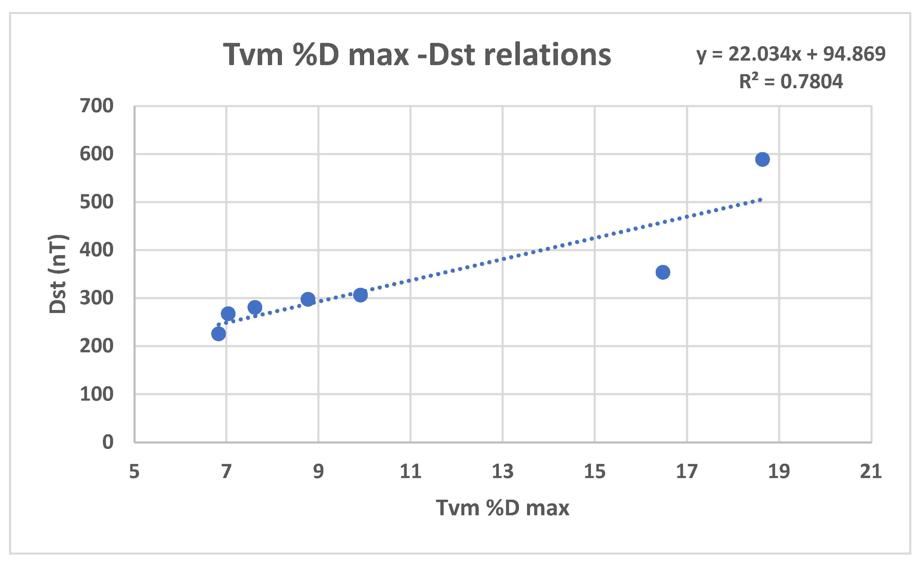
Figure 8.
Regression relation between values of storm time change in daily mean H of Madras (Hd in BU) and Tvm Dst for selected geomagnetic storms during the year 1855.
Figure 8.
Regression relation between values of storm time change in daily mean H of Madras (Hd in BU) and Tvm Dst for selected geomagnetic storms during the year 1855.
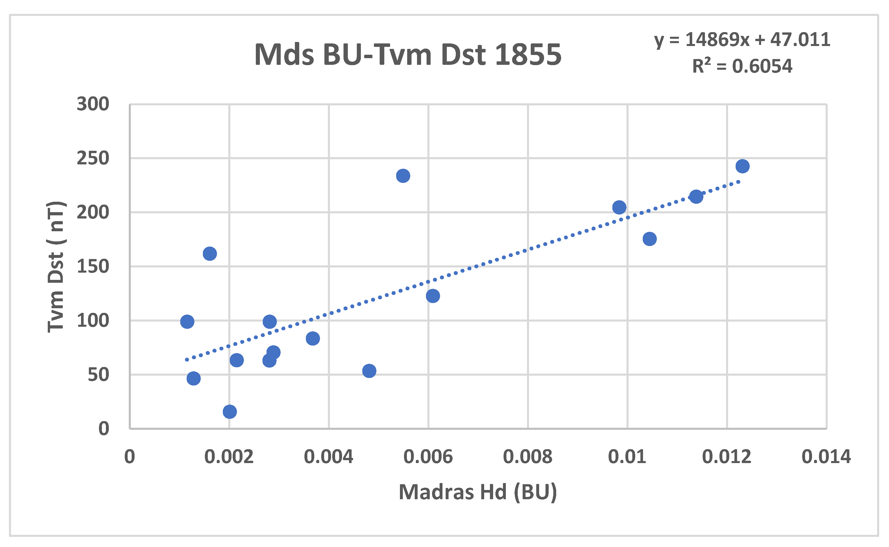
Figure 9.
Linear regression fit between Tvm % ΔH (Devitiation of Storm time value of daily mean H from monthly mean in Trivandrum ) and magnitude of minimum Dst during selected storms in the modern period.
Figure 9.
Linear regression fit between Tvm % ΔH (Devitiation of Storm time value of daily mean H from monthly mean in Trivandrum ) and magnitude of minimum Dst during selected storms in the modern period.
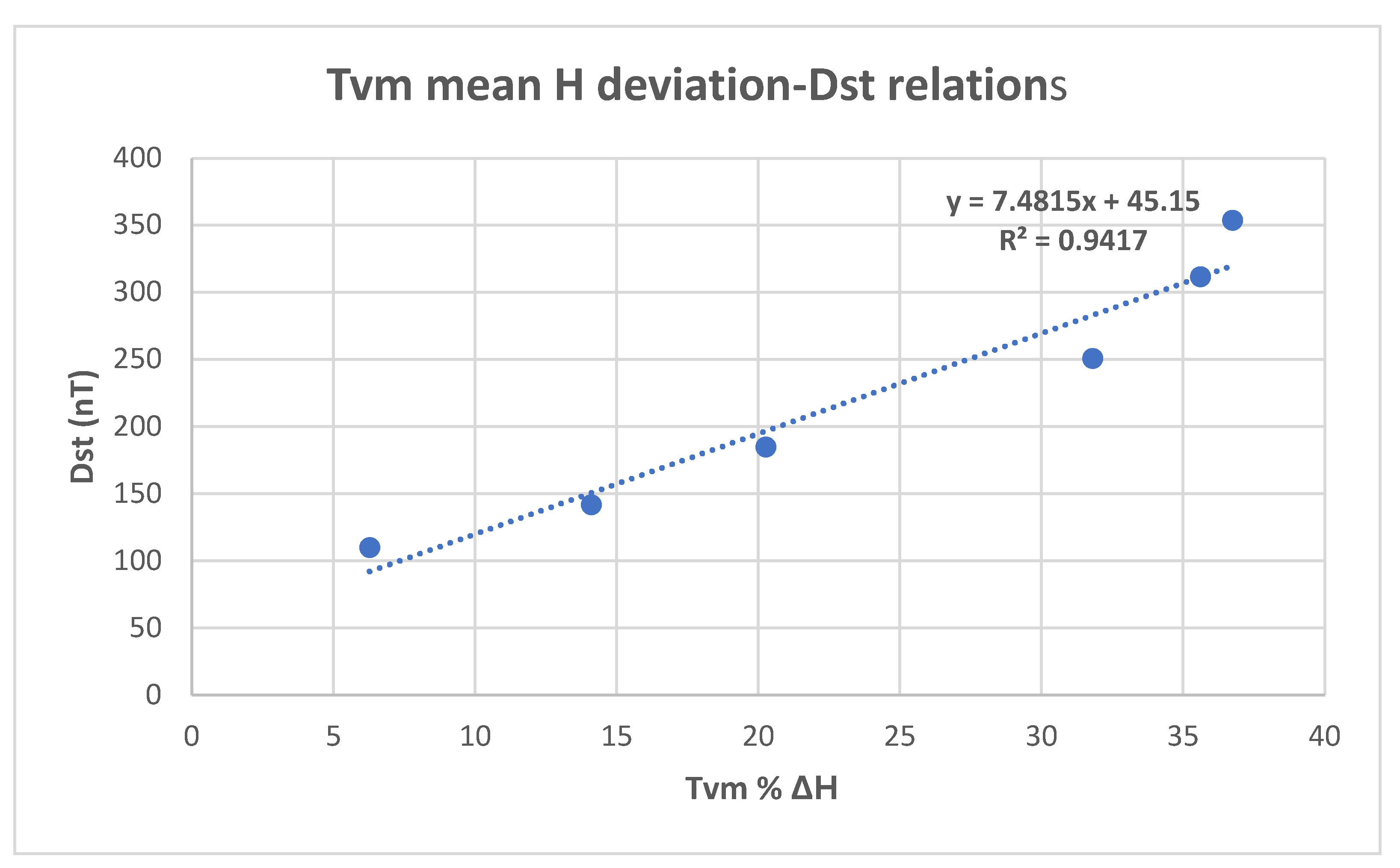
Figure 10.
Linear regression relation between Bombay ΔH ( maximum hourly storm time decrease in Bombay -Alibag observatory) and magnitude of minimum Dst index during selected super intense storms during the years… ( after Lakhina et al. ).
Figure 10.
Linear regression relation between Bombay ΔH ( maximum hourly storm time decrease in Bombay -Alibag observatory) and magnitude of minimum Dst index during selected super intense storms during the years… ( after Lakhina et al. ).
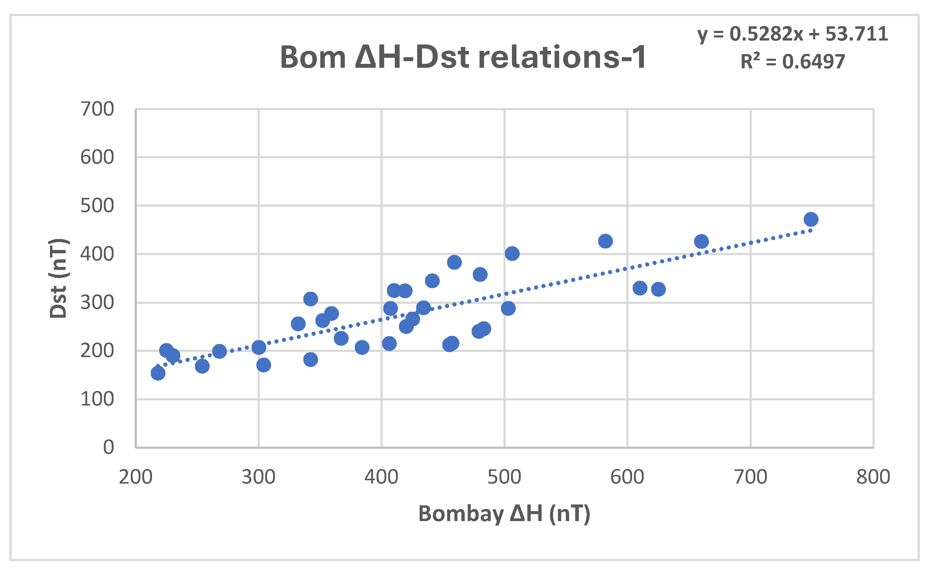
Figure 11.
Linear regression relation between Bombay ΔH ( maximum hourly storm time decrease in Bombay -Alibag observatory) and magnitude of minimum Dst index during selected intense storms during the years… ( after Rawat et al., 2020 ).
Figure 11.
Linear regression relation between Bombay ΔH ( maximum hourly storm time decrease in Bombay -Alibag observatory) and magnitude of minimum Dst index during selected intense storms during the years… ( after Rawat et al., 2020 ).
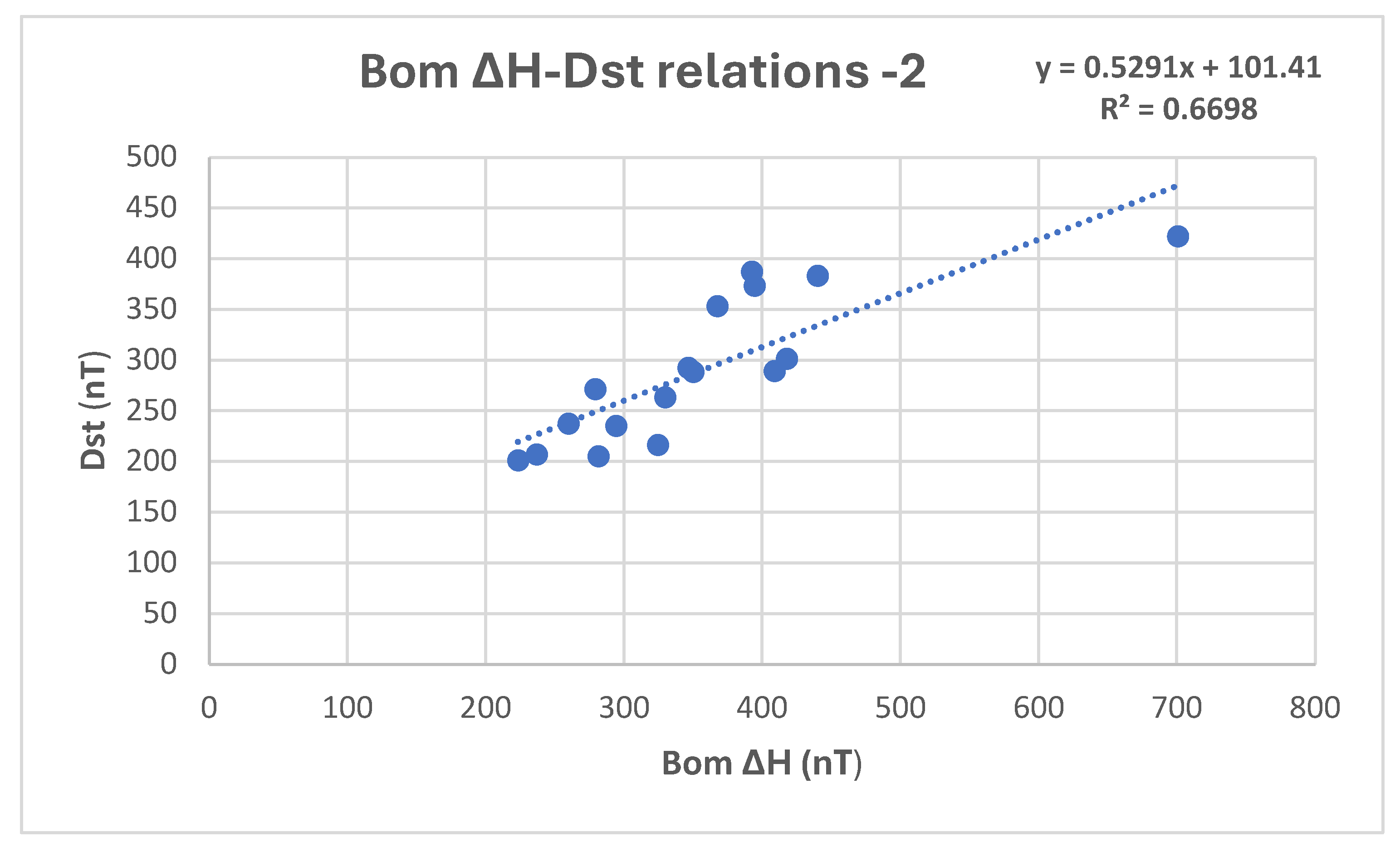
Figure 12.
Regression fit between ΔHE (Maximum storm time decrease in hourly H in equatorial stations ) and magnitude of minimum Dst values for selected modern geomagnetic storms.
Figure 12.
Regression fit between ΔHE (Maximum storm time decrease in hourly H in equatorial stations ) and magnitude of minimum Dst values for selected modern geomagnetic storms.
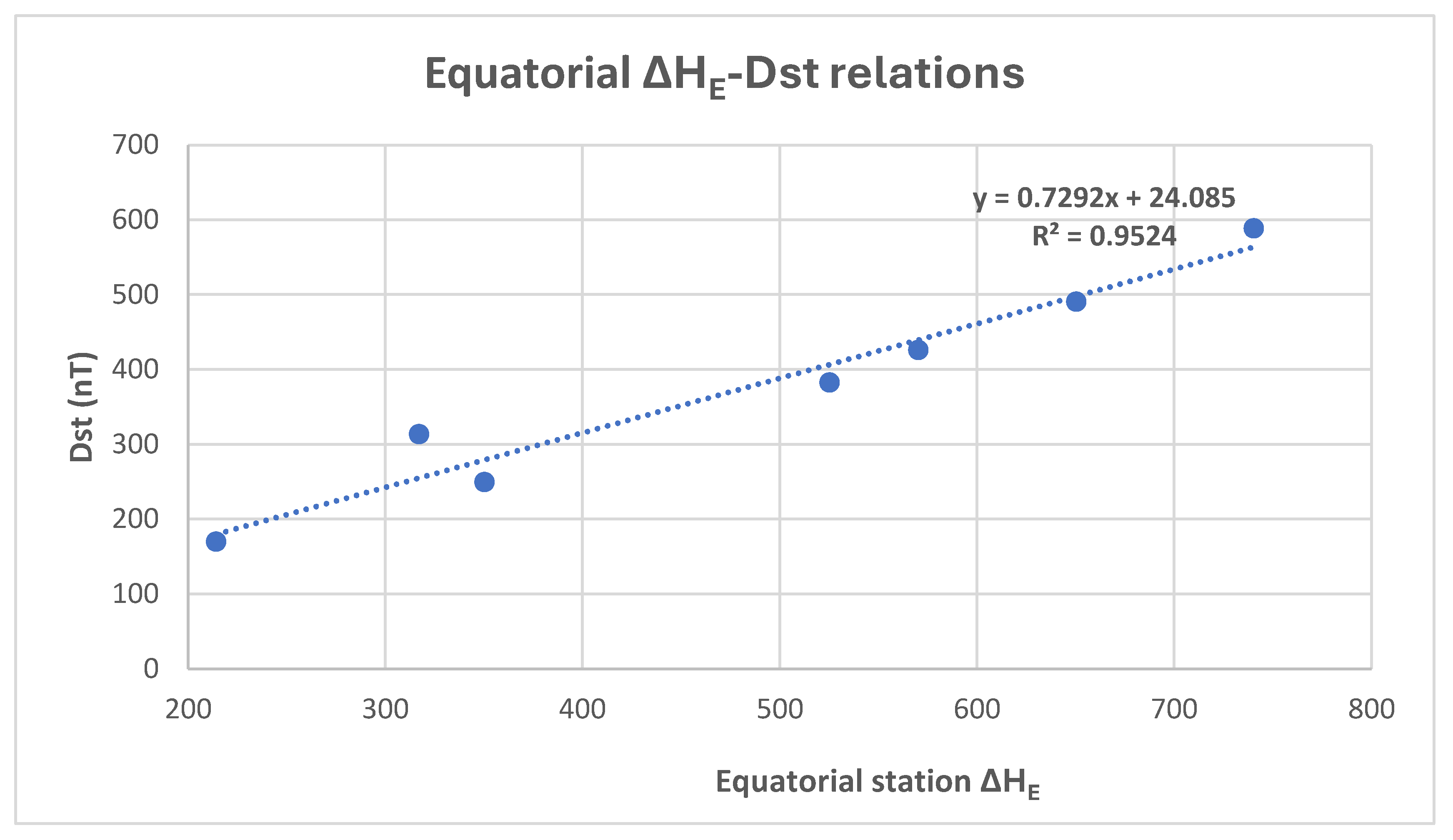
Figure 14.
Yearly mean geomagnetic aa indices for (a) the sunspot cycle 11 and (b) sunspot cycle 23.
Figure 14.
Yearly mean geomagnetic aa indices for (a) the sunspot cycle 11 and (b) sunspot cycle 23.
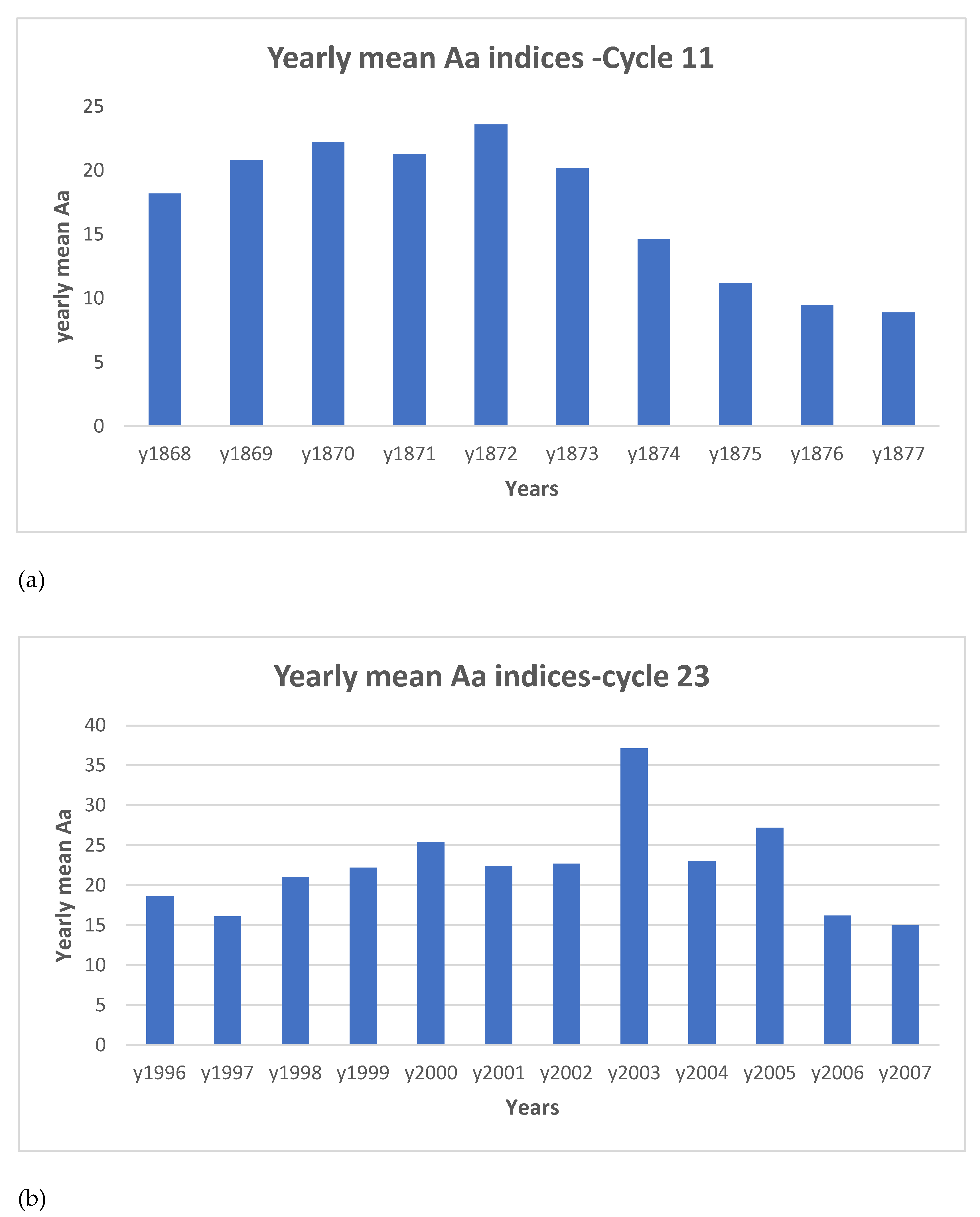
Figure 15.
Annual number of extreme space weather (ESW) events ( blue) during the sunspot cycle 19 plotted along with yearly mean classic sunspot numbers ( orange).
Figure 15.
Annual number of extreme space weather (ESW) events ( blue) during the sunspot cycle 19 plotted along with yearly mean classic sunspot numbers ( orange).
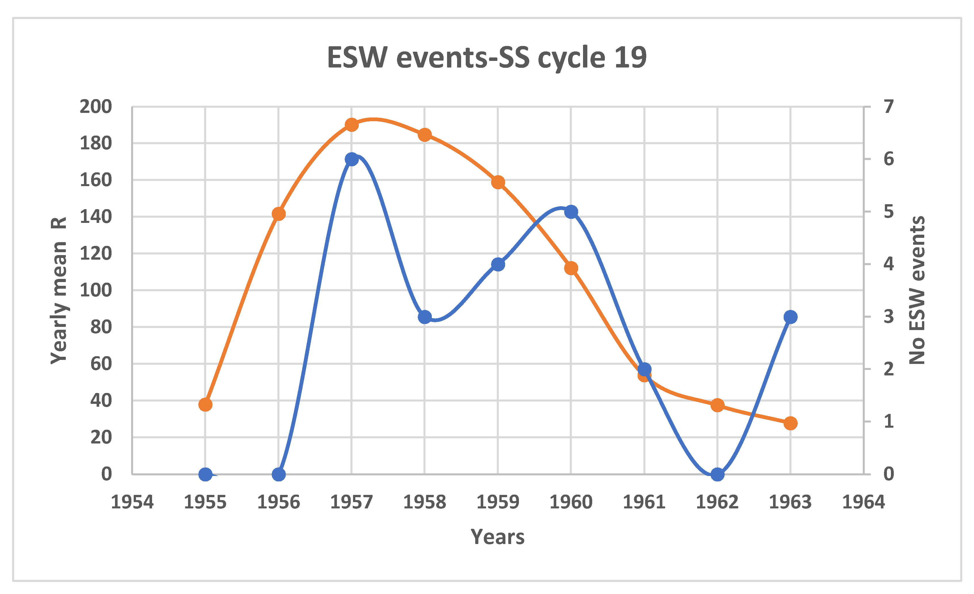
Figure 16.
Remarkable H decrease ( 752 nT) in Kodaikanal during the March 14 1989 super geomagnetic storm.
Figure 16.
Remarkable H decrease ( 752 nT) in Kodaikanal during the March 14 1989 super geomagnetic storm.
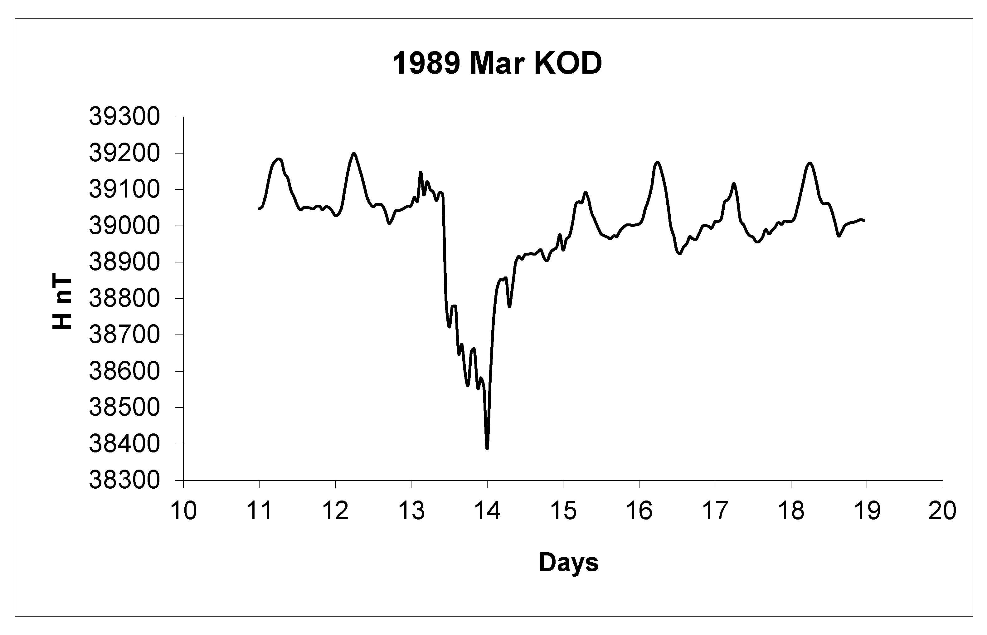
Figure 17.
Storm time deviations in hourly values of cloud cover ( %C) and magnetic declination in Trivandrum ( %D) during the Carrington storms of August 29 and September 2 in 1859 ( adopted from Eapen, 2009).
Figure 17.
Storm time deviations in hourly values of cloud cover ( %C) and magnetic declination in Trivandrum ( %D) during the Carrington storms of August 29 and September 2 in 1859 ( adopted from Eapen, 2009).
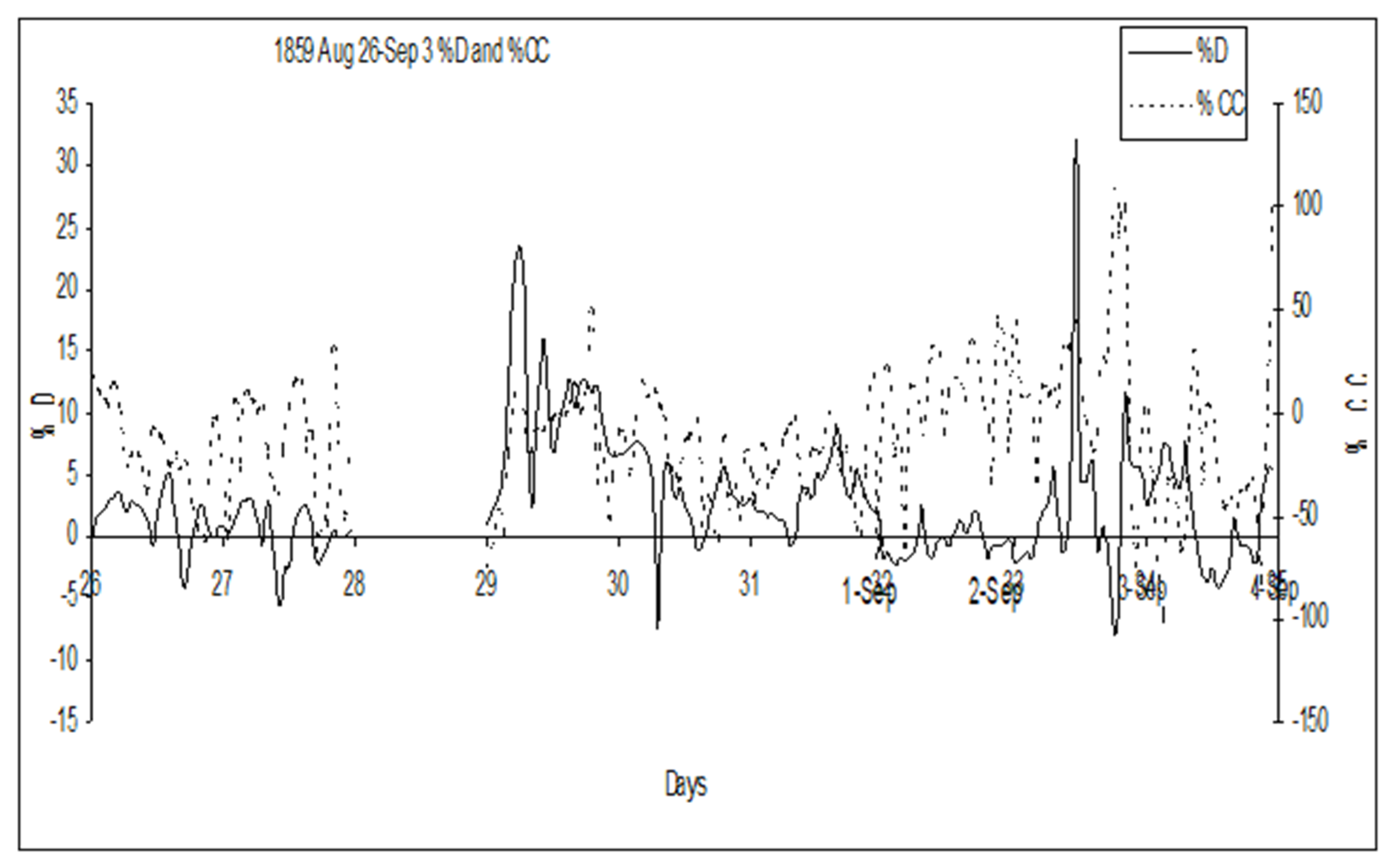
Table 3.
Observed and derived geomagnetic storm parameters in Singapore 1841-1845.
| Year | Storm Date |
GW Class |
Sing Hd | Sing Hd (BU) |
Sing ΔH (nT) |
Tvm Dst |
|---|---|---|---|---|---|---|
| 1841 | 24-Sep | G | 0.003000 | 0.0242757 | 269.16617 | 407.96638 |
| 1841 | Oct-25 | 0.001690 | 0.0137052 | 191.83450 | 250.79362 | |
| 1841 | Nov-18 | G | 0.001828 | 0.0148068 | 199.89359 | 267.17331 |
| 1841 | Dec-03 | 0.001148 | 0.0092988 | 159.59816 | 185.27486 | |
| 1841 | Dec-14 | 0.000467 | 0.0037827 | 119.24348 | 103.25597 | |
| 1842 | Jan-01 | 0.001653 | 0.0133893 | 189.52344 | 246.09650 | |
| 1842 | Feb-24 | 0.001137 | 0.0092097 | 158.94632 | 183.95003 | |
| 1842 | Jul-02 | G | 0.001422 | 0.0115182 | 175.83485 | 218.27512 |
| 1842 | Nov-10 | 0.001401 | 0.0113481 | 174.59043 | 215.74590 | |
| 1842 | Nov-21 | 0.001133 | 0.0091773 | 158.70929 | 183.46827 | |
| 1842 | Dec-09 | 0.000952 | 0.0077112 | 147.98360 | 161.66883 | |
| 1843 | Jan-02 | 0.000156 | 0.0012636 | 100.81424 | 65.79947 | |
| 1843 | Feb-06 | 0.000623 | 0.0050463 | 128.48772 | 122.04443 | |
| 1843 | May-06 | 0.001868 | 0.0151308 | 202.26391 | 271.99087 | |
| 1844 | Oct-01 | 0.000390 | 0.0031590 | 114.68061 | 93.98217 | |
| 1844 | Oct-21 | 0.000701 | 0.0056781 | 133.10984 | 131.43867 | |
| 1844 | Nov-22 | 0.000720 | 0.0058320 | 134.23575 | 133.72701 | |
| 1845 | Jan-09 | 0.001170 | 0.0094770 | 160.90184 | 187.92451 | |
| 1845 | Feb-19 | 0.000331 | 0.0026811 | 111.18439 | 86.87628 | |
| 1845 | Mar-21 | 0.000937 | 0.0075897 | 147.09473 | 159.86225 | |
| 1845 | Aug-28 | 0.007126 | 0.0577206 | 513.84237 | 905.25860 | |
| 1845 | Dec-03 | 0.000700 | 0.0056700 | 133.05059 | 131.31823 |
Table 4.
Storm time change of daily mean H in Trivandrum observatory deduced from Adies BF 1 and Adies BF 2 measurements during selected geomagnetic storms in the years 1869-1872.
Table 4.
Storm time change of daily mean H in Trivandrum observatory deduced from Adies BF 1 and Adies BF 2 measurements during selected geomagnetic storms in the years 1869-1872.
| Date of the magnetic storm |
ABF 1 Mean H (Sc Div) |
ABF 2 Mean H (Sc Div) |
Ratio of the values (ABF 1)/(ABF 2) |
|---|---|---|---|
| 1869 April 15-16 | 86.64 | 128.8 | 0.673 |
| 1869 May 13-14 | 94.772 | 148.56 | 0.67 |
| 1870 Aug 20-21 | 37 | 76.44 | 0.484 |
| 1870 Sep 24-26 | 82.63 | 143.78 | 0.575 |
| 1870 Oct 24-25 | 77.58 | 148.95 | 0.521 |
| 1871 Feb 10-11 | 84.37 | 100.288 | 0.84 |
| 1872 Feb 4 | 94.376 | 180 | 0.524 |
| 1872 Aug 15 | 98 | 170.1 | 0.576 |
| 1872 Oct 15 | 99.8 | 160.164 | 0.623 |
| 1872 Oct 17-18 | 93.86 | 161.26 | 0.582 |
| Mean Ratio | 0.6 |
Table 6.
Maximum storm time change ( %D) and daily range (Rd) found for magnetic declination observations at Trivandrum for Greenwich great geomagnetic storm periods during 1852-1869. The maximum values of Greenwich (GW) H , Helsinki (HEL) Ak and daily sunspot number corresponding to these storm dates are also given ( adapted from Eapen, 2009).
| No |
Date of Great Storm |
Maximum value of Rd |
% D Maximum |
Date & Time of %D Max |
GW H (nT) |
HEL Ak (nT) |
R |
|
|---|---|---|---|---|---|---|---|---|
| 1 | 1852 | Nov 11-14 | 5.9 | 12.98% | 1852 Nov 12, 1.30pm |
150 | 65 | 73 |
| 2 | 1853 | Jul 12-13 | 6.03 | 13.99% | 1853 Jul 13, 7.30 am |
275 | 53 | 71 |
| 3 | 1854 | Mar15-16 | 2.29 | 9.96% | 1854 Mar 16, 7.30 am |
200 | 33 | 33 |
| 4 | 1857 | May 7-8 | 5.83 | 10.69% | 1857 May11, 10.30am |
>325 | 82 | 24 |
| 5 | 1857 | Dec16-17 | 10.65 | 21.16% | 1857 Dec 17 3.30pm |
450 | 139 | 79 |
| 6 | 1858 | Apr 9-11 | 7.94 | 18.26% | 1858 Apr 10, 2.30am |
>475 | 159 | 44 |
| 7 | 1859 | Aug 28-29 | 9.83 | 21.78% | 1859 Aug 29, 6.30am |
275 | 55 | 108 |
| 8 | 1859 | Sep 2-5 | 9.43 | 32.07% | 1859 Sep 2, 8.30pm |
>>625 | 75 | 154 |
| 9 | 1859 | 13-Oct | 5.53 | 16.49% | 1859 Oct 12, 10.30pm |
>500 | 55 | 141 |
| 10 | 1860 | Aug 8-11 | 8.42 | 18.84% | 1860 Aug 8, 7.30pm |
450 | 92 | 154 |
| 11 | 1860 | Aug 12-13 | 8.88 | 17.08% | 1860 Aug 11, 4.30am |
600 | 85 | 126 |
| 12 | 1860 | Sep 6-7 | 6.62 | 16.59% | 1860 Sep 7, 12.30pm |
425 | 105 | 102 |
| 13 | 1862 | 5-Jul | 4.45 | 6.6% | 1862 Jul 5, 1.30pm |
350 | 53 | 55 |
| 14 | 1862 | Aug 4-5 | 4.1 | 11.05% | 1862 Aug 5, 4.30pm |
350 | 105 | 118 |
| 15 | 1862 | Oct 3-6 | 5.14 | 9.25% | 1862 Oct 6, 5.30pm |
425 | 109 | 40 |
| 16 | 1865 | Aug 2-5 | 6.47 | 5.63% | 1865 Aug 3, 6.30am |
500 | 123 | 90 |
| 17 | 1866 | Feb 21-22 | 5.98 | 5.63% | 1866 Feb 21, 4.30 pm |
400 | 108 | 118 |
| 18 | 1868 | 30-Sep | 4.09 | 7.91% | 1868 Oct 1 4.30pm |
200 | 56 | 64 |
| 19 | 1869 | Feb 3-4 | 3.87 | 6% | 1869 Feb 4, 11.30am |
250 | 60 | 127 |
| 20 | 1869 | Apr 15-16 | 16.34 | 12.33% | 1869 Apr 16, 6.30am |
400 | 99 | 45 |
| 21 | 1869 | May 13-14 | 12.1 | 11.13% | 1869 May 14 6.30am |
700 | 71 | 163 |
Table 7.
Maximum storm time changes in hourly magnetic declination ( %D) in Trivandrum and Dst during selected severe magnetic storm periods during the years 1981-1991 ( after Eapen, 2009).
Table 7.
Maximum storm time changes in hourly magnetic declination ( %D) in Trivandrum and Dst during selected severe magnetic storm periods during the years 1981-1991 ( after Eapen, 2009).
| Date of magnetic storm |
Date and time of maximum %D |
Value of max %D |
Max Dst (nT) |
|---|---|---|---|
| 1981 July 25 | 1981 July 25,15 hr | -6.83 | -226 |
| 1986 February 8 | 1986 Feb 8th, 22 hr | -9.91 | -307 |
| 1989 March 13-14 | 1989 Mar 13, 21 hr | -18.64 | -589 |
| 1989 Oct 20-21 | 1989 Oct 20, 7 hr | -7.04 | -268 |
| 1990 April 10-12 | 1990 Apr 12, 9 hr | -7.626 | -281 |
| 1991 March 24-25 | 1991 Mar 24, 23 hr | -8.77 | -298 |
| 1991 November 8-9 | 1991 Nov 8, 23 hr | -16.48 | -354 |
Table 8.
Deviation of storm time value daily mean H observed in Trivandrum from the respective monthly mean ( % ΔH) for selected modern storms compared with Storm time minimum Dst index.
Table 8.
Deviation of storm time value daily mean H observed in Trivandrum from the respective monthly mean ( % ΔH) for selected modern storms compared with Storm time minimum Dst index.
| storm date | % ΔH | Dst |
|---|---|---|
| 1988 Jan 14 | 20.2 | -185 |
| 1989 Feb 8 | 35.6 | -312 |
| 1991 Oct 29 | 31.8 | -251 |
| 1991 Nov 9 | 36.74 | -354 |
| 1995 Apr 7 | 14.1 | -142 |
| 1996 Oct 23 | 6.27 | -110 |
Table 10.
Number of extreme intense and super intense geomagnetic storms inferred during the sunspot cycles 8-11 inferred using low/equatorial latitude observations.
Table 10.
Number of extreme intense and super intense geomagnetic storms inferred during the sunspot cycles 8-11 inferred using low/equatorial latitude observations.
| Sunspot Cycle | No of Extreme- intense GM storms |
No of Super intense GM storms |
Total No of Severe storms |
|---|---|---|---|
| 8 ( 1841-1843) 9 ( 1844-1854) 10 ( 1855-1866) 11 ( 1867-1877) |
1 15 22 30 |
0 7 4 7 |
1 22 26 37 |
Disclaimer/Publisher’s Note: The statements, opinions and data contained in all publications are solely those of the individual author(s) and contributor(s) and not of MDPI and/or the editor(s). MDPI and/or the editor(s) disclaim responsibility for any injury to people or property resulting from any ideas, methods, instructions or products referred to in the content. |
© 2026 by the authors. Licensee MDPI, Basel, Switzerland. This article is an open access article distributed under the terms and conditions of the Creative Commons Attribution (CC BY) license.
Copyright: This open access article is published under a Creative Commons CC BY 4.0 license, which permit the free download, distribution, and reuse, provided that the author and preprint are cited in any reuse.


