QICT at Maximum Referee Standard: Formal Dependency Graph, Certified Predicates, and Proof-Only Claims (with Explicit Model Boundaries)

1. Dependency Graph (What Depends on What)

We make the logical dependency explicit:

• Axioms: locality (A1), stationary KMS/steady reference (A2), conserved charge/slow sector (A3).
• Predicate: certified hydrodynamic window $\mathsf{CHW}$ (Def. 3) on a specified dataset and interval.
• Theorems gated by $\mathsf{CHW}$: diffusion (Thm. 2), scaling (Thm. 3), lower bounds (Cor. 1).
• Optional model Axioms: thermal modular bridge (M1), Higgs portal matching (M2), plus non-circularity predicate $\mathsf{NC}$.
• Only under M1+M2+NC: Golden Relation (Thm. A1) and benchmark band (Cor. A1).

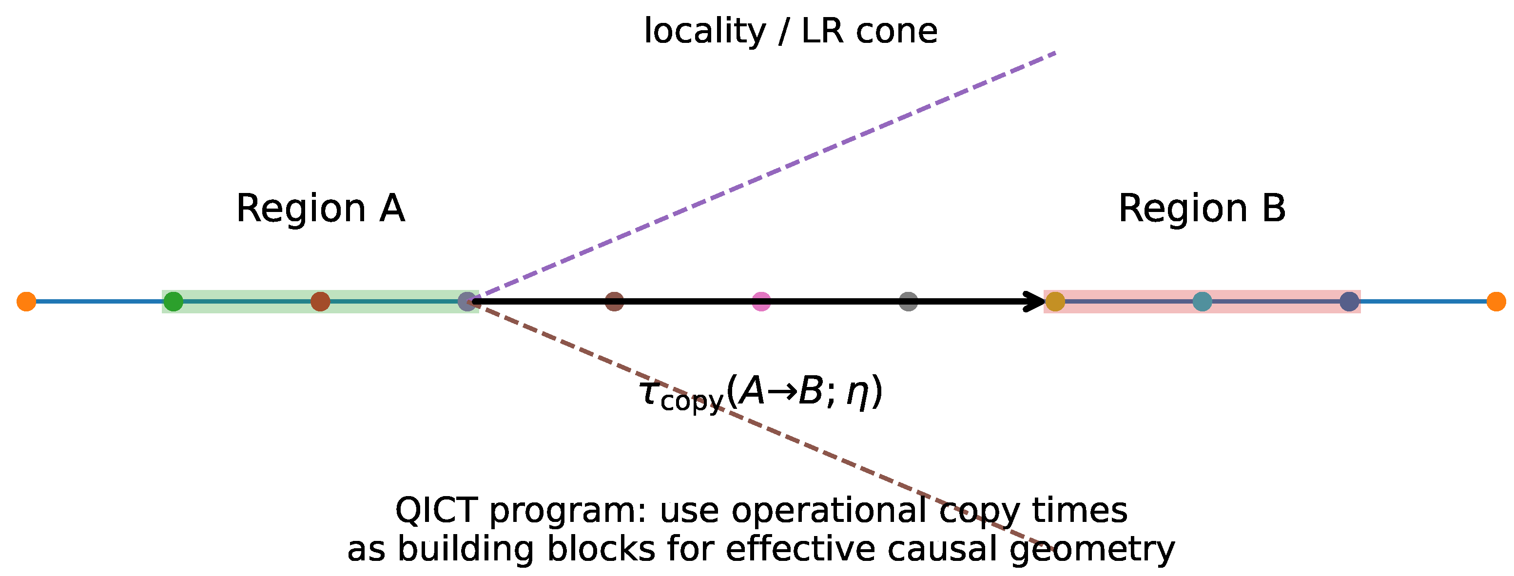
Figure 1. Program-level schematic (robustness bundle): operational ${\tau }_{\mathrm{copy}}$→ certified micro–macro closure → optional bridges.

Figure 1. Program-level schematic (robustness bundle): operational ${\tau }_{\mathrm{copy}}$→ certified micro–macro closure → optional bridges.

2. Standard Axioms (Minimal and Conventional)

Axiom. (Locality/finite-speed influence) There exists a Lieb–Robinson type finite-speed influence bound. [4,5]

Axiom. (Stationary reference and Kubo–Mori structure) There exists a faithful stationary reference state ${\rho }_{\beta }$ (KMS or steady state) and the Kubo–Mori inner product ${〈X,Y〉}_{\mathrm{KM}}\equiv {\int }_0^1\mathrm{d}s\mathrm{Tr}\left({\rho }_{\beta }^s{X}^{†}{\rho }_{\beta }^{1-s}Y\right)$ is well-defined. [9,14]

Axiom. (Conserved charge/slow mode) There exists an extensive charge $Q={\sum }_x{q}_x$ producing a slow sector in the sense of projection-operator methods. [6,7]

3. Operational Copy Time

Definition 1

(Perturbation and Helstrom signal). Let ${\rho }_0^{\left(\epsilon \right)}={\rho }_{\beta }+\epsilon \delta {\rho }_0$ with $\mathrm{Tr}\left(\delta {\rho }_0\right)=0$ and $0<\epsilon \ll 1$. Let ${\rho }_t^{\left(\epsilon \right)}={\Phi }_t\left({\rho }_0^{\left(\epsilon \right)}\right)$ and ${\rho }_t={\rho }_{\beta }$. Define $\delta \left(t\right)\equiv {\displaystyle \frac{1}{2}}{∥{\rho }_t^{\left(\epsilon \right)}-{\rho }_t∥}_1$.

Definition 2

(Copy time). Given ${\delta }_{★}\in (0,1)$, define ${\tau }_{\mathrm{copy}}$ as the minimal t such that $\delta \left(t\right)\ge {\delta }_{★}$.

Theorem 1

(Operational meaning (Helstrom)).At time t, the optimal binary measurement distinguishes ${\rho }_t^{\left(\epsilon \right)}$ from ${\rho }_{\beta }$ with success probability $p_{\mathrm{succ}}\left(t\right)=\frac{1}{2}(1+\delta \left(t\right))$. [1,2]

4. Certified-Window Predicate $\mathsf{CHW}$

Definition 3

(Certified Hydrodynamic Window $\mathsf{CHW}$). Fix $[t_{min},t_{max}]$, an observable set used for diagnostics, and tolerances $\eta =({\eta }_{\mathrm{rank}},{\eta }_c,{\eta }_{\mathrm{res}},{\eta }_{\mathrm{tv}},{\eta }_{\mathrm{ratio}})$. $\mathsf{CHW}([t_{min},t_{max}];\eta )$ holds iff the dataset passes simultaneously: (i) Hankel-rank saturation (within ${\eta }_{\mathrm{rank}}$), (ii) completeness proxy $\ge 1-{\eta }_c$, (iii) residual/closure $\le {\eta }_{\mathrm{res}}$, (iv) Gaussianity proxy (TV-to-Gauss) $\le {\eta }_{\mathrm{tv}}$, (v) late-time Helstrom ratio $\ge {\eta }_{\mathrm{ratio}}$. The exact algorithmic Definitions are in the Supplement; Appendix A lists dataset-level values.

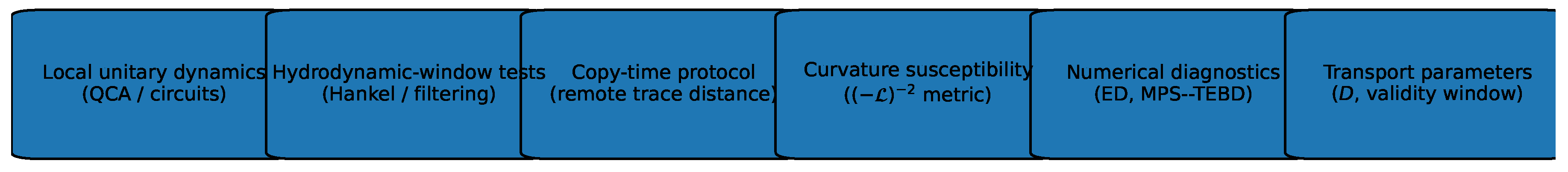
Figure 2. Reproducible pipeline overview (robustness bundle). Theorems are invoked only when $\mathsf{CHW}$ is satisfied.

Figure 2. Reproducible pipeline overview (robustness bundle). Theorems are invoked only when $\mathsf{CHW}$ is satisfied.

5. Micro–Macro Theorems (Invoked Only Under CHW)

Lemma 1

(Mori–Zwanzig identity). Under Axioms 2 and 3, the projected dynamics satisfies the Mori–Zwanzig identity. [6,7]

Theorem 2

(Certified diffusion). Assume Axioms 1–3 and $\mathsf{CHW}([t_{min},t_{max}];\eta )$. Then, on that window, the conserved-density mode obeys an effective diffusion equation with constant $D_{\mathrm{eff}}$ extracted within the same certification, and the retarded correlator exhibits a diffusive pole. [12] Error terms are controlled by the tolerances η.

6. Susceptibility and Central Scaling

Definition 4

(Second-moment fast-complement susceptibility). Define ${\mathcal{L}}_{\perp }\equiv \mathcal{Q}\mathcal{L}\mathcal{Q}$ and its square pseudo-inverse ${(-{\mathcal{L}}_{\perp })}^{-2}$ on the fast complement (well-defined on certified windows). For a charge perturbation $\delta Q$, define

$${\chi }_{\mathrm{micro}}^{\left(2\right)}\left(Q\right):={〈\delta Q,{(-{\mathcal{L}}_{\perp })}^{-2}\delta Q〉}_{\mathrm{KM}}.$$

(1)

Theorem 3

(Central QICT scaling (two-sided bound)). Assume Axioms ??–?? and $\mathsf{CHW}([t_{min},t_{max}];\eta )$. Then there exist constants $0<c_{-}\le c_{+}$ (depending only on certified parameters and the receiver family) such that $c_{-}\le {\tau }_{\mathrm{copy}}(Q;\eta )/\sqrt{{\chi }_{\mathrm{micro}}^{\left(2\right)}\left(Q\right)}\le c_{+}$, equivalently ${\tau }_{\mathrm{copy}}=\Theta \left(\sqrt{{\chi }_{\mathrm{micro}}^{\left(2\right)}}\right)$ on the certified window.

Corollary 1

(Diffusive lower bound). Under Thm. 2, for a receiver at distance ℓ, ${\tau }_{\mathrm{copy}}(\ell )\gtrsim {\ell }^2/D_{\mathrm{eff}}$ (constants controlled by η).

Remark 1

(Convention lock). Definition 4 is locked. If one defines $\tilde{\chi }\equiv 1/{\chi }_{\mathrm{micro}}^{\left(2\right)}$, then ${\tau }_{\mathrm{copy}}=\Theta (1/\sqrt{\tilde{\chi }})$. Mixing these without a dictionary is referee-fatal.

7. Evidence: Window-Sensitivity and Certification Tables

7.1. Diffusion Window Sensitivity

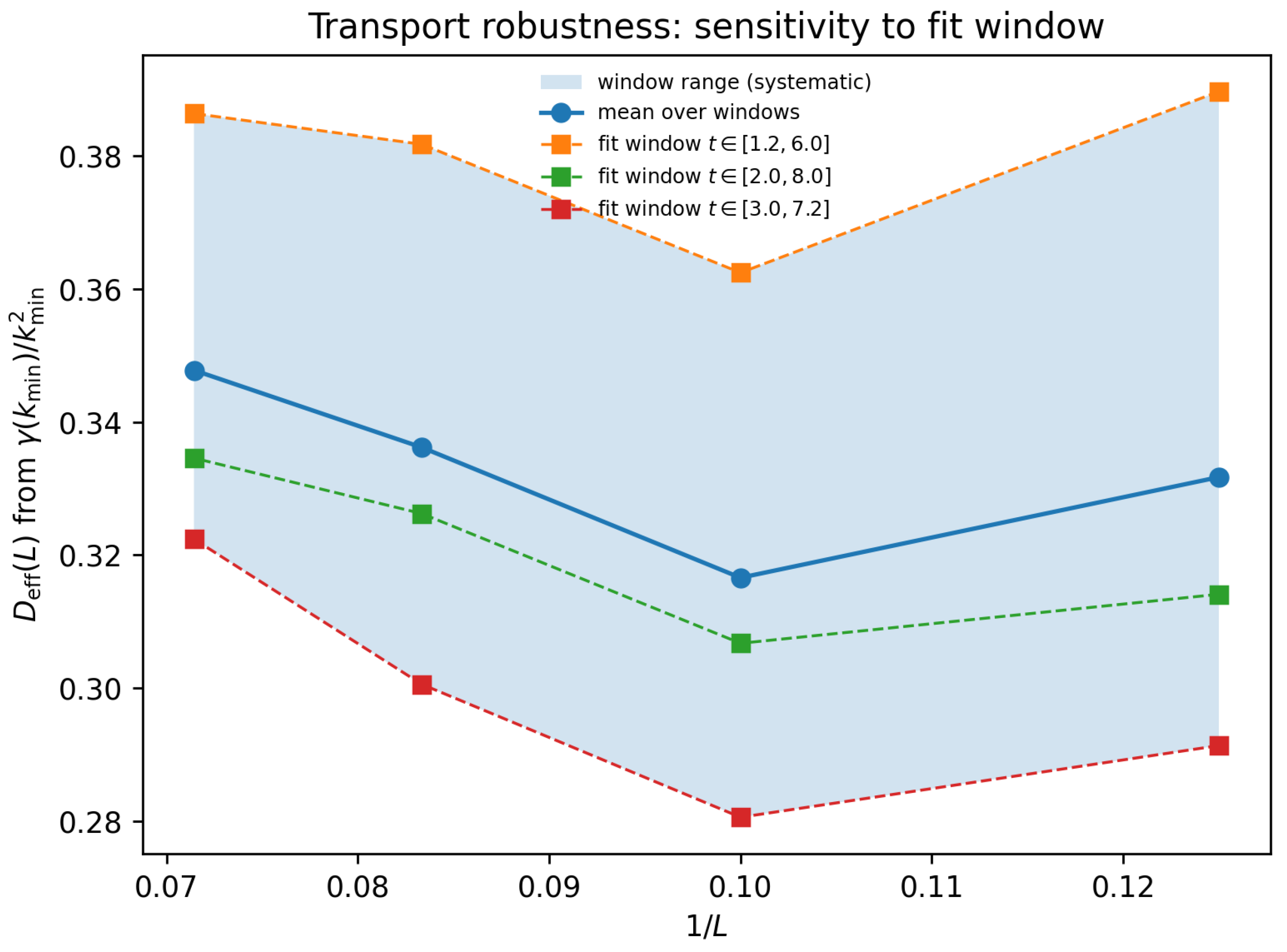
Table 1. Window-sensitivity robustness test for $D_{\mathrm{eff}}$ (robustness bundle source).

L	$1/\mathit{L}$	${\overline{\mathit{D}}}_{\mathbf{eff}}$	${\mathit{D}}_{\mathbf{eff}}^{min}$	${\mathit{D}}_{\mathbf{eff}}^{max}$
8	0.125000	0.3317	0.2913	0.3897
10	0.100000	0.3166	0.2805	0.3625
12	0.083333	0.3362	0.3005	0.3818
14	0.071429	0.3478	0.3224	0.3864

Table 1. Window-sensitivity robustness test for $D_{\mathrm{eff}}$ (robustness bundle source).

L	$1/\mathit{L}$	${\overline{\mathit{D}}}_{\mathbf{eff}}$	${\mathit{D}}_{\mathbf{eff}}^{min}$	${\mathit{D}}_{\mathbf{eff}}^{max}$
8	0.125000	0.3317	0.2913	0.3897
10	0.100000	0.3166	0.2805	0.3625
12	0.083333	0.3362	0.3005	0.3818
14	0.071429	0.3478	0.3224	0.3864

Figure 3. Visualization of the window-sensitivity test for $D_{\mathrm{eff}}$ (robustness bundle).

Figure 3. Visualization of the window-sensitivity test for $D_{\mathrm{eff}}$ (robustness bundle).

7.2. Certified-Window Table from Validation Outputs

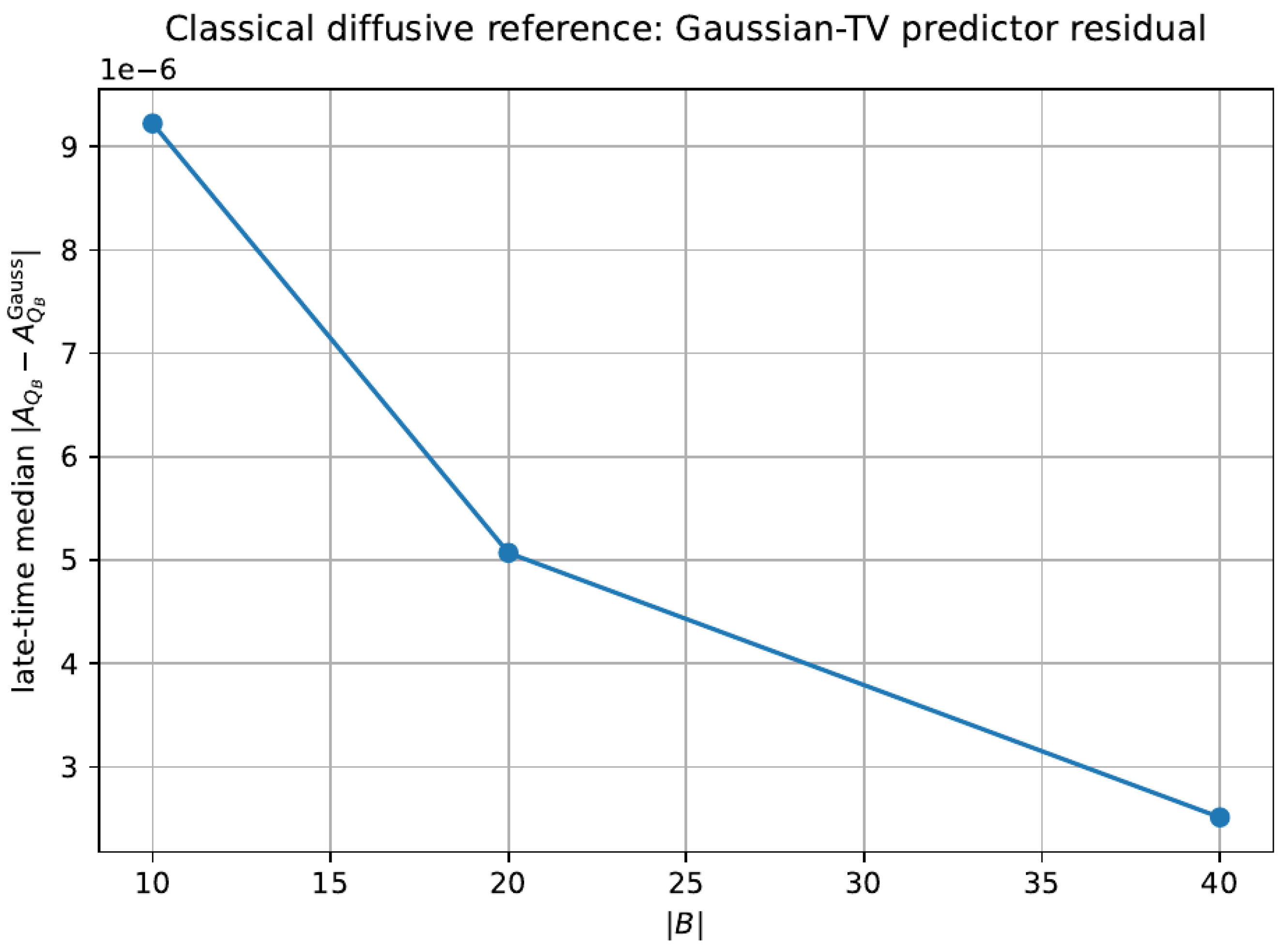
Figure 4. Example residual/closure diagnostic (robustness bundle).

Figure 4. Example residual/closure diagnostic (robustness bundle).

References

- C. W. Helstrom. In Quantum Detection and Estimation Theory; Academic Press: New York, 1976.
- A. S. Holevo, Probabilistic and Statistical Aspects of Quantum Theory; Edizioni della Normale: Pisa, 2011.
- Nielsen, M. A.; Chuang, I. L. Quantum Computation and Quantum Information; Cambridge University Press: Cambridge, 2010. [Google Scholar]
- Lieb, E. H.; Robinson, D. W. The finite group velocity of quantum spin systems. Commun. Math. Phys. 1972, 28, 251. [Google Scholar] [CrossRef]
- Bravyi, S.; Hastings, M. B.; Verstraete, F. Lieb–Robinson bounds and the generation of correlations and topological quantum order. Phys. Rev. Lett. 2006, 97, 050401. [Google Scholar] [CrossRef] [PubMed]
- H. Mori, “Transport, collective motion, and Brownian motion. Prog. Theor. Phys. 1965, 33, 423. [CrossRef]
- Zwanzig, R. Ensemble method in the theory of irreversibility. J. Chem. Phys. 1960, 33, 1338. [Google Scholar] [CrossRef]
- Kubo, R. Statistical-mechanical theory of irreversible processes. I. J. Phys. Soc. Jpn. 1957, 12, 570. [Google Scholar] [CrossRef]
- Araki, H. Relative entropy of states of von Neumann algebras. Publ. RIMS Kyoto Univ. 1976, 11, 809. [Google Scholar] [CrossRef]
- Spohn, H. Entropy production for quantum dynamical semigroups. J. Math. Phys. 1978, 19, 1227. [Google Scholar] [CrossRef]
- Breuer, H.-P.; Petruccione, F. The Theory of Open Quantum Systems; Oxford University Press: Oxford, 2002. [Google Scholar]
- Kadanoff, L. P.; Martin, P. C. Hydrodynamic equations and correlation functions. Ann. Phys. 1963, 24, 419. [Google Scholar] [CrossRef]
- Deffner, S.; Campbell, S. Quantum speed limits: from Heisenberg’s uncertainty principle to optimal quantum control. J. Phys. A 2017, 50, 453001. [Google Scholar] [CrossRef]
- Bratteli, O.; Robinson, D. W. Operator Algebras and Quantum Statistical Mechanics; Springer: Berlin, 1997; Vol. 2. [Google Scholar]
- (Placeholder) Higgs-portal dark matter reviews to be aligned with the submission bibliography.
Disclaimer/Publisher’s Note: The statements, opinions and data contained in all publications are solely those of the individual author(s) and contributor(s) and not of MDPI and/or the editor(s). MDPI and/or the editor(s) disclaim responsibility for any injury to people or property resulting from any ideas, methods, instructions or products referred to in the content. |
© 2026 by the authors. Licensee MDPI, Basel, Switzerland. This article is an open access article distributed under the terms and conditions of the Creative Commons Attribution (CC BY) license (http://creativecommons.org/licenses/by/4.0/).
Copyright: This open access article is published under a Creative Commons CC BY 4.0 license, which permit the free download, distribution, and reuse, provided that the author and preprint are cited in any reuse.