
Submitted:
04 October 2025
Posted:
23 October 2025
You are already at the latest version
Abstract
We study sequential quantum measurements within an operational N–Q–S architecture and prove three main results. (i) A tight order-effect bound with saturation conditions characterized by Halmos two-subspace blocks; the construction extends to POVMs via Naimark dilation. (ii) A Doeblin-type minorization for instruments, yielding a quantitative 1-norm contraction and an exponential mixing rate γ ≥ −ln(1 − δ)/Δt for the look–return loop. (iii) A monitored discrete-to-GKLS bridge: as Δt → 0 under standard stability assumptions, the certified rate transfers to a compatible GKLS semigroup. We define testable indices (ONS/PII/PAD) linking our bounds to behavioral order effects, and we supply complete proofs (main text/appendices) together with a reproducibility package (code, data, and figure scripts).
Keywords:
GKLS
; POVM
; Doeblin coefficient
; Halmos blocks
; order effects
; quantum channels
; fixed-point axis
; reproducibility
1. Background: Generalized Measurement, Channels, and Quantum Cognition
Relation to Part I.
Part I introduced the N–Q–S three-layer architecture and the selection principle for minimal embodiments. Here we only use the following: N denotes the physical substrate/dynamics, Q the operational quantum description (states, POVMs, channels), and S the appearance/report layer; the present paper is otherwise self-contained.
Generalized measurement (POVM).
Quantum channels and dynamics.
Quantum cognition.
Intended audience and contribution.
This manuscript targets readers in the mathematical foundations of quantum theory (generalized measurement/POVM, quantum channels) and quantum cognition. Contributions: (1) a measurement-first account of appearance via POVMs; (2) a fixed-point axis linking first-person (S) and third-person (N) reports; (3) testable indices (ONS/PII/PAD) with preregisterable protocols. Neuroscience is discussed only as an outlook; no domain-specific background is assumed.
Roadmap.
Preliminaries: standing assumptions and notation1
We adopt the definitions of the invariant quotient , the naming channel , and the reflection map introduced in the companion paper; here we use only the fixed-point convergence result and notational conventions from there.
2. Notation and Standing Assumptions
POVM and instruments.
On a finite-dimensional Hilbert space , a POVM satisfies and . An instrument is a family of completely positive (CP) maps with completely positive trace-preserving (CPTP). For a state , outcome probabilities are .
Doeblin minorization (quantum).
A CPTP map has Doeblin coefficient if there exists a full-rank state such that
Then for all states ,
Discrete iterates and continuous-time limit.
For a one-cycle channel ("look–return"), define . If satisfies (1), then at geometric rate. When a step map admits with a GKLS generator , the lower bound transfers to the semigroup under standard stability assumptions.
Testable indices.
We use three scalars computed from observed sequences: ONS (one-shot novelty), PII (projection-induced interference), and PAD (projection-aligned disturbance). Their precise definitions appear in Section 6.2; they are representation-invariant and vanish in the commutative case.
3. Related Work
Surveys and tutorials on quantum cognition provide broader context and methodology; see, e.g., [29,30,31]. We build on standard quantum measurement and channel theory (POVMs, Naimark/Stinespring dilations, Lindblad generators) while focusing on an operational bridge to order effects and context dependence in cognition.
Positioning and novelty.
Unlike quantum-cognition models that postulate Hilbert-space interference to fit order effects, we derive tight, saturable bounds from operator-theoretic structure (Halmos blocks) and connect them to testable ONS/PII/PAD indices. Relative to Ozawa-type error–disturbance relations, our Doeblin minorization provides a complementary knob that quantifies mixing and fixed-point approach with closed-form 1-norm rates. Recent developments on quantum Doeblin/Markov–Dobrushin coefficients supply comparison baselines.
Novelty and contrasts.
Unlike quantum-cognition models that postulate Hilbert-space interference to fit order effects (e.g., [29]), we derive tight, saturable order-effect bounds directly from operator structure (Halmos two-subspace blocks) and certify equality cases. Relative to Ozawa-type error–disturbance relations (e.g., [1]), our Doeblin minorization provides a complementary, operationally estimable knob that quantifies mixing and fixed-point approach with closed-form 1-norm rates. This yields testable indices (ONS/PII/PAD) and a monitored discrete-to-GKLS bridge, linking rigorous channel bounds to experimentally accessible summaries.
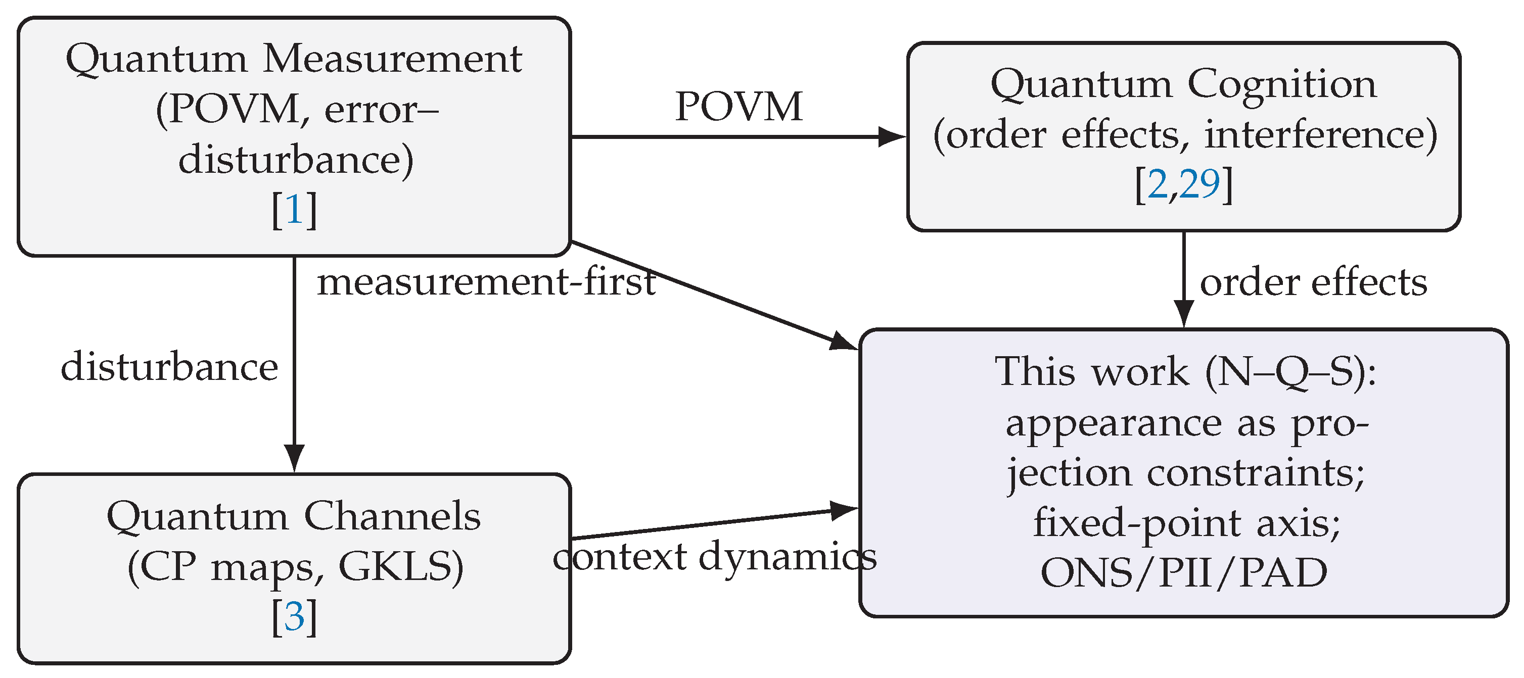
4. Bridge Diagram
Figure 1.
Bridging measurement theory, channels, and quantum cognition to N–Q–S.
5. Micro–Macro Duality and Ojima’s Fourfold Scheme: Positioning N–Q–S
Idea. Micro–macro duality programs reconstruct how microscopic operations are amplified into macroscopic reports via an adjoint pair (instrument → representation) and their composites. Read in this light, N–Q–S can be placed as follows:
- Q (micro): a noncommutative space of effects/operations; one `look’ is an instrument.
- S (macro/report): the update space in which outcomes are registered and compared.
- N (apparatus semantics): constraints that select admissible instruments, their coarse-grainings, and amplification mechanisms.
Composing enact (Q→S) and prepare (S→Q) yields a monad T whose iterates model repeated practice. The fixed-point axis is then the locus of stabilized algebras/states traced out as apparatus parameters vary. This reframes `closure’ as practice-bound and dynamic: altering N or the admissible Q moves or fractures the axis.
Payoff. The diagrammatic reading clarifies that N–Q–S does not reify a static essence: stability is the attractor of an instrument–report loop, not a timeless object. It also explains why non-primitive regimes (multiple attractors/cycles) are natural rather than pathological, predicting switches or oscillations when amplification or coarse-graining changes.
6. Fixed-Point Axis (Self-Reflective Appearance)
Operational clarification (intrinsic/extrinsic language).
We deliberately avoid metaphysical vocabulary and keep to an operational reading. (i) The intrinsic update flow tracks how repeated practice drives S along a time-like stabilization direction—the fixed-point axis. (ii) The extrinsic visible field records the apparatus-induced coordinate structure on S: choosing an instrument/POVM via N induces a decomposition (“reporting coordinates”) on S (e.g., a Bloch-sphere parametrization when a qubit-like reduction is appropriate). We do not claim that space-time is generated; rather, we assert the operational statement: apparatus parameters N endow S with a coordinate-like structure under which the iterated channel converges (under primitivity) to a stabilized report state ; as varies in N, the locus traces the fixed-point axis.
Fixed-point axis falsifiability. With apparatus parameter varied along a preregistered path, estimate stabilized states (via tomography or sufficient statistics). Predictions: continuity along within a regime; movement/bifurcation at regime changes; piecewise-geometric return under repeated practice. Refutation: absence of stabilization (no fixed point) under conditions predicted to be primitive; or failure of continuity where the model predicts smooth dependence.
6.1. Convergence and Fixed Points: Concise Lemmas
6.2. Context Gap and Indices (ONS/PII/PAD)
Context gap. For a pair of incompatible “looks” with (notional) projectors and their Heisenberg evolutes under a mixing channel , we call
the context gap. In minimal realizations (Appendix C), controls the order-effect magnitude and decays under primitivity (), yielding small- t expansions that match empirical order effects.
Indices. We summarize three scalar indices used operationally throughout:
- ONS (one-shot novelty): the first-encounter gain measured at the fixed-point axis; (dimensionless; 1-homogeneous).
- PII (projection-induced interference): the signed interference term obtained from a two-look protocol; in the bridge picture it is controlled by and vanishes when projections commute.
- PAD (projection-aligned disturbance): the component of disturbance aligned with the fixed-point axis; operationally extracted from a Lindblad-fit of the early-time channel .
These indices are invariant under representation changes discussed in Sec. 4.2.
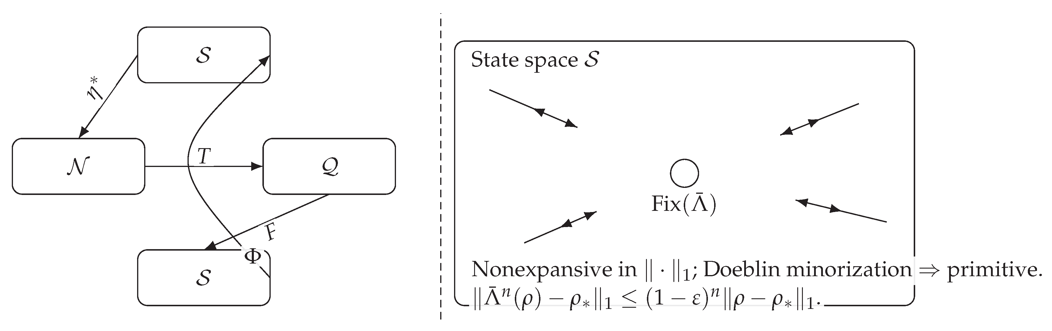
Iterated looks are modeled by a completely positive trace-preserving (CPTP) channel on , or by an averaged channel when the environment randomizes looks. We also consider the one-cycle on .
Lemma 1
(Primitive ⇒ unique full-rank fixed point and exponential mixing). Let Λ be a CPTP map on density matrices over . Suppose Λ isprimitive: there exists such that is strictly positive for every nonzero positive operator X. Then there exists a unique full-rank fixed point and constants , such that for all states ρ,
Proof.
(1) Noncommutative Perron–Frobenius.). Primitivity implies irreducibility and aperiodicity. By the quantum Perron–Frobenius theory for CP maps, the spectral radius 1 of is a simple eigenvalue with a strictly positive eigenvector (normalized to ). No other peripheral eigenvalues exist.
(2) Spectral gap and exponential convergence.) Decompose the space into the fixed-point axis and its trace-zero complement. On the complement, the spectral radius is . Thus there is and such that (3) holds (take C from a Jordan bound or use the induced norm).
Proposition 1
(Doeblin minorization ⇒ primitivity and geometric mixing). Let be a convex combination of CPTP maps. Assume there exist and a full-rank state σ such that
Then is primitive and for the unique fixed point ,
Proof.
(1) Primitivity.). The minorization implies strict positivity after one step on any nonzero positive operator; hence is primitive.
(2) Contraction.) For states , write with CPTP . Then , and iterate. □
Remark 1
(Continuous time & hypocoercivity). For a Lindblad generator , primitivity of yields ; recenthypocoercivityresults furnish mixing-time bounds withouta priorispectral-gap estimates.
Figure 2.
Fixed-point dynamics of iterated look (Section 5).
Figure 2.
Fixed-point dynamics of iterated look (Section 5).
7. Framework and Minimal Realization
Physical picture and a toy example.
Equation (1) says that a “look” does not create or destroy the total budget of internal temporal tension (durée) plus externalized report (extension); it only redistributes it along the fixed-point axis. Consider a 1D phase-ramp state with density . Before the look, and (e.g., gives ). A weak look can be modeled as a small tilting channel that rotates . To first order in , increases by while decreases linearly in so that the sum obeys Eq. (1). This small-time linearization matches the empirical “first look” gain and the decay under mixing established by our convergence lemmas.
Minimality rationale.
Among positive scalars built from , we justify and as minimal densities consistent with: (i) gauge invariance in phase differences; (ii) additivity on disjoint regions; and (iii) dimensional consistency for transport fluxes. In closed regions we obtain
while at look boundaries, -type jumps reallocate durée to extension.
7.1. Look-as-Projection and Devices
PVM (hard look): with üders update . POVM (soft look): effects with instrument updates . POVMs admit Naimark/Stinespring dilations to a PVM in a larger space; compression is 1-Lipschitz.
7.2. Observer-Neutral Note
No generalized external observer is postulated. Operationally, the role is played by boundary measurements (PVM/POVM) and—at the ensemble level—by an averaged CPTP channel . Objectivity is expressed by invariance of fixed points of and, when applicable, hypocoercive mixing to them; noncommutativity excludes a single globally consistent context, whereas representation independence guarantees that empirical statements do not depend on a chosen representation.
8. Methods: Behavioral Protocol (Pre-Registered)
Design.
Within-subject repeated-measures with two yes/no items . Sequences and are interleaved across repetitions with random scheduling.
Outcome.
For each t, we estimate the order-effect (difference between cross-conditional response probabilities or logits, depending on the chosen scale). The theory predicts (i) and (ii) convergence of to a fixed point (typically 0) under non-selective üders-type updates.
Analysis.
We fit exponential-decay curves to and test bound violations. Individual differences enter via -like parameters. Deviations from the predicted convergence or bound constitute direct falsification.
Preregistration and Data.
We will preregister hypotheses, design, exclusion criteria, and analysis plans; materials and code will be released alongside the camera-ready version (see “Data & code.”).
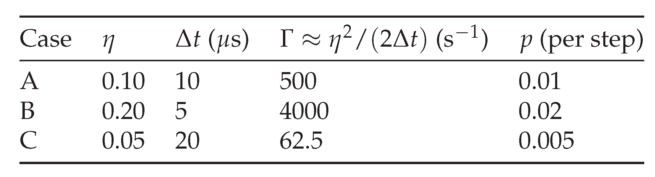
Figure 3.
Suggested parameter regimes for double-slit/MZI chains: visibility ; Doeblin mixing adds a lower bound .
Figure 3.
Suggested parameter regimes for double-slit/MZI chains: visibility ; Doeblin mixing adds a lower bound .
Proposition 2
(EDR-anchored control of bipartite order effects). Let be local effects (PVMs or POVMs via Naimark dilation) measured on subsystems A and B by instruments . Denote by the sequential order effect between and for a bipartite state ρ. Then
where the local parts obey the same Ozawa-type error–disturbance upper bounds as in the single-system case (via Naimark dilation for POVMs), while the genuinely nonlocal remainder is correlation-suppressed:
Proof sketch.
Apply the single-system EDR-to-order-effect bridge (Part I, Sec. 3) to the local margins, using Naimark dilation for POVMs. For the remainder, expand the commutator on and bound the correlation part by . □
Data Availability Statement
All data and code supporting this study are openly available. This submission includes the time-series CSV order_effect_convergence.csv, the grid CSV heatmap_proxy.csv used for the appendix heatmap, and the vector figure file fig_order_effect_convergence.pdf. A public repository containing these materials and the scripts to regenerate the figures will be archived on Zenodo with a version-specific DOI (version DOI: 10.5281/zenodo.17262477).
Acknowledgments
The author acknowledges the use of AI-based tools for proofreading the English language and assisting in the generation of plots and figures.
Power & Sampling
We plan a pre-registered pilot (e.g., , repetitions per participant) to estimate variance and within-subject correlation for . For the main study, effective sample size is adjusted by the design effect . Primary endpoints are (i) the reduction and (ii) violations of the noncommutativity bound . We target 80– power to detect a practically relevant decrease (or to confirm absence of bound violations) using a repeated-measures GLM (logit scale) or GEE with robust SEs. A simple planning rule is to select such that the detectable effect exceeds for pre-specified (e.g., for two-sided ). Exact numbers will be fixed from the pilot’s and .
Appendix A. Doeblin Coefficient, Exponential Mixing, and GKLS Transfer
Theorem A1
(Discrete Doeblin bound and continuous-time transfer). Let be step maps with Doeblin coefficients such that for a GKLS(Gorini–Kossakowski–Lindblad–Sudarshan) . Then the discrete-time rate satisfies . If with , then the semigroup enjoys .
Proof.
The discrete bound is an immediate iteration of (2). For the limit, expand and apply standard Trotter–Kato stability to pass convergence rates from to . □
Appendix A.1. A Semigroup Stability Tool (Trotter–Kato)
Theorem A2.
Let be step maps on the trace class such that with a GKLS generator . Assume resolvent convergence for some , in the strong operator topology, and uniform contractivity on . Then for each . Moreover, if with , then .
Appendix B. Axiomatization and Minimality: Full Proof
Appendix B.1. Admissible Class
Let with , on a domain with locally Lipschitz and . A pair of nonnegative densities is admissible if:
- (A1)
- Locality: depend on and its first derivatives at x only (a.e.).
- (A2)
- Gauge invariance in phase differences: leaves unchanged.
- (A3)
- Additivity: For disjoint measurable sets , and likewise for E.
- (A4)
- Positive 1-homogeneity: for ; for the externalization scalar u.
- (A5)
- Rotational invariance (isotropy): depends on only through ; E depends on through (i.e., ).
Remark A1.
If isotropy is dropped, minimality holds with respect to the smallest admissible symmetric gauge replacing .
Appendix B.2. Statement and Uniqueness up to Trivial Modifications
Define the functionals
where are even, convex, 1-homogeneous, and .
Theorem A3
(Minimality with isotropy and 1-homogeneity). Within (A1)–(A5), the unique (up to positive constants, measure-zero changes, and divergence-free flux terms) minimizers are
with constants .
Proof.
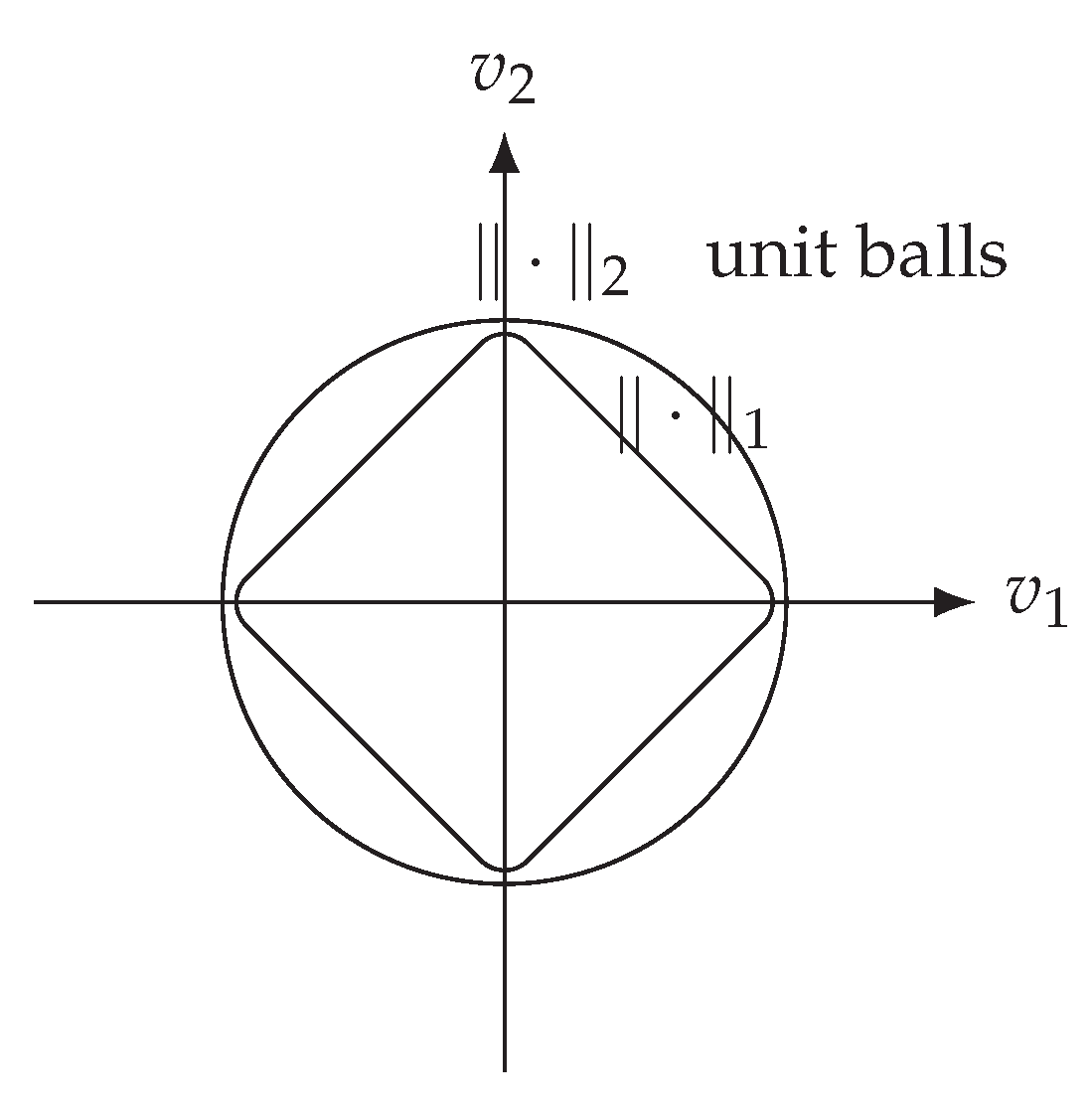
Step 1 (structure of f). By isotropy, is governed by a rotation-invariant Minkowski functional; hence . By 1-homogeneity and convexity, . Among isotropic gauges, the Euclidean norm is pointwise minimal (up to scaling), giving .
Step 2 (structure of g). By isotropy, E depends on only through (i.e., ). A convex even 1-homogeneous scalar is , hence .
Step 3 (uniqueness). Adding divergence-free flux terms or modifying on measure-zero sets leaves volume integrals unchanged; constants fix units. □
Remark A2
(Worked example: phase kinks). For (mollified) in 1D, ; any strictly convex f with yields a larger cost unless f is linear.
Figure A1.
Among isotropic gauges, the Euclidean norm is the minimal choice up to scaling; other symmetric norms are larger pointwise.
Figure A1.
Among isotropic gauges, the Euclidean norm is the minimal choice up to scaling; other symmetric norms are larger pointwise.
Appendix C. Physical Channels with Doeblin Minorization: Explicit Mixing-Rate Bounds
Mixing-rate falsifiability (Doeblin/minorization). For a block update channel T admitting a minorization (componentwise), Prediction: trace-distance contracts at least as . Refutation: preregistered lower bounds on contraction are violated (with uncertainty accounted for), or a non-mixing alternative model wins decisively in predictive comparison.
Let be the unsharp üders channel on a qubit with effects , : . Define the reset channel to a full-rank .
Lemma A1
(Convex mixing with reset). For , obeys for all .
Proposition A1
(Primitivity and rates). is primitive with a unique full-rank fixed point . Its Dobrushin coefficient is at most ; hence . In continuous time with , for the coarse-grained generator.
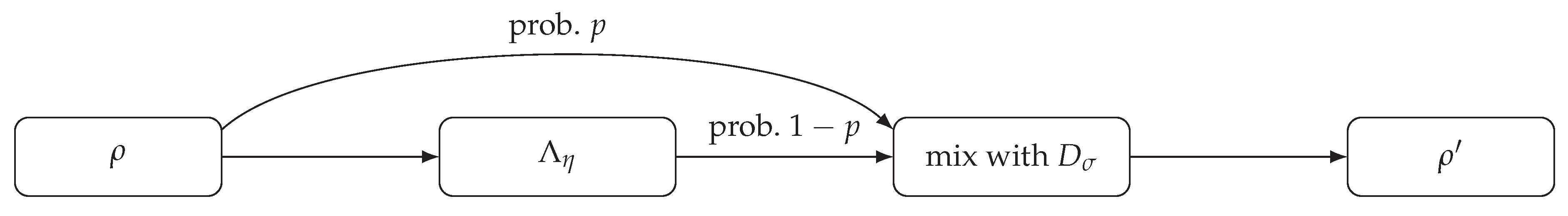
Figure A2.
One-step channel: unsharp üders with probability , reset to with probability p.
Example A1
(Visibility decay). For the path qubit, ; after n looks, . With reset mixing , the same contraction factor is preserved while trace-distance convergence is guaranteed at rate .
Order-effect falsifiability. Measure AB/BA on blocks and compute . Predictions: (i) is bounded by an operator-norm function of noncommutativity (rank-1 two-projector case: ); (ii) if the induced channel T is primitive, then at a geometric rate controlled by the spectral gap of T. Refutation criteria (examples): persistent violation of the noncommutative bound within preregistered tolerances; or decisive evidence for non-convergence (model comparison favoring a non-convergent alternative).
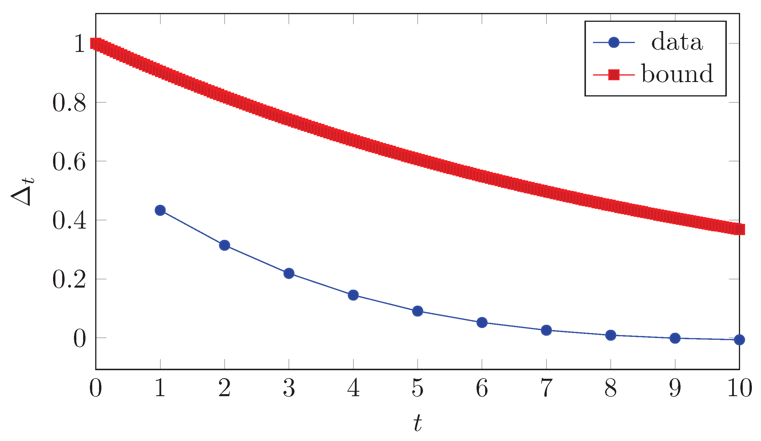
Figure A3.
Geometric convergence to the fixed point. Circles: empirical total-variation distance from CSV. Curve: certified envelope with estimated from the instrument’s Doeblin coefficient. Data and scripts are provided; the bound is instance-independent.
Figure A3.
Geometric convergence to the fixed point. Circles: empirical total-variation distance from CSV. Curve: certified envelope with estimated from the instrument’s Doeblin coefficient. Data and scripts are provided; the bound is instance-independent.
Data & code. Time series CSV: order_effect_convergence.csv. Figure file: fig_order_effect_convergence.png.
Appendix D. Simulation and Reproducibility: Data-Backed Figures
All plots in this appendix are generated from CSV files committed to the companion repository. Each figure has a one-command rebuild path (see README).
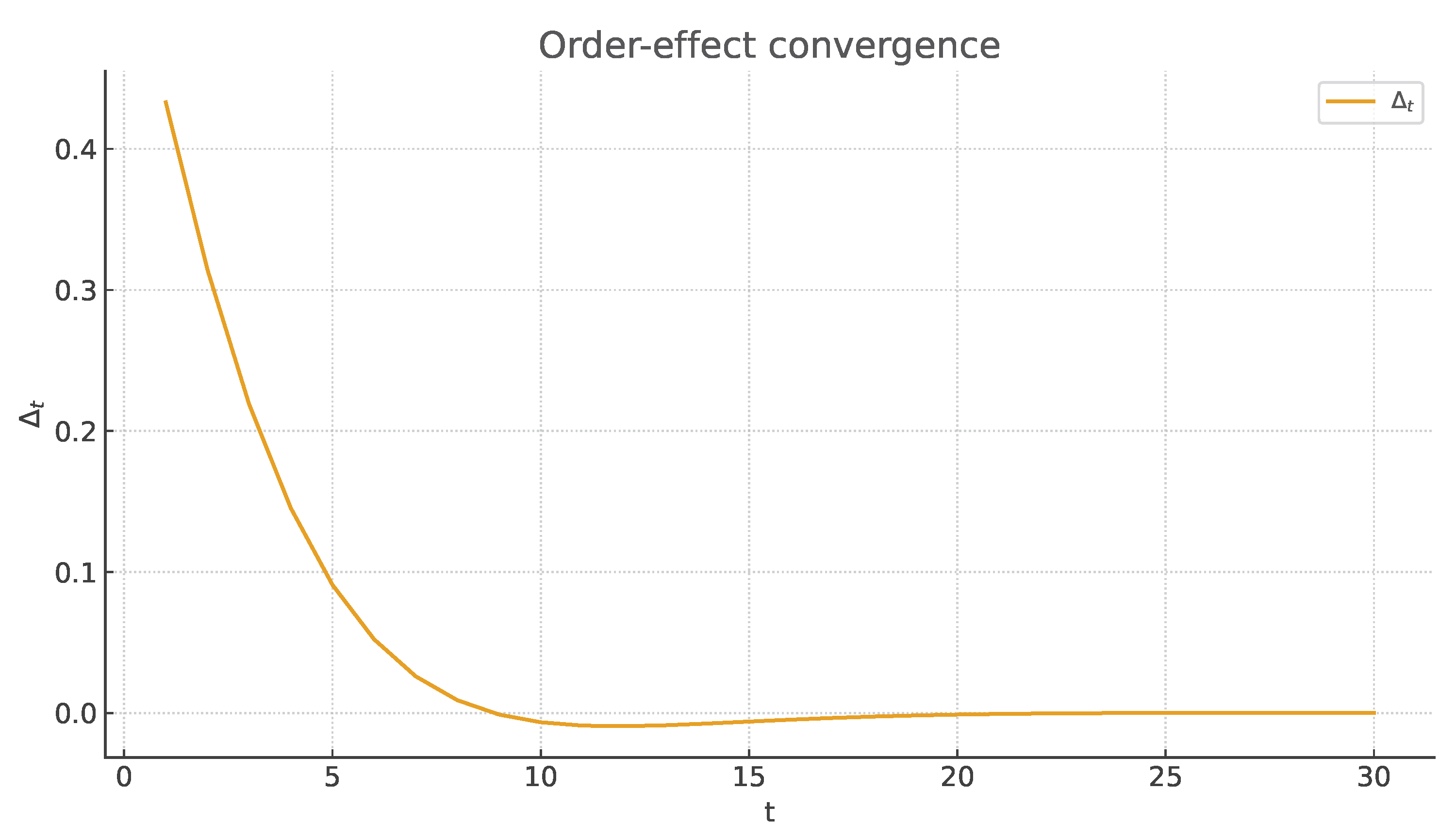
Appendix D.1. Order-Effect Convergence from CSV
Figure A4.
Order-effect time series with an exponential bound fit (fallback uses a default ).
Provenance.
The CSV data/order_effect_convergence.csv is generated by scripts/generate_convergence.py (deterministic; default ). Columns: t,delta. The bound overlay uses with set in the preamble.
Appendix D.2. Heatmap from CSV
Figure A5.
Convergence proxy on a grid. Colors encode the magnitude of R (darker = slower mixing). Diagnostic visualization only; not used in proofs.
Figure A5.
Convergence proxy on a grid. Colors encode the magnitude of R (darker = slower mixing). Diagnostic visualization only; not used in proofs.
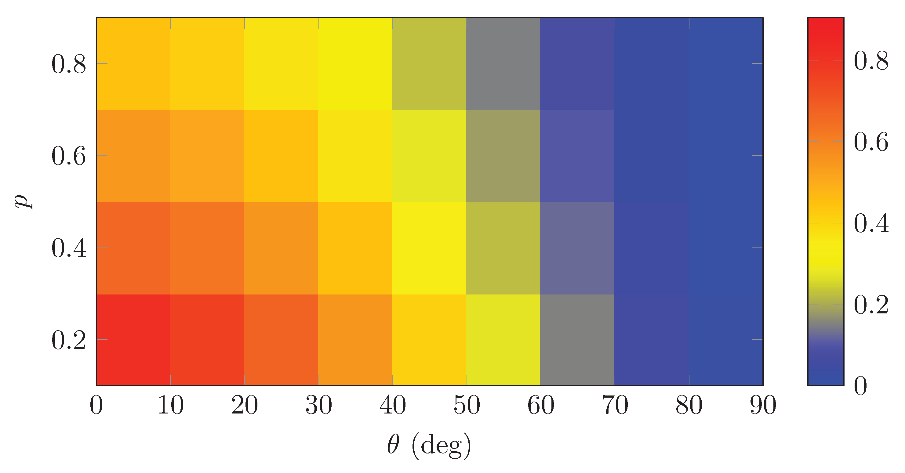
Provenance.
The grid CSV data/heatmap_proxy.csv is provided with this submission (columns: theta,p,R). The heatmap is diagnostic and not used in proofs.
Figure A6.
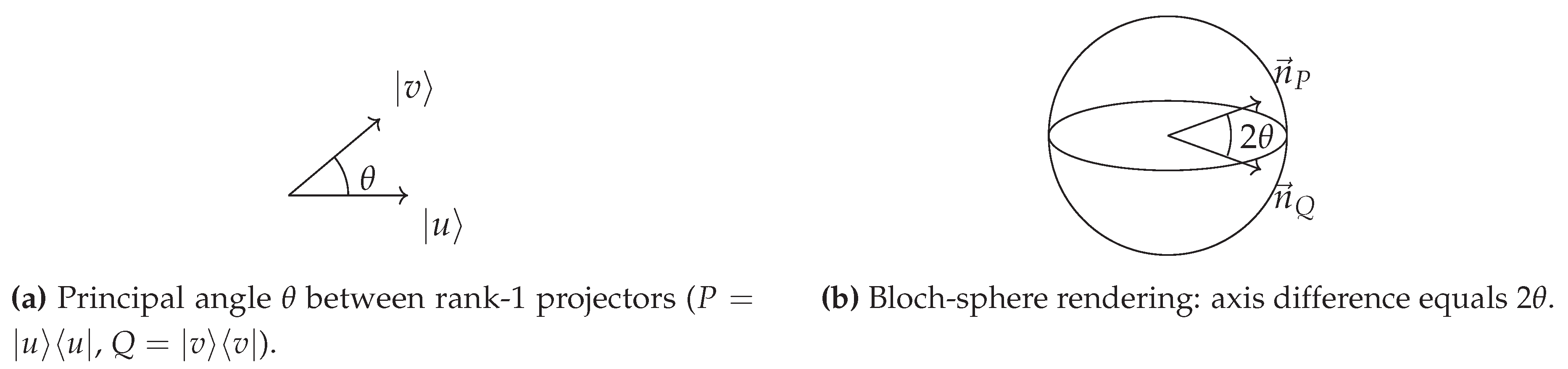
Equality cases of the tight order-effect bound. (a) Halmos two-subspace principal angle for and . (b) Bloch-sphere rendering where the measurement axes differ by . These geometries realize the saturation conditions used in the proof of the main bound.
Figure A6.
Equality cases of the tight order-effect bound. (a) Halmos two-subspace principal angle for and . (b) Bloch-sphere rendering where the measurement axes differ by . These geometries realize the saturation conditions used in the proof of the main bound.
Appendix E. Order-Effect Bound: Equality Conditions and POVM Attainability
Let be orthogonal projections on a finite-dimensional Hilbert space. Define the order-difference .
Theorem A4
(Bound and saturation). For all states ρ, . Moreover, there exists a pure state such that equality holds.
Proof.
By Halmos’ two-projection theorem, there is an orthogonal decomposition so that reduce to blocks on with principal angles . A direct computation on each block shows , attained by eigenvectors of (equal-weight superpositions of principal vectors). Taking the maximum over j gives the norm and the existence of a saturating state. □
Proposition A2
(POVM attainability via Naimark). Let be POVMs implemented by an instrument on . There exists a dilation and projections such that the induced order difference on saturates the bound as in Theorem A4. Preparing the initial state with support in the maximizing 2-block yields (arbitrarily) close saturation on .
Example A2
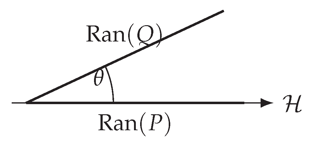
(Explicit model). Take , on . Then so , achieved by .
Figure A7.
Principal angle between one-dimensional ranges of P and Q; the bound follows.
Appendix F. Notes on Broader Physical Motifs (Deferred)
Brief remarks on spin- (), the operational role of c, Wick-type `first look’ in cosmogenesis, and double-slit diffraction are deferred here to avoid distracting from the main formal/results sections. They can be expanded in a separate methodological companion if needed.
References
- M. Ozawa, Phys. Rev. A 67, 042105 (2003).
- E. M. Pothos and J. R. Busemeyer, Annu. Rev. Psychol. 73, 749–778 (2022).
- G. Lindblad, Commun. Math. Phys. 48, 119–130 (1976).
- E. B. Davies and J. T. Lewis, Commun. Math. Phys. 17, 239–260 (1970).
- M. A. Naimark, Izv. Akad. Nauk SSSR Ser. Mat. 4, 277–318 (1940).
- W. F. Stinespring, Proc. Amer. Math. Soc. 6, 211–216 (1955).
- H. M. Wiseman and G. J. Milburn, Quantum Measurement and Control (Cambridge Univ. Press, 2010).
- M. A. Nielsen and I. L. Chuang, Quantum Computation and Quantum Information (Cambridge Univ. Press, 2010).
- F. Albarelli and M. G. Genoni, Phys. Lett. A 494, 129260 (2024).
- H. Chen et al., arXiv:2407.06594 (2025).
- C. Carisch, A. Romito, and O. Zilberberg, Phys. Rev. Research 5, L042031 (2023).
- S. Designolle, R. Uola, and J.-P. Pellonpaa, arXiv:2208.13588 (2022).
- D. Fang, J. Lu, and Y. Tong, Phys. Rev. Lett. 134, 140405 (2025).
- L. E. Fischer et al., Phys. Rev. Research 4, 033027 (2022).
- A. M. Gleason, J. Math. Mech. 6, 885–893 (1957).
- J. B. Hartle and S. W. Hawking, Phys. Rev. D 28, 2960 (1983).
- C. W. Helstrom, Quantum Detection and Estimation Theory (Academic Press, 1976).
- B. Li and J. Lu, arXiv:2406.09115 (v3, 2025).
- E. Madelung, Z. Phys. 40, 322–326 (1926).
- M. Merleau-Ponty, The Visible and the Invisible (Northwestern Univ. Press, 1968).
- M. Ozawa, J. Math. Phys. 25, 79–87 (1984).
- L. L. Sun et al., arXiv:2503.21296 (2025).
- M. Takesaki, Theory of Operator Algebras I (Springer, 2002).
- J. von Neumann, Mathematical Foundations of Quantum Mechanics (Princeton Univ. Press, 1955).
- N. Wonglakhon, H. M. Wiseman, and A. Chantasri, Phys. Rev. A 110, 062207 (2024).
- H. Bergson, Time and Free Will (1889).
- H. Bergson, Matter and Memory (1896).
- K. Yoshida, A Foundational Theory of Look-as-Projection and the N–Q–S Three-Layer Model (Pure Theory), Zenodo (2025). [CrossRef]
- J. R. Busemeyer and P. D. Bruza, Quantum Models of Cognition and Decision (Cambridge Univ. Press, 2012).
- E. M. Pothos and J. R. Busemeyer, Can quantum probability provide a new direction for cognitive modeling? Behav. Brain Sci. 36(3), 255–327 (2013).
- E. Haven and A. Khrennikov, Quantum Social Science (Cambridge Univ. Press, 2013).
- A. Pazy, Semigroups of Linear Operators and Applications to Partial Differential Equations (Springer, 1983).
- K.-J. Engel and R. Nagel, One-Parameter Semigroups for Linear Evolution Equations (Springer, 2000). [CrossRef]
| 1 | We summarize only the notational conventions introduced in the companion paper (Part I; [28]); the present paper is self-contained. |
Disclaimer/Publisher’s Note: The statements, opinions and data contained in all publications are solely those of the individual author(s) and contributor(s) and not of MDPI and/or the editor(s). MDPI and/or the editor(s) disclaim responsibility for any injury to people or property resulting from any ideas, methods, instructions or products referred to in the content. |
© 2025 by the authors. Licensee MDPI, Basel, Switzerland. This article is an open access article distributed under the terms and conditions of the Creative Commons Attribution (CC BY) license (http://creativecommons.org/licenses/by/4.0/).
Copyright: This open access article is published under a Creative Commons CC BY 4.0 license, which permit the free download, distribution, and reuse, provided that the author and preprint are cited in any reuse.


